T ellus (1998), 50B, 1–24 Copyright © Munksgaard, 1998Printed in UK – all rights reserved TELLUS

ISSN 0280–6509

Seasonal and interannual variations of atmospheric CO2

and climate

By MICHAEL D. DETTINGER*1 and MICHAEL GHIL2, 1US Geological Survey, 5735 Kearny V illaRoad, Suite O, San Diego, California 92123 USA, 2Department of Atmospheric Sciences and Institute ofGeophysics and Planetary Physics, University of California, L os Angeles, California 90095 USA

(Manuscript received 6 September 1996; in final form 14 August 1997)

ABSTRACT

Interannual variations of atmospheric CO2 concentrations at Mauna Loa are almost maskedby the seasonal cycle and a strong trend; at the South Pole, the seasonal cycle is small and isalmost lost in the trend and interannual variations. Singular-spectrum analysis (SSA) is usedhere to isolate and reconstruct interannual signals at both sites and to visualize recent decadalchanges in the amplitude and phase of the seasonal cycle. Analysis of the Mauna Loa CO2series illustrates a hastening of the CO2 seasonal cycle, a close temporal relation betweenNorthern Hemisphere (NH) mean temperature trends and the amplitude of the seasonal CO2cycle, and tentative ties between the latter and seasonality changes in temperature over the NHcontinents. Variations of the seasonal CO2 cycle at the South Pole differ from those at MaunaLoa: it is phase changes of the seasonal cycle at the South Pole, rather than amplitude changes,that parallel hemispheric and global temperature trends. The seasonal CO2 cycles exhibit earlieroccurrences of the seasons by 7 days at Mauna Loa and 18 days at the South Pole. InterannualCO2 variations are shared at the two locations, appear to respond to tropical processes, andcan be decomposed mostly into two periodicities, around (3 years)−1 and (4 years)−1 , respect-ively. Joint SSA analyses of CO2 concentrations and tropical climate indices isolate a sharedmode with a quasi-triennial (QT) period in which the CO2 and sea-surface temperature (SST)participation are in phase opposition. The other shared mode has a quasi-quadrennial (QQ)period and CO2 variations are in phase with the corresponding tropical SST variations through-out the tropics. Together these interannual modes exhibit a mean lag between tropical SSTsand CO2 variations of about 6–8 months, with SST leading. Analysis of the QT and QQ signalsin global gridded SSTs, joint SSA of CO2 and d13C isotopic ratios, and SSA of CO2 andNH-land temperatures indicate that the QT variations in CO2 mostly reflect upwelling vari-ations in the eastern tropical Pacific. QQ variations are dominated by the CO2 signature ofterrestrial-ecosystem response to global QQ climate variations. Climate variations associatedwith these two interannual components of tropical variability have very different effects onglobal climate and, especially, on terrestrial ecosystems and the carbon cycle.

1. Introduction have been monitored for shorter periods. All theCO2 time series show a well-known and dramaticglobal increase that is ascribed mostly to fossil-Atmospheric CO2 concentrations at Mauna Loafuel combustion and, less so, to land-use changesand the South Pole have been monitored regularlyand deforestation (Sundquist, 1993). In additionsince about 1958 and 1965, respectively.to this trend, CO2 concentrations generally haveConcentrations at other sites around the globeseasonal cycles that vary from place to place, aswell as modest interannual fluctuations (Keeling* Corresponding author.

email: mddettin@usgs.gov et al., 1989; Lambert et al., 1995). Seasonal cycles

Tellus 50B (1998), 1

. . . 2

in CO2 concentrations are ascribed to seasonal CO2 in winter and a sink in summer. On average,the oceans constitute a CO2 sink (Siegenthalerchanges in terrestrial ecosystems and, less so,

marine CO2 uptake (Ciais et al., 1995); they have and Sarmiento, 1993) but that average includes

large regional and interannual differences.increased in amplitude in recent decades, perhapsas a reflection of increasing mean concentrations Tropical-ocean surface waters typically are warm

and have low CO2 solubility, but, in the easternor mean global-scale temperatures (Okamoto

et al., 1995; Keeling et al., 1996; Myneni et al., tropical Pacific, are cool and CO2 rich so thatCO2 generally is released to the atmosphere from1997). Interannual fluctuations are attributed to

changes in upwelling of CO2-rich ocean waters in the tropical oceans (with notable exceptions to be

discussed). Higher latitude waters are cooler, havethe tropics and changes in terrestrial ecosystemsassociated with regional climate expressions of El higher CO2 solubility, and thus are CO2 sinks.

On seasonal time scales, CO2 variations mostlyNino and volcanic eruptions (Siegenthaler, 1990;

Sarmiento, 1993; Keeling et al., 1995). reflect the metabolic activity of terrestrial plantsand soils (Bacastow et al. , 1985; Nemry et al.,Understanding these small CO2 fluctuations

should help provide insights into the mechanisms 1996), especially in the Northern Hemisphere

(NH). In summer, photosynthesis dominates andcontrolling atmospheric CO2 concentrations andthe partitioning of CO2 changes between terrestrial decreases CO2 concentrations whereas, in winter,

respiration dominates and increases CO2 .and marine sources and sinks, as well as —

according to the present analysis — into the Regardless of season, however, the contributionof the terrestrial biosphere is always a differencerelative effects of tropical and extratropical climate

variations on global ecosystems. On interannual between photosynthetic sinks and respirationsources. Photosynthesis by land plants increasestime scales in particular, spectral analyses of cli-

mate indices in both the tropics and extratropics with temperature but not as much, typically, as

do plant and soil respiration (Keeling et al., 1996).have yielded a number of narrow-band signals(Ghil and Vautard, 1991; Mann and Park, 1994; Thus warmer climates and longer growing seasons

can lead to increased CO2 concentrations.Dettinger et al., 1995a). Such relatively regular

signals facilitate the exploration of their causal Changes in the seasonal imbalances are such thata warmer climate overall also can increase themechanisms. In the tropics, for instance, the pres-

ence of quasi-biennial (QB), quasi-quadrennial amplitude of the seasonal CO2 cycle. In contrast,

Knorr and Heimann (1995) find that water avail-(QQ), and possibly 4/3-year signals (Rasmussonet al., 1990; Keppenne and Ghil, 1992; Jiang et al., ability has limited net impact on the CO2 seasonal

cycle at mid-to-high latitudes. Ocean uptake of1995) has led to the formulation of a mechanism

that involves the nonlinear interaction between CO2 varies with seasons (being a stronger net sinkin summer when atmospheric CO2 partial pres-the seasonal cycle and an intrinsic El Nino-

Southern Oscillation (ENSO) instability with a sures are highest) but these variations are smaller

than the terrestrial contributions (Ciais et al. ,period of 2–3 years (Chang et al., 1994; Jin et al.,1994; Tziperman et al., 1994) to explain the several 1995).

On interannual time scales, marine and terrest-narrow- and broad-band interannual frequencies

of ENSO. It is our premise here that a similar rial CO2 balances are both of crucial importance.Warmer-than-normal continental temperaturesdecomposition of the interannual CO2 fluctu-

ations, although they are small, into narrow-band can increase the rate of CO2 release from soils

(Trumbore et al., 1996; Knorr and Heimann,signals can shed further light on feedback networkswithin the complex physico-biogeochemical cli- 1995). Droughts can limit photosynthesis rates

and ultimately may increase wildfires, thus tippingmate-CO2 system.

The seasonal and interannual variations of CO2 terrestrial balances toward increased respirationand higher atmospheric CO2 concentrationsconcentrations studied here are the result of imbal-

ances between large carbon sources and sinks on (Siegenthaler and Sarmiento, 1993). Consequently,increases in terrestrial CO2 sources during Elland and sea. Photosynthesis on land removes

CO2 from the atmosphere whereas respiration and Ninos have been attributed to overall continen-

tal warming and (mostly tropical ) droughtscombustion return CO2 to the atmosphere. Theterrestrial biosphere is a source of atmospheric associated with the warm-tropical episodes

Tellus 50B (1998), 1

2 3

(Siegenthaler, 1990; Keeling et al., 1995, 1996); 2. Data and methodsopposite effects are attributed to La Ninas.Warmer-than-normal surface waters dominate the Since March 1958, atmospheric CO2 concentra-

tions have been monitored almost continuouslytropical Pacific during El Ninos and displace thecooler but CO2-rich waters that typically upwell by the Scripps Institution of Oceanography’s

Continuous Monitoring Program at Mauna Loafrom the Equatorial Undercurrent beneath the

eastern equatorial Pacific (Murray et al., 1994). Observatory on the island of Hawaii (Keelinget al., 1976, 1982; Keeling and Whorf, 1994). CO2The effect of this displacement is to reduce or even

reverse CO2 release by the tropical oceans and to concentrations have also been monitored at the

South Pole (Keeling and Whorf, 1994), episodic-increase net global-oceanic uptake of CO2(Francey et al., 1995). As a consequence, the ally since 1957 and more-or-less continuously

since about 1965. These two sites have been com-oceans are a stronger CO2 sink, overall, during El

Ninos and thus, when tropical SSTs are warm, plemented by many other CO2monitoring stationsaround the world in more recent years (WMO,the oceans contribute to lower CO2 concentra-

tions. Usually, however, the increases in terrestrial 1984), but the Mauna Loa and South Pole records

provide the only continuous instrumental seriessources of CO2 during El Ninos dominate andCO2 concentrations increase overall during the of CO2 concentrations that are long enough and

regular enough for the present purposes.warm episodes. In this paper, we will demonstrate

that the balance between these marine and terrest- Monthly mean mole fractions of CO2 in water-vapor free air at Mauna Loa and the South Polerial influences on CO2 concentration vary within

the ENSO spectral band of tropical variability are available starting from about 1957, based ondaily averages of nearly continuous observationsdepending on the strength and spatial extent of

the ENSO climate modes involved. from an infrared gas analyzer at Mauna Loa

(Bacastow et al., 1985) and (mostly) on biweeklyWe clarify here some of these narrow-bandclimate-CO2 relations by application of a data- air samples from the South Pole (Keeling and

Whorf, 1994). During the 442-month period ofadaptive spectral-analysis method, called singular-

spectrum analysis (SSA; see Section 2), to the Mauna Loa record used here, from March 1958through December 1994, 5 months of data areMauna Loa and South Pole CO2 time series, to

regional and global climate indices, and to a short missing and were replaced by interpolation using

a spline fit to the remaining data (Press et al.,record of 13C/12C isotopic ratios (d13C) in atmo-spheric CO2 . The adaptive and evolutive nature 1989). Bacastow et al. (1985) reviewed sources of

error and drift in the CO2 series, describing dailyof SSA allows us to characterize the temporal

variations in CO2 and relations between CO2 and measured variances of no more than about 0.3(mmol/mol)2 and thus standard deviations ofselected climate indices in more detail than has

been reported previously. This characterization the monthly averages that are only about

0.1 mmol/mol. Errors in the data associated withshows that, beneath the strong trend in the CO2series, there are relatively clear indications of long-term instrumental drifts and biases are larger,

but should influence only the trend componentsinterannual terrestrial and oceanic influences on

CO2 concentrations. in the present analysis. The monthly Mauna LoaCO2 series analyzed here is from the Oak RidgeThe datasets and SSA methodology used in the

present analysis are described in the next section. National Laboratory’s Carbon Dioxide

Information Analysis Center (CDIAC) NumericThe third section reports on organized modes ofCO2 variation found by SSA in the Mauna Loa Data Product NDP001R3.

The South Pole CO2 record is less completeand South Pole series and then compares the

gradual increases in the seasonal CO2 cycle, and and has larger potential errors in its estimates ofmonthly means. The more-or-less continuous partinterannual CO2 variations, with global and

regional temperatures. The fourth section presents of the South Pole record begins in February 1965;of the 341 months between then and June 1993,joint analyses of pairs of these time series to

identify coherent variations shared by CO2 and 26 months of data were missing and were replaced

by a spline fit to the remaining data. The monthlyregional climate indices, and by CO2 and d13C. Afinal section discusses our findings. South Pole series used here is from CDIAC’s

Tellus 50B (1998), 1

. . . 4

T rends ‘93 data set (Keeling and Whorf, 1994). included in the analysis; when an oscillation isstrong in more than one series, a relatively station-Mostly on the basis of the allowed differences

between replicates in biweekly samples of ary phase relation between the two or more series

involved is implied (for the particular oscillation0.4 mmol/mol, the potential range of errors in theestimated monthly means at the South Pole is captured by that mode). This capacity for detecting

phase relations and their change in time motivatespresumably larger than at Mauna Loa.

Consequently, we focus on the more complete and our use of M-SSA.In the present analysis, a two-variable SSA wasaccurate Mauna Loa record, but the South Pole

record and discussion of shorter records elsewhere applied to CO2 concentrations and various cli-

matic series in order to identify climate signalsprovide useful comparisons.CO2 concentrations are analyzed here by SSA, that share the interannual modes observed in

atmospheric CO2 . Results from SSA and M-SSAa form of principal-component analysis applied in

the lag-time domain (Colebrook, 1978; analyses with a window width — i.e., maximumlag retained — of M=6 years are shown in thisBroomhead and King, 1986; Fraedrich, 1986;

Vautard and Ghil, 1989; Vautard et al., 1992), paper; varying the window widths between 5 and

8 years did not change the major results.following the implementation of Dettinger et al.(1995b). SSA generates orthonormal, data- Variations with periods greater than the SSA

window width are lumped into trend componentsadaptive filters that are derived from the eigenvec-

tor basis of the time series’ lag-correlation matrix. when SSA is applied judiciously. They wereremoved here by a separate prefiltering in the firstBy projecting it onto this basis, SSA decomposes

a time series into oscillatory, trend, and noise steps of the analyses, using methods that aredescribed in the next section. Variations withcomponents that are uncorrelated at zero lag. A

recent expository review can be found in Ghil and periods longer than one year and shorter than

this 6-year cutoff constitute the interannual vari-Yiou (1996).In the present application of SSA, the strong ations investigated here.

Relations between tropical, hemispheric, andtrend in atmospheric CO2 since 1958 will be

isolated, followed by the strong seasonal cycle; continental climate indices, on the one hand, andCO2 concentrations, on the other, were studiedthis permits the detection and detailed description

of the much weaker interannual modes. SSA can by M-SSA of (a) CO2 together with a series of

monthly average sea-surface temperatures (SSTs)also be used to reconstruct selected principalcomponents so that narrow frequency bands in the tropics (between 20°S and 20°N latitude),

globally and for each ocean basin (Parker et al.,detected by SSA can be analyzed in isolation from

the remainder. This property of SSA is used here 1995); (b) CO2 together with monthly average NHland surface-air temperature anomalies (Jonesto reconstruct seasonal and interannual CO2 vari-

ations, including slow changes in their amplitudes et al., 1986c; CDIAC Product NDP003R1); and

(c) CO2 together with average Palmer hydrologicand phases.A bivariate version of SSA is also used to drought indices from climate divisions in the

north-central United States [using NOAAidentify oscillatory modes that CO2 concentra-

tions share with selected regional climatic series. Climatic Data Center (NCDC) records]. Findingsfrom these joint analyses are confirmed orMultivariate SSA (M-SSA) is a direct extension

of the univariate form of SSA to include variations extended by similar analyses (not generally shown

here) with other climate indices, including Nino-3in several series simultaneously (Vautard et al.,1992; Jiang et al., 1995; Ghil and Yiou, 1996, and SSTs (SSTs averaged over the so-called Nino-3

region of the tropical Pacific, i.e., between 5°S andfurther references there). M-SSA decomposes

vector-valued time series by data-adaptive filters 5°N and 150°W and 90°W; Jiang et al., 1995)and the Southern Oscillation Index (SOI; e.g.,derived now from eigenvectors of a matrix of the

series’ auto- and cross-lag correlations. As in Keppenne and Ghil, 1992). Global gridded timeseries of SSTs (Parker et al., 1995) and land airunivariate SSA, leading principal components of

the series typically constitute trends, oscillatory temperature anomalies (Jones et al., 1986a;

CDIAC Product NDP020) were band-pass filteredmodes, or noise. M-SSA modes may capture moreor less of the variance of each scalar time series (Kaylor, 1977) and analyzed by simple statistics,

Tellus 50B (1998), 1

2 5

including correlation with selected CO2 modes, in than) the SSA window length, respectively. In thepresent analysis, because of the strong and nearlyorder to map regions that vary along with the

CO2 concentrations. Raw and filtered divisional monotonic trend in the CO2 series, these idealized

filters yield results similar to those obtained byPalmer hydrologic drought indices for the climaticdivisions of the contiguous United States were the usual SSA detrending (Dettinger et al., 1995b).

The idealized filters were used to avoid possibleanalyzed by correlation with corresponding divi-

sional temperatures and precipitation. removal of higher-frequency components, alongwith the trends removed; this also should helpFinally, to test our interpretations regarding the

relative roles of changes in marine upwelling and avoid artificial flattening of the trend components

being removed near the ends of the series (Allen,terrestrial ecosystems in establishing the interan-nual CO2 variations identified in both the Mauna 1992). An SSA window width of M=72 months

(i.e., 6 years) is used in the analyses presented here.Loa and South Pole series, an 11-year series of

monthly 13C isotopic ratios of atmospheric CO2 Experimentation with window widths from 5 to 8years (not shown) indicated that the results arewas analyzed jointly with the corresponding time

interval in the Mauna Loa CO2 concentration not sensitive to the specific choice of this analysis

parameter.series. Terrestrial and marine sources of CO2 havedifferent 13C/12C ratios so that analysis of d13C The raw Mauna Loa series also includes a

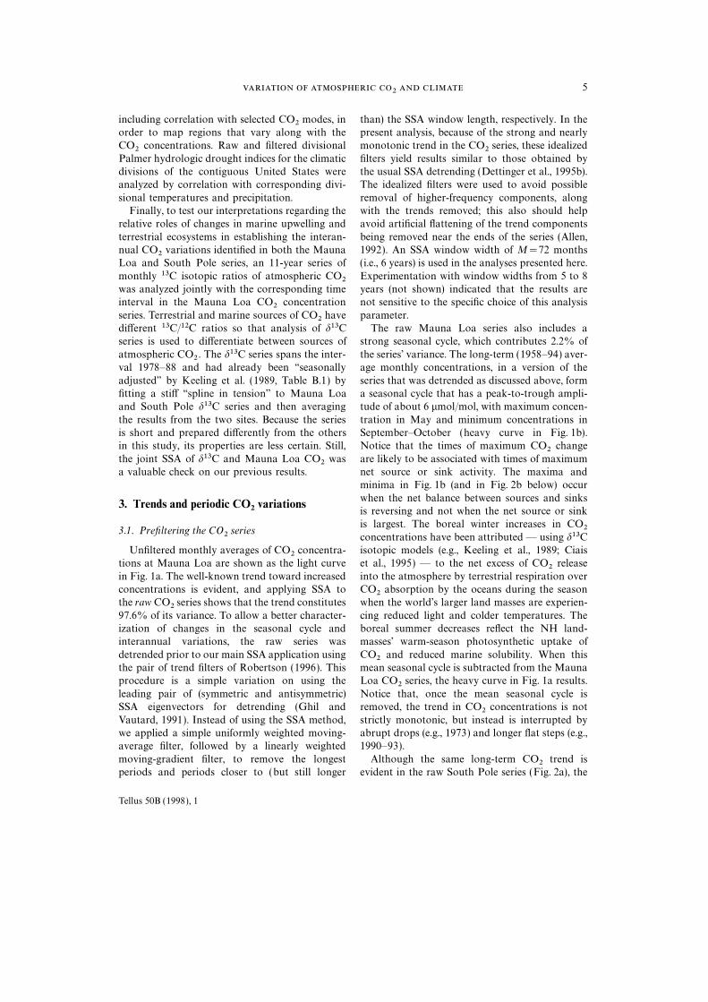
strong seasonal cycle, which contributes 2.2% ofseries is used to differentiate between sources of

atmospheric CO2 . The d13C series spans the inter- the series’ variance. The long-term (1958–94) aver-age monthly concentrations, in a version of theval 1978–88 and had already been ‘‘seasonally

adjusted’’ by Keeling et al. (1989, Table B.1) by series that was detrended as discussed above, forma seasonal cycle that has a peak-to-trough ampli-fitting a stiff ‘‘spline in tension’’ to Mauna Loa

and South Pole d13C series and then averaging tude of about 6 mmol/mol, with maximum concen-

tration in May and minimum concentrations inthe results from the two sites. Because the seriesis short and prepared differently from the others September–October (heavy curve in Fig. 1b).

Notice that the times of maximum CO2 changein this study, its properties are less certain. Still,

the joint SSA of d13C and Mauna Loa CO2 was are likely to be associated with times of maximumnet source or sink activity. The maxima anda valuable check on our previous results.minima in Fig. 1b (and in Fig. 2b below) occur

when the net balance between sources and sinks3. Trends and periodic CO

2variations

is reversing and not when the net source or sinkis largest. The boreal winter increases in CO23.1. Prefiltering the CO

2series

concentrations have been attributed — using d13Cisotopic models (e.g., Keeling et al., 1989; CiaisUnfiltered monthly averages of CO2 concentra-

tions at Mauna Loa are shown as the light curve et al., 1995) — to the net excess of CO2 release

into the atmosphere by terrestrial respiration overin Fig. 1a. The well-known trend toward increasedconcentrations is evident, and applying SSA to CO2 absorption by the oceans during the season

when the world’s larger land masses are experien-the raw CO2 series shows that the trend constitutes

97.6% of its variance. To allow a better character- cing reduced light and colder temperatures. Theboreal summer decreases reflect the NH land-ization of changes in the seasonal cycle and

interannual variations, the raw series was masses’ warm-season photosynthetic uptake of

CO2 and reduced marine solubility. When thisdetrended prior to our main SSA application usingthe pair of trend filters of Robertson (1996). This mean seasonal cycle is subtracted from the Mauna

Loa CO2 series, the heavy curve in Fig. 1a results.procedure is a simple variation on using the

leading pair of (symmetric and antisymmetric) Notice that, once the mean seasonal cycle isremoved, the trend in CO2 concentrations is notSSA eigenvectors for detrending (Ghil and

Vautard, 1991). Instead of using the SSA method, strictly monotonic, but instead is interrupted byabrupt drops (e.g., 1973) and longer flat steps (e.g.,we applied a simple uniformly weighted moving-

average filter, followed by a linearly weighted 1990–93).

Although the same long-term CO2 trend ismoving-gradient filter, to remove the longestperiods and periods closer to (but still longer evident in the raw South Pole series (Fig. 2a), the

Tellus 50B (1998), 1

. . . 6

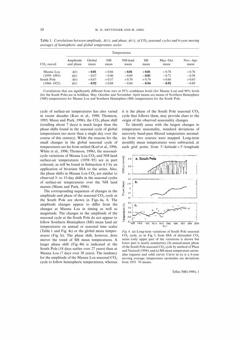
Fig. 1. Variations in CO2 concentrations (mmol/mol) at Mauna Loa, Hawaii, as (a) unfiltered mean-monthly concen-trations ( light solid) and concentrations with monthly-mean seasonal cycle subtracted (heavy solid); (b) monthly-mean seasonal CO2 cycle (January–December) from all years of record of detrended CO2 series (solid), as well asfrom first part (dotted), and last part (dashed) of record; and (c) detrended CO2 concentrations with monthly-meanseasonal cycle for the entire record removed. Solid arrowheads in panel (b) indicate months in which the 1958–72and 1980–94 means are significantly different from each other, according to a Student-t test, with confidence levelsgreater than 95%. Monthly-mean seasonal cycles are computed from monthly means after the series was detrendedby Robertson’s (1996) method.

Tellus 50B (1998), 1

2 7

Fig. 2. Same as Fig. 1, except for variations of CO2 concentrations at the South Pole. Raw data in Fig. 2a are difficultto discern from the deseasonalized series. Arrowheads in panel (b) indicate months in which differences between1965–77 and 1981–93 means are significantly different from each other at the 90% confidence level.

Tellus 50B (1998), 1

. . . 8

seasonal cycle is much smaller than at Mauna tion of detrending. Although the shift is difficultto discern in these monthly data, mean MarchLoa. The seasonal CO2 cycle at the South Pole is

so small that the raw series ( light curve) in Fig. 2a and mean September concentrations seem to have

increased and decreased, respectively, so as tois lost in the thick ‘‘deseasonalized’’ curve. Thelong-term mean seasonal cycle at the South Pole hasten the arrival of the spring maximum and

autumn minimum of CO2 . Thus, along with an(Fig. 2b) is out of phase with the Mauna Loa

cycle, reflecting Southern Hemisphere seasons. increase in amplitude, the phase of the seasonalCO2 cycle has shifted towards earlier in the yearAlthough not shown here, CO2 records from Point

Barrow in northern Alaska (Keeling and Whorf, in recent decades. Similar shifts towards an earlier

seasonal cycle are more obvious at the South Pole1994) and Alert Station near northwest Greenland(Conway et al., 1994) also have seasonal cycles (Fig. 2b) where the shift is imposed on a smaller

overall cycle and at Point Barrow (not shown)that are very different from those at Mauna Loa

or the South Pole; the Arctic seasonal cycles are where it is imposed on a very asymmetric cycle.The detrended Mauna Loa series retains a largemuch larger than at Mauna Loa and also are

shaped differently, with an asymmetric form dom- seasonal cycle that limits the interpretation of the

faint interannual signals. The analysis of interan-inated by a brief, deep CO2minimum in Septemberand October that reflects the brief surge of photo- nual variations was based, therefore, on a

detrended and deseasonalized version of the CO2synthesis during the short Arctic summers (Ciais

et al., 1995). Thus, seasonal CO2 cycles vary series (Figs. 1c, 2c). These series were obtained bydetrending the ‘‘deseasonalized’’ heavy curves insignificantly from place to place in response to

local uptake and release of CO2 at the surface of Figs. 1a, 2a. Significant subannual, seasonal, andinterannual variability remain in these series,land and oceans.

The seasonal CO2 cycles at both Mauna Loa although the magnitude of these variations is but

a small fraction of the raw CO2 variability.and the South Pole have changed with time. Forexample, it is apparent in Fig. 1a that removal ofthe long-term average seasonal cycle does not

3.2. L ong-term variations of the seasonal CO2cycle

remove all the seasonal variations from the MaunaLoa series. Notice that the heavy, deseasonalized The depiction of the changing seasonal cycles

using the series in Figs. 1c and 2c is complicatedcurve in Fig. 1a shows little seasonal variation in

the early years of the record, but, by the 1990s, by a resulting characterization of smaller-than-average seasonal cycles during the time intervalhas clear annual residuals that are in phase with

the mean seasonal cycle and almost one-third as centered on the 1970s as having negative ampli-

tudes. To simplify visualization, therefore, we per-large as it. Thus, the seasonal cycle of CO2 concen-trations, as noted already by Bacastow et al. formed a separate SSA on detrended but not

deseasonalized CO2 series (which does not yield(1985), has increased in recent decades well

beyond its long-term average amplitude. negative amplitudes) for the discussions in thissection, whereas in the remainder of this paper,The 15-year-mean seasonal cycles from the

beginning and end of a detrended version of the CO2 variations will be discussed in terms of the

SSA of the detrended and deseasonalized seriesMauna Loa CO2 series are shown as dotted anddashed curves in Fig. 1b. Comparison of the three (Figs. 1c, 2c).

Variations of the seasonal CO2 cycle’s amplitudecurves in Fig. 1b indicates that the average change

in the seasonal CO2 cycle, from the beginning to were characterized by SSA of the detrended butnot deseasonalized CO2 series, with a windowthe end of the Mauna Loa record, occurred mainly

as an increase by +1 mmol/mol in the cycle’s width of 72 months. The SSA results for the

detrended Mauna Loa series are dominated bypeak-to-trough range. The nearly symmetrictiming of the largest changes, positive and nega- the mean seasonal cycle and its long-term vari-

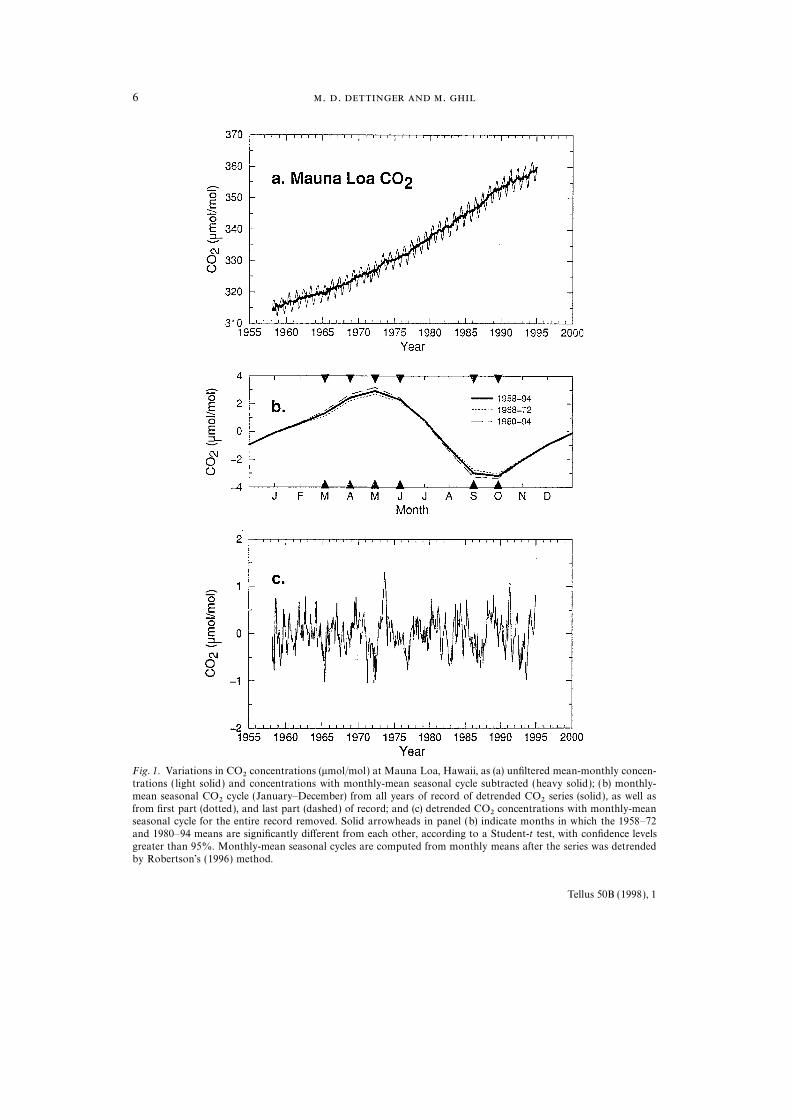
ations. The boreal-winter variations are illustratedtive, in Fig. 1b is largely an artifact of the detrend-ing, so it is difficult to decide during which seasons in Fig. 3a; the envelope of boreal-summer vari-

ations (not shown) is virtually the negative of theCO2 has increased or decreased most, except in

relative terms. The shape of the seasonal cycle has envelope shown. The time-varying amplitude(heavy curve, Fig. 3a) and changes in phasechanged slightly, however, and this is not a func-

Tellus 50B (1998), 1

2 9

parallels the progression of global and NH meantemperatures in recent decades (Fig. 3c).Correlations of the amplitudes and phases of the

Mauna Loa (and South Pole) seasonal CO2 cycleswith long-term global and hemispheric surface-airtemperature trends are listed in Table 1. Variations

of the amplitude of the seasonal CO2 cycle atMauna Loa correlate well with global-mean tem-peratures and NH-land temperatures, but less well

with overall NH-mean temperatures. The ampli-tude of the seasonal CO2 cycle is about equallycorrelated with NH summer and winter temper-

atures, but the correlation coefficient for thosetwo temperature series is also 0.90 (giving a con-fidence level greater than 95%).

The parallel between global temperatures andthe amplitude of the seasonal cycle of CO2 concen-trations has been noted by Keeling et al. (1996),Fig. 3. (a) Long-term variations of Mauna Loa seasonal

CO2 cycle, from singular-spectrum analysis (SSA) of using other time-series analysis methods based ondetrended CO2 series, as sum of reconstructed SSA com- fitted harmonics and splines in tension (Keelingponents 1 and 2 (light curve) and amplitude envelope by et al., 1989). They have suggested that the recentmethod of Plaut and Vautard (1994) (heavy curve); (b)

warmer climate has fostered vegetation growthannual-mean phase of Mauna Loa seasonal CO2 cycle

and attendant increases in photosynthesis, andby method of Plaut and Vautard (1994); and (c) Northerndecreases in CO2 , during the warm seasons andHemisphere (NH) mean temperature anomalies (squares

and solid curve) and global-mean temperature anomalies increased respiration, with increases in CO2 ,(triangles and dashed curve). Only the positive upper during the cool nongrowing seasons. Nemry et al.part of the variations is shown in (a) but the negative (1996) used a mechanistic vegetation model topart is essentially symmetric. Curves in (c) are 6-year

show that, in most of the NH, temperate eco-moving averages; temperature anomalies are deviations

systems dominate the seasonal CO2 cycle but,from the 1951–70 means.near the latitude of Mauna Loa (21°N), tropicalecosystems could dominate. For the slow vari-ations of seasonality shown in Fig. 3, the various(Fig. 3b) of the seasonal CO2 cycle were deter-

mined by annually averaging the direction and hemispheric temperatures all share much the sametrend and the source of seasonal-cycle changesamplitude, in the complex plane, of a complex-

valued time series with real part equal to the SSA can not be distinguished by correlations alone.

The CO2 seasonality trends also are broadly sim-reconstruction (light curve, Fig. 3a) and imaginarypart equal to its time rate of change (see Plaut ilar to recent global land-precipitation trends

(Keeling et al., 1995), although Knorr andand Vautard, 1994, and Moron et al., in press, for

other uses of this decomposition). The Mauna Heimann (1995) argue that water availability haslittle impact on the seasonal CO2 cycle. DespiteLoa seasonal CO2 cycle is characterized by rela-

tively stable amplitudes in the 1960s, a decrease these uncertainties, SSA provides a particularly

clear picture of the history of the CO2 variationsto minimum amplitudes around 1970, a rapidincrease through the 1970s, another slight min- for use in more detailed interpretations.

The changing phase of the seasonal CO2 cycleimum around 1987, and then renewed increases

until at least 1994. The phase of the seasonal CO2 at Mauna Loa may be associated with changingtemperature seasons over the NH land masses.cycle has shifted towards progressively earlier

occurrence of the seasons, totalling about 8 days Table 1 indicates that the changing phase of theseasonal CO2 cycle at Mauna Loa is only modestlybetween 1958 and 1995, with local maxima in

1968 and 1981. correlated with the global and hemispheric tem-

perature trends (given the few degrees of freedomThe sequence of changes in the amplitude ofthe seasonal CO2 cycle at Mauna Loa nearly in these smoothed series). Although the seasonal

Tellus 50B (1998), 1

. . . 10

Table 1. Correlations between amplitude, A(t), and phase, w(t), of CO2seasonal cycles and 6-year moving

averages of hemispheric and global temperature series

Temperatures

Amplitude Global NH NH-land SH May–Oct. Nov.–Apr.CO2 record and phase mean mean mean mean mean mean

Mauna Loa A(t) +0.81 +0.66 +0.81 +0.81 +0.78 +0.76(1959–1993) w(t) −0.67 −0.46 −0.69 −0.81 −0.71 −0.58

South Pole A(t) +0.67 +0.57 +0.70 +0.74 +0.66 +0.65(1966–1922) w(t) −0.92 +0.88 −0.84 −0.94 −0.92 −0.89

Correlations that are significantly different from zero at 95% confidence levels (for Mauna Loa) and 90% levels(for the South Pole) are in boldface. May–October and November–April means are means of Northern Hemisphere(NH) temperatures for Mauna Loa and Southern Hemisphere (SH) temperatures for the South Pole.

cycle of surface-air temperatures has also varied it is the phase of the South Pole seasonal CO2cycle that follows them, may provide clues to thein recent decades (Kuo et al., 1990; Thomson,

1995; Mann and Park, 1996), the CO2 phase shift origin of the observed seasonality changes.To identify areas with the largest changes in(totalling about 7 days) is much larger than the

phase shifts found in the seasonal cycle of global temperature seasonality, standard deviations ofnarrowly band-pass filtered temperature anomal-temperatures (no more than a single day over the

course of this century). While the reasons for the ies from two sources were mapped. Long-term

monthly mean temperatures were subtracted, atsmall changes in the global seasonal cycle oftemperatures are far from settled (Karl et al., 1996; each grid point, from 5°-latitude×5°-longitudeWhite et al., 1996; Thomson, 1996), the seasonal-

cycle variations of Mauna Loa CO2 and NH-landsurface-air temperatures (1958–95) are in partcoherent, as will be found in Subsection 4.3 by an

application of bivariate SSA to the series. Also,the phase shifts in Mauna Loa CO2 are similar toobserved 5- to 15-day shifts in the seasonal cycles

of surface-air temperatures over the NH landmasses (Mann and Park, 1996).

The corresponding sequences of changes in the

amplitude and phase of the seasonal CO2 cycle atthe South Pole are shown in Figs. 4a, b. Theamplitude changes appear to differ from the

changes at Mauna Loa in timing as well asmagnitude. The changes in the amplitude of theseasonal cycle at the South Pole do not appear to

follow Southern Hemisphere (SH) mean land airtemperatures on annual or seasonal time scales(Table 1 and Fig. 4c) or the global mean temper- Fig. 4. (a) Long-term variations of South Pole seasonal

CO2 cycle, as in Fig. 3, from SSA of detrended CO2atures (Fig. 3c). The phase shift, however, doesseries (only upper part of the variations is shown butmirror the trend of SH mean temperatures. Alower part is nearly symmetric); (b) annual-mean phaselarger phase shift (Fig. 4b) is indicated at theof the South Pole seasonal CO2 cycle by method of Plaut

South Pole (18 days earlier over 27 years) than atand Vautard (1994); and (c) SH mean temperature anom-

Mauna Loa (7 days over 38 years). The tendency alies (squares and solid curve). Curve in (c) is a 6-yearfor the amplitude of the Mauna Loa seasonal CO2 moving average; temperature anomalies are deviations

from 1951–70 means.cycle to follow hemispheric temperatures, whereas

Tellus 50B (1998), 1

2 11

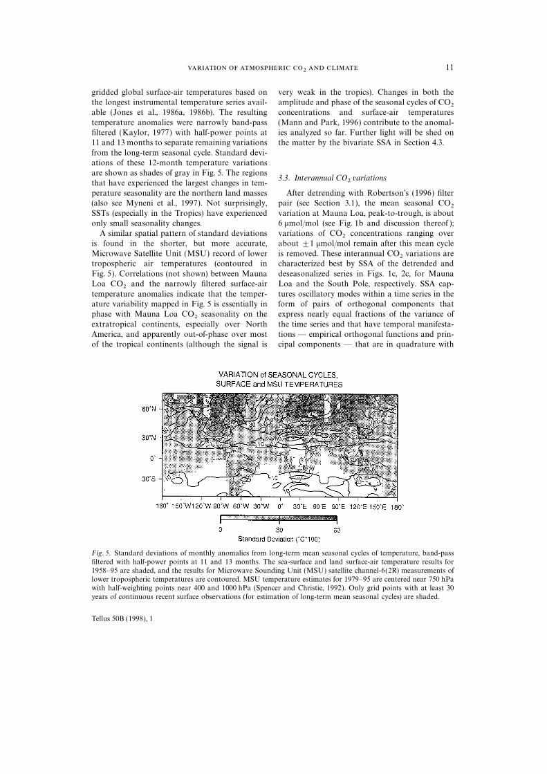
gridded global surface-air temperatures based on very weak in the tropics). Changes in both theamplitude and phase of the seasonal cycles of CO2the longest instrumental temperature series avail-

able (Jones et al., 1986a, 1986b). The resulting concentrations and surface-air temperatures

(Mann and Park, 1996) contribute to the anomal-temperature anomalies were narrowly band-passfiltered (Kaylor, 1977) with half-power points at ies analyzed so far. Further light will be shed on

the matter by the bivariate SSA in Section 4.3.11 and 13 months to separate remaining variations

from the long-term seasonal cycle. Standard devi-ations of these 12-month temperature variationsare shown as shades of gray in Fig. 5. The regions

3.3. Interannual CO2variations

that have experienced the largest changes in tem-perature seasonality are the northern land masses After detrending with Robertson’s (1996) filter

pair (see Section 3.1), the mean seasonal CO2(also see Myneni et al., 1997). Not surprisingly,

SSTs (especially in the Tropics) have experienced variation at Mauna Loa, peak-to-trough, is about6 mmol/mol (see Fig. 1b and discussion thereof );only small seasonality changes.

A similar spatial pattern of standard deviations variations of CO2 concentrations ranging over

about ±1 mmol/mol remain after this mean cycleis found in the shorter, but more accurate,Microwave Satellite Unit (MSU) record of lower is removed. These interannual CO2 variations are

characterized best by SSA of the detrended andtropospheric air temperatures (contoured in

Fig. 5). Correlations (not shown) between Mauna deseasonalized series in Figs. 1c, 2c, for MaunaLoa and the South Pole, respectively. SSA cap-Loa CO2 and the narrowly filtered surface-air

temperature anomalies indicate that the temper- tures oscillatory modes within a time series in theform of pairs of orthogonal components thatature variability mapped in Fig. 5 is essentially in

phase with Mauna Loa CO2 seasonality on the express nearly equal fractions of the variance of

the time series and that have temporal manifesta-extratropical continents, especially over NorthAmerica, and apparently out-of-phase over most tions — empirical orthogonal functions and prin-

cipal components — that are in quadrature withof the tropical continents (although the signal is

Fig. 5. Standard deviations of monthly anomalies from long-term mean seasonal cycles of temperature, band-passfiltered with half-power points at 11 and 13 months. The sea-surface and land surface-air temperature results for1958–95 are shaded, and the results for Microwave Sounding Unit (MSU) satellite channel-6(2R) measurements oflower tropospheric temperatures are contoured. MSU temperature estimates for 1979–95 are centered near 750 hPawith half-weighting points near 400 and 1000 hPa (Spencer and Christie, 1992). Only grid points with at least 30years of continuous recent surface observations (for estimation of long-term mean seasonal cycles) are shaded.

Tellus 50B (1998), 1

. . . 12

each other (Vautard and Ghil, 1989; Dettingeret al., 1995b).

In the present SSAs, we address CO2 variations

that are probably not reflections of simple dynam-ical oscillations but rather reflect many concurrentprocesses. Thus, in analyzing these variations, our

focus is on the characterization of concentrated,but broad-peak, variance rather than single, puresine waves. In this analysis, therefore, significance

tests that compare SSA components to ideal sinewaves (Allen and Smith, 1996) are probably notsuitable. Instead, we used simple considerations

to focus analysis on the most powerful compon-ents. Later, these components are shown to berelated to SST oscillations with frequencies like

tropical-temperature modes that have been foundto be highly significant relative to the most rigor-ous statistical tests (Allen and Smith, 1996; Mann

and Park, 1996).Using the same 72-month window as before,

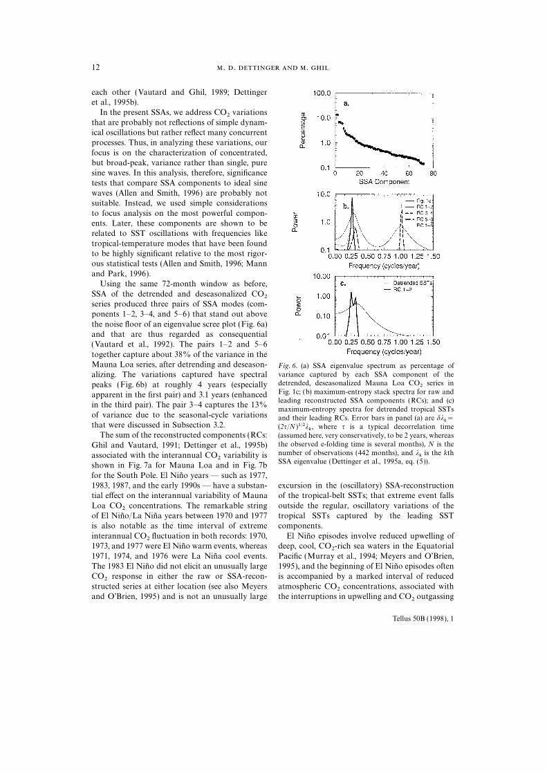
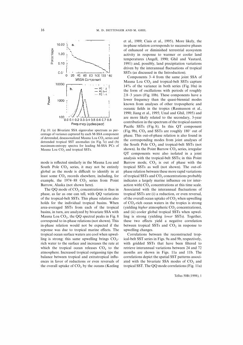
SSA of the detrended and deseasonalized CO2series produced three pairs of SSA modes (com-ponents 1–2, 3–4, and 5–6) that stand out above

the noise floor of an eigenvalue scree plot (Fig. 6a)and that are thus regarded as consequential(Vautard et al., 1992). The pairs 1–2 and 5–6

together capture about 38% of the variance in theMauna Loa series, after detrending and deseason- Fig. 6. (a) SSA eigenvalue spectrum as percentage of

variance captured by each SSA component of thealizing. The variations captured have spectraldetrended, deseasonalized Mauna Loa CO2 series inpeaks (Fig. 6b) at roughly 4 years (especiallyFig. 1c; (b) maximum-entropy stack spectra for raw andapparent in the first pair) and 3.1 years (enhancedleading reconstructed SSA components (RCs); and (c)

in the third pair). The pair 3–4 captures the 13%maximum-entropy spectra for detrended tropical SSTs

of variance due to the seasonal-cycle variations and their leading RCs. Error bars in panel (a) are dlk=

that were discussed in Subsection 3.2. (2t/N)1/2lk, where t is a typical decorrelation time

The sum of the reconstructed components (RCs: (assumed here, very conservatively, to be 2 years, whereasthe observed e-folding time is several months), N is theGhil and Vautard, 1991; Dettinger et al., 1995b)number of observations (442 months), and l

kis the kthassociated with the interannual CO2 variability is

SSA eigenvalue (Dettinger et al., 1995a, eq. (5)).shown in Fig. 7a for Mauna Loa and in Fig. 7b

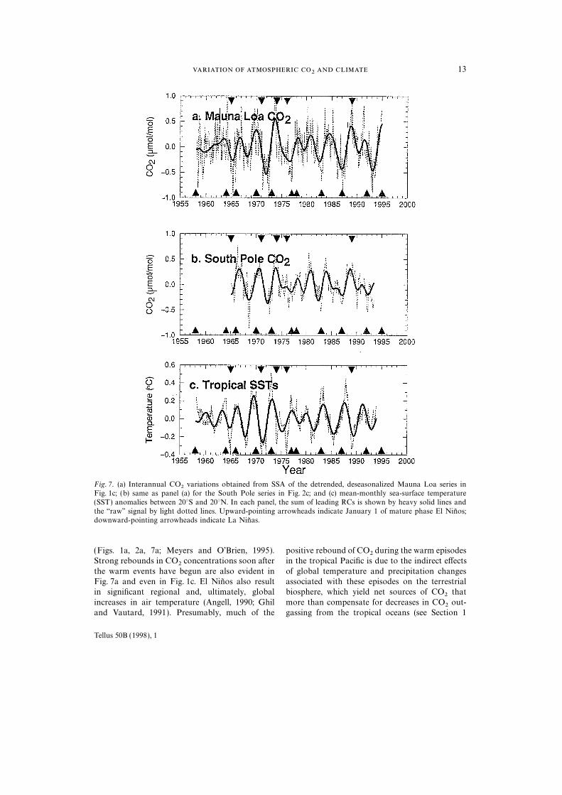
for the South Pole. El Nino years — such as 1977,1983, 1987, and the early 1990s — have a substan- excursion in the (oscillatory) SSA-reconstruction

of the tropical-belt SSTs; that extreme event fallstial effect on the interannual variability of Mauna

Loa CO2 concentrations. The remarkable string outside the regular, oscillatory variations of thetropical SSTs captured by the leading SSTof El Nino/La Nina years between 1970 and 1977

is also notable as the time interval of extreme components.

El Nino episodes involve reduced upwelling ofinterannual CO2 fluctuation in both records: 1970,1973, and 1977 were El Nino warm events, whereas deep, cool, CO2-rich sea waters in the Equatorial

Pacific (Murray et al., 1994; Meyers and O’Brien,1971, 1974, and 1976 were La Nina cool events.The 1983 El Nino did not elicit an unusually large 1995), and the beginning of El Nino episodes often

is accompanied by a marked interval of reducedCO2 response in either the raw or SSA-recon-

structed series at either location (see also Meyers atmospheric CO2 concentrations, associated withthe interruptions in upwelling and CO2 outgassingand O’Brien, 1995) and is not an unusually large

Tellus 50B (1998), 1

2 13

Fig. 7. (a) Interannual CO2 variations obtained from SSA of the detrended, deseasonalized Mauna Loa series inFig. 1c; (b) same as panel (a) for the South Pole series in Fig. 2c; and (c) mean-monthly sea-surface temperature(SST) anomalies between 20°S and 20°N. In each panel, the sum of leading RCs is shown by heavy solid lines andthe ‘‘raw’’ signal by light dotted lines. Upward-pointing arrowheads indicate January 1 of mature phase El Ninos;downward-pointing arrowheads indicate La Ninas.

(Figs. 1a, 2a, 7a; Meyers and O’Brien, 1995). positive rebound of CO2 during the warm episodesin the tropical Pacific is due to the indirect effectsStrong rebounds in CO2 concentrations soon after

the warm events have begun are also evident in of global temperature and precipitation changesassociated with these episodes on the terrestrialFig. 7a and even in Fig. 1c. El Ninos also result

in significant regional and, ultimately, global biosphere, which yield net sources of CO2 that

more than compensate for decreases in CO2 out-increases in air temperature (Angell, 1990; Ghiland Vautard, 1991). Presumably, much of the gassing from the tropical oceans (see Section 1

Tellus 50B (1998), 1

. . . 14

and Keeling et al., 1989; Siegenthaler, 1990). LaNinas followed by El Ninos in rapid successioncontribute some of the appearance of CO2 declines

at the beginning of El Ninos. Finally, both theinitial CO2 decline and the eventual resurgencemay reflect the overall lag between SST and CO2variations (discussed in greater detail later). TheMauna Loa interannual variations in Fig. 7a areshared with the South Pole CO2 series, as indi-

cated by the close correspondence between theinterannual components extracted from the twoseries by separate univariate SSA (Fig. 7b) as well

as by a bivariate SSA of the two series (not shown).Interannual variations of the mean SSTs in the

global tropics between 20°S and 20°N (isolated

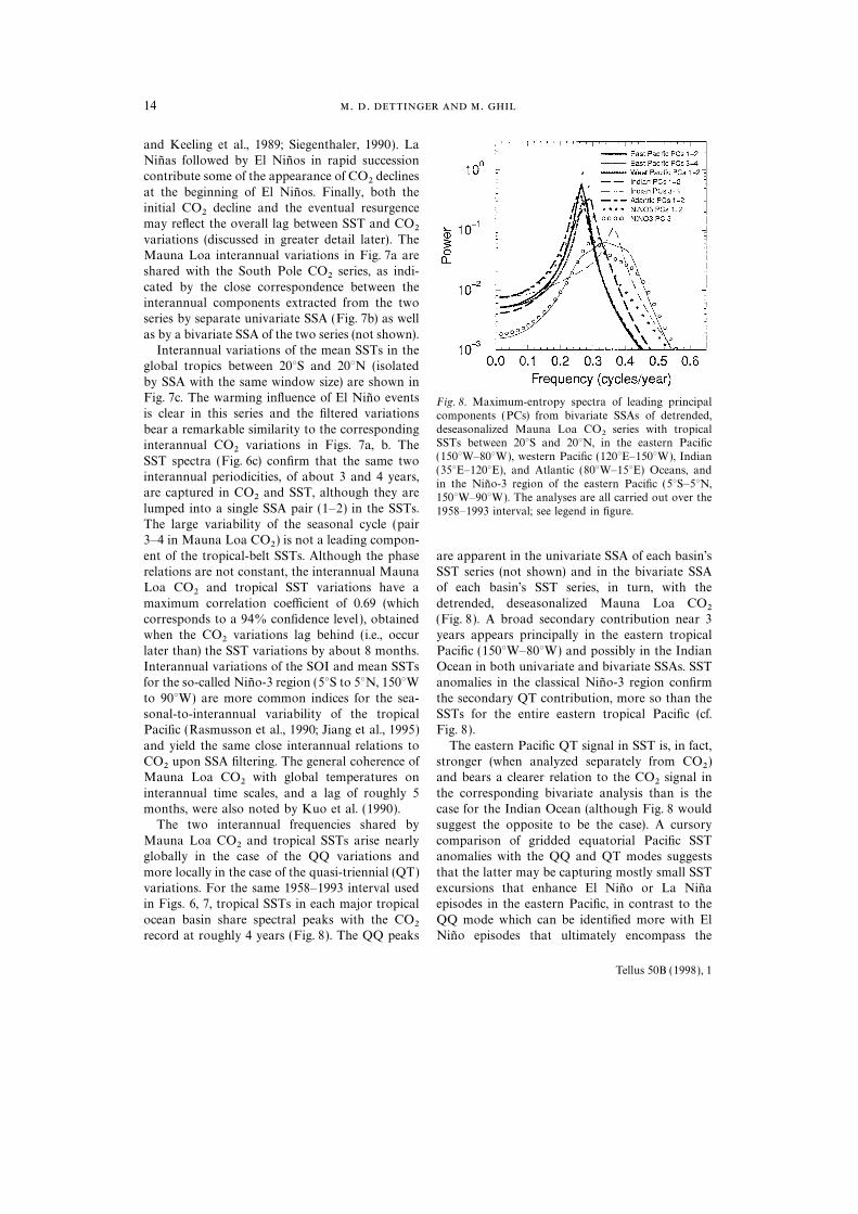
by SSA with the same window size) are shown inFig. 7c. The warming influence of El Nino events Fig. 8. Maximum-entropy spectra of leading principalis clear in this series and the filtered variations components (PCs) from bivariate SSAs of detrended,

deseasonalized Mauna Loa CO2 series with tropicalbear a remarkable similarity to the correspondingSSTs between 20°S and 20°N, in the eastern Pacificinterannual CO2 variations in Figs. 7a, b. The(150°W–80°W), western Pacific (120°E–150°W), IndianSST spectra (Fig. 6c) confirm that the same two(35°E–120°E), and Atlantic (80°W–15°E) Oceans, and

interannual periodicities, of about 3 and 4 years,in the Nino-3 region of the eastern Pacific (5°S–5°N,

are captured in CO2 and SST, although they are 150°W–90°W). The analyses are all carried out over thelumped into a single SSA pair (1–2) in the SSTs. 1958–1993 interval; see legend in figure.The large variability of the seasonal cycle (pair3–4 in Mauna Loa CO2 ) is not a leading compon-

ent of the tropical-belt SSTs. Although the phase are apparent in the univariate SSA of each basin’sSST series (not shown) and in the bivariate SSArelations are not constant, the interannual Mauna

Loa CO2 and tropical SST variations have a of each basin’s SST series, in turn, with the

detrended, deseasonalized Mauna Loa CO2maximum correlation coefficient of 0.69 (whichcorresponds to a 94% confidence level ), obtained (Fig. 8). A broad secondary contribution near 3

years appears principally in the eastern tropicalwhen the CO2 variations lag behind (i.e., occur

later than) the SST variations by about 8 months. Pacific (150°W–80°W) and possibly in the IndianOcean in both univariate and bivariate SSAs. SSTInterannual variations of the SOI and mean SSTs

for the so-called Nino-3 region (5°S to 5°N, 150°W anomalies in the classical Nino-3 region confirm

the secondary QT contribution, more so than theto 90°W) are more common indices for the sea-sonal-to-interannual variability of the tropical SSTs for the entire eastern tropical Pacific (cf.

Fig. 8).Pacific (Rasmusson et al., 1990; Jiang et al., 1995)

and yield the same close interannual relations to The eastern Pacific QT signal in SST is, in fact,stronger (when analyzed separately from CO2 )CO2 upon SSA filtering. The general coherence of

Mauna Loa CO2 with global temperatures on and bears a clearer relation to the CO2 signal in

the corresponding bivariate analysis than is theinterannual time scales, and a lag of roughly 5months, were also noted by Kuo et al. (1990). case for the Indian Ocean (although Fig. 8 would

suggest the opposite to be the case). A cursoryThe two interannual frequencies shared by

Mauna Loa CO2 and tropical SSTs arise nearly comparison of gridded equatorial Pacific SSTanomalies with the QQ and QT modes suggestsglobally in the case of the QQ variations and

more locally in the case of the quasi-triennial (QT) that the latter may be capturing mostly small SSTexcursions that enhance El Nino or La Ninavariations. For the same 1958–1993 interval used

in Figs. 6, 7, tropical SSTs in each major tropical episodes in the eastern Pacific, in contrast to the

QQ mode which can be identified more with Elocean basin share spectral peaks with the CO2record at roughly 4 years (Fig. 8). The QQ peaks Nino episodes that ultimately encompass the

Tellus 50B (1998), 1

2 15

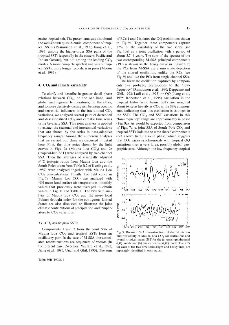
entire tropical belt. The present analysis also found of RCs 1 and 2 isolates the QQ oscillations shownin Fig. 9a. Together these components capturethe well-known quasi-biennial component of trop-

ical SSTs (Rasmusson et al., 1990; Jiang et al., 27% of the variability of the two series (see

Fig. 10a) as a joint oscillation with a period of1995) among the higher-order SSA pairs of thetropical SSTs (especially in the eastern Pacific and about 3.7–4 years. The sum of the spectra of the

two corresponding M-SSA principal componentsIndian Oceans), but not among the leading CO2modes. A more complete spectral analysis of trop- (PC) is shown as the heavy curve in Figure 10b;

the PCs from M-SSA are a univariate depictionical SSTs, using longer records, is in press (Moronet al., 1997). of the shared oscillation, unlike the RCs (see

Fig. 9) and like the PCs from single-channel SSA.The bivariate oscillation captured by compon-

ents 1–2 probably corresponds to the ‘‘low-4. CO2and climate variability

frequency’’ (Rasmusson et al., 1990; Keppenne andGhil, 1992; Latif et al., 1993) or QQ (Jiang et al.,To clarify and describe in greater detail phase

relations between CO2 , on the one hand, and 1995; Robertson et al., 1995) oscillation in the

tropical Indo-Pacific basin. SSTs are weightedglobal and regional temperatures, on the other,and to more decisively distinguish between oceanic about twice as heavily as CO2 in the SSA compon-

ents, indicating that this oscillation is stronger inand terrestrial influences in the interannual CO2variations, we analyzed several pairs of detrended the SSTs. The CO2 and SST variations in this

‘‘low-frequency’’ range are approximately in phaseand deseasonalized CO2 and climatic time series

using bivariate SSA. This joint analysis is applied (Fig. 9a). As would be expected from comparisonof Figs. 7a–c, joint SSA of South Pole CO2 andto extract the seasonal and interannual variations

that are shared by the series in data-adaptive tropical SSTs isolates the same shared components

(not shown here), also in phase, which suggestsfrequency ranges. Among the numerous analysesthat we carried out, three are discussed in detail that CO2 varies synchronously with tropical QQ

variations over a very large, possibly global geo-here. First, the time series shown by the light

curves in Figs. 7a (Mauna Loa CO2 ) and 7c graphic area. Although the low-frequency tropical(tropical-belt SST) were analyzed by two-channelSSA. Then the averages of seasonally adjusted

d13C isotopic ratios from Mauna Loa and theSouth Pole (taken from Table B.2 of Keeling et al.,1989) were analyzed together with Mauna Loa

CO2 concentrations. Finally, the light curve inFig. 7a (Mauna Loa CO2 ) was analyzed withNH-mean land surface-air temperatures (monthly

values that previously were averaged to obtainvalues in Fig. 3c and Table 1). The bivariate ana-lysis of Mauna Loa CO2 and the more local

Palmer drought index for the contiguous UnitedStates are also discussed, to illustrate the jointclimatic contributions of precipitation and temper-

ature to CO2 variations.

4.1. CO2and tropical SST s

Components 1 and 2 from the joint SSA ofFig. 9. Bivariate SSA reconstructions of shared interan-Mauna Loa CO2 and tropical SSTs form annual variability of Mauna Loa CO2 concentrations and

oscillatory pair. In the case of M-SSA, the associ-overall tropical-mean, SST for the (a) quasi-quadrennial

ated reconstructions are sequences of vectors (in (QQ) mode and (b) quasi-triennial (QT) mode. The RCsthe present case, 2-vectors: Vautard et al., 1992; for each of the two time series ( light and heavy lines) are

separately identified in each panel.Jiang et al., 1995; Unal and Ghil, 1995). The sum

Tellus 50B (1998), 1

. . . 16

et al., 1989; Ciais et al., 1995). More likely, thein-phase relation corresponds to successive phasesof enhanced or diminished terrestrial ecosystem

activity in response to warmer or cooler landtemperatures (Angell, 1990; Ghil and Vautard,1991) and, possibly, land precipitation variations

driven by the interannual fluctuations of tropicalSSTs (as discussed in the Introduction).

Components 3–4 from the same joint SSA of

Mauna Loa CO2 and tropical-belt SSTs capture14% of the variance in both series (Fig. 10a) inthe form of oscillations with periods of roughly

2.8–3 years (Fig. 10b). These components have alower frequency than the quasi-biennial modesknown from analyses of other tropospheric and

oceanic fields in the tropics (Rasmusson et al.,1990; Jiang et al., 1995; Unal and Ghil, 1995) andare more likely related to the secondary, 3-year

contribution in the spectrum of the tropical easternPacific SSTs (Fig. 8). In this QT component

Fig. 10. (a) Bivariate SSA eigenvalue spectrum as per- (Fig. 9b), CO2 and SSTs are roughly 180° out ofcentage of variance captured by each M-SSA component phase. This out-of-phase relation is also found inof detrended, deseasonalized Mauna Loa CO2 series and

the corresponding modes from joint analyses ofdetrended tropical SST anomalies (in Fig. 7c) and (b)

the South Pole CO2 and tropical-belt SSTs (notmaximum-entropy spectra for leading M-SSA PCs ofshown). In the Point Barrow CO2 series, irregularMauna Loa CO2 and tropical SSTs.QT components were also isolated in a joint

analysis with the tropical-belt SSTs; in this PointBarrow mode, CO2 is out of phase with themode is reflected similarly in the Mauna Loa and

South Pole CO2 series, it may not be entirely tropical SSTs as well (not shown). The out-of-

phase relation between these more rapid variationsglobal as the mode is difficult to identify in atleast some CO2 records elsewhere, including, for of tropical SSTs and CO2 concentrations probably

indicates a largely marine influence on (or inter-example, the 1974–88 CO2 series from Point

Barrow, Alaska (not shown here). action with) CO2 concentrations at this time scale.Associated with the interannual fluctuations ofThe QQ mode of CO2 concentrations is thus in

phase, as far as one can tell, with QQ variations tropical SSTs are (i) a reduction, or even reversal,

of the overall ocean uptake of CO2 when upwellingof the tropical-belt SSTs. This phase relation alsoholds for the individual tropical basins. When of CO2-rich ocean waters in the tropics is strong

(yielding higher atmospheric CO2 concentrations),area-averaged SSTs from each of the tropical

basins, in turn, are analyzed by bivariate SSA with and (ii) cooler global tropical SSTs when upwel-ling is strong (yielding lower SSTs). Together,Mauna Loa CO2 , the QQ spectral peaks in Fig. 8

correspond to in-phase relations (not shown). This these two effects yield a negative correlation

between tropical SSTs and CO2 in response toin-phase relation would not be expected if thereponse was due to tropical marine effects. The upwelling changes.

Correlations between the reconstructed trop-tropical ocean surface waters are cool when upwel-

ling is strong; this same upwelling brings CO2- ical-belt SST series in Figs. 9a and 9b, respectively,with gridded SSTs that have been filtered torich water to the surface and increases the rate at

which the tropical ocean releases CO2 to the retrieve interannual variations between 24 and 72months are shown in Figs. 11a and 11b. Theatmosphere. Increased tropical outgassing tips the

balance between tropical and extratropical influ- correlations depict the spatial SST patterns associ-

ated with the bivariate SSA modes of CO2 andences in favor of reductions or even reversals ofthe overall uptake of CO2 by the oceans (Keeling tropical SST. The QQ mode correlations (Fig. 11a)

Tellus 50B (1998), 1

2 17

Fig. 11. Correlations between tropical-belt SST modes shared with Mauna Loa CO2 (Fig. 9), on the one hand, andgridded global SSTs, band-pass filtered with half-power points at 24 and 72 months, on the other; (a) QQ mode(Fig. 9a) and (b) QT mode (Fig. 9b). Contours depict (dimensionless) correlations times 100, where significantlydifferent from zero at the 90% confidence level; dashed where negative.

are strong over most of the Pacific and Indian Pacific, near the Nino-3 region used routinely tomonitor El Nino conditions.Oceans and the tropical Atlantic, with positive

correlations throughout most of the tropics. Taken together, the QQ and QT components

reproduce much of the (variably) lagged relationRecalling that the SST in the QQ bivariate SSAmode is in phase with Mauna Loa CO2 , the between SST and CO2 noted in the interannual

components isolated from independent (univari-strong, widespread positive correlations in Fig. 11a

indicate that near global SST warming underlies ate) SSAs of Mauna Loa CO2 and tropical-beltSSTs (Figs. 7a, c, respectively). Summing the RCthe positive QQ variations in CO2 . In contrast,

the QT mode correlations (Fig. 11b) are strong curves of CO2 , on the one hand, and the SST

curves, on the other, yields a maximum cross-almost exclusively in the tropical and subtropicaleastern Pacific; elsewhere, the correlations are correlation between the interannual variabilities

(QQ and QT) of CO2 and SST that equals +0.65much weaker. Recall that the QT mode had CO2and tropical SST out of phase; therefore, Fig. 11b (i.e., provides a 92% confidence level) when the

lag equals 6 months, with SST on average leadingimplies that atmospheric QT-scale CO2 increases

accompany mostly decreases in SST (and presum- CO2 . This is quite close to the correlation of+0.69 (statistical significance of 94%) at 8 monthsably increased upwelling) in the eastern tropical

Tellus 50B (1998), 1

. . . 18

lag when the two series were filtered throughseparate univariate SSAs. As importantly, the vari-ations in lags of the univariate RCs and bivariate

RCs are similar over most of the 38 years of CO2record (except near the beginning and end whereSSA reconstructions are least constrained).

4.2. CO2concentrations and d13C isotopic ratios

Fig. 12. Bivariate SSA reconstruction of the leadingTo better understand the contrast between the (QQ) mode of shared interannual variability of Mauna

in-phase QQ relation of tropical SSTs and CO2 Loa CO2 and the average of seasonally adjusted d13Cseries from Mauna Loa and the South Pole.versus the out-of-phase QT relation, the detrended

and deseasonalized Mauna Loa CO2 concentra-tion series and a ‘‘seasonally adjusted’’ global d13C among the leading SSA components: remaining

components (not shown) are primarily in the 1–2.5series for atmospheric CO2 were analyzed together

using bivariate SSA. The d13C of CO2 in the year range, with some lower frequency contamina-tion. No significant seasonal variation survived inatmosphere and oceans equilibrate with each other

rapidly so that they are almost always near iso- the ‘‘seasonally adjusted’’ d13C, although a CO2seasonal component was isolated by the jointtopic equilibrium on the time scales of interest

here; as a consequence, at a given time, CO2 that analysis (not shown).

The out-of-phase QQ relation between CO2enters the atmosphere from the oceans has almostthe same isotopic signature as the CO2 that is and d13C is consistent with a terrestrial origin for

the QQ variations in CO2 because terrestrialalready in the atmosphere. In contrast, d13C in

CO2 from terrestrial sources (including fossil fuels) sources of CO2 will tend to depress the d13C evenas they contribute to elevated CO2 concentrations.is typically about −18 per mil lower (lower

13C/12C ratio) than the oceanic and atmospheric In contrast, the QT CO2 mode is not present

among the shared CO2 and d13C variationsreservoirs (Keeling et al., 1989). Using this differ-ence, measured variations of d13C in the atmo- because this CO2 mode is dominated by the

influence of upwelling variations in the easternsphere have been used to isolate relative

contributions of marine and terrestrial CO2 Pacific ‘‘source’’ area on atmospheric CO2 , whichdoes not directly modify atmospheric d13C.sources (Keeling et al., 1989; Ciais et al., 1995). In

the present study, the joint analysis of CO2 and

d13C series thus provides a direct line of evidence4.3. CO

2and NH continental climate

for understanding the differences between QQ andQT variations in CO2 concentrations. Interannual d13C variations thus indicate

differing CO2 sources for the QQ and QT modes,The ‘‘global’’ d13C series used in the bivariateSSA with Mauna Loa CO2 was obtained by with the QQ mode likely to have mostly terrestrial

origins. To investigate these QQ origins further,averaging the seasonally adjusted d13C at Mauna

Loa and the South Pole (averaging performed by various NH and continental climate series werecompared, using joint SSA, to the Mauna LoaKeeling et al., 1989, table B.2). A shared QQ mode

was isolated by using a window length of 50 CO2 series. Results were mixed, however, because

continental series tended to exhibit a somewhatmonths (to accommodate the short length of thed13C record); this mode captures 29% of variance different mix of frequencies than either the Mauna

Loa CO2 or tropical SST series.(Fig. 12). No distinct QT variation was found

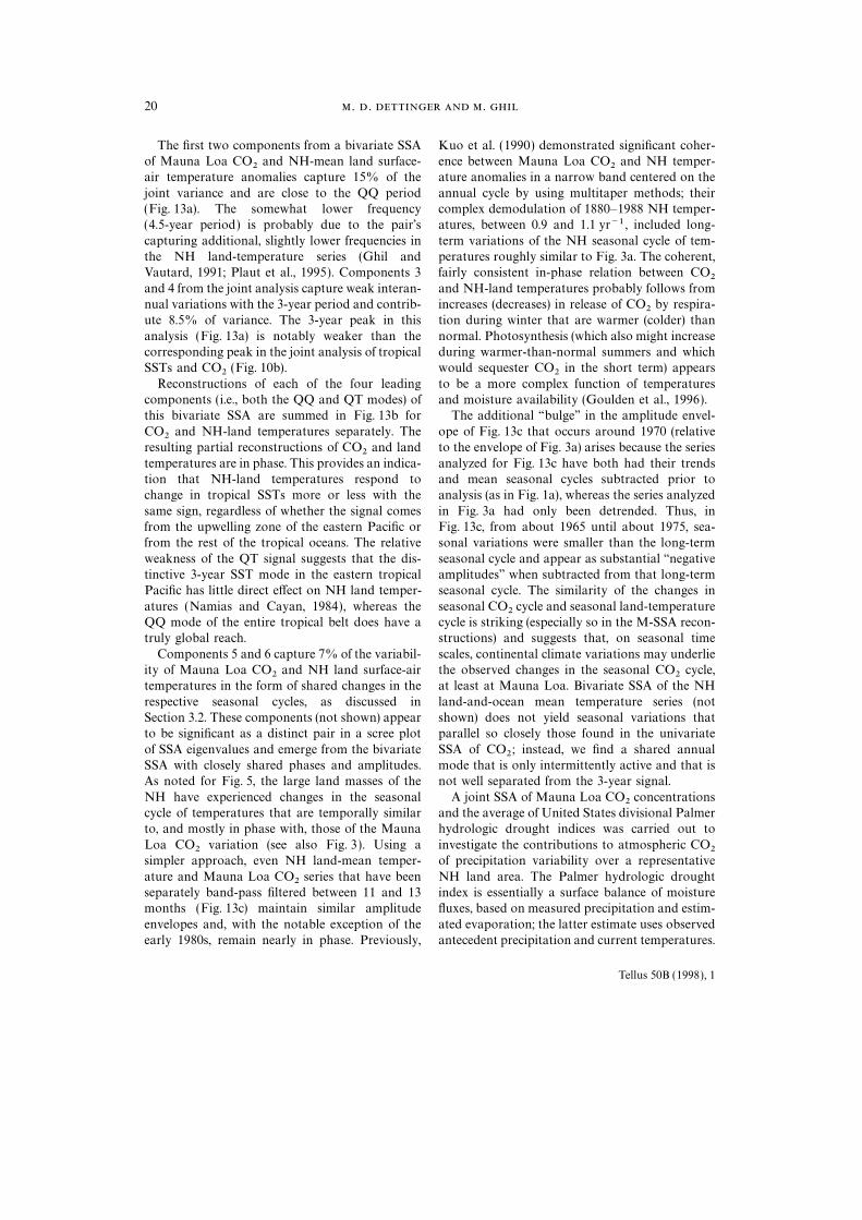
Fig. 13. (a) Maximum-entropy spectrum of leading PCs from bivariate SSA detrended, deseasonalized Mauna LoaCO2 series (Fig. 1c) and NH mean land surface-air temperature anomalies (Fig. 3c). (b) Reconstructions of leadingcomponents from the bivariate SSA of CO2 and NH land temperatures for interannual (QQ and QT) time scales.(c) CO2 and NH land-temperature anomalies, separately band-pass filtered (Kaylor, 1977) with half-power pointsat 11 and 13 months. (d) Reconstruction of leading components from bivariate SSA of Mauna Loa CO2 and thearea-weighted average of Palmer hydrologic drought indices for United States climate divisions.

Tellus 50B (1998), 1

2 19

Fig. 13.

Tellus 50B (1998), 1

. . . 20

The first two components from a bivariate SSA Kuo et al. (1990) demonstrated significant coher-ence between Mauna Loa CO2 and NH temper-of Mauna Loa CO2 and NH-mean land surface-

air temperature anomalies capture 15% of the ature anomalies in a narrow band centered on the

annual cycle by using multitaper methods; theirjoint variance and are close to the QQ period(Fig. 13a). The somewhat lower frequency complex demodulation of 1880–1988 NH temper-

atures, between 0.9 and 1.1 yr−1 , included long-(4.5-year period) is probably due to the pair’s

capturing additional, slightly lower frequencies in term variations of the NH seasonal cycle of tem-peratures roughly similar to Fig. 3a. The coherent,the NH land-temperature series (Ghil and

Vautard, 1991; Plaut et al., 1995). Components 3 fairly consistent in-phase relation between CO2and NH-land temperatures probably follows fromand 4 from the joint analysis capture weak interan-

nual variations with the 3-year period and contrib- increases (decreases) in release of CO2 by respira-tion during winter that are warmer (colder) thanute 8.5% of variance. The 3-year peak in this

analysis (Fig. 13a) is notably weaker than the normal. Photosynthesis (which also might increaseduring warmer-than-normal summers and whichcorresponding peak in the joint analysis of tropical

SSTs and CO2 (Fig. 10b). would sequester CO2 in the short term) appears

to be a more complex function of temperaturesReconstructions of each of the four leadingcomponents (i.e., both the QQ and QT modes) of and moisture availability (Goulden et al., 1996).

The additional ‘‘bulge’’ in the amplitude envel-this bivariate SSA are summed in Fig. 13b for

CO2 and NH-land temperatures separately. The ope of Fig. 13c that occurs around 1970 (relativeto the envelope of Fig. 3a) arises because the seriesresulting partial reconstructions of CO2 and land

temperatures are in phase. This provides an indica- analyzed for Fig. 13c have both had their trendsand mean seasonal cycles subtracted prior totion that NH-land temperatures respond to

change in tropical SSTs more or less with the analysis (as in Fig. 1a), whereas the series analyzed

in Fig. 3a had only been detrended. Thus, insame sign, regardless of whether the signal comesfrom the upwelling zone of the eastern Pacific or Fig. 13c, from about 1965 until about 1975, sea-

sonal variations were smaller than the long-termfrom the rest of the tropical oceans. The relative

weakness of the QT signal suggests that the dis- seasonal cycle and appear as substantial ‘‘negativeamplitudes’’ when subtracted from that long-termtinctive 3-year SST mode in the eastern tropical

Pacific has little direct effect on NH land temper- seasonal cycle. The similarity of the changes in

seasonal CO2 cycle and seasonal land-temperatureatures (Namias and Cayan, 1984), whereas theQQ mode of the entire tropical belt does have a cycle is striking (especially so in the M-SSA recon-

structions) and suggests that, on seasonal timetruly global reach.

Components 5 and 6 capture 7% of the variabil- scales, continental climate variations may underliethe observed changes in the seasonal CO2 cycle,ity of Mauna Loa CO2 and NH land surface-air

temperatures in the form of shared changes in the at least at Mauna Loa. Bivariate SSA of the NH

land-and-ocean mean temperature series (notrespective seasonal cycles, as discussed inSection 3.2. These components (not shown) appear shown) does not yield seasonal variations that

parallel so closely those found in the univariateto be significant as a distinct pair in a scree plot

of SSA eigenvalues and emerge from the bivariate SSA of CO2 ; instead, we find a shared annualmode that is only intermittently active and that isSSA with closely shared phases and amplitudes.

As noted for Fig. 5, the large land masses of the not well separated from the 3-year signal.

A joint SSA of Mauna Loa CO2 concentrationsNH have experienced changes in the seasonalcycle of temperatures that are temporally similar and the average of United States divisional Palmer

hydrologic drought indices was carried out toto, and mostly in phase with, those of the Mauna

Loa CO2 variation (see also Fig. 3). Using a investigate the contributions to atmospheric CO2of precipitation variability over a representativesimpler approach, even NH land-mean temper-

ature and Mauna Loa CO2 series that have been NH land area. The Palmer hydrologic droughtindex is essentially a surface balance of moistureseparately band-pass filtered between 11 and 13

months (Fig. 13c) maintain similar amplitude fluxes, based on measured precipitation and estim-

ated evaporation; the latter estimate uses observedenvelopes and, with the notable exception of theearly 1980s, remain nearly in phase. Previously, antecedent precipitation and current temperatures.

Tellus 50B (1998), 1

2 21

When the drought index is positive, wet soil- South Pole that appear to be consonant withtropical processes (Fig. 7). These interannual vari-moisture conditions predominate and terrestrial

ecosystems are expected to flourish; when it is ations can be further decomposed into two modes,

quasi-quadrennial (QQ) and quasi-triennial (QT).negative, dry conditions prevail.QQ-like variations of CO2 and Palmer drought The QQ mode isolated by using joint SSA of CO2

and tropical SSTs has CO2 variations that areindices, but not QT variations, emerged from the

joint analysis. The leading four components com- stronger and in phase with the corresponding SSTs(Fig. 9a). The QQ modes are associated with globalprise a mix of frequencies, with dominant periods

of 3.6–4.1 years. The sum of these four components temperature variations (Figs. 8 and 11a) and their

CO2 expression is probably a response to terrestrial(Fig. 13d) does not display a consistent phaserelation between CO2 and the drought index, each ecosystem changes associated with temperature

variations on global scales. In particular, as temper-of which can lead or lag the other. This variable

phasing of CO2 and drought indices may reflect atures increase, respiration increases in terrestrialecosystems and the balance between the CO2the complexity of the time lags and interactions

between precipitation and temperature anomalies sources and sinks is shifted temporarily towards the

sources (see Section 1). If the temperature increasesthat form the indices. Although soil-moisture con-ditions presumably play an important role in CO2 are large enough and widespread enough, regional

and global CO2 concentrations increase.variability, that role apparently is not as simple

and amenable to isolation by a linear analysis Bivariate SSAs of CO2 and various tropicalclimate indices (including tropical-belt sea-surfacesuch as SSA as are the temperature-CO2 relations.

No notable variation of the seasonal cycle was temperatures (SSTs)) also isolates a shared QTmode in which CO2 and SST participation arefound in the drought index series.180° out-of-phase (Fig. 9b). This mode appears to

derive from the roughly 3-year fluctuations of SSTin the eastern Tropical Pacific (Figs. 8 and 11b).5. Summary and conclusionsA simple explanation for this out-of-phase relation

might be that anomalously weak upwelling ofThe present study has used univariate singular-spectrum analysis (SSA) to isolate seasonal and cool, CO2-rich ocean water in the eastern tropical

Pacific reduces CO2 outgassing there, decreasesinterannual variations of atmospheric CO2 concen-

trations at Mauna Loa Observatory and the South atmospheric CO2 , and increases tropical SSTduring El Nino events; the opposite occurs duringPole (Figs. 1, 2); bivariate SSA analyses were used

to relate these variations to various climate indices, La Nina episodes. These changes in tropical ocean

upwelling are evidently large enough to be feltglobal and regional. The univariate analyses illus-trate long-term changes in the amplitude of the nearly globally in CO2 levels, whereas the SST

and climate effects are much more regional.seasonal CO2 cycle that are regional in nature and

that, at least at Mauna Loa, follow the low-frequency Joint SSA of Mauna Loa CO2 with a seasonallyadjusted atmospheric d13C series yields strong QQcourse of hemispheric mean air temperatures

(Fig. 3), as well as the changes in temperature components that are out of phase with each other

(Fig. 12). No variations with a distinct 3-yearseasonality over Northern Hemisphere (NH) landmasses (Figs. 5, 13c). Changes in the phase of the period were found. These amplitudes and phase

relations support the hypothesis that QT vari-seasonal CO2 cycle at the South Pole are larger

than those at Mauna Loa and mirror hemispheric ations of CO2 at Mauna Loa and the South Poleare dominated by marine influences on atmo-and global temperature trends (Fig. 4). Recent

changes in the seasonal cycle of CO2 variation at spheric CO2 concentrations, presumably following

the relatively localized upwelling variations in theboth locations include a hastening of the onset ofwinter and summer CO2 sources and sinks, for each eastern tropical Pacific. Although upwelling vari-

ations undoubtedly contribute to the QQ vari-hemisphere separately (Figs. 1b, 2b), and a generalincrease in amplitude of the seasonal CO2 cycle in ations in CO2 , the latter are dominated by the

effects of the near-global QQ temperature vari-both locations.

Univariate SSA also isolates interannual CO2 ations on terrestrial climate, ecosystems responseand, through them, CO2 concentrations.variations at both Mauna Loa (Fig. 6) and the

Tellus 50B (1998), 1

. . . 22

Joint SSA of Mauna Loa CO2 with NH-land surface-air temperatures, and North Americandrought indices. Marine-upwelling variabilitymean air temperature anomalies isolated shared

variations with annual, QQ, and much weaker appears to directly influence the QT mode of

atmospheric CO2 concentrations and is presum-QT periods. CO2 and continental NH temperaturevariations appear to be generally in phase in all ably present also in the QQ mode. The QQ

climate mode, however, involves temperature andthree narrow frequency bands considered (Figs.

13b, c). The interannual variations in continental precipitation variations over much broader areasthat include the large NH land masses. Thetemperature seasonality shared with Mauna Loa

CO2 are similar and in phase, to a remarkable responses of terrestrial ecosystems to these farflung

QQ climate variations dominate over QQ upwel-extent (Fig. 13c). The results of bivariate SSA alsosuggest a northern continental source for the CO2 ling effects in the interannual CO2 variations at

both Mauna Loa and the South Pole.seasonality changes.

Analysis of Palmer drought indices — as surrog-ates for soil moisture and hence ecosystem vigor —in the United States revealed only QQ-like modes 6. Acknowledgementsin common with CO2 . Presumably, the climaticeffects of the QQ tropical and global ocean climate This work benefited greatly from access to the

U. S. Department of Energy’s (DOE’s) Carbonmode on North American climate and ecosystems

are considerably stronger than the effects of the Dioxide Information Analysis Center’s variousdata archives, from climatic time series providedmore localized QT, eastern tropical Pacific mode.

The QQ drought-index variations shared with by D. R. Cayan at the Scripps Institution ofOceanography (SIO) and J. Eischeid of NOAA’sCO2 do not exhibit a consistent phase relation

between the two time series. Indeed, correlations Climate Data Center, and from isotopic time series

provided by P. Tans and M. Trolier of NOAA’sbetween temperatures, precipitation, tropical cli-mate indices, and drought indices across the Climate Monitoring and Diagnostics Laboratory.

Our ongoing interactions with the SSA GroupUnited States (not shown) revealed a complex

interleaving of regional temperature and precipita- and Toolkit makers greatly facilitated our analysisof all these time series. Comments from and discus-tion influences that determine the drought indices

for specific seasons on interannual time scales. sions with D. R. Cayan, with V. Moron from the

Universite de Bourgogne, Dijon, and withTo summarize, univariate and bivariate SSAhas helped isolate and reconstruct annual, QT, C. Penland, M. Hoerling, and Klaus Weickmann

of the NOAA Climate Diagnostics Center contrib-and QQ modes of CO2 variability at Mauna Loa

and the South Pole. The interannual CO2 vari- uted also. E. Bainto at SIO’s Climate ResearchDivision provided graphical support. MD’s workations are strongly linked with variations of trop-

ical SSTs: ocean upwelling in the eastern tropical was supported by the U. S. Geological Survey’s

Global Change Hydrology Program. MG’sPacific dominates the QT mode, and global cli-mate and biosphere responses to tropical-belt SST research was supported at UCLA by NSF grant

ATM95–23787, and at the Ecole Normalevariations dominate the QQ mode. A substantial

effect of NH terrestrial climate on CO2 concentra- Superieure by a Elf-Aquitaine/CNRS Chair of theAcademie des Sciences, Paris. This is publicationtions has also been identified by the bivariate SSA

and by simple correlation analyses with atmo- no. 4893 of UCLA’s Institute of Geophysics and

Planetary Physics.spheric 13C/12C isotopic ratios, continental NH

REFERENCES

Allen, M. R. 1992. Interactions between the atmosphere perature after adjustment for the El Nino influence,1958–89. Geophys. Res. L ett. 17, 1093–1096.and oceans on time scales of weeks to years. PhD thesis,

St. John’s College, Oxford, 203 p. Bacastow, R. B., Keeling, C. D. and Whorf, T. P. 1985.Seasonal amplitude increase in atmospheric CO2 con-Allen, M. R., and Smith, L. A. 1996. Monte Carlo SSA:

Detecting irregular oscillations in the presence of col- centration at Mauna Loa, Hawaii, 1959–82. J. Geo-phys. Res. 90, 10 529–10 540.ored noise. J. Clim. 9, 3373–3404.

Angell, J. K. 1990. Variation in global tropospheric tem- Broomhead, D. S. and King, G. 1986. Extracting qualit-

Tellus 50B (1998), 1

2 23

ative dynamics from experimental data. Physica D ations: 1851–1984. J. Climate Appl. Meteorol. 25,1213–1230.20, 217–236.

Jones, P. D., Wigley, T. M. L. and Wright, P. B. 1986c.Chang, P., Wang, B. and Link, J. 1994. InteractionsGlobal temperature variations between 1861 and 1984.between the seasonal cycle and the Southern Oscilla-Nature 322, 430–434.tion–Frequency entrainment and chaos in a coupled

Karl, T. R., Jones, P. D. and Knight, R. W. 1996. Testingocean-atmosphere model. Geophys. Res. L ett. 21,for bias in the climate record. Science 271, 1879–1880.2817–2820.

Kaylor, R. E. 1977. Filtering and decimation of digitalCiais, P., Tans, P. P., Trolier, M., White, J. W. C. andtime series. Univ. of Maryland, Dept. of MeterologyFrancey, R. J. 1995. A large Northern HemisphereTech. Note BN850 (Engineering and Physical Sciencesterrestrial CO2 sink indicated by 13C/12C ratio ofLibrary, Univ. of Maryland), 14 p.atmospheric CO2 . Science 269, 1098–1102.

Keeling, C. D. and Whorf, T. P. 1994. Atmospheric CO2Colebrook, J. M. 1978. Continuous plankton records–records from sites in the SIO air sampling network.Zooplankton and environment, northeast Atlantic andIn: T rends ‘93: A compendium of data on global changeNorth Sea, 1948–1975. Oceanol. Acta 1, 9–23.(eds. T. A. Boden, Kaiser, D. P., Sepanski, R. J. andConway, T. J., Tans, P. P., Waterman, L. S., Thoning,Stoss, F. W.). ORNL/CDIAC-65. Carbon DioxideK. W., Kitzis, D. R., Masarie, K. A. and Zhang, N.Information Analysis Center, Oak Ridge National1994. Evidence for interannual variability of theLaboratory, Oak Ridge, Tenn., pp. 16–26.carbon cycle from the National Oceanic and Atmo-

Keeling, C. D., Bacastow, R. B., Bainbridge, A. E.,spheric Administration/Climate Monitoring and Dia-Ekdahl, C. E., Jr., Guenther, P. R., Waterman, L. S.gnostics Laboratory global air sampling network.and Chin, J. F. S. 1976. Atmospheric carbon dioxideJ. Geophys. Res. 99, 22831–22855.variations at Mauna Loa observatory, Hawaii. T ellusDettinger, M. D., Ghil, M. and Keppenne, C. L. 1995a.28, 538–551.Interannual and interdecadal variability of United

Keeling, C. D., Bacastow, R. B. and Whorf, T. P. 1982.States surface-air temperatures, 1910–1987. ClimaticMeasurements of the concentrations of carbon dioxideChange 31, 35–66.at Mauna Loa observatory, Hawaii. In: Carbon dioxideDettinger, M. D., Ghil, M., Strong, C. M., Weibel, W.review: 1982 (ed. C. Clark). Oxford University Press,

and Yiou, P. 1995b. Software expedites singular-New York, 377–385.

spectrum analysis of noisy time series. Eos, T rans.Keeling, C. D., Bacastow, R. B., Carter, A. F., Piper,

AGU 76, 12, 14, 21.S. C., Whorf, T. P., Heimann, M., Mook, W. G. and

Fraedrich, K. 1986. Estimating the dimensions of weatherRoeloffzen, H. 1989. A three-dimensional model of

and climate attractors. J. Atmos. Sci. 43, 419–432.atmospheric CO2 transport based on observed winds:

Francey, R. J., Tans, P. P., Allison, C. E., Enting, I. G.,1. Analysis of observational data. In: Aspects of climate

White, J. W. C. and Trolier, M. 1995. Changes invariability in the Pacific and the Western Americas (ed.

oceanic and terrestrial carbon uptake since 1982.D. H. Peterson). AGU Geophysical Monograph 55,

Nature 373, 326–330.165–236.

Ghil, M. and Vautard, R. 1991. Interdecadal oscillations Keeling, C. D., Chin, J. F. S. and Whorf, T. P. 1996.and the warming trend in global temperature time Increased activity of northern vegetation inferred fromseries. Nature 350, 324–327. atmospheric CO2 measurements. Nature 382, 146–149.

Ghil, M. and Yiou, P. 1996. Spectral methods: What Keeling, C. D., Whorf, T. P., Wahlen, M. and van derthey can and cannot do for climatic time series. In: Plicht, J. 1995. Interannual extremes in the rate of riseDecadal climate variability: Dynamics and predictability of atmospheric carbon dioxide since 1980. Nature(D. Anderson Willebrand, eds.). Elsevier, pp. 445–482 375, 666–670.

Goulden, M. L., Munger, J. W., Fan, S. M., Daube, B. C., Keppenne, C. L. and Ghil, M. 1992. Adaptive spectraland Wofsy, S. C. 1996. Exchange of carbon dioxide by analysis and prediction of the Southern Oscillationa deciduous forest: Response to interannual climate Index. J. Geophys. Res. 97, 20 449–20 554.variability. Science 271, 1576–1578. Knorr, W. and Heimann, M. 1995. Impact of drought

Jiang, N., Neelin, D. and Ghil, M. 1995. Quasi- stress and other factors on seasonal land biospherequadrennial and quasi-biennial variability in the CO2 exchange studied through an atmospheric tracerequatorial Pacific. Clim. Dyn. 12, 101–112. transport model. T ellus 47B, 471–489.

Jin, F. F., Neelin, J. D. and Ghil, M. 1994. El Nino on Kuo, C., Lindberg, C. and Thomson, D. J. 1990. Coher-the Devil’s staircase: Annual subharmonic steps to ence established between atmospheric carbon dioxidechaos. Science 264, 70–72. and global temperature. Nature 343, 709–714.

Jones, P. D., Raper, S. C. B., Bradley, R. S., Diaz, H. F., Lambert, G., Monfray, P., Ardouin, B., Bonsang, G.,Kelly, P. M. and Wigley, T. M. L. 1986a. Northern Gaudry, A., Kazan, V. and Polian, G. 1995. Year-to-Hemisphere surface air temperature variations: year changes in atmospheric CO2 . T ellus 47B, 53–55.1851–1984. J. Climate Appl. Meteorol. 25, 161–79. Latif, M., Sterl, A., Maier-Reimer, E. and Junge, M. M.

Jones, P. D., Raper, S. C. B. and Wigley, T. M. L. 1986b. 1993. Structure and predictability of the El Nino/Southern Oscillation phenomenon in a coupled ocean-Southern Hemisphere surface air temperature vari-

Tellus 50B (1998), 1

. . . 24

atmosphere general circulation model. J. Clim. 6, North Pacific in a multi-century climate simulation.Clim. Dyn. 12, 227–242.700–708.

Mann, M. E. and Park, J. 1994. Global scale modes of Robertson, A. W., Ma, C. C., Ghil, M. and Mechoso,C. R. 1995. Simulation of the tropical Pacific climatesurface temperature variability on interannual to cen-

tury timescales. J. Geophys. Res. 99, 25 819–25 933. with a coupled ocean-atmosphere general circulationmodel. Part II: Interannual variability. J. Clim. 8,Mann, M. E. and Park, J. 1996. Greenhouse warming

and changes in the seasonal cycle of temperature: 1199–1216.Ropelewski, C. F. and Halpert, M. S. 1987. Global andModel versus observations. Geophys. Res. L ett. 23,

1111–1114. regional scale precipitation patterns associated withthe El Nino/Southern Oscillation. Monthly Wea. Rev.Meyers, S. D. and O’Brien, J. J. 1995. Pacific Ocean

influences atmospheric carbon dioxide. Eos, T rans. 115, 1606–1626.Sarmiento, J. L. 1993. Atmospheric CO2 stalled. NatureAGU 76, 533, 537.

Moron, V., Vautard, R. and Ghil, M. 1997. Trends, inter- 365, 697–698.Siegenthaler, U. 1990. El Nino and atmospheric CO2 .decadal and interannual oscillations in the global sea-

surface temperature. Clim. Dyn. in press. Nature 345, 295–296.Siegenthaler, U. and Sarmiento J. L. 1993. AtmosphericMurray, J. W., Barber, R. T., Roman, M. R., Bacon,

M. P., and Feely, R. A. 1994. Physical and biological carbon dioxide and the ocean. Nature 365, 119–125.Spencer, R. W. and Christie, J. R. 1992. Precision andcontrols on carbon cycling in the equatorial Pacific:

US JGOFS EqPac process study. Science 266, 58–65. radiosonde validation of satellite gridpoint temper-ature anomalies. Part II: A tropospheric retrieval andMyneni, R. B., Keeling, C. D. and Nemani, R. R. 1997.

Increased plant growth in the northern high latitudes trends during 1979–90. J. Clim. 5, 858–866.Suarez, M. J. and Schopf, P. S. 1988. A delayed actionfrom 1981 to 1991. Nature 386, 698–701.

Namias, J. and Cayan, D. R. 1984. El Nino: Implications oscillator for ENSO. J. Atmos. Sci. 45, 3283–3287.Sundquist, E. T. 1993. The global carbon dioxide budget.for forecasting. Oceanus 27, 41–47.

Nemry, B., Francois, L. Warnant, P. Roloinet F and Science 259, 934–941.Thomson, D. J. 1995. The seasons, global temperatures,Gerard, J.-C. 1996. The seasonality of the CO2

exchange between the atmosphere and the land bio- and precession. Science 268, 59–68.Thomson, D. J. 1996. Testing for bias in the climatesphere–A study with a global mechanistic vegetation

model. J. Geophys. Res. 101, 7111–7125. record. Science 271, 1881–1883.Trumbore, S. E., Chadwick, O. A. and Amundson, R.Okamoto, K., Tanimoto, S. and Okano, K. 1995. Statist-

ical analysis of the increase in atmospheric CO2 con- 1996. Rapid exchange between soil carbon and atmo-spheric carbon dioxide driven by temperature change.centrations and its relation to the possible existence

of CO2 fertilization on a global scale. T ellus 47B, Science 272, 393–396.Tziperman, E., Stone, L., Cane, M. A. and Jarosh, H.206–211.

Parker, D. E., Folland, C. K., Bevan, A., Ward, M. N., 1994. El Nino chaos: Overlapping of resonancesbetween the seasonal cycle and the Pacific ocean-Jackson, M., and Maskell, K. 1995. Marine surface

data for analysis of climatic fluctuations on interan- atmosphere oscillator. Science 264, 72–74.Unal, Y. S. and Ghil, M. 1995. Interannual and interdeca-nual to century timescales. In: Natural climate variabil-

ity on decade-to-century time scales (D. G. Martinson dal oscillation patterns in sea level. Clim. Dyn. 18,255–278.et al., eds.). National Academy Press, Washington, DC,

pp. 241–250. Vautard, R. and Ghil, M. 1989. Singular spectrum ana-lysis in nonlinear dynamics, with applications to paleo-Plaut, G. and Vautard, R. 1995. Spells of low-frequency

oscillations and weather regimes in the northern hemi- climatic time series. Physica D 35, 395–424.Vautard, R., Yiou, P. and Ghil, M. 1992. Singular-sphere. J. Atmos. Sciences 51, 210–236.

Press, W. H., Flannery, B. P., Teukolsky, S. A. and spectrum analysis: A toolkit for short, noisy chaoticsignals. Physica D 58, 95–126.Vetterling, W. T. 1989. Numerical recipes — the art of

scientific computing (FORTRAN Version). Cambridge White, O. R., Mende, W. and Beer, J. 1996. Testing forbias in the climate record. Science 271, 1880–1881.Univ. Press, New York, 702 pp.

Rasmusson, E. M., Wang, X. and Ropelewski, C. 1990. WMO 1984. Summary Report on the Status of the WMObackground air pollution monitoring network as at MayThe biennial component of ENSO variability. J. Mar.

Syst. 1, 71–96. 1984. World Meteorological Organization TechnicalDocument WMO/TD 13. Geneva, 21 pp.Robertson, A. W. 1996. Interdecadal variability over the

Tellus 50B (1998), 1