Seasonal Abundance, Age Structure, Gonadosomatic Index, and Gonad

Seasonal Abundance, Age Structure, Gonadosomatic Index, and Gonad

Histology of Yellow Bass Morone mississippiensis in the upper Barataria

Estuary, Louisiana

A Thesis

Submitted to the Graduate Faculty of

Nicholls State University

In partial fulfillment of the requirements for the degree of

Master of Science

in

Marine and Environmental Biology

by

Cynthia Nichole Fox

B.S., Tennessee Technological University, 2007

Spring 2010

i

CERTIFICATE

This is to certify that the thesis entitled “Seasonal Abundance, Age

Structure, Gonadosomatic Index, and Gonad Histology of Yellow Bass Morone

mississippiensis in the upper Barataria Estuary, Louisiana” submitted for the

award of Master of Science to Nicholls State University is a record of authentic,

original research conducted by Miss Cynthia Nichole Fox under our supervision

and guidance and that no part of this thesis has been submitted for the award of

any other degree, diploma, fellowship or other similar titles.

APPROVED: SIGNATURE: DATE:

Quenton Fontenot, Ph.D.

Assistant Professor of

Biological Sciences ____________________ _____________

Committee Chair

Allyse Ferrara, Ph.D.



Committee Member

Gary LaFleur, Jr., Ph.D.



Committee Member

ii

ABSTRACT

The Barataria Estuary is composed of interconnected lakes, bayous,

canals, cypress-tupelo swamps, hardwood forests and freshwater, intermediate,

brackish and salt marsh. The main riverine conduit source of the upper reaches of

the estuary is Bayou Chevreuil, which drains much of the area into Lac des

Allemands. Historically, the upper Barataria Estuary (UBE) received an annual

flood pulse from the Mississippi River until the construction of flood protection

levees. Since levee construction, water level in the upper estuary is a function of

precipitation. The lack of a natural annual flood pulse has altered the hydrology

of the upper Barataria Estuary.

The yellow bass Morone mississippiensis is a common, yet lesser known

species of the Mississippi River drainage basin. Yellow bass abundance in the

upper Barataria Estuary follows a seasonal migration pattern. The purpose of this

study was to gather basic life history data to better understand the ecological

niche of yellow bass in the Barataria Estuary, Louisiana. The goal of this study

was to assess a yellow bass population in the upper estuary by examining relative

seasonal abundance, age, gonadosomatic index (GSI), and gonad histology.

To quantify seasonal abundance, yellow bass were collected weekly to

biweekly from six sites in Lac des Allemands and Bayou Chevreuil using gill nets

from 14 November 2008 to 17 November 2009. Catch per unit effort (CPUE)

was calculated for each site for each date as a measure of relative abundance.

Mean CPUE values for each sample date were used to describe the relative

abundance of yellow bass in the upper Barataria Estuary. Dissolved oxygen

iii

(mg/L), salinity (ppt), temperature (°C), and specific conductance (µS) were

measured at each site and water level (m) and photoperiod (hrs) data were

obtained from USGS and US Naval Observatory, respectively, to determine if

environmental variables affected yellow bass abundance. CPUE was highest

from February-April, indicating yellow bass use the UBE seasonally. Yellow

bass abundance peaked as temperature reached approximately 18-22°C. Hypoxic

conditions (DO < 2.0 mg/L) were not recorded during this study; therefore it is

unknown how yellow bass abundance would be affected by low oxygen levels.

Total length (TL; mm), weight (WT; g), and GSI were measured for all

fish collected (N = 1,061). Age was estimated using saggital otoliths that were

sectioned with a low-speed saw (Buehler, St. Louis). Gonad samples (N = 200),

from fish collected throughout the year, were placed in 10% neutral buffered

formalin for histological analysis. Yellow bass age ranged from 1 to 4 years,

although no 3 year old fish were identified. The population was dominated by the

2 year old age class. GSI decreased as temperature reached 18-22°C, indicating

spawning had occurred. Spawning activity was confirmed histologically based on

the presence of post-ovulatory follicle complexes (POCs) in female gonads

collected from January 2009 to April 2009. As of May 2009, gonads of both

males and females, except for one female collected on 23 June 2009, were in the

“regressing” and “regenerating” stages and consisted of residual spermatozoa and

follicles, respectively, along with several early development stage spermatogonia

and oocytes.

iv

Results of this study indicate that yellow bass in the UBE mature by age 2

and spawn from early February through late April. The increase in yellow bass

abundance in early spring was directly related to spawning activity and not to

water quality or flood pulse.

v

ACKNOWLEDGEMENTS

First and foremost, I would like to express my sincere appreciation to my

advisor, Dr. Quenton Fontenot. The time, guidance, patience, and expertise that

he put into this project cannot be measured, and I am truly grateful. I would also

like to thank my committee members, Dr. Allyse Ferrara and Dr. Gary LaFleur,

Jr. for their help and support throughout my project.

I would like to thank Nicholls State University and the Bayousphere

Research Lab for the use of their vehicles, vessels, gear and funding for my

research. Thank you to all the graduate students who put in long days in the field

and long nights in the lab helping me collect and work up my fish. I could not

have done this without them. Special thanks go to Constance Kersten at McNeese

State University for processing my histology slides and Nancy Brown-Peterson at

Gulf Coast Research Laboratory for her vast knowledge and continuous help with

histology. Also, to Andy Fischer at Louisiana State University for his training and

assistance in the art of otolith aging.

Bob and Rama Smith provided me with a great deal of monetary support

during my project, and for that I will be eternally grateful. Thank you to Chris

Holt for reminding me at my lowest moments that everything would turn out

alright and be worth it.

Lastly, I want to express my deepest gratitude to my mother, Peggy Fox

and brother, Jason Fox. Thank you both so much for always supporting and

believing in me and for helping me make this dream come true.

vi

TABLE OF CONTENTS

Certificate ….………………………………………………………………………i

Abstract …………………………………………………………………………...ii

Acknowledgements …………………………………………………………….....v

Table of Contents ………………………………………………………………...vi

List of Figures …………………………………………………………………...vii

List of Tables ……………………………………………………………………..x

Introduction ……………………………………………………………………….1

Methods ………………………………………………………………………….13

Results …………………………………………………………………………...23

Discussion ……………………………………………………………………….56

Recommendations ……………………………………………………………….65

Literature Cited ………………………………………………………………….66

Appendix I ………………………………………………………………………74

Appendix II ……………………………………………………………………...78

Appendix III ……………………………………………………………………..83

Biographical Sketch ……………………………………………………………..90

Curriculum Vitae ………………………………………………………………..91

vii

LIST OF FIGURES

Figure 1. Distribution of yellow bass in the United States. The bold outline

delineates the Mississippi River drainage basin. ..……………………2

Figure 2. Female yellow bass (TL=263 mm) collected 23 January 2009 from the

upper Barataria Estuary, Louisiana (photograph by Cynthia Fox).

…………………………………………………………………………4

Figure 3. The Barataria Estuary (shaded region) in southeast Louisiana.

……........................................................................................................7

Figure 4. Major waterways (solid lines) and roadways (dashed lines) of the

upper Barataria Estuary, Louisiana. ..…………………………………9

Figure 5. Locations of the six study sites in Lac des Allemands (sites 1-3) and

Bayou Chevreuil (sites 4-6). ………………………………………...14

Figure 6. Percent of monthly catch of male (n = 769; dark bar) and female (N =

292; open bar) yellow bass collected 14 November 2008 to 17

November 2009, from the upper Barataria Estuary. ………………...24

Figure 7. Mean (± SE) yellow bass CPUE (◊) and temperature (□) in the upper

Barataria Estuary from 14 November 2008 to 17 November 2009.

…………………..……………………………………………...…….26

Figure 8. Mean (± SE) yellow bass CPUE collected during the spawning

(February - April) and the non-spawning season (May – January; P =

0.0003) in the upper Barataria Estuary from November 2008 and

November 2009. ……………………………………………………..27

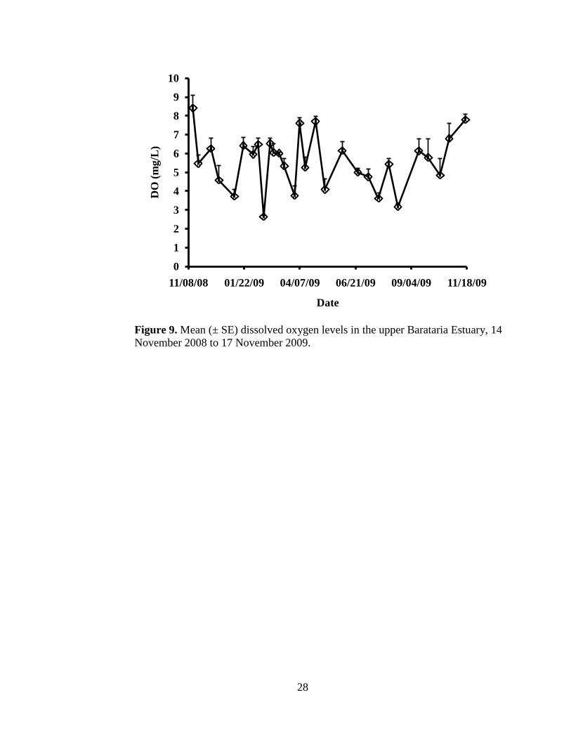
Figure 9. Mean (± SE) dissolved oxygen levels in the upper Barataria Estuary

from 14 November 2008 to 17 November 2009. ……………………28

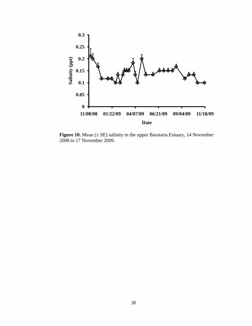
Figure 10. Mean (± SE) salinity in the upper Barataria Estuary from 14

November 2008 to 17 November 2009. ……………………………..30

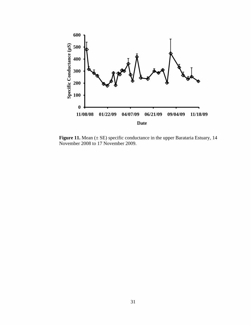
Figure 11. Mean (± SE) specific conductance in the upper Barataria Estuary from

14 November 2008 to 17 November 2009. ………………………….31

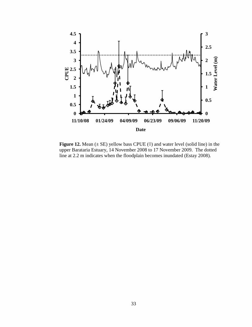
Figure 12. Mean (± SE) yellow bass CPUE (◊) and water level (solid line) in the

upper Barataria Estuary from 14 November 2008 to 17 November

2009. …………………………………………………………………33

viii

Figure 13. Photoperiod for the 15th of each month from January 2009 to June

2009 for Thibodaux, Louisiana, Dyersburg, Tennessee, Clear Lake

City, Iowa, and Madison, Wisconsin. .………………………………34

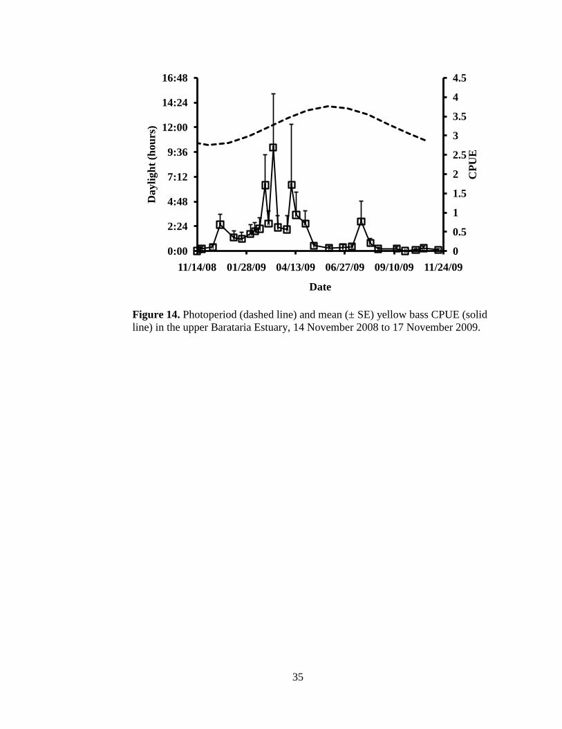
Figure 14. Photoperiod (dashed line) and mean (± SE) yellow bass CPUE (solid

line) in the upper Barataria Estuary from 14 November 2008 to 17

November 2009. ……………………………………………………..35

Figure 15. Total length frequency distributions of male (N = 769; dark bars) and

female (N = 292; open bars) yellow bass collected 14 November 2008

to 17 November 2009 from the upper Barataria Estuary. …………...36

Figure 16. Length-weight relationship data for male and female yellow bass

combined, collected from the upper Barataria Estuary from 14

November 2008 to 17 November 2009. ……………………………..37

Figure 17. Age frequency for yellow bass collected from the upper Barataria

Estuary 14 November 2008 to 17 November 2009. ………………...38

Figure 18. Mean (± SE) total length at age for male (□) and female (◊) yellow

bass collected from the upper Barataria Estuary 14 November 2008 to

17 November 2009. ………………………………………………….40

Figure 19. Mean (± SE) GSI for male (solid line) and female (dashed line) yellow

bass collected from the upper Barataria Estuary, 14 November 2008 to

17 November 2009. ………………………………………………….41

Figure 20. Mean (± SE) GSI for male (open square dashed line) and female (open

diamond dotted line) and mean (± SE) CPUE for yellow bass collected

in the upper Barataria Estuary, 14 November 2008 to 17 November

2009. …………………………………………………………………42

Figure 21. Mean (± SE) monthly female yellow bass GSI collected from the

upper Barataria Estuary 14 November 2008 to 17 November 2009.

………………………………..………………………………………43

Figure 22. Percent of “developing” (grey bar), “spawning capable/actively

spawning” (black bar) and “regressing/regenerating” (open bar)

developmental stages of male yellow bass collected 14 November

2008 to 17 November 2009, from the upper Barataria Estuary.

………………………………………………………………………..44

Figure 23. Histological section of a “spawning capable/actively spawning” male

yellow bass (TL = 209 mm) testis with spermatozoa throughout

lumens and sperm ducts collected on 17 February 2009, in the upper

Barataria Estuary. ……………………………………………………45

ix

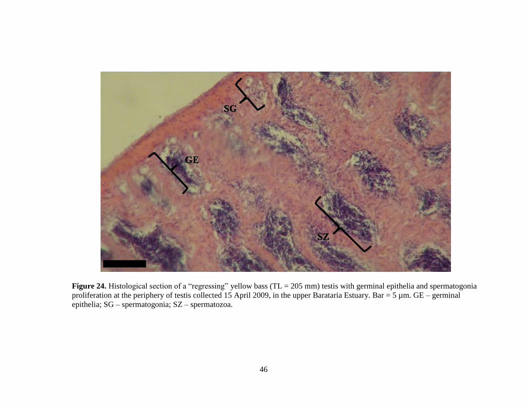
Figure 24. Histological section of a “regressing” male yellow bass (TL = 205

mm) testis with germinal epithelia and spermatogonia proliferation at

the periphery collected 15 April 2009, from the upper Barataria

Estuary. ……………………………………………………………...46

Figure 25. Histological section of a “regenerating” male yellow bass (TL = 200)

testis with small lumens and spermatogonia throughout collected 03

June 2009, from the upper Barataria Estuary. ……………………….47

Figure 26. Histological section of a “developing” male yellow bass (TL = 195

mm) testis with spermatogonia proliferation in spermatocysts at the

periphery collected 08 December 2008, from the upper Barataria

Estuary. ……………………………………………………………...48


spawning” (black bar) and “regressing/regenerating” (open bar)

developmental stages of female yellow bass collected from 14

November 2008 – 17 November 2009, from the upper Barataria

Estuary. ……………………………………………………………...49

Figure 28. Histological section of a “spawning capable” female yellow bass (TL

= 218 mm) ovary with a >24 hour post-ovulatory follicle complex

collected 04 March 2009, from the upper Barataria Estuary. ……….50

Figure 29. Histological section of an “actively spawning” female yellow bass (TL

= 235 mm) ovary with oocytes undergoing lipid coalescence and

germinal vesicle migration collected on 10 Apr 2009, from the upper

Barataria Estuary. …..……………………………………….……….51

Figure 30. Histological section of a “regressing” female yellow bass (TL = 230

mm) ovary with mostly atretic oocytes collected on 18 March 2009,

from the upper Barataria Estuary. …………………………………...53

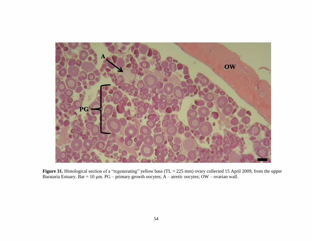
Figure 31. Histological section of a “regenerating” female yellow bass (TL = 225

mm) ovary collected 15 April 2009, from the upper Barataria Estuary.

………………………………………………………………………..54

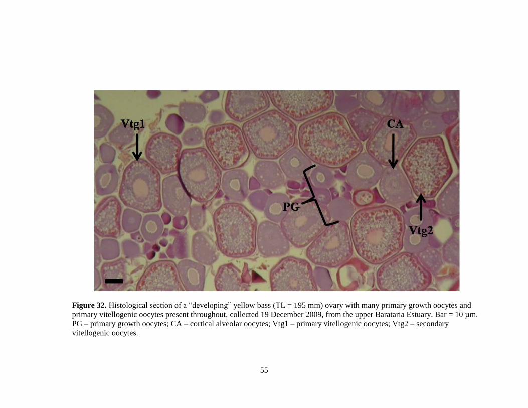
Figure 32. Histological section of a “developing” female yellow bass (TL = 195

mm) ovary collected 19 December 2008. …………………………...55

x

LIST OF TABLES

Table 1. Tissue processing procedure for histological preparation of yellow bass

gonad samples. ……………………………………………………….17

Table 2. Staining procedure for histological preparation of yellow bass gonad

samples. ………………………………………………………………18

Table 3. Reproductive classification system for male and female fishes

according to histological characteristics of gonads (modified from

Brown-Peterson et al. 2007). …………………………………………19

Table 4. Description of reproductive classification system for male yellow bass

according to histological characteristics of gonads (modified from


Table 5. Description of reproductive classification system for female yellow

bass according to histological characteristics of gonads (modified from


Table 6. Total number of each species of fish collected from the upper Barataria

Estuary 14 November 2008 to 17 November 2009. ………………….25

Table 7. Regression parameter estimates, standard errors, t-values, and P-values

from multiple regression analysis comparing CPUE to dissolved

oxygen (mg/L), temperature (°C), and specific conductance (µS).

…….……………………………………..……………………………32

1

INTRODUCTION

First described by Jordan and Eigenmann (1887), the yellow bass Morone

mississippiensis is a member of the family Moronidae with striped bass M.

saxatilis, white bass M. chrysops, and white perch M. americana. The specific

epithet is derived from the name Mississippi. Yellow bass are found in the

Mississippi River and its drainage basin from Minnesota to Louisiana and western

Iowa to eastern Tennessee (Figure 1; Douglas 1974; Lee et al. 1980; Page and

Burr 1991). Moronids are referred to as temperate basses, to be separated from

black bass species such as the largemouth bass Micropterus salmoides which is a

member of the sunfish family Centrachidae. Temperate basses include freshwater

(M. mississippiensis and M. chrysops), anadromous (M. saxatilis), and euryhaline

(M. americana) species (Mettee et al. 1996; Etnier and Starnes 2001).

Until recently, Morone spp. were listed in the family Percichthyidae and

grouped with many species from throughout North and South America, Europe,

Australia, Africa, and Asia (Page and Burr 1991; Etnier and Starnes 2001). In

1984, Johnson removed Morone spp., Dicentrarchus spp., Lateolabrax and

Coreoperca spp. from Percichthyidae and placed them into Moronidae.

Throughout the 1800s and early 1900s scientists debated the validity of the genus

Morone, proving and debating its separation from Percichthyidae many times

(reviewed in Whitehead and Wheeler 1966). The genus Morone was first

proposed by Mitchill (1814).

Yellow bass are moderately deep bodied fish with a terminal mouth, light

olive to yellowish color, 5-7 dark lateral stripes, which are usually broken and off

2

Figure 1. Distribution of yellow bass in the United States. The bold outline

delineates the Mississippi River drainage basin. The dark shaded region indicates

the native range for yellow bass (Adapted from Lee et al. 1980 and Page and Burr

1991).

3

set above the front of the anal fin, and often have yellow eyes (Figure 2; Smith

1979; Hubbs et al. 1991; Mettee et al. 1996; Ross 2001). The second and third

anal spines are nearly equal in length (Hubbs et al. 1991). The dorsal, caudal and

anal fins are dark, and the pectoral and pelvic fins are usually clear or white (Page

and Burr 1991; Ross 2001). The yellow bass can be separated from other

members of the Morone family by the lack of a tooth patch on their tongue and

the membrane that connects the two dorsal fins (Cook 1959; Hubbs et al. 1991).

The reported maximum size of adult yellow bass is 275 mm total length (TL) and

0.5 kg in weight (Burgess 1978; Boschung and Mayden 2004). According to Lee

et al. (1980) and Pflieger (1997), the maximum lifespan of yellow bass is six

years; however, yellow bass up to age eight have been collected in Clear Lake,

Iowa (Carlander 1997).

Yellow bass are a schooling species most commonly found in backwater

pools and oxbows of the river systems they inhabit (Driscoll and Miranda 1999;

Etnier and Starnes 2001). Harlan and Speaker (1956), Cook (1959), and Becker

(1983) listed the yellow bass as a game fish because of its feisty nature and wide

range of lure acceptance. Yellow bass meat is firm, white, flaky and is often

considered superior to white bass meat (Becker 1983). Several states encourage

the harvest of yellow bass to reduce angling pressure on other fish populations

residing in the same areas, yet many anglers tend to disregard them while trying

to land the larger white and striped basses (Pflieger 1997; Ross 2001).

In Tennessee and Wisconsin male and female yellow bass matured at ages

two and three, respectively (Priegel 1975; Carlander 1997). Males from Clear

4

Figure 2. Female yellow bass (TL=263 mm) collected 23 January 2009 from the

upper Barataria Estuary, Louisiana (photograph by Cynthia Fox).

5

Lake, Iowa matured at age two, but females matured at age four (Carlander 1997).

Throughout their range, yellow bass spawn in large streams over gravel substrate

during April and May (Bulkley 1970; Mettee et al. 1996), but the spawning

season can extend into June in the northernmost reaches of the yellow bass range

(Becker 1983). Yellow bass typically migrate upstream to spawn in waterways

that flow into the lakes where they reside. Similar to white crappie Pomoxis

annularis, lake sturgeon Acipenser fulvescens, and channel catfish Ictalurus

punctatus, male yellow bass migrate upstream to the spawning grounds prior to

females (Becker 1983; Ross 2001; Boschung and Mayden 2004).

Spawning activity in fish can be triggered by endogenous and exogenous

cues. Photoperiod and temperature are frequently the strongest environmental

cues that induce physiological and behavioral responses in fish. The

hypothalamus receives melatonin released from the pineal gland which stimulates

the pituitary gland to release gonadotropins (Jameson 1988). Common

gonadotropins in fish are called gonadotropin hormones (GtH) I and II (Lin et al.

2004). These hormones function similarly to the follicle-stimulating hormone

(FSH) and the luteinizing hormone (LH) in mammals (Jameson 1988; Patiño and

Sullivan 2002; Lin et al. 2004). Gonadotropins travel to the gonads and stimulate

the release of estrogen or testosterone (Jameson 1988). In females, estrogen then

travels to the liver where it initiates the production of vitellogenin (Vtg; Specker

and Sullivan 1994). Vtg is then transported by the bloodstream back to the ovary

where it is taken up by growing oocytes (Mommsen and Walsh 1988) in

preparation for maturation and spawning.

6

Yellow bass spawning in Iowa begins when water temperature reaches

approximately 18°C (Bulkley 1970) with the most intense spawning occurring

between 20-22°C (Becker 1983). Spawning occurs among one female and one to

several males (Burnham 1909; Mettee et al. 1996). As described by Burnham

(1909), yellow bass females lie on their side and release eggs towards the male

who remains right-side up and fertilizes the eggs as they are released. Female

yellow bass do not release their entire egg complement in one spawning attempt,

because all of the eggs do not mature at the same time (Burnham 1909; Bulkley

1970) leading to their as asynchronous batch spawners (Grier 2009). Yellow bass

eggs are semi-adhesive and hatch within 4-6 days of fertilization at 21°C (Ross

2001). The yolk sac contents are absorbed within 4 days and the fry begin

exogenous feeding and aggregate in schools according to fish size (Burnham

1909).

Yellow bass are one of many species found in the Barataria Estuary (Lantz

1970). Throughout their range, yellow bass initiate a pre-spawn migration to

preferred spawning habitats as temperatures approach 18°C (Bulkley 1970).

Similarly, gizzard shad migrate to the upper reaches of the Barataria Estuary to

spawn when temperatures reach 17-22°C, resulting in a much higher gizzard shad

abundance than during other times of the year (Fontenot et al. in press). As with

gizzard shad, yellow bass abundance in the UBE may be seasonal and related to

spawning activity. Few yellow bass have been collected from the Barataria

Estuary(Fontenot 2006; Davis 2006; Dyer 2007) and their ecological role within

the UBE has not been described.

7

Figure 3. The Barataria Estuary (shaded region) in southeast Louisiana.

8

The Barataria Estuary is bordered by Bayou Lafourche to the west and the

Mississippi River to the east (Figure 3), and is composed of interconnected lakes,

bayous, canals, cypress-tupelo swamps, bottomland hardwood forests, freshwater

marsh, intermediate marsh, brackish marsh, and salt marsh (Braud et al. 2006).

The main riverine conduit source of the upper reaches of the estuary is Bayou

Chevreuil, which drains much of the area into Lac des Allemands (Figure 4). For

several hundred years the Barataria Estuary was inundated by an annual spring-

time Mississippi River flood pulse. However, flood protection levee construction

has cut off the upper estuary from the Mississippi River (Sklar and Conner 1979;

Inoue et al. 2008). As a result, the water level in the upper estuary is a function of

local precipitation and wind direction (Hopkins and Day 1987; Inoue et al. 2008).

The lack of annual floodplain inundation may negatively impact spawning of

many riverine fish species (Bayley 1995), such as bowfin (Davis 2006).

However, the lack of a flood pulse does not appear to affect gizzard shad

spawning activity (Jackson 2009; Fontenot et al. in press).

Low oxygen levels can negatively affect aquatic species (Suthers and Gee

1986; Kramer 1987; Fontenot et al. 2001; Killgore and Hoover 2001). Based on

oxygen level, bodies of water can be classified as normoxic (DO > 2.0 mg/L),

hypoxic (DO ≤ 2.0 mg/L), or anoxic (DO = ≤ 0.02 mg/L; Estay 2008). Hypoxic

conditions in the UBE can range from a few days to several weeks (Estay 2008)

and can affect blue crab abundance (Dantin et al. in press). Hypoxic conditions

are typical of the high water period in active large river floodplains representing a

normal component of the yearly flood pulse cycle (Junk et al. 1989; Bayley

9

Figure 4. Major waterways (solid lines) and roadways (dashed lines) of the upper

Barataria Estuary, Louisiana.

10

1995). However, hypoxic conditions in the UBE are most likely related to rain

events (Estay 2008), and are not predictable. The unpredictable occurrence of

hypoxic conditions without being coupled to a seasonal flood pulse in the UBE

may disrupt the distribution and abundance of the fishes in the system.

The gonadosomatic index measures the cyclic changes in gonad weight in

relation to total fish weight, and can be used to determine spawning periods

(Nieland and Wilson 1993; Jons and Miranda 1997; Smith 2008). An increase in

GSI suggests an approaching spawning season, and a decrease suggests spawning

has occurred. Gonad histology is the microscopic examination of gonads and is

used to classify individuals into specific reproductive stages. Combining GSI

with histological analysis enhances the ability to determine if fish are spawning in

the immediate area.

Using histology, both male and female fish can be separated into one of

six reproductive stages (Brown-Peterson et al. 2007). Individuals can be

classified as “immature” (not capable of spawning), “developing” (gonads

developing but not capable of spawning), “spawning capable” (capacity to spawn

this season), “actively spawning” (active or recent spawning), “regressing” (post-

spawning), or “regenerating” (post-spawning and recovering; Brown-Peterson et

al. 2007). Histology has been used to assess gonad development and to describe

the reproductive cycle of fish (Blazer 2002; Lowerre-Barbieri et al. 2003). In

addition to GSI, Smith (2008) used gonad histology to more accurately describe

the reproductive cycle of spotted gar by identifying gonad development through

time.

11

Fish age can be estimated using hard structures such as otoliths, scales,

spines or fin rays (Welch et al. 1993; Soupir et al. 1997) according to species

specific characteristics. In striped bass and white bass, otoliths have been more

accurate than scales for age determination (Soupir et al. 1997; Secor et al. 1995;

Welch et al. 1993). Basic life history characteristics of fishes such as annual

growth rates, difference in growth rates between the sexes, age of maturity, and

year class strength require age data. In some fish species, a large percentage of

the population will consist of one or two year classes (Jennings et al. 2001) as

seen in Atlantic herring Clupea harengus and Atlantic cod Gadus morhua (Hjort

1914). Also, monitoring changes in population age structure allows for

assessment of how environmental or management changes affect the population.

Few studies have been published on yellow bass life history south of

Tennessee (Schoffman 1958; Darnell 1961; Van Den Avyle and Higginbotham

1983; Driscoll and Miranda 1999). Most information pertaining to yellow bass in

the southeast has either been related to diet ecology or the commercial

hybridization of yellow bass with white and striped bass (Darnell 1961; Wolters

and DeMay 1996; Bosworth et al. 1998; Driscoll and Miranda 1999). In

Louisiana, yellow bass have been captured for hybridization and trophic level

studies (Darnell 1961; Wolters and DeMay 1996); however their life history

characteristics have not been documented.

The goal of this study was to describe the seasonal abundance and life

history characteristics of the yellow bass population in the upper Barataria

Estuary. The specific objectives of this study were to:

12

1. Quantify seasonal abundance of yellow bass,

2. Determine sex specific age and growth rates,

3. Determine sex specific gonadosomatic index,

4. Use histological techniques to describe seasonal gonad development,

and to confirm spawning, and

5. Determine the relationships between dissolved oxygen (DO; mg/L),

salinity (ppt), specific conductance (µS), temperature (°C), water level

(m), and photoperiod (hours of daylight) and yellow bass abundance.

13

METHODS

Field Sampling

To describe the yellow bass population in the upper Barataria Estuary,

yellow bass were collected from three sites in Lac des Allemands (Figure 5) and

three sites in Bayou Chevreuil (Figure 5) from 14 November 2008 to 17

November 2009, using monofilament gill nets. Sampling occurred biweekly from

mid-April through January and weekly from February through mid-April. Three

separate individual 22 m long, 1.8 m deep, 25.4 mm and 35 mm bar mesh nets,

and a single 22 m dual mesh net (first section: 11 m long, 1.8 m deep, 25.4 mm

bar mesh; second section: 11 m long, 1.8 m deep, 51 mm bar mesh) were

deployed for approximately three hours at each site. Nets in the bayou were set at

a 45º angle from the shore pointing downstream, and nets set in the lake were set

parallel to the western shore. At each sample site dissolved oxygen (DO, mg/L),

specific conductance (µS), temperature (ºC), and salinity (ppt) were measured 0.3

m below the surface of the water using a handheld oxygen-conductivity-salinity-

temperature meter (Yellow Springs Instruments, Yellow Springs, Ohio). Water

level (m) data was obtained from the USGS monitoring site #07380401 in the St.

James Canal (Figure 5). To compare photoperiod among known spawning periods

for yellow bass, photoperiod data for the 15th

of each month from January 2009

through July 2009 were obtained from the United States Naval Observatory

(http://aa.usno.navy.mil/) for Thibodaux, Louisiana, Dyersburg, Tennessee, Clear

Lake City, Iowa, and Madison, Wisconsin.

All yellow bass were kept on ice in separate labeled containers for each

14

Figure 5. Location of the six study sites located in Lac des Allemands (sites 1-3)

and Bayou Chevreuil (sites 4-6). GPS coordinates for each site are: Site 1:

29°54’22.7”N, 90°35’11.1”W; Site 2: 29°54’08.0”N, 90°35’37.7”W; Site 3:

29°53’44.9”N, 90°35’52.7”W; Site 4: 29°53’36.9”N, 90°40’50.5”W; Site 5:

29°55’46.9”N, 90°44’51.0”W; Site 6: 29°55’21.3”N, 90°47’06.5”W. Bar = 7.7

km.

15

net and transported to the Bayousphere Research Laboratory at Nicholls State

University for processing. All other species collected were recorded and released

on site. Catch per unit effort (CPUE) was calculated for each net by dividing the

number of yellow bass caught in the net by the number of hours the net was

deployed (# fish/# hours). The mean CPUE for each net type within each habitat

was calculated. Although net mesh sizes were different, the same net

combinations were used at each site, therefore the mean CPUE for all nets at each

site was combined for an overall site CPUE. Only one yellow bass (TL = 215

mm, weight =152 g) was collected in the 51 mm bar mesh, so that net size was

not included in any analyses.

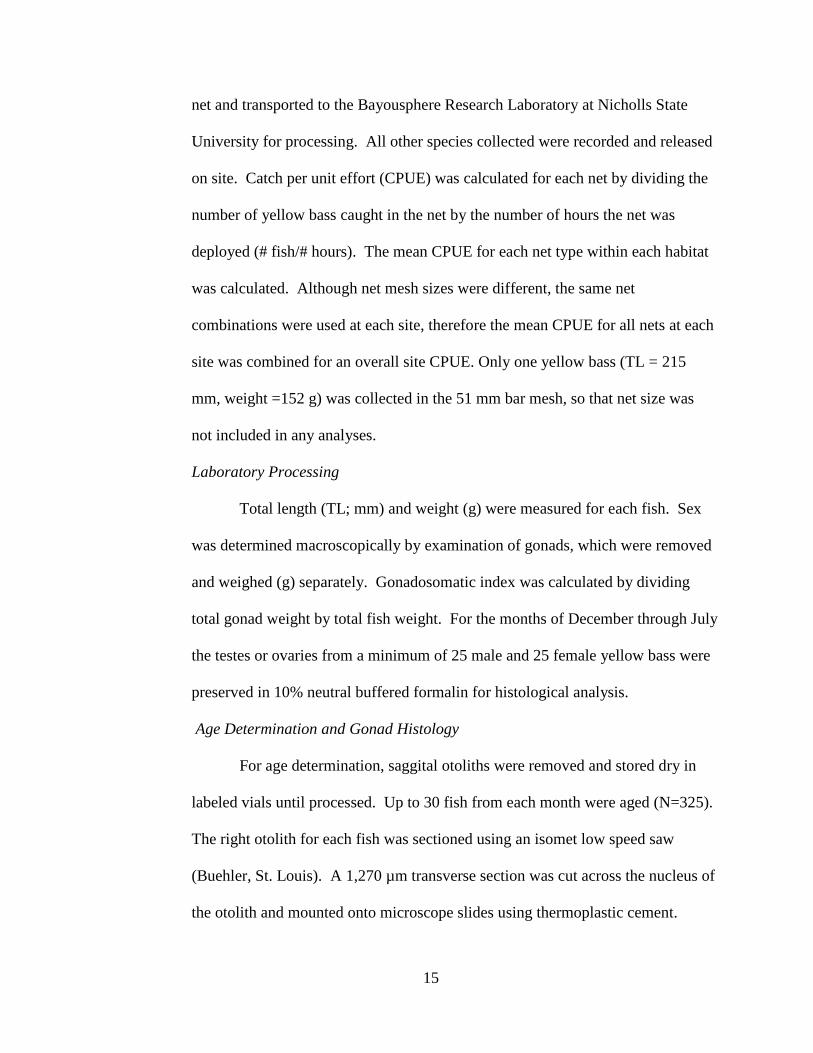
Laboratory Processing

Total length (TL; mm) and weight (g) were measured for each fish. Sex

was determined macroscopically by examination of gonads, which were removed

and weighed (g) separately. Gonadosomatic index was calculated by dividing

total gonad weight by total fish weight. For the months of December through July

the testes or ovaries from a minimum of 25 male and 25 female yellow bass were

preserved in 10% neutral buffered formalin for histological analysis.

Age Determination and Gonad Histology

For age determination, saggital otoliths were removed and stored dry in

labeled vials until processed. Up to 30 fish from each month were aged (N=325).

The right otolith for each fish was sectioned using an isomet low speed saw

(Buehler, St. Louis). A 1,270 µm transverse section was cut across the nucleus of

the otolith and mounted onto microscope slides using thermoplastic cement.

16

After mounting, otolith sections were ground with 600 grit wet/dry sandpaper

until smooth then polished with 800 grit wet/dry sandpaper for approximately

twenty seconds. Two readers independently viewed otolith sections coated with

immersion oil using a dissecting microscope (Olympus SZX12) at varying

magnifications. Lengths of the fish were not known by the readers and any

discrepancies were discussed among the readers until an age was agreed on.

Histological methods followed the methods of Brown-Peterson et al.

(2007). Samples from the center of the gonads were cut (approximately 5 mm

thick), placed in labeled tissue cassettes, stored in 75% ethanol for up to five days

and sent to McNeese State University, Lake Charles, Louisiana for processing.

The tissues were dehydrated in ascending grades of alcohol, cleared in xylene and

infiltrated with paraffin (Table 1). Post-infiltration, the tissues were embedded

and 10μm sections were made using a microtome. Slides were stained using

hematoxylin and eosin and coverslipped (Table 2). Each slide was viewed using a

compound light microscope (Nikon Eclipse E600) at 20, 40, 100, or 200X

magnification. A modification of the Brown-Peterson et al. (2007) reproductive

classification system (Table 3) was used to provide descriptions specific to male

(Table 4) and female (Table 5) yellow bass gonad histology. For histological

analyses of both sexes, the “spawning capable” and “actively spawning” stages

were combined (Smith 2008). In females, these stages occur intermittently until a

female finishes spawning for that year. In males, the two stages are histologically

indistinguishable and can only be separated by the observation of free flowing

milt before dissection.

17

Table 1. Tissue processing procedure for histological preparation of yellow bass

gonad samples.

Station Treatment Time

1 75% Alcohol Up to 5 days

2 75% Alcohol 30 min







9 Xylene in Vacuum 30 min

10 Xylene in Vacuum 30 min

11 Paraffin in Vacuum 30 min

12 Paraffin in Vacuum 30 min

13 Imbed with Paraffin 2-3 min

14 Microtome Variable

15 Warm Water Bath 5 min

16 Stretching Block Overnight

18

Table 2. Staining procedure for histological preparation of yellow bass gonad

samples. Acid water – 3% glacial acetic acid in water, Ammonia water – 3%

ammonium hydroxide in water. A – Agitation, D – Dip, W – Wash, S – Soak.

Station Reagent Action Time/Number

1 Xylene A 3-6 min

2 Xylene A 3-6 min

3 100% Alcohol D 20-30

4 100% Alcohol D 20-30

5 95% Alcohol D 20-30

6 95% Alcohol D 20-30

7 Water W 3-5 min

8 Hematoxylin S 2 min

9 Water W 3 min

10 Acid Water D 1

11 Water W 3 min

12 Ammonia Water D 3

13 Water W 3 min

14 70% Alcohol D 20-30

15 Eosin S 2 min

16 95% Alcohol D 20

17 95% Alcohol D 20

18 100% Alcohol D 20-30

19 Xylene D 20

Coverslip 1 min

Set Overnight

19

Table 3. Reproductive classification system for male and female fishes according to histological characteristics of gonads (modified

from Brown-Peterson et al. 2007). Female “regressing” stage was modified to include vitellogenic and cortical alveolar oocytes. PGO

– primary growth oocytes, CAO – cortical alveolar oocytes, VTGO – vitellogenic oocytes, POF – post-ovulatory follicles, GVM –

germinal vesicle migration, GVBD – germinal vesicle breakdown, SG – spermatogonia, CY – spermatocysts, SC – spermatocytes, ST

– spermatids, SZ – spermatozoa, GE – germinal epithelia.

Stage Male Female

Immature Small testes, only primary SG, no lumens in lobules. Only oogonia and PGO present. Usually no atresia.

Developing Initiation of spermatogenesis and formation of CY.

Secondary SG, primary SG, secondary SC, ST, and

SZ can be present in CY. No SZ in lumens of lobules

or sperm ducts. GE continuous.

PGO, CAO, early VTGO, and mid VTGO may be

present. No POF. Some atresia can be present.

Spawning

Capable

SZ in lumens of lobules and/or sperm ducts. All

stages of spermatogenesis (SG, SC, and ST) can be

present. CY throughout testis. GE continuous or

discontinuous. Histologically undistinguishable from

“actively spawning” phase.

VTGO predominant. Some atresia and old POF may

be present. Less-developed oocytes often present.

Actively

Spawning

SZ in lumens of lobules and/or sperm ducts. All

stages of spermatogenesis (SG, SC, and ST) can be

present. CY throughout testis. GE continuous or

discontinuous. Histologically undistinguishable from

“spawning capable” phase.

Ovulating (spawning) or approximately 12 hours

prior to or after spawning as indicated by either

GVM, GVBD/hydrated oocytes, or POF < 12 hours

old. Atresia of late VTGO or hydrated oocytes may

be present.

Regressing Residual SZ in lumens of lobules and sperm ducts.

Widely scattered CY near periphery containing ST.

SG proliferation and GE regeneration common in

periphery of testis.

Atresia present (any stage). Majority of VTGO

undergoing early atresia. Less-developed oocytes

often present. VTGO or CAO can be present. POF

may be present.

Regenerating No CY. Lumens of lobules small or nonexistent.

Proliferation of primary, occasionally secondary, SG

throughout testis. Residual SZ may be present in

lumens of lobules and sperm ducts.

Only oogonia and PGO present. Muscle bundles,

enlarged blood vessels, thick ovarian wall and/or late

atresia may be present.

20

Table 4. Description of reproductive classification system for male yellow bass

according to histological characteristics of gonads (as modified from Brown-

Peterson et al. 2007). SG – spermatogonia, CY – spermatocysts, ST – spermatids,

SZ – spermatozoa, GE – germinal epithelium.

Stage Description

Immature Only primary SG present. No lumens.

Developing Continuous GE throughout testis. Spermatogenesis begins

giving rise to the formation of CY. CY are clusters of cells in

the same stage of spermatogenesis. CY may contain

secondary SG, primary SC, secondary SC, ST and SZ. As SG

develop into SZ, each stage of cells become smaller, increase

in number, and stain darker purple. SZ can be separated from

ST by the appearance of a bright pink tail on SZ. No SZ will

be in lumen.

Spawning

Capable

SZ released and scattered throughout lumens and sperm

ducts. Some CY present throughout testis. CY may contain

all stages of spermatogenesis (SG, SC, and ST). GE can be

continuous or discontinuous. Histologically undistinguishable

from “actively spawning” stage. However, if milt does not

flow from vent with gentle squeeze, fish can be classified into

this stage.

Actively

Spawning

SZ released and scattered throughout lumens and sperm

ducts. Some CY present and may contain SG, SC, and ST.

GE may be continuous or discontinuous. Histologically

undistinguishable from “spawning capable” stage. However,

if milt flows from vent with gentle squeeze, fish can be

classified into this stage.

Regressing Residual SZ present in lumens. Some CY containing ST

scattered near periphery. Primary SG begins forming at

periphery as GE regeneration also begins.

Regenerating No CY present. Lumens are small and difficult to see.

Primary SG dominant with some secondary SG present.

Residual SZ may be present.

21

Table 5. Description of reproductive classification system for female yellow bass

according to histological characteristics of gonads (as modified from Brown-

Peterson et al. 2007). PG – primary growth oocytes, CA – cortical alveolar

oocytes, Vtg – vitellogenic oocytes, POC – post-ovulatory follicle complex, OM –

oocyte maturation, GVM – germinal vesicle migration, FOM – final oocyte

maturation, MA – macrophage aggregates.

Stage Description

Immature Only PG present. Usually no atresia. Thin ovarian wall.

Developing PG present and stained dark purple. CA larger than PG and

stained light purple. Cortical alveoli are small dark purple

spheres that form a circle inside the CA. Primary Vtg are

similar to CA (in size) but contain small dark pink granules and

white yolk oil droplets. Granules line outer edge of oocyte

while droplets surround nucleus. Atresia may be present

appearing as “empty holes,” indicating previous location of

fatty tissue. Some secondary Vtg may be present.

Spawning

Capable

Tertiary Vtg prominent. Secondary and primary Vtg common,

CA present. Secondary Vtg are larger and contain more yolk

than early Vtg with a dark pink vitelline envelope. Thin layer

of thecal cells surrounds all Vtg oocytes, but may be difficult to

distinguish between oocytes. Ovarian wall will start thinning.

Old (> 24 h) small POCs present and appear grainy and folded.

Actively

Spawning

OM present with lipid and yolk coalescence occurring with

GVM. Tertiary Vtg prominent and larger than Secondary Vtg.

Some FMOs can be present with fused yolk that is stained pink

and looks smooth or layered. Vitelline envelope will be thick

and dark pink. Some new (<24 h) POCs, atresia and PGs may

be present.

Regressing Atresia dominant. Some FMOs, POCs, and PGs scattered

throughout ovary. MA present appearing yellowish- brown.

Some Vtg and CA oocytes present.

Regenerating Only PGs present. Blood vessels enlarged. Some late stage

atresia and MA may be present. Thick ovarian wall.

22

Statistical Analyses

Analysis of variance was used to determine if DO, temperature, specific

conductance, or CPUE differed among sites. Multiple regression analysis was

used to determine the relationships among CPUE and DO temperature, salinity,

and specific conductance. Analysis of variance was used to compare age specific

size difference between the sexes. Analysis of variance was used to compare

CPUE and sex specific GSI among months and was followed by Tukey’s post hoc

analysis. All statistical inference were based on alpha = 0.05.

23

RESULTS

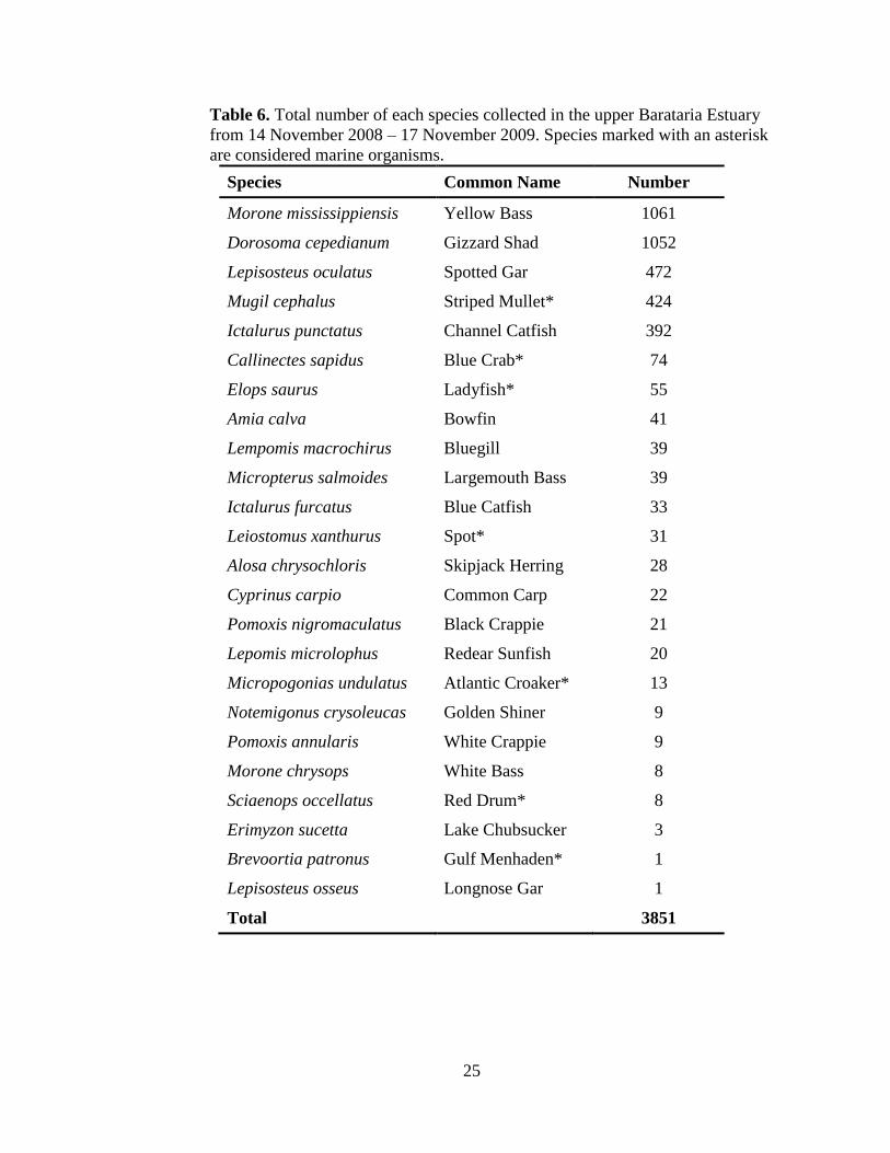
A total of 1,061 yellow bass were collected from 14 November 2008 to 17

November 2009 from the upper Barataria Estuary and the male:female ratio was

2.63:1 (male N = 769; female N = 292). Males made up more than 70% of the

catch for February, March and April (Figure 6). In addition to yellow bass,

twenty-three other species were collected, including seven marine species (Table

6). Yellow bass CPUE increased during the winter, peaked in early spring, and

declined and remained low throughout the summer and the fall, with the

exception of a small increase on 22 July 2009. The greatest peak in abundance

occurred on 10 March 2009 (Appendix I) after water temperature reached 18 -

22°C (Figure 7). Yellow bass abundance was greatest (P = 0.0003) during their

spawning season (February through April; Figure 8) compared to months they are

not spawning; however, mean CPUE did not differ among the six sites (P =

0.6711).

Site specific dissolved oxygen measurements ranged from 0.7 to 14.3

mg/L (Appendix II) with an average of 7.8 ± 1.4 mg/L (mean ± SE). Mean

dissolved oxygen levels did not differ among the six sites (P = 0.9985; Figure 9).

Site specific temperature measurements ranged from 10.4 to 33.8°C (Appendix II)

with an average of 22.4 ± 6.3°C. Temperatures fluctuated seasonally with the

highest mean temperature (32.1°C) occurring in June and the lowest (11.1°C)

occurring in January (Figure 7) with no difference among the sites (P = 0.9687).

Site specific salinity measurements ranged from 0.1 to 0.3 ppt (Appendix II) and

averaged 0.14 ± 0.03 ppt. Salinity remained fairly constant among all six sites

24

Figure 6. Percent of monthly catch of male (N = 769; dark bar) and female (N =

292; open bar) yellow bass collected 14 November 2008 to 17 November 2009,

from the upper Barataria Estuary. Numbers above columns indicate the total

number of fish collected each month.

0.0

0.2

0.4

0.6

0.8

1.0

Nov Dec Jan Feb Mar Apr May Jun Jul Aug Sept Oct

% o

f C

atc

h

Month

56 49 224 279 342 9 11 59 16 6 73

25

Table 6. Total number of each species collected in the upper Barataria Estuary

from 14 November 2008 – 17 November 2009. Species marked with an asterisk

are considered marine organisms.

Species Common Name Number

Morone mississippiensis Yellow Bass 1061

Dorosoma cepedianum Gizzard Shad 1052

Lepisosteus oculatus Spotted Gar 472

Mugil cephalus Striped Mullet* 424

Ictalurus punctatus Channel Catfish 392

Callinectes sapidus Blue Crab* 74

Elops saurus Ladyfish* 55

Amia calva Bowfin 41

Lempomis macrochirus Bluegill 39

Micropterus salmoides Largemouth Bass 39

Ictalurus furcatus Blue Catfish 33

Leiostomus xanthurus Spot* 31

Alosa chrysochloris Skipjack Herring 28

Cyprinus carpio Common Carp 22

Pomoxis nigromaculatus Black Crappie 21

Lepomis microlophus Redear Sunfish 20

Micropogonias undulatus Atlantic Croaker* 13

Notemigonus crysoleucas Golden Shiner 9

Pomoxis annularis White Crappie 9

Morone chrysops White Bass 8

Sciaenops occellatus Red Drum* 8

Erimyzon sucetta Lake Chubsucker 3

Brevoortia patronus Gulf Menhaden* 1

Lepisosteus osseus Longnose Gar 1

Total 3851

26

Figure 7. Mean (± SE) yellow bass CPUE (◊) and temperature (∆) in the upper

Barataria Estuary, 14 November 2008 to 17 November 2009. Dotted line at 18°C

indicates the temperature that spawning is reported to occur (Bulkley 1970).

0

5

10

15

20

25

30

35

0

0.5

1

1.5

2

2.5

3

3.5

4

4.5

11/08/08 01/22/09 04/07/09 06/21/09 09/04/09 11/18/09

Tem

pera

ture

(C

)

CP

UE

Date

27

Figure 8. Mean (± SE) yellow bass CPUE collected during the spawning

(February to April) and the non-spawning season (May to January; P = 0.0003) in

the upper Barataria Estuary from November 2008 and November 2009.

0

0.3

0.6

0.9

1.2

1.5

Spawning Non-Spawning

CP

UE

(# /

Net

-ho

ur)

Season

28

Figure 9. Mean (± SE) dissolved oxygen levels in the upper Barataria Estuary, 14

November 2008 to 17 November 2009.

0

1

2

3

4

5

6

7

8

9

10

11/08/08 01/22/09 04/07/09 06/21/09 09/04/09 11/18/09

DO

(m

g/L

)

Date

29

(Figure 10). Site-specific specific conductance values ranged from 115 to 879.7

µS (Appendix II) with an average of 280.1 ± 73.8 µS. There was no difference

among the mean specific conductance values of the six sites (P = 0.9975; Figure

11). Multiple regression analysis did not reveal a significant relationship between

CPUE and DO, temperature, or specific conductance (Table 7). Daily individual

water level measurements recorded by the USGS ranged from 1.36 to 2.38 m with

an average of 1.81 ± 0.21 m. There was no evidence of a flood pulse and water

level was not related to yellow bass abundance (Figure 12). Day length steadily

increased for all four locations from January through June and was similar among

locations in March (Figure 13); however, there was no correlation between CPUE

and photoperiod (Figure 14). Peak yellow bass abundance occurred when

photoperiod was at 12L:12D.

Yellow bass collected during this study ranged from 175 mm to 264 mm

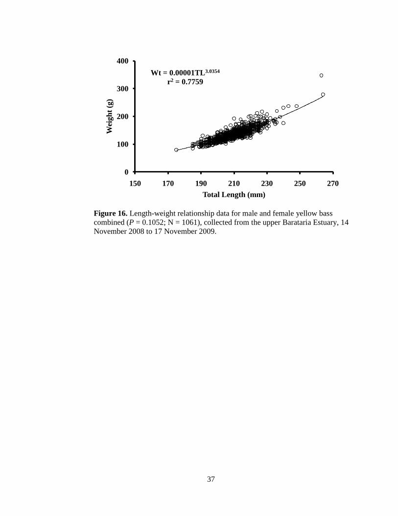
(Figure 15). Yellow bass weight ranged from 79.5 g to 347.5 g. Mean female

length (P = <0.0001) and weight (P = <0.0001) were larger than mean male

length and weight. There was no difference in the length-weight relationships (P

= 0.1052) between male and female yellow bass, therefore length and weight data

for the sexes were combined (Figure 16). The length-weight relationship for

yellow bass in the upper Barataria Estuary is described by:

WT = 0.00001TL3.0354

Fish age ranged from 1 to 4 years old but did not include any 3 year old

individuals. This population of yellow bass was dominated by two year old fish

(Figure 17). Because 95% of the fish aged were 2 years old, von Bertalanffy

30

Figure 10. Mean (± SE) salinity in the upper Barataria Estuary, 14 November

2008 to 17 November 2009.

0

0.05

0.1

0.15

0.2

0.25

0.3

11/08/08 01/22/09 04/07/09 06/21/09 09/04/09 11/18/09

Sali

nit

y (

pp

t)

Date

31

Figure 11. Mean (± SE) specific conductance in the upper Barataria Estuary, 14


0

100

200

300

400

500

600

11/08/08 01/22/09 04/07/09 06/21/09 09/04/09 11/18/09

Sp

ecif

ic C

on

du

ctan

ce (

µS

)

Date

32

Table 7. Regression parameter estimates, standard errors, t-values, and P-values

for multiple regression analysis comparing CPUE to dissolved oxygen (mg/L),

temperature (°C), and specific conductance (µS).

Variable Parameter

Estimate

Standard

Error t-value P-value

Dissolved

Oxygen 0.00293 0.03393 0.09 0.9312

Temperature -0.00551 0.01126 -0.49 0.6253

Specific

Conductance -0.00091 0.00075 -1.21 0.2283

33

Figure 12. Mean (± SE) yellow bass CPUE (◊) and water level (solid line) in the

upper Barataria Estuary, 14 November 2008 to 17 November 2009. The dotted

line at 2.2 m indicates when the floodplain becomes inundated (Estay 2008).

0

0.5

1

1.5

2

2.5

3

0

0.5

1

1.5

2

2.5

3

3.5

4

4.5

11/10/08 01/24/09 04/09/09 06/23/09 09/06/09 11/20/09

Wate

r L

evel

(m

)

CP

UE

Date

34

Figure 13. Photoperiod for the 15th of each month from January 2009 to June

2009 for Thibodaux, Louisiana, Dyersburg, Tennessee Clear Lake City, Iowa,

and Madison, Wisconsin. Data obtained for the United States Naval Observatory

(http://aa.usno.navy.mil/).

0:00

2:24

4:48

7:12

9:36

12:00

14:24

16:48

Jan Feb Mar Apr May Jun Jul

Dayli

gh

t (h

ou

rs)

Month

Louisiana Tennessee Iowa Wisconsin

35

Figure 14. Photoperiod (dashed line) and mean (± SE) yellow bass CPUE (solid

line) in the upper Barataria Estuary, 14 November 2008 to 17 November 2009.

0

0.5

1

1.5

2

2.5

3

3.5

4

4.5

0:00

2:24

4:48

7:12

9:36

12:00

14:24

16:48

11/14/08 01/28/09 04/13/09 06/27/09 09/10/09 11/24/09

CP

UE

Dayli

gh

t (h

ou

rs)

Date

36

Figure 15. Total length frequency distributions of male (N = 769; dark bars) and

female (N = 292; open bars) yellow bass collected 14 November 2008 to 17

November 2009 from the upper Barataria Estuary.

0

20

40

60

80

100

120

140

160

175

180

185

190

195

200

205

210

215

220

225

230

235

240

245

250

255

260

265

Nu

mb

er o

f F

ish

Total Length (mm)

37

Figure 16. Length-weight relationship data for male and female yellow bass

combined (P = 0.1052; N = 1061), collected from the upper Barataria Estuary, 14


Wt = 0.00001TL3.0354

r2 = 0.7759

0

100

200

300

400

150 170 190 210 230 250 270

Wei

gh

t (g

)

Total Length (mm)

38

Figure 17. Age frequency of yellow bass collected from the upper Barataria

Estuary, 14 November 2008 to 17 November 2009. Numbers above columns

indicate the total number of fish in that age class.

0

65

130

195

260

325

1 2 3 4

Nu

mb

er

Age (years)

320

1 40

39

growth parameters were not calculated.. Female yellow bass were larger than

male yellow bass for ages 2 and 4 (Figure 18).

As with CPUE, yellow bass GSI increased during the winter, peaked in

early spring, and declined and remained low throughout the summer and the fall.

Peak GSI occurred on 03 February 2010, for both males and females (Figure 19).

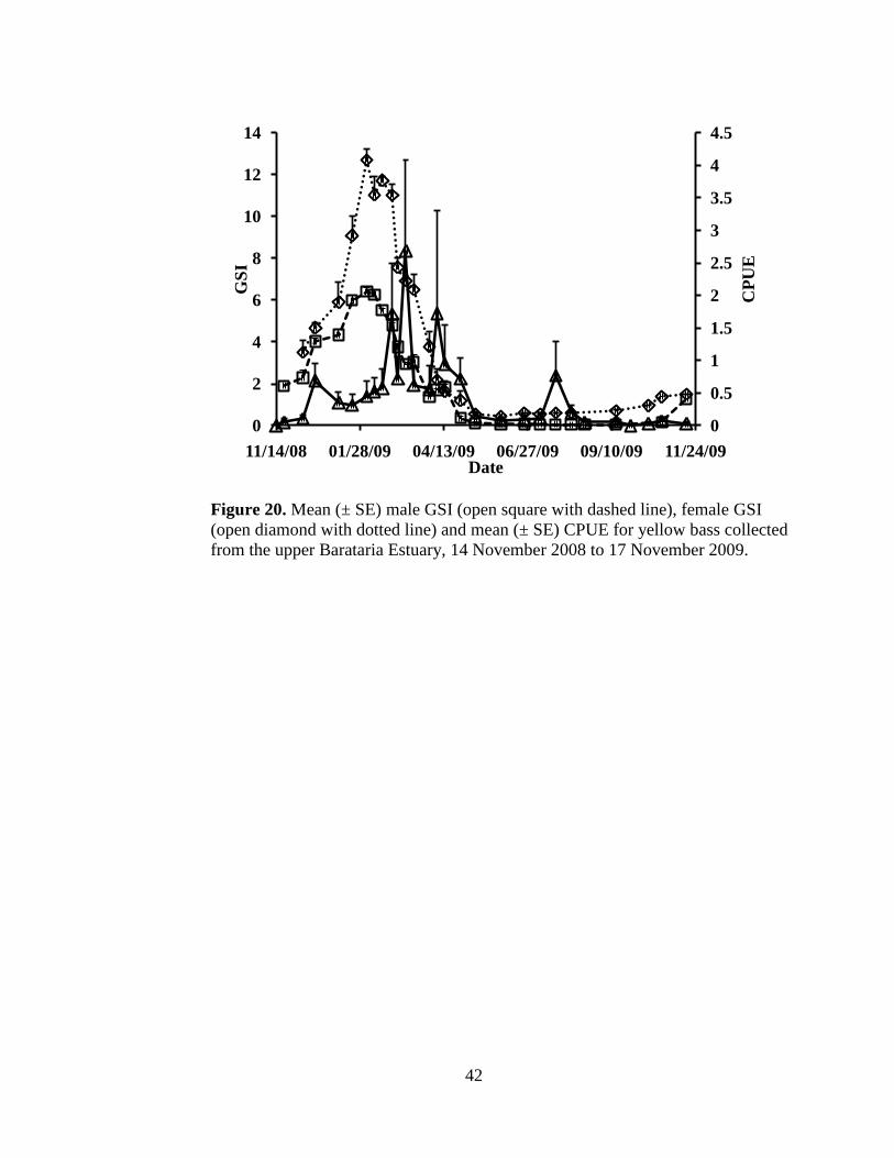
The peak in GSI occurred right before the largest peak in abundance (Figure 20).

Individual male GSI ranged from 0.03 to 7.87% (Appendix III) with an average of

2.88 ± 1.90%. Individual female GSI ranged from 0.39 to 16.74% (Appendix III)

and averaged 5.70 ± 4.34%. There was no difference in male GSI by month;

however female GSI was highest from January through March (Figure 21).

A total of 200 yellow bass (100 male and 100 female) gonads collected

from December through July were examined using histology. No “immature”

males or females were identified. Although the only 1 year old male collected

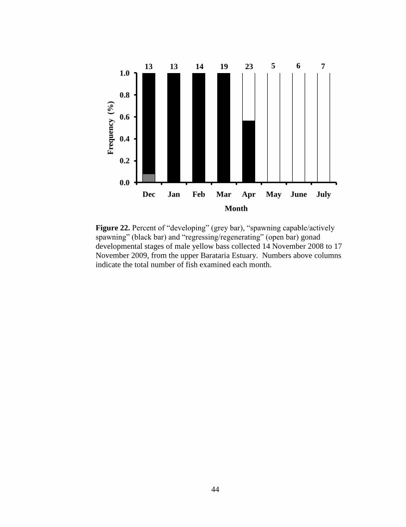
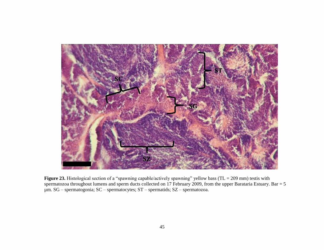
was not examined histologically. The majority of males (N = 71) were classified

as “spawning capable/actively spawning” (Figure 23) and were collected from

December through April (Figure 22). Ten males were classified as “regressing”

(Figure 24) and eighteen were classified as “regenerating” (Figure 25) and were

collected from April through July (Figure 22). Only one male, collected in

December (Figure 22), was classified as “developing” (Figure 26). Similar to

males, most of females were classified as “spawning capable” (N = 34) or

“actively spawning” (N = 25). “Spawning capable” females (Figure 28) were

collected December through April (Figure 27). Most of the “actively spawning”

females (Figure 29) were collected February through April; however one

40

Figure 18. Mean (± SE) total length at age for male (□) and female (◊) yellow

bass collected from the upper Barataria Estuary, 14 November 2008 to 17

November 2009.

0

50

100

150

200

250

300

0 1 2 3 4

Tota

l L

ength

(m

m)

Age (years)

41

Figure 19. Mean (± SE) GSI for male (solid line) and female (dashed line) yellow

bass collected from the upper Barataria Estuary, 14 November 2008 to 17

November 2009.

0

2

4

6

8

10

12

14

11/14/08 01/28/09 04/13/09 06/27/09 09/10/09 11/24/09

GS

I

Date

42

Figure 20. Mean (± SE) male GSI (open square with dashed line), female GSI

(open diamond with dotted line) and mean (± SE) CPUE for yellow bass collected

from the upper Barataria Estuary, 14 November 2008 to 17 November 2009.

0

0.5

1

1.5

2

2.5

3

3.5

4

4.5

0

2

4

6

8

10

12

14

11/14/08 01/28/09 04/13/09 06/27/09 09/10/09 11/24/09

CP

UE

GS

I

Date

43

Figure 21. Mean (± SE) monthly female yellow bass GSI. Means marked with a

similar letter are not different.

C C CC

C

AB

A

B

C

C C C

0

2

4

6

8

10

12

14

Aug Sep Oct Nov Dec Jan Feb Mar Apr May Jun Jul

Fem

ale

GS

I

Month

44


spawning” (black bar) and “regressing/regenerating” (open bar) gonad

developmental stages of male yellow bass collected 14 November 2008 to 17

November 2009, from the upper Barataria Estuary. Numbers above columns

indicate the total number of fish examined each month.

0.0

0.2

0.4

0.6

0.8

1.0

Dec Jan Feb Mar Apr May June July

Fre

qu

ency

(%

)

Month

14 19 23 5 6 71313

45

Figure 23. Histological section of a “spawning capable/actively spawning” yellow bass (TL = 209 mm) testis with

spermatozoa throughout lumens and sperm ducts collected on 17 February 2009, from the upper Barataria Estuary. Bar = 5

µm. SG – spermatogonia; SC – spermatocytes; ST – spermatids; SZ – spermatozoa.

46

Figure 24. Histological section of a “regressing” yellow bass (TL = 205 mm) testis with germinal epithelia and spermatogonia

proliferation at the periphery of testis collected 15 April 2009, in the upper Barataria Estuary. Bar = 5 µm. GE – germinal

epithelia; SG – spermatogonia; SZ – spermatozoa.

47

Figure 25. Histological section of a “regenerating” yellow bass (TL = 200) testis with empty lumens and spermatogonia

throughout collected 03 June 2009, from the upper Barataria Estuary. Bar = 5 µm. SG – spermatogonia.

48

Figure 26. Histological section of a “developing” yellow bass (TL = 195 mm) testis with spermatogonia proliferation in

spermatocysts at the periphery of the testis collected 08 December 2008, from the upper Barataria Estuary. Bar = 5µm. SG –

spermatogonia; CY – spermatocyst; SC – spermatocytes; SZ – spermatozoa.

49


spawning” (black bar) and “regressing/regenerating” (open bar) gonad

developmental stages of female yellow bass collected 14 November 2008 to 17

November 2009, from the upper Barataria Estuary. Numbers above columns

indicate the total number of fish examined each month.

0.0

0.2

0.4

0.6

0.8

1.0

Dec Jan Feb Mar Apr May June July

Fre

qu

ency

(%

)

Month

14 14 20 19 4 5 1014

50

Figure 28. Histological section of a “spawning capable” yellow bass (TL = 218 mm) ovary with a >24 hour post-ovulatory

follicle complex (Brown-Peterson et al. 2007) collected 04 March 2009, from the upper Barataria Estuary. Bar = 10 µm. PG –

primary growth oocyte; Vtg1 – primary vitellogenic oocyte; Vtg2 – secondary vitellogenic oocyte; Vtg3 – tertiary vitellogenic

oocyte; POC – post-ovulatory follicle complex.

51

Figure 29. Histological section of an “actively spawning” yellow bass (TL = 235 mm) ovary with oocytes undergoing lipid

coalescence and germinal vesicle migration collected on 10 Apr 2009, from the upper Barataria Estuary. Bar = 10 µm. PG –

primary growth oocyte; Vtg1 – primary vitellogenic oocyte; GVM – germinal vesicle migration; LC – lipid coalescence; POC

– post-ovulatory follicle complex.

52

“actively spawning” female was collected in January and in June (Figure 27).

Twelve females, collected from January through May (Figure 27), were classified

as “regressing,” (Figure 30) and twenty-one females, collected from April through

July (Figure 27), were classified as “regenerating” (Figure 31). “Developing”

(Figure 32) females were collected in December (N = 7) and February (N = 1;

Figure 27).

53

Figure 30. Histological section of a “regressing” yellow bass (TL = 230 mm) ovary with mostly atretic oocytes collected on 18

March 2009, from the upper Barataria Estuary. Bar = 10 µm. PG – primary growth oocytes; FMO – final maturation oocytes;

A – atretic oocytes.

54

Figure 31. Histological section of a “regenerating” yellow bass (TL = 225 mm) ovary collected 15 April 2009, from the upper

Barataria Estuary. Bar = 10 µm. PG – primary growth oocytes; A – atretic oocytes; OW – ovarian wall.

55

Figure 32. Histological section of a “developing” yellow bass (TL = 195 mm) ovary with many primary growth oocytes and

primary vitellogenic oocytes present throughout, collected 19 December 2009, from the upper Barataria Estuary. Bar = 10 µm.

PG – primary growth oocytes; CA – cortical alveolar oocytes; Vtg1 – primary vitellogenic oocytes; Vtg2 – secondary

vitellogenic oocytes.

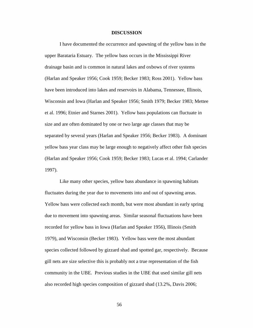
56

DISCUSSION

I have documented the occurrence and spawning of the yellow bass in the

upper Barataria Estuary. The yellow bass occurs in the Mississippi River

drainage basin and is common in natural lakes and oxbows of river systems

(Harlan and Speaker 1956; Cook 1959; Becker 1983; Ross 2001). Yellow bass

have been introduced into lakes and reservoirs in Alabama, Tennessee, Illinois,

Wisconsin and Iowa (Harlan and Speaker 1956; Smith 1979; Becker 1983; Mettee

et al. 1996; Etnier and Starnes 2001). Yellow bass populations can fluctuate in

size and are often dominated by one or two large age classes that may be

separated by several years (Harlan and Speaker 1956; Becker 1983). A dominant

yellow bass year class may be large enough to negatively affect other fish species

(Harlan and Speaker 1956; Cook 1959; Becker 1983; Lucas et al. 1994; Carlander

1997).

Like many other species, yellow bass abundance in spawning habitats

fluctuates during the year due to movements into and out of spawning areas.

Yellow bass were collected each month, but were most abundant in early spring

due to movement into spawning areas. Similar seasonal fluctuations have been

recorded for yellow bass in Iowa (Harlan and Speaker 1956), Illinois (Smith

1979), and Wisconsin (Becker 1983). Yellow bass were the most abundant

species collected followed by gizzard shad and spotted gar, respectively. Because

gill nets are size selective this is probably not a true representation of the fish

community in the UBE. Previous studies in the UBE that used similar gill nets

also recorded high species composition of gizzard shad (13.2%, Davis 2006;

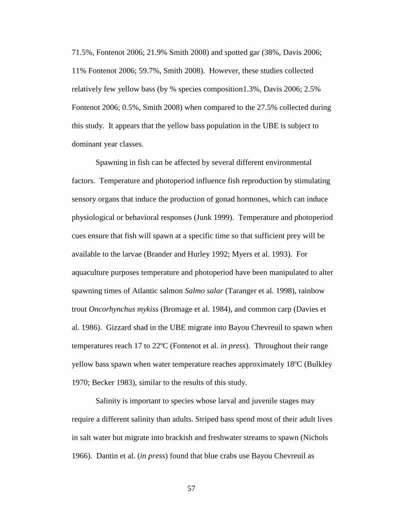
57

71.5%, Fontenot 2006; 21.9% Smith 2008) and spotted gar (38%, Davis 2006;

11% Fontenot 2006; 59.7%, Smith 2008). However, these studies collected

relatively few yellow bass (by % species composition1.3%, Davis 2006; 2.5%

Fontenot 2006; 0.5%, Smith 2008) when compared to the 27.5% collected during

this study. It appears that the yellow bass population in the UBE is subject to

dominant year classes.

Spawning in fish can be affected by several different environmental

factors. Temperature and photoperiod influence fish reproduction by stimulating

sensory organs that induce the production of gonad hormones, which can induce

physiological or behavioral responses (Junk 1999). Temperature and photoperiod

cues ensure that fish will spawn at a specific time so that sufficient prey will be

available to the larvae (Brander and Hurley 1992; Myers et al. 1993). For

aquaculture purposes temperature and photoperiod have been manipulated to alter

spawning times of Atlantic salmon Salmo salar (Taranger et al. 1998), rainbow

trout Oncorhynchus mykiss (Bromage et al. 1984), and common carp (Davies et

al. 1986). Gizzard shad in the UBE migrate into Bayou Chevreuil to spawn when

temperatures reach 17 to 22ºC (Fontenot et al. in press). Throughout their range

yellow bass spawn when water temperature reaches approximately 18ºC (Bulkley

1970; Becker 1983), similar to the results of this study.

Salinity is important to species whose larval and juvenile stages may

require a different salinity than adults. Striped bass spend most of their adult lives

in salt water but migrate into brackish and freshwater streams to spawn (Nichols

1966). Dantin et al. (in press) found that blue crabs use Bayou Chevreuil as

58

nursery and maturation grounds before migrating to coastal saline waters to

spawn. My sample sites are part of an estuary continuum that extends from the

upper reaches of Bayou Chevreuil through Lac des Allemands, Lake Salvador,

and Barataria Bay, to the Gulf of Mexico. Although salinity was representative of

a fresh water system, salt water species were collected at some of my sampling

sites. There is a possibility that under specific conditions transient peaks in

salinity could extend into the bayous of the upper Barataria Estuary, as well as a

gradual increase in ambient salinity. The effects of high salinities on the

spawning activities of yellow bass have not been documented, but it would be

likely to reduce acceptable yellow bass spawning habitat. Although yellow bass

were not sampled in saline areas of the Barataria Estuary, spawning yellow bass

were collected from fresh water regions of the estuary. Like other Moronids,

yellow bass require fresh water for spawning habitat. If salt water intrusion

continues to encroach the upper reaches of the Barataria Estuary, the area of

acceptable yellow bass spawning habitat will be reduced.

The annual flood pulse of large rivers can also be an important spawning

cue for species that rely on inundated floodplains for spawning or nursery habitat

(Junk et al. 1989). The UBE no longer receives an annual flood pulse from the

Mississippi River due to the construction of flood protection levees. The absence

of a predictable annual spring flood pulse may negatively affect the spawning of

many riverine species (Bayley 1995). Davis (2006) found that bowfin spawning

in the UBE was negatively affected by the lack of a flood pulse; however, gizzard

shad spawning did not appear to be negatively impacted (Jackson 2009; Fontenot

59

et al. in press). Because there was no flood pulse associated with yellow bass

spawning activity, it appears that the lack of a flood pulse did not negatively

impact their spawning activity. However, long term effects of no flood pulse on

yellow bass reproduction were not evaluated in this study.

Yellow bass abundance in the UBE appears to be related to spawning

activity and not water quality. Neither hypoxic (DO < 2.0 mg/L) nor brackish

(10-18 ppt) conditions were recorded during this study; however, it is unknown if

hypoxic conditions would have affected yellow bass abundance. The floodplain

did become inundated a few times during this study, but there were no changes in

yellow bass abundance in relation to water level. The photoperiod associated

with yellow bass spawning varies throughout the species’ range with spawning

occurring at shorter light periods at southern latitudes (Bulkley 1970; Becker

1983; Etnier and Starnes 2001). Yellow bass abundance increased as temperature

reached 18-22ºC, which coincides with their spawning temperatures in other parts

of their range (Bulkley 1970; Becker 1983). Therefore, yellow bass spawning

activity appears to be more strongly affected by temperature than photoperiod.

Fish of the same species may grow and mature at different rates depending

on local environmental conditions. For example, length at age of white bass in

Texas was affected by latitude and longitude, total dissolved solids, water

temperature and length of growing season (Wilde and Muoneke 2001). Gizzard

shad collected in Missouri (Michaletz 1994) were smaller than gizzard shad

collected in Alabama (Clayton and Maceina 2002) and Louisiana (Fontenot et al.

in press). Burgess (1978) reported the maximum size of yellow bass to be 275

60

mm, but Priegel (1975) reported yellow bass in Lake Poygon, Wisconsin to reach

300 mm. Yellow bass collected in this study ranged from 175 – 264 mm with the

majority (81%) between 195 and 225 mm, which is similar to the size range

reported for yellow bass in Clear Lake, Iowa (Bulkley 1970) and Lake Poygon,

Wisconsin (Priegel 1975). Yellow bass typically form size-based schools

(Burnham 1909; Ross 2001), which suggests that schooling yellow bass are the

same year class. Because the majority of yellow bass collected during this study

were within a 30 mm size range, it is likely that the yellow bass were members of

a dominant year class.

The lifespan of yellow bass is approximately six years (Lee et al. 1980;

Becker 1983; Pflieger 1997); however, maximum age varies throughout their

range. In Reelfoot Lake, Tennessee the maximum yellow bass age was 5

(Schoffman 1958), and maximum age of yellow bass in Clear Lake, Iowa was 8

years (Carlander 1997). The maximum age for yellow bass in this study was 4

years, but the majority were age 2. Females were larger than males at ages 2 and

4. This is typical for many fishes such as bowfin (Davis 2006), gizzard shad

(Fontenot et al. in press), striped bass (Nichols 1966), red drum (Turner et al.

2002), American eel Anguilla anguilla (Poole and Reynolds 1995), and scalloped

hammerhead sharks Sphyrna lewini (Klimley 1987). Because larger females have

larger ovaries and larger energy reserves when compared to smaller females,

larger females may produce more and larger eggs than smaller individuals

(Bagenal 1978; Moyle and Cech 1982).

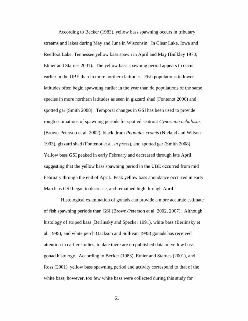
61

According to Becker (1983), yellow bass spawning occurs in tributary

streams and lakes during May and June in Wisconsin. In Clear Lake, Iowa and

Reelfoot Lake, Tennessee yellow bass spawn in April and May (Bulkley 1970;

Etnier and Starnes 2001). The yellow bass spawning period appears to occur

earlier in the UBE than in more northern latitudes. Fish populations in lower

latitudes often begin spawning earlier in the year than do populations of the same

species in more northern latitudes as seen in gizzard shad (Fontenot 2006) and

spotted gar (Smith 2008). Temporal changes in GSI has been used to provide

rough estimations of spawning periods for spotted seatrout Cynoscion nebulosus

(Brown-Peterson et al. 2002), black drum Pogonias cromis (Nieland and Wilson

1993), gizzard shad (Fontenot et al. in press), and spotted gar (Smith 2008).

Yellow bass GSI peaked in early February and decreased through late April

suggesting that the yellow bass spawning period in the UBE occurred from mid

February through the end of April. Peak yellow bass abundance occurred in early

March as GSI began to decrease, and remained high through April.

Histological examination of gonads can provide a more accurate estimate

of fish spawning periods than GSI (Brown-Peterson et al. 2002, 2007). Although

histology of striped bass (Berlinsky and Specker 1991), white bass (Berlinsky et

al. 1995), and white perch (Jackson and Sullivan 1995) gonads has received

attention in earlier studies, to date there are no published data on yellow bass

gonad histology. According to Becker (1983), Etnier and Starnes (2001), and

Ross (2001), yellow bass spawning period and activity correspond to that of the

white bass; however, too few white bass were collected during this study for

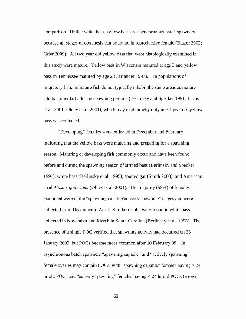
62

comparison. Unlike white bass, yellow bass are asynchronous batch spawners

because all stages of oogenesis can be found in reproductive female (Blazer 2002;

Grier 2009). All two year old yellow bass that were histologically examined in

this study were mature. Yellow bass in Wisconsin matured at age 3 and yellow

bass in Tennessee matured by age 2 (Carlander 1997). In populations of

migratory fish, immature fish do not typically inhabit the same areas as mature

adults particularly during spawning periods (Berlinsky and Specker 1991; Lucas

et al. 2001; Olney et al. 2001), which may explain why only one 1 year old yellow

bass was collected.

“Developing” females were collected in December and February

indicating that the yellow bass were maturing and preparing for a spawning

season. Maturing or developing fish commonly occur and have been found

before and during the spawning season of striped bass (Berlinsky and Specker

1991), white bass (Berlinsky et al. 1995), spotted gar (Smith 2008), and American

shad Alosa sapidissima (Olney et al. 2001). The majority (58%) of females

examined were in the “spawning capable/actively spawning” stages and were

collected from December to April. Similar results were found in white bass

collected in November and March in South Carolina (Berlinsky et al. 1995). The

presence of a single POC verified that spawning activity had occurred on 23

January 2009, but POCs became more common after 10 February 09. In

asynchronous batch spawners “spawning capable” and “actively spawning”

female ovaries may contain POCs, with “spawning capable” females having > 24

hr old POCs and “actively spawning” females having < 24 hr old POCs (Brown-

63

Peterson et al. 2007). Beginning in April, “regressing” and “regenerating”

females made up 50% of the ovaries examined and the percentage of females in

these stages continued to increase through May, June, and July. The observance

of the “regressing” and “regenerating” stages indicated that females finished

spawning and were preparing for the next spawning season. During the

“regressing” stage females undergo atresia to reabsorb remaining eggs and begin

generating primary growth oocytes in the “regenerating” stage (Brown-Peterson

et al. 2007). These data, in combination with GSI values, indicate that yellow

bass spawning occurred mid February through the end of April.

Histological analysis of gonads is more commonly applied to females

rather than males (Berlinsky and Specker 1991; Nieland and Wilson 1993;

Berlinsky et al. 1995; Brown-Peterson et al. 2002). As with the females, the

majority of the male yellow bass gonads were staged as “spawning

capable/actively spawning,” and all were collected from December through April.

Beginning in April, male yellow bass entered the “regressing” and “regenerating”

stages indicating they had finished spawning and were preparing for the next

spawning season. The occurrence of these stages suggests that male yellow bass

are not capable of spawning year round. In combination with GSI values, these

data complement female histology data that yellow bass spawning occurred from

February through the end of April.

In summary, yellow bass in the UBE follow a seasonal migration pattern

that appears to be influenced by increasing water temperatures rather than a

seasonal flood pulse. Yellow bass abundance does not appear to be related to

64

other water quality parameters; however, it is unknown how low dissolved

oxygen levels would have affected yellow bass abundance. Yellow bass were

most abundant in the UBE from February 2009 through April 2009, suggesting a

spawning aggregation. The yellow bass population in the upper Barataria Estuary

was dominated by one strong year class (age 2). Female yellow bass were larger

than male yellow bass at ages 2 and 4. GSI values indicated that yellow bass

spawned in Bayou Chevreuil from mid February through late April when water

temperatures were approximately 18-22ºC. The presence of POCs in ovaries

indicated that yellow bass spawned in early spring in the upper Barataria Estuary.

This study provides basic life history information about a lesser known species of

the Mississippi River drainage basin as well as information about the general

ecology of the upper reaches of the Barataria Estuary.

65

RECOMMENDATIONS

A long term study of the population structure of yellow bass and other

fishes in the upper Barataria Estuary would provide important information on

dominant year classes of yellow bass and their effect on other fish species. I also

recommend a long term study of the water quality of the upper Barataria Estuary

and how it affects seasonally abundant species.

A multiple year study of larval fish abundance in Bayou Chevreuil would

facilitate a better understanding of which species use the area to spawn and how

the altered hydrology affects fish reproduction in the upper Barataria Estuary.

Specifically sampling should occur throughout the water column and on

floodplain, near the banks, and in the main channel.

For future yellow bass studies, I recommend sampling throughout Lac des

Allemands, and the other lakes and bayous in the upper and lower Barataria

Estuary to find where yellow bass are located during the non-spawning season. A

telemetry project would be most beneficial for yellow bass throughout the

Barataria Estuary in identifying their yearly seasonal movement patterns. I also

suggest sampling for yellow bass during both day and night to determine yellow

bass activity throughout a 24 hour period.

I also suggest further age and growth studies of the yellow bass population

in the upper Barataria Estuary. Age has not been validated for this species. Age

validation is a necessary step in providing a better understanding of most species,

therefore age validation of yellow bass would benefit future research on the

species.

66

LITERATURE CITED

Bagenal, T.B. 1978. Aspects of fish fecundity. Pages 75-101 in S.D. Gerking,

editor. Ecology of Freshwater Fish Production. Wiley, New York.

Bailey, R.M. 1951. A checklist of the fishes of Iowa, with keys for identification.

Pages 185-237 in Iowa Fish and Fishing, by James R. Harlan and Everett

B. Speaker. Iowa State Conservation Commission.

Bayley, P.B. 1995. Understanding large river-floodplain ecosystems. BioScience

45(3):153-158.

Becker, G.C. 1983. Fishes of Wisconsin. The University of Wisconsin Press,

Madison. 1052 pp.

Berlinsky, D.L., L.F. Jackson, T.I.J. Smith, and C.V. Sullivan. 1995. The annual

reproductive cycle of the white bass, Morone chrysops. Journal of the

World Aquaculture Society 26(3):252-260.

Berlinsky, D.L. and J.L. Specker. 1991. Changes in gonadal hormones during

oocyte development in the striped bass, Morone saxatilis. Fish Physiology

and Biochemistry 9(1):51-62.

Blazer, V.S. 2002. Histopathological assessment of gonadal tissue in wild fishes.

Fish Physiology and Biochemistry 26:85-101.

Boschung, H.T., Jr. and R.L. Mayden. 2004. Fishes of Alabama. Smithsonian

Books, Washington. 736 pp.

Bosworth, B.G. and G.S. Libey. 1998. Relationships among total weight, body

shape, visceral components, and fillet traits in palmetto bass (striped bass

female Morone saxatilis x white bass male M. chrysops) and paradise bass

(striped bass female M. saxatilis x yellow bass male M. mississippiensis).

Journal of the World Aquaculture Society 29(1): 40-50.

Brander, K. and P. Hurley. 1992. Distribution of early-stage cod (Gadus morhua),

haddock (Melanogrammus aeglefinus), and witch flounder

(Glyptocephalus cynoglossus) eggs on the Scotian Shelf: a reappraisal of

evidence on the coupling of cod spawning and plankton production.

Canadian Journal of Fisheries and Aquatic Sciences 49:238-251.

Braud, D.A., A.J. Lewis, and J. Sheehan. 2006. 2005 land use/land cover

classification of the Barataria Basin. Louisiana Department of

Environmental Quality.

67

Bromage, N.R., J.A.K. Elliott, J.R.C. Springate, and C. Whitehead. 1984. The

effects of constant photoperiods on the timing of spawning in the rainbow

trout. Aquaculture 43:213-223.

Brown-Peterson, N., S. Lowerre-Barbieri, B. Macewicz, F. Saborido-Rey, J.

Tomkiewicz, and D. Wyanski. 2007. An improved and simplified

terminology for reproductive classification of fishes. Joint Meeting of

Ichthyologists and Herpetologists, St. Louis, Missouri.

Brown-Peterson, N., M.S. Peterson, D.L. Nieland, M.D. Murphy, R.G. Taylor,

and J.R. Warren. 2002. Reproductive biology of female spotted seatrout,

Cynoscion nebulosus, in the Gulf of Mexico: differences among estuaries?

Environmental Biology of Fishes 63:405-415.

Bulkley, R.V. 1970. Changes in yellow bass reproduction associated with

environmental conditions. Iowa State Journal of Science 45(2):137-180.

Burgess, G.H. 1978. Ichthyomyzon castaneus (Jordan and Eigenmann), Yellow

Bass. Page 575 in D.S. Lee et al. Atlas of North American Freshwater

Fishes. N.C. State Museum of Natural History, Raleigh. 854 pp.

Burnham, C.W. 1909. Notes on the yellow bass. Transactions of the American

Fisheries Society 39:103-108.

Carlander, K.D. 1997. Handbook of Freshwater Fishery Biology Volume 3. Iowa

State University Press, Ames.

Clayton, D.L. and M.J. Maceina. 2002. Trophic state differences in population

characteristics of gizzard shad. Lake and Reservoir Management

18(2):109-117.

Cook, F.A. 1959. Freshwater Fishes in Mississippi. Mississippi Game and Fish

Commission, Jackson.

Dantin, M.D., A.M. Ferrara, and Q.C. Fontenot. In Press. Environmental factors

affecting blue crab abundance in the hydrologically altered upper

Barataria Estuary, Louisiana. Proceedings of the Annual Conference of the

Southeastern Association of Fish and Wildlife Agencies.

Darnell, R.M. 1961. Trophic spectrum of an estuarine community, based on

studies of Lake Pontchartrain, Louisiana. Ecology 42(3):553-568.

Davies, P., I. Hanyu, K. Furukawa, and M. Nomura. 1986. Effect of temperature

and photoperiod on sexual maturation and spawning of the common carp #

3: Induction of spawning by manipulating photoperiod and temperature.

Aquaculture 52(2):137-144.

68

Davis, J. 2006. Reproductive biology, life history, and population structure of a

bowfin Amia calva population in southeastern Louisiana. Master’s Thesis,

Nicholls State University, Thibodaux, Louisiana.

Douglas, N.H. 1974. Freshwater Fishes of Louisiana. Claitor’s Publishing

Division, Baton Rouge.

Driscoll, M.P. and L.E. Miranda. 1999. Diet ecology of yellow bass,

Morone mississippiensis, in an oxbow of the Mississippi River. Journal of

Freshwater Ecology 14(4):477-486.

Dyer, H. 2007. Seasonal fish assemblages of Bayou Lafourche upstream and

downstream of the Thibodaux weir. Master’s Thesis. Nicholls State

University, Thibodaux, Louisiana.

Estay, M. 2008. Assessment of water quality in the upper Barataria Estuary.

Master’s Thesis. Nicholls State University, Thibodaux, Louisiana.

Etnier, D.A. and W.C. Starnes. 2001. Fishes of Tennessee. University of

Tennessee Press, Knoxville, pgs. 392-394.

Fontenot, J.F., A.M. Ferrara, and Q.C. Fontenot. In press. Seasonal abundance,

age structure, and spawning period of gizzard shad in the hydrologically

altered upper Barataria Estuary, Louisiana. Proceedings of the Annual

Conference of the Southeastern Association of Fish and Wildlife

Agencies.

Fontenot, J.F. 2006. Seasonal abundance, GSI, and age structure of gizzard shad

Dorosoma cepedianum in the upper Barataria Estuary. Master’s Thesis.


Fontenot, Q.C., D.A. Rutherford, and W.E. Kelso. 2001. Effects of

environmental hypoxia associated with the annual flood pulse on the

distribution of larval sunfish and shad in the Atchafalaya River Basin,

Louisiana. Transactions of the American Fisheries Society 130:107-116.

Grier, H.J., M.C.U. Aranzabal, and R. Patiño. 2009. The ovary, folliculogenesis,

and oogenesis in teleosts. Pages 25-84 in Barrie G.M. Jamieson, editor,

Reproductive Biology and Phylogeny of Fishes (Agnathans and Bony

Fishes) Volume 8A. Science Publishers, Enfield, New Hampshire.

Harlan, J.R. and E. B. Speaker. 1956. Iowa Fish and Fishing. 3rd

Edition. State of

Iowa Conservation Commission, Des Moines. 377 pp.

69

Hjort, J. 1914. Fluctuations in the great fisheries of northern Europe viewed in the

light of biological research. Rapports et process-Verbaux Des Reunions,

Conseil International pour l”Exploration de la Mer 20:1-228.

Hopkins, C.S., Jr., and J.W. Day, Jr. 1980. Modeling hydrology and

eutrophication in a Louisiana swamp forest ecosystem. Environmental

Management 4(4):325-335.

Hubbs, C., R.J. Edwards, and G.P. Garret. 1991. An annotated checklist of

freshwater fishes of Texas, with key to identification of species. Texas

Journal of Science, Supplement 43(4):1-56.

Inoue, M., D. Park, D. Justic, and W.J. Wiseman, Jr. 2008. A high-resolution

integrated hydrology-hydrodynamic model of the Barataria Basin system.

Environmental Modelling and Software 23:1122-1132.

Jackson, L.F. and C.V. Sullivan. 1995. Reproduction of the white perch: the

annual gametogenic cycle. Transactions of the American Fisheries Society

124:563-577.

Jackson, S. 2009. Seasonal diversity and abundance of larval and juvenile fishes

in the upper Barataria Estuary. Master’s Thesis, Nicholls State University,

Thibodaux, Louisiana.

Jameson, E.W. 1988. Vertebrate Reproduction. John Wiley and Sons, Inc. New

York, New York.

Jennings, S., M.J. Kaiser, and J.D. Reynolds. 2001. Marine Fisheries Ecology.

Blackwell Science Ltd., Malden, Maryland. 417 pp.

Johnson, G.D. 1984. Percoidei: development and relationships, 464-498 in H.G.

Moser, W.J. Richards, D.M. Cohen, M.P. Fahay, A.W. Kendall, Jr., and

S.L. Richardson editors. Ontogeny and Systematics of Fishes. American

Society of Ichthyologists and Herpetologists, Special Publication.

Lawrence, Kansas.

Jons, G.D. and L.E. Miranda. 1997. Ovarian weight as an index of fecundity,

maturity, and spawning periodicity. Journal of Fish Biology 50:150-156.

Jordan, D.S. and C.H. Eigenmann. 1887. Notes on the specific names of certain

North American fishes. Academy of Natural Sciences of Philadelphia

Proceedings 39:295-296.

Junk, W.J. 1999. The flood pulse concept of large rivers: learning from the

tropics. Large Rivers 11(3):261-280.

70

Junk, W.J., P.B. Bayley, and R.E. Sparks. 1989. The flood pulse concept in river

floodplain systems. Pages 110-127 in D.P. Dodge, editor. Proceedings of

the International Large River Symposium. Canadian Special Publication

of Fisheries and Aquatic Sciences 106.

Killgore, K.J. and J.J. Hoover. 2001. Effects of hypoxia on fish assemblages in a

vegetated waterbody. Journal of Aquatic Plant Management 39:40-44.

Klimley, A.P. 1987. The determinants of sexual segregation in the scalloped

hammerhead shark, Sphyrna lewini. Environmental Biology of Fishes

18(1):27-40.

Kramer, D.L. 1987. Dissolved oxygen and fish behavior. Environmental Biology

of Fishes 18(2):81-92.

Lantz, K.E. 1970. An Ecological Survey of Factors Affecting Fish Production in a

Louisiana Natural Lake and River. Louisiana Wildlife and Fisheries

Commission Fisheries Bulletin No. 6.

Lee, D.S., C.R. Gilbert, C.H. Hocutt, R.E. Jenkins, D.E. McAllister, and J.R.

Stauffer, Jr. 1980. Atlas of North American Freshwater Fishes. North

Carolina State University Museum of Natural History, Raleigh, North

Carolina.

Lin, Y.P., T.R. Petrino, and R.A. Wallace. 2004. Fundulus heteroclitus

gonadotropins.5: Small scale chromatographic fractionation of pituitary

extracts into components with different steroidogenic activities using

homologous bioassays. Reproductive Biology and Endocrinology 2(1):14.

Lowerre-Barbieri, S.K., F.E. Vose, and J.A. Whittington. 2003. Catch-and-release

fishing on a spawning aggregation of common snook: does it affect

reproductive output? Transactions of the American Fisheries Society

132:940-952.

Lucas, G., W. Hubbard, and D. Riecke. 1994. Report on the fishery survey of

Eagle Lake, 1990 to 1993. Freshwater Fisheries Report #121.

Lucas, M.C., E. Baras, T.J. Thom, A. Duncan, and O. Slavik. 2001. Migration of

Freshwater Fishes. Blackwell Science Ltd. Oxford.

Mettee, M.F., P.E. O’Neil, and J.M. Pierson. 1996. Fishes of the

Alabama and the Mobile Basin. Oxmoor House, Birmingham, Alabama,

pg. 501.

71

Michaletz, P.H. 1994. Comparison of electrofishing and gill netting for sampling

gizzard shad. Proceedings of the Annual Conference of the Southeastern

Association of Fish and Wildlife Agencies 48:533-541.

Mitchill, S.L. 1814. Report in part on the fishes of New York. New York. 28 pp.

Mommsen, T.P. and P.J. Walsh. 1988. Vitellogenesis and oocyte assembly. Pages

347-406 in W.S. Hoar and D.J. Randall, editors. Fish Physiology Volume

11, part B. Academic Press, New York.

Moyl, P.B. and J.J. Cech. 1982. Fishes: An introduction to ichthyology. Prentice-

Hall, Inc. Englewood Cliffs, New Jersey.

Myers, R.A., G. Mertz, and C.A. Bishop. 1993. Cod spawning in relation to

physical and biological cycles of the northern North-west Atlantic.

Fisheries Oceanography 2(3-4):154-165.

Nichols, P.R. 1966. The striped bass. United States Department of Interior Fish

and Wildlife Service Fishery Leaflet 592.

Nieland, D.L. and C.A. Wilson. 1993. Reproductive biology and annual variation

of reproductive variables of black drum in the northern Gulf of Mexico.

Transactions of the American Fisheries Society 122:318-327.

Olney, J.E., S.C. Denny, and J.M. Hoenig. 2001. Criteria for determining maturity

stage in female American shad, Alosa sapidissima, and a proposed

reproductive cycle. Bulletin Francais de la Pêche et de la Pisciculture 362-

363:881-901.

Page, Lawrence M., and Brooks M Burr. 1991. Freshwater Fishes: A Field Guide

to Freshwater Fishes. Houghton Mifflin Company, Boston, Massachusetts,

pg. 255.

Patiño, R. and C.V. Sullivan. 2002. Ovarian follicle growth, maturation, and

ovulation in teleost fish. Fish Physiology and Biochemistry 26:57-70.

Pflieger, W.L. 1997. The Fishes of Missouri. Missouri Department of

Conservation, Jefferson City. 372 pp.

Poole,W.R. and J.D. Reynolds. 1996. Growth rate and age at migration of

Anguilla anguilla. Journal of Fish Biology 48:633-642.

Priegel, G.R. 1975. Age and growth of the yellow bass in Lake Poygon,

Wisconsin. Transactions of the American Fisheries Society 104(3):513-

515.

72

Ross, S.T. 2001. The Inland Fishes of Mississippi. University Press of

Mississippi, Singapore. 624 pp.

Schoffman, R.J. 1958. Age and rate of growth of the yellow bass in Reelfoot

Lake, Tennessee for 1955 and 1957. Journal of the Tennessee Academy of

Science 33(1):101-105.

Secor, D.H., T.M. Trice, and H.T. Hornick. 1995. Validation of otolith-based

ageing and a comparison of otolith and scale-based ageing in mark-

recaptured Chesapeake Bay striped bass, Morone saxatilis. Fishery

Bulletin 93:186-190.

Sklar, F.H. and W.H. Conner. 1979. Effects of altered hydrology on primary

production and aquatic animal populations in a Louisiana swamp forest.

Pages 191-208 in J.W. Day, D.D. Culley, Jr., R.E. Turner, and A.J.

Mumphrey, Jr., editors. Proceedings of the Third Coastal Marsh and

Estuary Management Symposium, Louisiana Division of Continuing

Education, Baton Rouge, Louisiana.

Smith, O. 2008. Reproductive potential and life history of spotted gar Lepisosteus

oculatus in the upper Barataria Estuary, Louisiana. Master’s Thesis.


Smith, P.W. 1979. Fishes of Illinois. University of Illinois Press, Chicago. 314 pp.

Soupir, C.A., B.B. Blackwell, and M.L. Brown. 1997. Relative precision among

calcified structures for white bass age and growth assessment. Journal of

Freshwater Ecology 12(4):531-538.

Specker, J.L. and C.V. Sullivan. 1994. Vitellogenesis in fishes: status and

perspectives. Pages 304-315 in K.G. Davey, R.E. Peter, and S.S. Tobe,

editors. Perspectives in Endocrinology. National Research Council,

Ottowa, Canada.

Suthers, I.M. and J.H. Gee. 1986. Role of hypoxia in limiting diel spring and

summer distribution of juvenile yellow perch (Perca flavescens) in a

prairie marsh. Canadian Journal of Fisheries and Aquatic Sciences

43:1562-1570.

Taranger, G.L., C. Haux, S. O. Stefansson, B.T. Björnsson, B.T Walther, and T.

Hansen. 1998. Abrupt changes in photoperiod affect age at maturity,

timing of ovulation, and plasma testosterone and oestradiol-17β profile in

Atlantic salmon, Salmo salar. Aquaculture 162:85-98.

73

Turner, T.F., J.P. Wares, and J.R. Gold. 2002. Genetic effective size is three

orders of magnitude smaller than adult census size in abundant, estuarine-

dependent marine fish (Sciaenops ocellatus). Genetics 162:1329-1339.

Van Den Avyle, M.J., B.J. Higginbotham, B.T. James, and F.J. Bulow. 1983.

Habitat preferences and food habits of young-of-the-year striped bass,

white bass, and yellow bass in Watts Bar Reservoir, Tennessee. North

American Journal of Fisheries Management 3:163-170.

Welch, T.J., M.J. Van Den Avyle, R.K. Betsill and E.M. Driebe. 1993. Precision

and relative accuracy of striped bass age estimates from otoliths, scales,

and anal fin rays and spines. North American Journal of Fisheries

Management 13:616-620.

Whitehead, P.J.P. and A.C. Wheeler. 1966. The generic names used for the sea

basses of Europe and N. America (Pisces; Serranidae). Annali del Museo

Civico di Storia Naturale Giacomo Doria 76:23-41.

Wolters, W.R. and R. DeMay. 1996. Production characteristics of striped bass x

white bass and striped bass x yellow bass hybrids. Journal of the World

Aquaculture Society 27(2):202-207.

74

APPENDIX I

Appendix I. Collection date (day month year), sampling site and yellow bass

CPUE (± SE) for all dates sampled in the upper Barataria Estuary, 14 November

2008 to 17 November 2009.

Date Site CPUE ± SE

14 Nov 2008 1 0

14 Nov 2008 2 0

14 Nov 2008 3 0

21 Nov 2008 1 0.2459 ± 0.2459

21 Nov 2008 2 0

21 Nov 2008 3 0

21 Nov 2008 4 0

21 Nov 2008 5 0

21 Nov 2008 6 0

08 Dec 2008 1 0.0731 ± 0.0731

08 Dec 2008 2 0.2704 ± 0.1569

08 Dec 2008 3 0.0738 ± 0.0738

08 Dec 2008 4 0

08 Dec 2008 5 0

08 Dec 2008 6 0.0701 ± 0.0701

19 Dec 2008 1 0.3171 ± 0.2221

19 Dec 2008 2 0.7206 ± 0.4468

19 Dec 2008 3 1.2528 ± 0.6724

19 Dec 2008 4 0

19 Dec 2008 5 0.8088 ± 0.3253

19 Dec 2008 6 0

9 Jan 2009 1 0.6811 ± 0.4286

09 Jan 2009 2 0.5379 ± 0.2484

09 Jan 2009 3 0.3648 ± 0.1832

09 Jan 2009 4 0

09 Jan 2009 5 0

09 Jan 2009 6 0

21 Jan 2009 1 0.219 ± 0.219

21 Jan 2009 2 0

21 Jan 2009 3 0.1818 ± 0.1818

21 Jan 2009 4 0

21 Jan 2009 5 0.1524 ± 0.0881

21 Jan 2009 6 0.8526 ± 0.7391

03 Feb 2009 1 0.1604 ± 0.1604

03 Feb 2009 2 0.0777 ± 0.07772

03 Feb 2009 3 0.0708 ± 0.0708

03 Feb 2009 4 0

03 Feb 2009 5 1.0696 ± 0.7923

03 Feb 2009 6 0.6433 ± 0.4286

10 Feb 2009 1 0.2308 ± 0.2308

75


10 Feb 2009 2 0.2963 ± 0.2111

10 Feb 2009 3 0.0682 ± 0.0682

10 Feb 2009 4 0.2103 ± 0.2103

10 Feb 2009 5 0.3347 ± 0.1934

10 Feb 2009 6 1.19 ± 0.7446

17 Feb 2009 4 0.5652 ± 0.3266

17 Feb 2009 5 0

17 Feb 2009 6 0.7331 ± 0.4566

26 Feb 2009 1 1.2522 ± 0.8749

26 Feb 2009 2 0.2184 ± 0.2184

26 Feb 2009 3 0.4807 ± 0.2281

26 Feb 2009 4 0.149 ± 0.0861

26 Feb 2009 5 1.6351 ± 0.9878

26 Feb 2009 6 3.9777 ± 2.144

03 Mar 2009 1 1.7387 ± 0.6432

03 Mar 2009 2 0.5671 ± 0.307

03 Mar 2009 3 0.418 ± 0.1603

03 Mar 2009 4 0

03 Mar 2009 5 0.1957 ± 0.1957

03 Mar 2009 6 0.3042 ± 0.1791

10 Mar 2009 1 7.0788 ± 2.5196

10 Mar 2009 2 2.1225 ± 1.099

10 Mar 2009 3 1.0055 ± 0.4604

10 Mar 2009 4 0.9673 ± 0.6899

10 Mar 2009 5 0.6566 ± 0.3663

10 Mar 2009 6 0.2499 ± 0.0974

17 Mar 2009 1 1.3889 ± 0.665

17 Mar 2009 2 0.7799 ± 0.3568

17 Mar 2009 3 0.5359 ± 0.2661

17 Mar 2009 4 0.0664 ± 0.0664

17 Mar 2009 5 0

17 Mar 2009 6 0

31 Mar 2009 1 1.6696 ± 0.8985

31 Mar 2009 2 0.7065 ± 0.3628

31 Mar 2009 3 0

31 Mar 2009 4 0.0711 ± 0.0711

31 Mar 2009 5 0

31 Mar 2009 6 0.0636 ± 0.0636

07 Apr 2009 1 7.2106 ± 2.4068

07 Apr 2009 2 0.4813 ± 0.4813

07 Apr 2009 3 0.0411 ± 0.0411

07 Apr 2009 4 0

07 Apr 2009 5 0

07 Apr 2009 6 0

14 Apr 2009 1 2.8527 ± 1.1566

76


14 Apr 2009 2 0.758 ± 0.4509

14 Apr 2009 3 0.5441 ± 0.3304

14 Apr 2009 4 0.0798 ± 0.0798

14 Apr 2009 5 0

14 Apr 2009 6 0

28 Apr 2009 1 1.719 ± 0.7435

28 Apr 2009 2 0.0974 ± 0.0974

28 Apr 2009 3 0.2675 ± 0.1732

28 Apr 2009 4 0.2479 ± 0.2479

28 Apr 2009 5 0.283 ± 0.1634

28 Apr 2009 6 0.6149 ± 0.2463

11 May 2009 1 0

11 May 2009 2 0.1403 ± 0.0811

11 May 2009 3 0.1872 ± 0.1189

11 May 2009 4 0.2284 ± 0.2284

11 May 2009 5 0.0685 ± 0.0685

11 May 2009 6 0

03 Jun 2009 1 0

03 Jun 2009 2 0

03 Jun 2009 3 0

03 Jun 2009 4 0.0688 ± 0.0688

03 Jun 2009 5 0.2072 ± 0.1306

03 Jun 2009 6 0.0781 ± 0.0781

24 Jun 2009 1 0

24 Jun 2009 2 0

24 Jun 2009 3 0

24 Jun 2009 4 0

24 Jun 2009 5 0.3395 ± 0.2623

24 Jun 2009 6 0.0605 ± 0.0605

08 Jul 2009 1 0.075 ± 0.075

08 Jul 2009 2 0

08 Jul 2009 3 0

08 Jul 2009 4 0.0777 ± 0.0777

08 Jul 2009 5 0.2243 ± 0.144

08 Jul 2009 6 0.137 ± 0.137

22 Jul 2009 1 0

22 Jul 2009 2 0.0714 ± 0.0714

22 Jul 2009 3 0

22 Jul 2009 4 2.361 ± 1.0886

22 Jul 2009 5 1.0268 ± 0.653

22 Jul 2009 6 0

05 Aug 2009 1 0.1721 ± 0.1025

05 Aug 2009 2 0.0638 ± 0.0638

05 Aug 2009 3 0.056 ± 0.056

05 Aug 2009 4 0

77


05 Aug 2009 5 0.5629 ± 0.1974

05 Aug 2009 6 0.0664 ± 0.0664

17 Aug 2009 1 0

17 Aug 2009 2 0

17 Aug 2009 3 0.0893 ± 0.0893

17 Aug 2009 4 0.1558 ± 0.09

17 Aug 2009 5 0

17 Aug 2009 6 0

14 Sep 2009 1 0

14 Sep 2009 2 0

14 Sep 2009 3 0

14 Sep 2009 4 0.2836 ± 0.0095

14 Sep 2009 5 0

14 Sep 2009 6 0.0607 ± 0.0607

27 Sep 2009 1 0

27 Sep 2009 2 0

27 Sep 2009 3 0

27 Sep 2009 4 0

27 Sep 2009 5 0

27 Sep 2009 6 0

13 Oct 2009 1 0.0773 ± 0.0773

13 Oct 2009 2 0

13 Oct 2009 3 0.0714 ± 0.0714

13 Oct 2009 4 0

13 Oct 2009 5 0

13 Oct 2009 6 0

25 Oct 2009 1 0

25 Oct 2009 2 0.2035 ± 0.1317

25 Oct 2009 3 0.1255 ± 0.1255

25 Oct 2009 4 0

25 Oct 2009 5 0

25 Oct 2009 6 0

17 Nov 2009 1 0

17 Nov 2009 2 0.1345 ± 0.1345

17 Nov 2009 3 0

17 Nov 2009 4 0

17 Nov 2009 5 0

17 Nov 2009 6 0

78

APPENDIX II

Appendix II. Collection date (day month year), sampling site, dissolved oxygen

(DO; mg/L), temperature (ºC), salinity (ppt), and specific conductance (µS) for all

dates sampled in the upper Barataria Estuary, 14 November 2008 to 17 November

2009. ND = no data.

Date Site DO

(mg/L)

Temperature

(°C)

Salinity

(ppt)

Specific

Conductance

(µS)

14 Nov 2008 1 9.58 20.8 0.3 658

14 Nov 2008 2 8.29 21.5 0.3 639

14 Nov 2008 3 10.06 20.9 0.2 481

14 Nov 2008 4 9.83 19.2 0.1 247.1

14 Nov 2008 5 5.78 18.4 0.1 253.3

14 Nov 2008 6 4.22 18.1 0.1 258.7

21 Nov 2008 1 7.79 13.3 0.3 438.2

21 Nov 2008 2 7.52 13.2 0.3 424.4

21 Nov 2008 3 7.65 13.2 0.3 405.1

21 Nov 2008 4 3.78 15.5 0.1 203.1

21 Nov 2008 5 3.02 14.3 0.1 206.3

21 Nov 2008 6 2.99 14.7 0.1 210.6

8 Dec 2008 1 8.5 12.6 0.3 550

8 Dec 2008 2 8.57 12.9 0.2 316.9

8 Dec 2008 3 9.62 12.7 0.2 197.6

8 Dec 2008 4 3.9 14.5 0.1 212

8 Dec 2008 5 3.74 13.5 0.1 209.6

8 Dec 2008 6 3.21 12.7 0.1 205.5

19 Dec 2008 1 7.73 16.7 0.2 376.1

19 Dec 2008 2 8.7 18.1 0.1 270.1

19 Dec 2008 3 8.64 18.9 0.1 263.7

19 Dec 2008 4 0.71 18.2 0.1 225.6

19 Dec 2008 5 0.94 19.6 0.1 208.8

19 Dec 2008 6 0.71 19.1 0.1 212.4

9 Jan 2009 1 5.28 17.5 0.1 238.8

9 Jan 2009 2 5.09 17.6 0.1 198.9

9 Jan 2009 3 6.22 17.4 0.2 276.8

9 Jan 2009 4 1.43 16.5 0.1 182.4

9 Jan 2009 5 2.26 15.8 0.1 129.8

9 Jan 2009 6 2.03 16.3 0.1 128.4

21 Jan 2009 1 9.05 11.6 0.2 273.3

21 Jan 2009 2 8.25 10.7 0.1 209.3

21 Jan 2009 3 8.16 10.4 0.1 146.7

21 Jan 2009 4 4.11 11.5 0.1 158

21 Jan 2009 5 4.7 11.1 0.1 139.3

21 Jan 2009 6 4.22 11.5 0.1 140.5

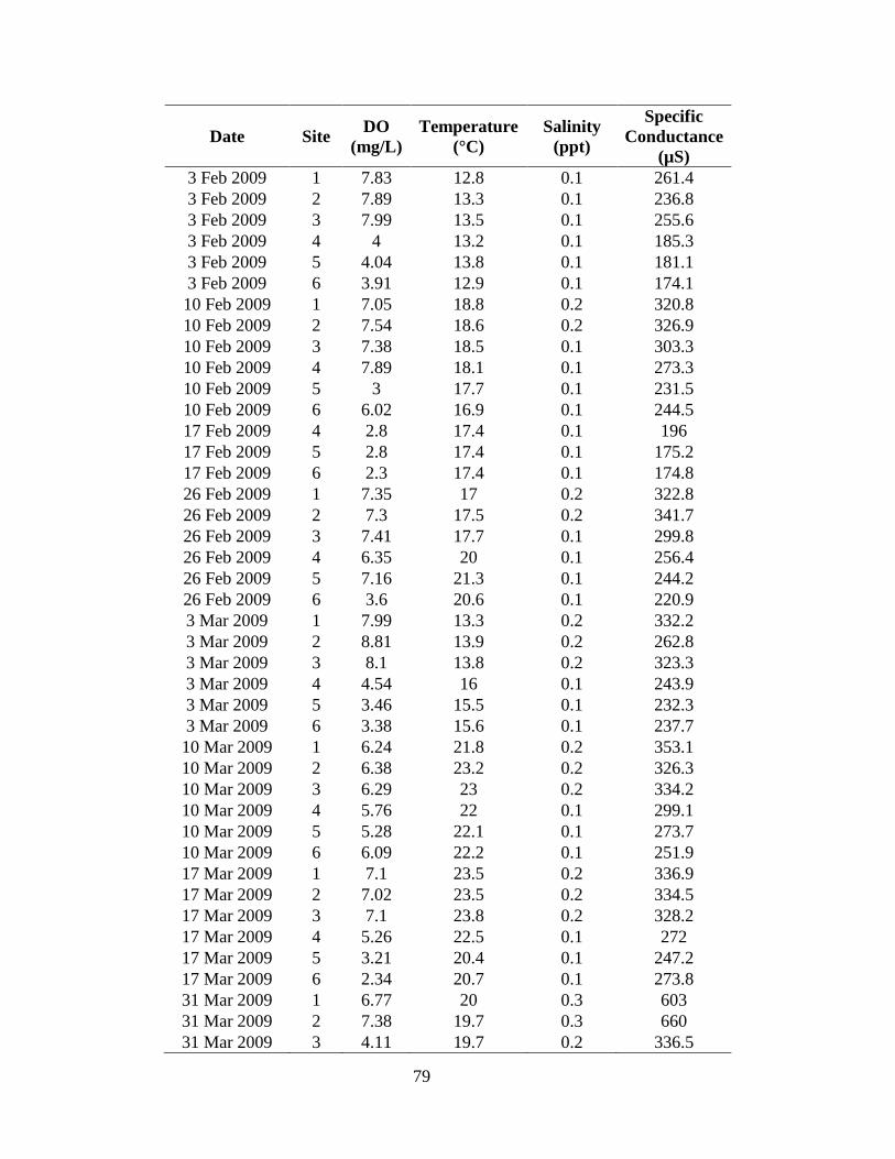
79

Date Site DO

(mg/L)

Temperature

(°C)

Salinity

(ppt)

Specific

Conductance

(µS)

3 Feb 2009 1 7.83 12.8 0.1 261.4

3 Feb 2009 2 7.89 13.3 0.1 236.8

3 Feb 2009 3 7.99 13.5 0.1 255.6

3 Feb 2009 4 4 13.2 0.1 185.3

3 Feb 2009 5 4.04 13.8 0.1 181.1

3 Feb 2009 6 3.91 12.9 0.1 174.1

10 Feb 2009 1 7.05 18.8 0.2 320.8

10 Feb 2009 2 7.54 18.6 0.2 326.9

10 Feb 2009 3 7.38 18.5 0.1 303.3

10 Feb 2009 4 7.89 18.1 0.1 273.3

10 Feb 2009 5 3 17.7 0.1 231.5

10 Feb 2009 6 6.02 16.9 0.1 244.5

17 Feb 2009 4 2.8 17.4 0.1 196

17 Feb 2009 5 2.8 17.4 0.1 175.2

17 Feb 2009 6 2.3 17.4 0.1 174.8

26 Feb 2009 1 7.35 17 0.2 322.8

26 Feb 2009 2 7.3 17.5 0.2 341.7

26 Feb 2009 3 7.41 17.7 0.1 299.8

26 Feb 2009 4 6.35 20 0.1 256.4

26 Feb 2009 5 7.16 21.3 0.1 244.2

26 Feb 2009 6 3.6 20.6 0.1 220.9

3 Mar 2009 1 7.99 13.3 0.2 332.2

3 Mar 2009 2 8.81 13.9 0.2 262.8

3 Mar 2009 3 8.1 13.8 0.2 323.3

3 Mar 2009 4 4.54 16 0.1 243.9

3 Mar 2009 5 3.46 15.5 0.1 232.3

3 Mar 2009 6 3.38 15.6 0.1 237.7

10 Mar 2009 1 6.24 21.8 0.2 353.1

10 Mar 2009 2 6.38 23.2 0.2 326.3

10 Mar 2009 3 6.29 23 0.2 334.2

10 Mar 2009 4 5.76 22 0.1 299.1

10 Mar 2009 5 5.28 22.1 0.1 273.7

10 Mar 2009 6 6.09 22.2 0.1 251.9

17 Mar 2009 1 7.1 23.5 0.2 336.9

17 Mar 2009 2 7.02 23.5 0.2 334.5

17 Mar 2009 3 7.1 23.8 0.2 328.2

17 Mar 2009 4 5.26 22.5 0.1 272

17 Mar 2009 5 3.21 20.4 0.1 247.2

17 Mar 2009 6 2.34 20.7 0.1 273.8

31 Mar 2009 1 6.77 20 0.3 603

31 Mar 2009 2 7.38 19.7 0.3 660

31 Mar 2009 3 4.11 19.7 0.2 336.5

80

Date Site DO

(mg/L)

Temperature

(°C)

Salinity

(ppt)

Specific

Conductance

(µS)

31 Mar 2009 4 1.58 20.2 0.1 245.8

31 Mar 2009 5 1.28 19.6 0.1 181.4

31 Mar 2009 6 1.4 20.3 0.1 139.6

7 Apr 2009 1 7.96 21.5 0.1 237

7 Apr 2009 2 8.61 21.5 0.2 332

7 Apr 2009 3 6.26 21.8 0.1 237

7 Apr 2009 4 ND ND ND ND



14 Apr 2009 1 7.91 21.2 0.1 296

14 Apr 2009 2 8.4 21.5 0.1 227

14 Apr 2009 3 7.5 21.8 0.1 215

14 Apr 2009 4 3.3 22.1 0.1 202

14 Apr 2009 5 2.44 21.9 0.1 186

14 Apr 2009 6 1.91 21.8 0.1 177

28 Apr 2009 1 8.53 24.6 0.3 558

28 Apr 2009 2 8.39 24.8 0.3 572

28 Apr 2009 3 8.86 25 0.2 386

28 Apr 2009 4 5.21 25.2 0.1 239

28 Apr 2009 5 7.6 25.4 0.1 324

28 Apr 2009 6 7.65 24.6 0.2 431

11May 2009 1 6.53 27.9 0.2 403

11 May 2009 2 8.87 27.4 0.2 354

11 May 2009 3 4.33 27.6 0.1 266

11 May 2009 4 1.88 27.7 0.1 183

11 May 2009 5 1.64 27.2 0.1 139

11 May 2009 6 1.22 27.2 0.1 115

3 Jun 2009 1 7.77 27.5 0.2 368

3 Jun 2009 2 8.56 27.5 0.2 311

3 Jun 2009 3 8.71 27.7 0.1 284

3 Jun 2009 4 5.1 27.5 0.1 183

3 Jun 2009 5 3.52 26.4 0.1 135

3 Jun 2009 6 3.2 25.2 0.1 126

24 Jun 2009 1 5.56 31.1 0.2 413.8

24 Jun 2009 2 4.06 30.9 0.2 387

24 Jun 2009 3 6.85 31.5 0.2 375.2

24 Jun 2009 4 3.98 33 0.1 214.2

24 Jun 2009 5 4.04 32.4 0.1 197.8

24 Jun 2009 6 5.54 33.8 0.1 207.3

8 Jul 2009 1 6.6 30.1 0.2 343.2

8 Jul 2009 2 7.9 30.2 0.2 333

8 Jul 2009 3 5.56 29.6 0.2 317.5

81

Date Site DO

(mg/L)

Temperature

(°C)

Salinity

(ppt)

Specific

Conductance

(µS)

8 Jul 2009 4 2.96 30.1 0.1 227.5

8 Jul 2009 5 3.07 29.6 0.1 267.8

8 Jul 2009 6 2.39 29.1 0.1 216.1

22 Jul 2009 1 2.8 29.1 0.2 342.3

22 Jul 2009 2 4.46 29.2 0.2 342.1

22 Jul 2009 3 4.64 29.4 0.2 316

22 Jul 2009 4 4.15 29.4 0.1 300.2

22 Jul 2009 5 4.73 29.3 0.1 303

22 Jul 2009 6 0.88 28.6 0.1 247.5

5 Aug 2009 1 3.39 31.5 0.2 ND

5 Aug 2009 2 4.32 31.6 0.2 ND

5 Aug 2009 3 4.4 31.6 0.2 ND

5 Aug 2009 4 6.21 30.5 0.1 190.1

5 Aug 2009 5 7.23 30.6 0.1 196.4

5 Aug 2009 6 7.03 30.6 0.1 217.7

17 Aug 2009 1 2.45 30.9 0.2 879.7

17 Aug 2009 2 3.55 30.9 0.2 870.5

17 Aug 2009 3 4.77 31.8 0.2 855.6

17 Aug 2009 4 3.06 32.7 0.2 ND

17 Aug 2009 5 2.4 30.6 0.1 199

17 Aug 2009 6 2.77 31.2 0.1 174.3

14 Sep 2009 1 9.07 27.8 0.1 436.1

14 Sep 2009 2 10.12 27.8 0.1 420.4

14 Sep 2009 3 7.02 27.8 0.1 413

14 Sep 2009 4 6.3 27.2 0.2 375.5

14 Sep 2009 5 2.13 27.4 0.1 186.4

14 Sep 2009 6 2.14 26.8 0.1 150.9

27 Sep 2009 1 11.13 32.3 0.2 453.5

27 Sep 2009 2 10.43 31.9 0.2 418.8

27 Sep 2009 3 10.23 31.7 0.1 270.6

27 Sep 2009 4 1.15 27.1 0.1 183.7

27 Sep 2009 5 0.84 27.1 0.1 137.1

27 Sep 2009 6 0.95 27.2 0.1 120.1

13 Oct 2009 1 11.55 26.3 0.2 362.4

13 Oct 2009 2 7.82 26.8 0.2 371.7

13 Oct 2009 3 7.14 26.5 0.1 243

13 Oct 2009 4 1.07 25.3 0.1 167.7

13 Oct 2009 5 0.7 25.2 0.1 128.1

13 Oct 2009 6 0.75 25.4 0.1 127.7

25 Oct 2009 1 14.3 19.8 0.1 216.1

25 Oct 2009 2 8.2 19.7 0.1 233.4

25 Oct 2009 3 7.78 19.9 0.1 198.1

82

Date Site DO

(mg/L)

Temperature

(°C)

Salinity

(ppt)

Specific

Conductance

(µS)

25 Oct 2009 4 3.6 19.9 0.1 627.6

25 Oct 2009 5 3.24 18.7 0.1 123.7

25 Oct 2009 6 3.67 18.7 0.1 119.9

17 Oct 2009 1 9.11 17 0.1 231.4

17 Oct 2009 2 7.53 17.5 0.1 211.9

17 Oct 2009 3 6.74 17.2 0.1 200.3

17 Oct 2009 4 ND ND ND ND



83

APPENDIX III

Appendix III. Collection date (day month year) sampling site, sex, number collected, total length (TL ± SE), total weight (Wt ± SE),

and gonadosomatic index (GSI ± SE) for yellow bass collected in the upper Barataria Estuary, 14 November 2008 to 17 November

2009.

Date Site Sex N TL ± SE Wt ± SE GSI ± SE

21 Nov 2008 1 M 1 195 106 1.9

08 Dec 2008 1 M 1 195 113.5 1.8

08 Dec 2008 2 F 2 207.5 ± 2.5 127 ± 2 3.9 ± 0.4

08 Dec 2008 2 M 2 197.5 ± 2.5 108.5 ± 0.5 2.5 ± 0.5

08 Dec 2008 3 F 1 208 131 1.9

08 Dec 2008 6 F 1 220 161 4.3

19 Dec 2008 1 F 3 214 ± 2.3 139.7 ± 1.7 3.8 ± 0.5

19 Dec 2008 1 M 1 202 128 5

19 Dec 2008 2 F 4 209.5 ± 2.5 148. ± 7.7 4.5 ± 0.2

19 Dec 2008 2 M 6 204.5 ± 2. 132.5 ± 9.1 3.8 ± 0.3

19 Dec 2008 3 F 10 211.3 ± 2.4 146.5 ± 9.2 4.4 ± 0.4

19 Dec 2008 3 M 9 205 ± 3.1 130.1 ± 5.2 3.8 ± 0.2

19 Dec 2008 5 F 10 219.6 ± 6.9 168.5 ± 16.5 5.3 ± 0.5

19 Dec 2008 5 M 6 217 ± 9.7 168.1 ± 22.5 4.3 ± 0.3

09 Jan 2009 1 F 4 208.5 ± 3.8 144.6 ± 19.1 6.1 ± 1.6

09 Jan 2009 1 M 7 202 ± 2.2 127 ± 2 4.4 ± 0.4

09 Jan 2009 2 F 5 210.4 ± 3.9 148.3 ± 15.3 5.7 ± 1.3

09 Jan 2009 2 M 3 203.7 ± 5.5 129.2 ± 7 5.1 ± 0.2

09 Jan 2009 3 M 5 199.6 ± 4.4 116.7 ± 6.2 3.8 ± 0.5

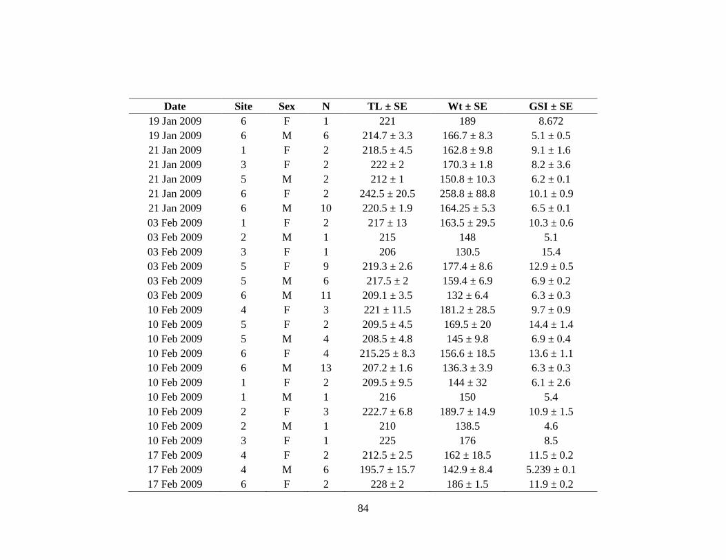
84


19 Jan 2009 6 F 1 221 189 8.672

19 Jan 2009 6 M 6 214.7 ± 3.3 166.7 ± 8.3 5.1 ± 0.5

21 Jan 2009 1 F 2 218.5 ± 4.5 162.8 ± 9.8 9.1 ± 1.6

21 Jan 2009 3 F 2 222 ± 2 170.3 ± 1.8 8.2 ± 3.6

21 Jan 2009 5 M 2 212 ± 1 150.8 ± 10.3 6.2 ± 0.1

21 Jan 2009 6 F 2 242.5 ± 20.5 258.8 ± 88.8 10.1 ± 0.9

21 Jan 2009 6 M 10 220.5 ± 1.9 164.25 ± 5.3 6.5 ± 0.1

03 Feb 2009 1 F 2 217 ± 13 163.5 ± 29.5 10.3 ± 0.6

03 Feb 2009 2 M 1 215 148 5.1

03 Feb 2009 3 F 1 206 130.5 15.4

03 Feb 2009 5 F 9 219.3 ± 2.6 177.4 ± 8.6 12.9 ± 0.5

03 Feb 2009 5 M 6 217.5 ± 2 159.4 ± 6.9 6.9 ± 0.2

03 Feb 2009 6 M 11 209.1 ± 3.5 132 ± 6.4 6.3 ± 0.3

10 Feb 2009 4 F 3 221 ± 11.5 181.2 ± 28.5 9.7 ± 0.9

10 Feb 2009 5 F 2 209.5 ± 4.5 169.5 ± 20 14.4 ± 1.4

10 Feb 2009 5 M 4 208.5 ± 4.8 145 ± 9.8 6.9 ± 0.4

10 Feb 2009 6 F 4 215.25 ± 8.3 156.6 ± 18.5 13.6 ± 1.1

10 Feb 2009 6 M 13 207.2 ± 1.6 136.3 ± 3.9 6.3 ± 0.3

10 Feb 2009 1 F 2 209.5 ± 9.5 144 ± 32 6.1 ± 2.6

10 Feb 2009 1 M 1 216 150 5.4

10 Feb 2009 2 F 3 222.7 ± 6.8 189.7 ± 14.9 10.9 ± 1.5

10 Feb 2009 2 M 1 210 138.5 4.6

10 Feb 2009 3 F 1 225 176 8.5

17 Feb 2009 4 F 2 212.5 ± 2.5 162 ± 18.5 11.5 ± 0.2

17 Feb 2009 4 M 6 195.7 ± 15.7 142.9 ± 8.4 5.239 ± 0.1

17 Feb 2009 6 F 2 228 ± 2 186 ± 1.5 11.9 ± 0.2

85


17 Feb 2009 6 M 15 210.9 ± 1.5 138.9 ± 2.8 5.6 ± 0.1

26 Feb 2009 1 F 1 215 178.5 15.6

26 Feb 2009 1 M 15 201.3 ± 2.6 121.7 ± 5.1 4.3 ± 0.3

26 Feb 2009 2 F 1 214 151 10.1

26 Feb 2009 2 M 2 208.5 ± 3.5 126 ± 13.5 4.7 ± 0.6

26 Feb 2009 3 F 4 212.5 ± 5.2 153.8 ± 6.3 9.8 ± 2.2

26 Feb 2009 3 M 3 196.7 ± 2.7 112.3 ± 10 4.7 ± 0.5

26 Feb 2009 4 M 2 212.5 ± 10.5 136 ± 12 4.7 ± 0.2

26 Feb 2009 5 F 12 214.6 ± 2.9 155.4 ± 6.1 11.7 ± 0.8

26 Feb 2009 5 M 14 209 ± 3 135.2 ± 5.4 4.8 ± 0.2

26 Feb 2009 6 F 14 214.8 ± 2.4 152.2 ± 5.8 10.5 ± 0.7

26 Feb 2009 6 M 67 213.2 ± 0.9 137.4 ± 1.9 5 ± 0.1

03 Mar 2009 1 F 1 203 123 6.9

03 Mar 2009 5 M 2 207.5 ± 2.5 124 4.1 ± 0.7

03 Mar 2009 6 M 5 208 ± 6.6 122.6 ± 11.2 4.2 ± 0.5

03 Mar 2009 1 M 23 201.6 ± 1.9 120 ± 3.5 3.7 ± 0.2

03 Mar 2009 2 F 5 210.8 ± 4.7 143.4 ± 9.6 7.3 ± 0.6

03 Mar 2009 2 M 3 213.3 ± 6.2 153.8 ± 10 4 ± 0.1

03 Mar 2009 3 F 4 203.5 ± 3.5 140.3 ± 8.4 8.1 ± 0.9

03 Mar 2009 3 M 1 209 126 2.7

10 Mar 2009 4 F 4 215.8 ± 5.1 145.4 ± 11.6 4.9 ± 0.2

10 Mar 2009 4 M 9 213.8 ± 2.6 132 ± 4.1 3.8 ± 0.2

10 Mar 2009 5 F 6 217.5 ± 4.1 150 ± 7.5 7.7 ± 1.4

10 Mar 2009 5 M 5 208.2 ± 2.8 124.8 ± 4.3 3.7 ± 0.3

10 Mar 2009 6 F 3 210.7 ± 5.4 132.3 ± 6.6 7.4 ± 0.9

10 Mar 2009 6 M 2 201.5 ± 2.5 106.8 ± 5.3 4 ± 1.43

86


10 Mar 2009 1 F 19 209.1 ± 2.6 139.8 ± 4.5 6.7 ± 0.4

10 Mar 2009 1 M 85 206.2 ± 1.5 123.4 ± 2.2 2.8 ± 0.1

10 Mar 2009 2 F 14 213.6 ± 2.4 148.3 ± 4.7 6.9 ± 0.5

10 Mar 2009 2 M 26 207.3 ± 1.9 124.9 ± 3.5 2.9 ± 0.2

10 Mar 2009 3 F 8 208.8 ± 3.7 145.9 ± 10.5 7.5 ± 0.7

10 Mar 2009 3 M 11 208.3 ± 2.3 131.5 ± 8.9 2.9 ± 0.2

17 Mar 2009 4 M 1 200 120.5 3.3

17 Mar 2009 1 F 4 211.3 ± 4.5 149.9 ± 9.1 5.8 ± 1.1

17 Mar 2009 1 M 18 208.9 ± 2.3 130.2 ± 4.5 2.6 ± 0.2

17 Mar 2009 2 F 5 211.4 ± 4.8 146.9 ± 9.7 7 ± 1.3

17 Mar 2009 2 M 6 201.7 ± 4.1 117.5 ± 6.1 4.5 ± 1.5

17 Mar 2009 3 F 4 211.3 ± 6.6 148.5 ± 12.6 6.7 ± 1.6

17 Mar 2009 3 M 3 204.7 ± 5.8 126.3 ± 10.9 2.1 ± 0.4

31 Mar 2009 4 M 1 225 166.5 1.4

31 Mar 2009 6 F 1 204 118 3

31 Mar 2009 1 F 12 211.6 ± 3 138.8 ± 6.2 4.6 ± 0.9

31 Mar 2009 1 M 14 203.4 ± 2 117.8 ± 3.2 1.2 ± 0.2

31 Mar 2009 2 F 3 211 ± 0.6 133.3 ± 3.6 0.9

31 Mar 2009 2 M 6 204 ± 1.5 121.7 ± 2.9 1.9 ± 0.3

07 Apr 2009 1 F 5 223.6 ± 3.1 161.5 ± 8.3 3.5 ± 0.6

07 Apr 2009 1 M 197 209 ± 0.7 134.6 ± 1.4 1.7± 0.1

07 Apr 2009 2 F 9 213.8 ± 3 150 ± 6.6 1.5 ± 0.7

07 Apr 2009 2 M 4 204 ± 6.1 125.1 ± 7.3 1.6 ± 0.2

07 Apr 2009 3 M 1 200 126.5 1.9

14 Apr 2009 4 M 1 215 135.5 1.4

14 Apr 2009 1 F 3 217 ± 5.7 145.3 ± 5.4 1.5 ± 0.9

87


14 Apr 2009 1 M 32 205.5 ± 1.6 125.2 ± 2.9 2 ± 0.2

14 Apr 2009 2 F 4 204.3 ± 3.6 130.1 ± 1.8 1.7 ± 0.8

14 Apr 2009 2 M 6 206.3 ± 5 123.2 ± 8.6 1.6 ± 0.4

14 Apr 2009 3 F 2 219 ± 1 151 ± 5.5 1.8 ± 1.2

14 Apr 2009 3 M 6 213.8 ± 3.1 131.2 ± 5 1.6 ± 0.4

28 Apr 2009 4 F 2 208 ± 3 135 ± 4 4.6 ± 3.9

28 Apr 2009 4 M 2 194.5 ± 19.5 126.5 ± 2.5 0.3 ± 0.2

28 Apr 2009 5 F 3 211 ± 3.2 132.8 ± 14.3 1.3 ± 0.2

28 Apr 2009 6 F 3 212 ± 6 142.3 ± 9 0.6 ± 0.1

28 Apr 2009 6 M 6 187 ± 13.5 115.8 ± 3 0.4 ± 0.2

28 Apr 2009 1 F 8 213 ± 2.1 141.5 ± 4.1 0.6 ± 0.1

28 Apr 2009 1 M 9 206.1 ± 2.6 124.4 ± 5.2 0.3 ± 0.1

28 Apr 2009 2 M 1 195 105 0.7

28 Apr 2009 3 F 1 215 147 0.5

28 Apr 2009 3 M 2 213 ± 3 148.5 ± 5.5 0.2

11 May 2009 4 F 1 217 130 0.6

11 May 2009 4 M 2 214 ± 1 143.3 ± 1.75 0.1

11 May 2009 5 M 1 216 146 0.2

11 May 2009 2 F 2 185 ± 25 148.8 ± 20.75 0.5 ± 0.1

11 May 2009 3 F 1 192 93 0.5

11 May 2009 3 M 2 209.5 ± 6.5 127 ± 19 0.1

03 Jun 2009 4 M 1 200 134.5 0.1

03 Jun 2009 5 M 3 212 141.5 ± 1.6 0.1

03 Jun 2009 6 F 1 216 155.5 0.4

24 Jun 2009 5 F 3 185.7 ± 20.8 132.3 ± 9.4 0.6

24 Jun 2009 5 M 2 175 ± 30 107.5 ± 1.5 0.1

88


24 Jun 2009 6 F 1 182 116.5 0.6

08 Jul 2009 4 F 1 211 133.5 0.4

08 Jul 2009 5 F 3 197.7 ± 13.8 152.5 ± 10.4 0.5 ± 0.1

08 Jul 2009 6 F 1 207 133 0.6

08 Jul 2009 6 M 1 170 149 0.1

08 Jul 2009 1 M 1 206 118 0.1

22 Jul 2009 4 F 12 212 ± 3 134.1 ± 4.9 0.6

22 Jul 2009 4 M 22 204.9 ± 4.3 129. ± 2.6 0.1

22 Jul 2009 5 F 10 213.1 ± 6.6 154 ± 6.3 0.6

22 Jul 2009 5 M 7 211.9 ± 4.2 144.4 ± 6.7 0.1

22 Jul 2009 2 F 1 219 149.5 0.6

05 Aug 2009 5 F 1 220 154.5 0.5

05 Aug 2009 5 M 7 212.9 ± 2 148.7 ± 2 0.1

05 Aug 2009 6 F 1 226 171 0.6

05 Aug 2009 1 F 1 228 165.5 0.7

05 Aug 2009 1 M 1 185 121.5 0.1

05 Aug 2009 2 F 1 211 137 0.7

05 Aug 2009 3 F 1 220 157 0.6

17 Aug 2009 4 M 2 215.5 ± 6.5 157.3 ± 29.8 0.1

17 Aug 2009 3 M 1 208 168.5 0.1

14 Sep 2009 4 F 2 218 147.3 ± 4.3 0.7 ± 0.1

14 Sep 2009 4 M 3 213.3 ± 2.2 144.3 ± 3.9 0.1

14 Sep 2009 6 F 1 220 168.5 0.7

13 Oct 2009 1 F 1 209 124.5 1

13 Oct 2009 3 F 1 205 119 0.9

26 Oct 2009 2 M 3 211.7 ± 3.3 137.7 ± 9.2 0.2 ± 0.1

89


26 Oct 2009 3 F 1 220 156 1.4

26 Oct 2009 3 M 1 210 118.5 0.1

17 Nov 2009 2 F 1 214 150 1.5

17 Nov 2009 2 M 1 221 157.5 1.3

90

BIOGRAPHICAL SKETCH

Cynthia Nichole Fox was born on September 4, 1984, in Crossville,

Tennessee. After graduating as Salutatorian from Hermitage Springs High School

in Hermitage Springs, Tennessee, in 2003, Cynthia attended Tennessee Tech

University. While at Tennessee Tech, Cynthia served as president of the Beta

Beta Beta Honorary Biological Society for 3 years. Cynthia graduated cum laude

from Tennessee Tech University in May of 2007 with a B.S. in Biology with a

marine science concentration. In the fall of 2007, Cynthia was awarded an

internship at Mote Marine Laboratory’s Center for Shark Research and Aquarium,

in Sarasota, Florida. During her internship at Mote, Cynthia assisted in several

research projects including the endangered Smalltooth Sawfish Management and

Outreach project. Cynthia then enrolled in the Marine and Environmental Biology

graduate program at Nicholls State University, in Thibodaux, Louisiana. Cynthia

conducted research on the life history and gonad histology of yellow bass in the

upper Barataria Estuary. While at Nicholls State, Cynthia assisted in coastal

restoration and clean-up, benthic invertebrate collection, and bird banding and

recapture projects, and interned with Bayou Land RC&D and Bois d’Arc

Gardens. After graduation in May 2010, Cynthia will either continue her

education in a Ph.D. program or pursue a career as a biologist.

91

CURRICULUM VITAE

Cynthia Nichole Fox

Graduate Student

Nicholls State University

618 Church Street, Apt 3

Thibodaux, LA 70301

(615) 655-3913

[email protected]

EDUCATION

M.S. Marine and Environmental Biology. May 2010. Nicholls State University,

Thibodaux, Louisiana, 70310. Thesis title: Seasonal abundance, age

structure, gonadosomatic index, and gonad histology of yellow bass

Morone mississippiensis in the upper Barataria Estuary, Louisiana. GPA:

3.74. Hours earned: 36.00.

B.S. Biology with a concentration in Marine Science. May 2007. Graduated

cum laude. Tennessee Tech University, Cookeville, Tennessee, 38505.

GPA: 3.53. Hours earned: 121.00.

SELECTED COURSEWORK

Fish Culture

Freshwater Invertebrate Zoology

Animal Physiology

Marine Biology

Elasmobranch Biology

Marine Ichthyology

Biostatistics

Marine and Environmental Biology

Aquatic Toxicology

Population Dynamics

TEACHING EXPERIENCE

August 2008 – May 2009: Teaching Assistant, Nicholls State University,

Department of Biological Sciences. Duties included assisting in three labs per

week, preparing for labs, and proctoring and grading exams.

mailto:[email protected]

92

August 2009 – May 2010: Teaching Assistant, Nicholls State University,

Department of Biological Sciences. Duties included teaching two labs per week,

preparing for labs, preparing and grading quizzes and assignments. Topics

included: scientific method, diffusion and osmosis, enzyme activity, localization

of respiration and glycolysis, photosynthesis, genetic transformation, Mendelian

genetics, animal development, population genetics, evolution and systematics.

RESEARCH EXPERIENCE

August 2008 – May 2010: Assessed seasonal abundance, age structure, GSI and

gonad histology of yellow bass Morone mississippiensis in the upper Barataria

Estuary by sampling gill nets, processing collected fish, and viewing polished

sections of yellow bass otoliths.

September 2007 – December 2007: Assessed shark species diversity in several

streams and estuaries of southern Florida. Also sampled for endangered

smalltooth sawfish Pristis pectinata in southern Florida streams as part of an

ongoing population and habitat survey.

EMPLOYMENT

August 2008 – May 2010: Graduate Teaching Assistant, Nicholls State

University, Department of Biological Sciences. Taught introductory freshmen

biology laboratories that examined basic biological processes.

August 2003 – May 2007: Undergraduate Laboratory Assistant, Tennessee Tech

University, Department of Biological Sciences. Assisted in the separation of

invertebrates from other organisms and debris in field samples for graduate

student research. Trained new undergraduate workers from May 2006 – May

2007.

INTERNSHIPS

January 2010 – May 2010: Bois d’Arc Gardens, Schriever, Louisiana.

Supervisors: Bud and Rusty McSparrin, Owners. Duties: assist with inventory

collection, label rows, weed gardens, plant and transplant flowers, remove, wash,

and bag flowers for sell, assist customers with purchases.

May 2009 – December 2009: Bayou Land RC&D, Thibodaux, Louisiana.

Supervisor: Gary Fine, Researcher and Field Manager. Duties: assist in

transplanting of plants and propagation of native plants for coastal restoration

projects, water plants in greenhouses, use of farm machinery for maintenance of

grounds around research plots.

93

September 2007 – November 2007: Mote Marine Laboratory Center for Shark

Research and Aquarium, Sarasota Florida. Supervisors: Tonya Wiley, Research

Biologist and Beau Yeiser, Field Technician. Duties: set and retrieved gill nets,

long lines, and drum lines, handled live fish collected, recorded length(s), weight,

and estimated age of collected fish, maintained and repaired all fishing gear,

retrieved and cleaned acoustic receivers, assisted in the care and maintenance of

live sharks collected for research and aquarium displays.

FIELD EXPERIENCE

Boat and trailer operation, gill net sampling, long line sampling, trawl net

sampling, seine sampling, water quality monitoring (dissolved oxygen, salinity,

temperature, specific conductance, Secchi disk depth, ammonia, nitrite), larval

fish traps, fish identification, fish otolith removal, external fish tagging, telemetry,

benthic sampling, bird banding, tractor and ATV operation, GPS (handheld).

LABORATORY EXPERIENCE

Fish otolith aging, gonad histology/staging, freshwater invertebrate identification,

care and maintenance of live fish, water quality monitoring and maintenance, fish

catalog photography. Software skills: Data management, Microsoft Word,

Microsoft Excel, Microsoft Power Point, some experience with SAS and FAST.

MEMBERSHIPS AND SERVICES

Louisiana Chapter of the American Fisheries Society

Tennessee Tech University Beta Beta Beta Honorary Biological Society;

President

SCIENTIFIC PRESENTATIONS

2009. Fox, C., A. Ferrara, C. Kersten, and Q. Fontenot. Seasonal abundance, GSI,

and gonad histology of yellow bass Morone mississippiensis in the upper

Barataria Estuary, Louisiana. American Fisheries Society Annual Meeting,

Nashville, TN.

2009. Fontenot, Q., J. Davis, M. Dantin, J. Fontenot, S. Jackson, M. Estay, O.

Smith, L. Pitre, C. Fox, T. Widgeon, C. Cortez, and A. Ferrara. Exploring

the Fisheries of the upper Barataria Estuary Swamps. Undergraduates in

Research Lecture Series, Nicholls State University, Thibodaux, LA.

2009. Fox, C., A.M. Ferrara, C. Kersten, and Q.C. Fontenot. Seasonal abundance,

GSI, and gonad histology of yellow bass Morone mississippiensis in the

upper Barataria Estuary, Louisiana. Nicholls State University, Calypseaux

Expedition, Cocodrie, Louisiana.

94

2010. Fox, C., A.M. Ferrara, and Q. Fontenot. Seasonal abundance, age structure,

and growth rate of yellow bass Morone mississippiensis in the upper

Barataria Estuary, Louisiana. 31st Annual Meeting of the Louisiana Chapter

of the American Fisheries Society, Baton Rouge, LA.

2010. Fox, C., A.M. Ferrara, C. Kersten, and Q. Fontenot. Seasonal abundance,


upper Barataria Estuary, Louisiana. 31st Annual Meeting of the Louisiana

Chapter of the American Fisheries Society, Baton Rouge, LA (poster

presentation).

2010. Fox, C. A.M. Ferrara, C. Kersten, and Q. Fontenot. Seasonal abundance,


upper Barataria Estuary, Louisiana. Nicholls State University, Research

Week Competition, Thibodaux, Louisiana (poster presentation).

Seasonal Abundance, Age Structure, Gonadosomatic Index, and Gonad

Documents

Transcript of Seasonal Abundance, Age Structure, Gonadosomatic Index, and Gonad