Searching - what we have found so far In problem solving, we...

B219 Intelligent Systems

Lecwk5.doc 1 B219 Intelligent Systems Sem2, ‘01

Searching - what we have found so far In problem solving, we try to move from a given initial state to a goal state which is the solution On the way, we move through a number of intermediate states The initial, final and all possible intermediate steps make up the state space for the given problem or the problem space A problem space can be represented as a graph with nodes (states) and arcs (legal moves) between nodes State space search characterises problem solving as the process of finding a solution path from the start to the goal The task of a search algorithm is to find a solution path through a problem space (which intermediate state should be the next one?) Exhaustive (brute force) search of the problem space is impractical for real life problems State space search can be made more intelligent (and hence efficient) by using heuristics (rules of thumb)

B219 Intelligent Systems Semester 2, 2002

Week 10 Lecture Notes page 2 of 2

TREEs Search problems and strategies can be described using trees A tree is a graph in which two nodes have at most one path between them R P Q S T W X U The node at top (eg R above) is called the root and represents the initial state Each node can have zero or more child nodes Eg, P and Q are child nodes of node R R is the parent of nodes P and Q R is also the ancestor of all nodes in the tree Nodes with the same parent are siblings eg, S and T Nodes with no child nodes are called leaf nodes A node with b children is said to have a branching factor of b



General Algorithm for State Space Search The input:

1. A description of the initial and goal nodes 2. A procedure for generating successors of any node

Algorithm: Set L to be the list of nodes to be examined Repeat until done

If L is empty, fail else pick a node n from L

If n is the goal node, return the solution (the path from initial node to n) exit

else remove n from L add to L all of n’s children, labelling each with its path from initial node

end of algorithm The efficiency of a particular search algorithm depends on how the next node n is picked



The actual generation of new states along the path is done by applying operators, such as

legal moves in a game, or inference rules in a logic program

to existing states on a path Search algorithms must keep track of the paths from a start to a goal node - because these paths contain the series of operators that lead to the problem solution General feature - (and a potential problem) is that states can sometimes be reached through different paths This makes it important to choose the best path according to the needs of the problem (using domain-specific knowledge)



The Travelling Salesperson Problem Given:

List of cities with direct routes between each pair Goal:

To find the shortest path - visiting each city just once - return to the starting city

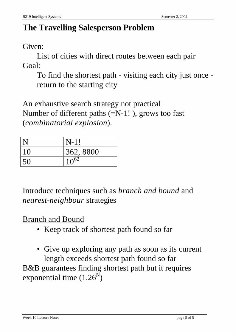
An exhaustive search strategy not practical Number of different paths (=N-1! ), grows too fast (combinatorial explosion). N N-1! 10 362, 8800 50 1062 Introduce techniques such as branch and bound and nearest-neighbour strategies Branch and Bound

• Keep track of shortest path found so far • Give up exploring any path as soon as its current

length exceeds shortest path found so far B&B guarantees finding shortest path but it requires exponential time (1.26N)



The Nearest-neighbour algorithm - an heuristic search method Works by selecting the locally superior alternative at each step Application of N-N algorithm to the travelling salesperson problem: 1. Select a starting city 2. Select the city closest to the current city. Visit the city 3. Repeat step 2 until all cities have been visited Executes in time proportional to N squared Does not guarantee the shortest path Heuristic algorithms does not guarantee to find the best solution but nearly always provide a very good answer Many heuristic algorithms, eg NN, provide an upper bound to the error (the maximum amount by which it will stray from the best answer)



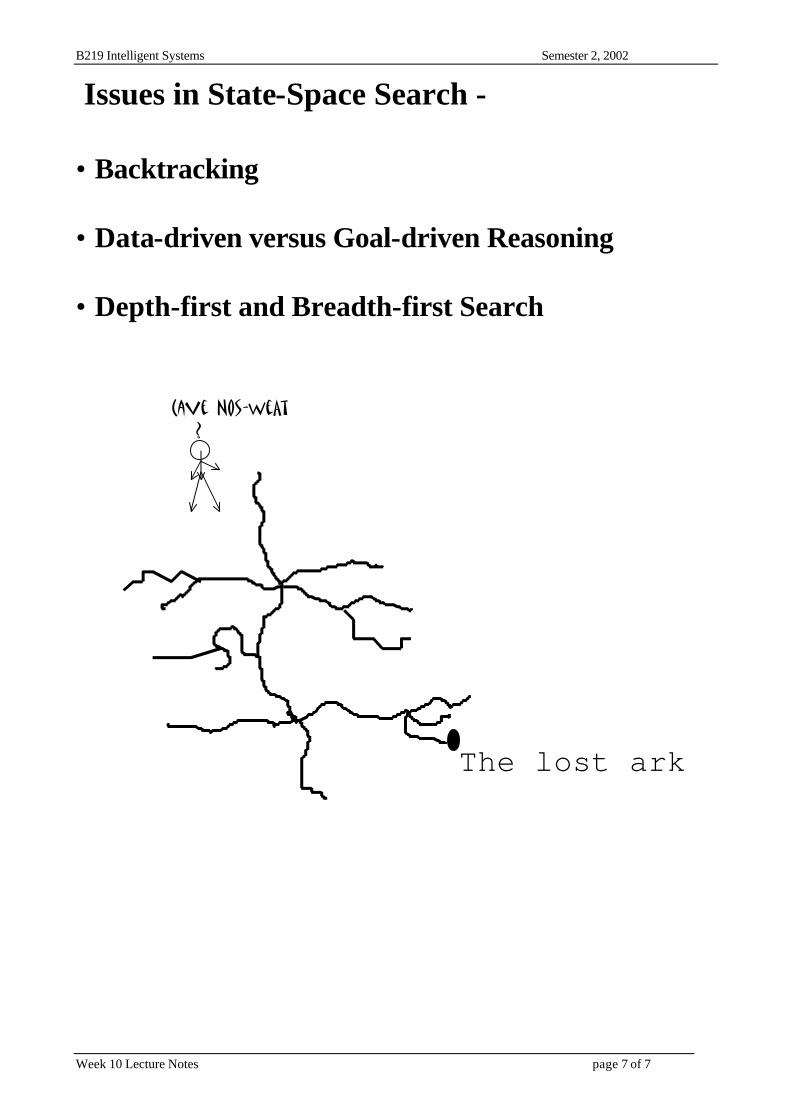
Issues in State-Space Search - • Backtracking • Data-driven versus Goal-driven Reasoning • Depth-first and Breadth-first Search Cave Nos-weAt ?

The lost ark



Backtracking A problem solver must find a path from start to goal through the state-space graph Backtracking enables recovery from mistakes Goal Initial state Backtracking search begins at the start state and pursues a path until it reaches either a goal or a dead end. If it finds a goal it quits and returns a solution path If it reaches a dead end, it backtracks to the most recent node unexamined



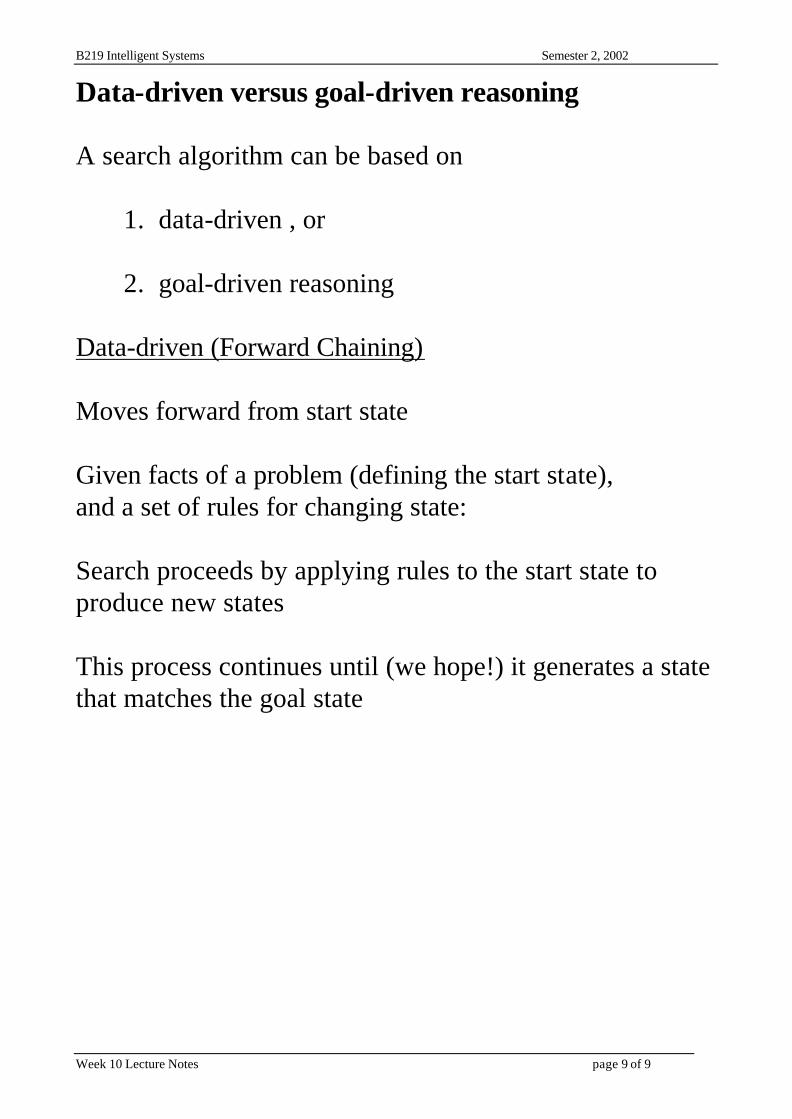
Data-driven versus goal-driven reasoning A search algorithm can be based on

1. data-driven , or 2. goal-driven reasoning

Data-driven (Forward Chaining) Moves forward from start state Given facts of a problem (defining the start state), and a set of rules for changing state: Search proceeds by applying rules to the start state to produce new states This process continues until (we hope!) it generates a state that matches the goal state



Goal-driven (Backward Chaining) Moves backward from goal state Finds what legal moves could be used to generate this goal Determines which state, when subjected to these moves generates the goal state This state becomes the new goal An example: The 8-puzzle Slide numbered tiles around to achieve the goal state

Start Goal 2 8 3 1 2 3

1 6 4 8 4

7 5 7 6 5



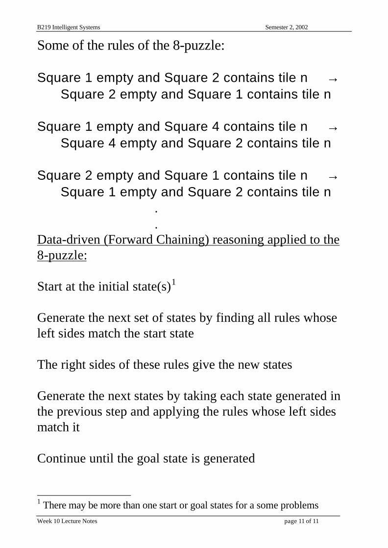
Some of the rules of the 8-puzzle: Square 1 empty and Square 2 contains tile n → Square 2 empty and Square 1 contains tile n Square 1 empty and Square 4 contains tile n → Square 4 empty and Square 2 contains tile n Square 2 empty and Square 1 contains tile n → Square 1 empty and Square 2 contains tile n . . Data-driven (Forward Chaining) reasoning applied to the 8-puzzle: Start at the initial state(s)1 Generate the next set of states by finding all rules whose left sides match the start state The right sides of these rules give the new states Generate the next states by taking each state generated in the previous step and applying the rules whose left sides match it Continue until the goal state is generated

1 There may be more than one start or goal states for a some problems



Goal-driven (Backward Chaining) reasoning applied to the 8-puzzle: Start at the goal state(s) Generate the next set of states by finding all rules whose right sides match the goal state The left sides of these rules give the new states Generate the next states by taking each state generated in the previous step and applying the rules whose right sides match it Continue until a node matching the start state is generated Should we reason forward or backward? • Are there more start states or goal states? - should move from the smaller set • In which direction is the branching factor greater? - take direction with lower branching factor • Will the program be asked to justify its reasoning process

to a user? - follow the user’s mode of reasoning



Depth-first and Breadth-first Search In state-space search, we need a strategy for selecting the order in which the next states will be examined At each step in the search process, we are faced with a number of alternative paths Two possible strategies: 1.We can explore one path at a time completely before

coming back and exploring other paths 2.We can explore all possible alternatives at the current

stage, before moving on.

When selecting a path, the alternatives must be remembered for later investigation if needed. We can use a tree to understand these two search strategies



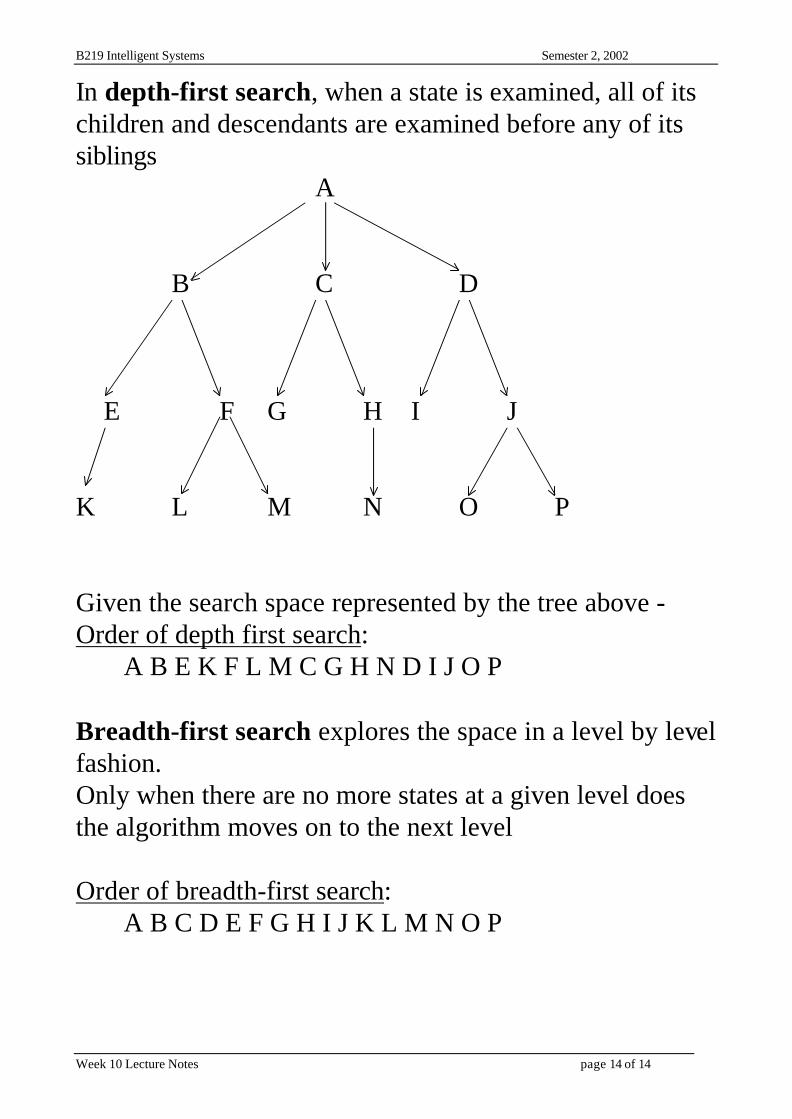
In depth-first search, when a state is examined, all of its children and descendants are examined before any of its siblings A B C D E F G H I J K L M N O P Given the search space represented by the tree above - Order of depth first search: A B E K F L M C G H N D I J O P Breadth-first search explores the space in a level by level fashion. Only when there are no more states at a given level does the algorithm moves on to the next level Order of breadth-first search: A B C D E F G H I J K L M N O P



Which search strategy to choose ?

- examine the problem space carefully

A comparison of breadth- and depth-first search: • B-F search guarantees a solution with the shortest path • D-F search more memory efficient - does not have to

remember all nodes at a level • D-F search may discover a path more quickly, if lucky • D- F search may get stuck with an infinite path



Production Systems A way of structuring AI programs for implementing search Defined by - 1. A set of rules (productions)

LHS of rule determines applicability of rule RHS describes action if the rule is applied Eg, a rule in the 8-puzzle problem Square 1 empty and Square 2 contains tile n → Square 2 empty and Square 1 contains tile n 2. A working memory (knowledge base) Contains info on current state & goal state Used to select a particular rule 3. The recognise-act-cycle Control strategy for the PS Finds matching rule & executes specified step Conflict resolution strategies select one rule if more than one match



A Production System Example - Sorting a string

Production Set: 1. ba → ab 2. ca → ac 3. cb → bc

Iteration # Working memory

Conflict set Rule fired

0 cbaca 1,2,3 1 1 cabca 3,2 2 2 acbac 1,3 1 3 acabc 2 2 4 aacbc 3 3 5 aacbc 3 3 6 aabcc 0 Halt

Fig. Trace of a simple production system A theory of human intelligence based on the PS model

Short-term memory equiv. to PS working memory Long-term memory holds all productions ST memory triggers LT memory’s productions



A production system example in Prolog - the Farmer, Wolf, Cabbage & Goat Problem Farmer F, Wolf W, Cabbage C and Goat G, must cross the river by boat from the West to the East side. Boat carries only two passengers (cabbage C counts as one!). G and W, or G and C must not be left together (“unsafe states”). What are the crossings to carry all four across safely? States of the problem space are represented using the predicate state(F,W,G,C) Initial state given by the fact state(w,w,w,w) What is the state after farmer takes cabbage across? Rule to operate on state with F and W on the same side to produce state with F and W on the other side move(state(X,X,G,C), state(Y,Y,G,C)) :-

opp(X,Y). opp(e,w). /* ensures e/w swap */ opp(w,e). /* ensures w/e swap */



The unsafe states may be represented by the rules /* wolf eats goat */ unsafe(state(X,Y,Y,C)) :- opp(X,Y). /* goat eats cabbage */ unsafe(state(X,W,Y,Y)) :- opp(X,Y). Using above rules to modify the move rule: /* farmer takes wolf to other side */ (1) move(state(X,X,G,C), state(Y,Y,G,C)) :-

opp(X,Y), not (unsafe(state(Y,Y,G,C))).

Similarly, /* farmer takes goat to other side */ (2) move(state(X,W,X,C), state(Y,W,Y,C)) :-

opp(X,Y), not (unsafe(state(Y,W,Y,C))). /* farmer takes cabbage to other side */ (3) move(state(X,W,G,X), state(Y,W,G,Y)) :-

opp(X,Y), not (unsafe(state(Y,W,G,Y))). /* farmer takes himself to other side */ (4) move(state(X,W,G,C), state(Y,W,G,C)) :-

opp(X,Y), not (unsafe(state(Y,W,G,C))).



A new state generated during the search may happen to be one already visited Search algorithms maintain a list of visited states to prevent looping We’ll first define a predicate path to determine if a path exists, using the recursive rule: For all X,Y [path(X,Y)]

←← There exists Z [(move(X,Z) ∧∧ path(Z,Y)]]

which states, “to find a path from state X to state Y, first move from starting state X to some intermediate state Z and then find a path from Z to Y” We now define predicate path with the list L of visited states as the third argument: path(Z,Z,L). /* a path from Z to Z always exists */ path(X,Y,L):- move(X,Z),

not(member(Z,L)), /* Z not visited */ path(Z,Y,[Z|L]). /* add Z to list */

The search terminates when the path generated leads to the goal state (successful) or loops back to the start state (failed)



Once a path to the goal state has been found, we do not want backtracking to generate further paths Generation of further solutions can be prevented by using the system predicate cut indicated by a ‘!’ (see Study Guide pp. 410-415) /* the recursive rule for finding path to goal */ path(State, Goal, List):-

move(State, NextState), not(member(NextState,List)), path(NextState,Goal,[NextState|List]),!. A fifth rule added to let the user know when the path call is backtracking /* No conditions, so always fires */ (5) move(state(F,W,G,C), state(F,W,G,C)):- writelist([‘ Backtrack from:’, F,W,G,C]),fail.



The production system for the FWGC problem opp(e,w). opp(w,e). /* farmer takes wolf to other side */ (1) move(state(X,X,G,C), state(Y,Y,G,C)) :-

opp(X,Y), not (unsafe(state(Y,Y,G,C))).

/* farmer takes goat to other side */ (2) move(state(X,W,X,C), state(Y,W,Y,C)) :- opp(X,Y), not (unsafe(state(Y,W,Y,C))). /* farmer takes cabbage to other side */ (3) move(state(X,W,G,X), state(Y,W,G,Y)) :- opp(X,Y), not (unsafe(state(Y,W,G,Y))). /* farmer takes himself to other side */ (4) move(state(X,W,G,C), state(Y,W,G,C)) :- opp(X,Y), not (unsafe(state(Y,W,G,C))). /* gets here when none of the above fires, system predicate ‘fail’ causes a backtrack*/ move(state(F,W,G,C), state(F,W,G,C)):- (5) writelist([‘ Backtrack from:’, F,W,G,C]), fail.



/* fires when the goal is reached - terminating condition*/ path(Goal, Goal, List):- write(‘Solution path is: ‘), nl, write(List). /* the recursive rule for finding path to goal */ path(State, Goal, List):-

move(State, NextState), not(member(NextState,List)), path(NextState,Goal,[NextState|List]),!. /* predicate "go" to test program */ go:- path(state(e,e,e,e),

state(w,w,w,w),[state(e,e,e,e)]). ?- go. [state(w,w,w,w),state(e,w,e,w),state(w,w,e,w), state(e,w,e,e),state(w,w,w,e),state(e,e,w,e), state(w,e,w,e),state(e,e,e,e)]



Heuristic Search In state-space search, heuristics are rules for choosing nodes in state space that are most likely to lead to a solution AI problem solvers employ heuristics in two basic situations 1.A problem may not have an exact solution

because of ambiguities in the problem statement or available data. Eg. medical diagnosis,

2.A problem has an exact solution, but computational

costs are high. Eg, the travelling salesperson problem - Straight forward brute force search impractical

Heuristics are fallible - only informed guess of the next step to be taken in problem solving. Thus cannot anticipate behaviour of state space further along the path Heuristics never guarantee the best solution, only expected to provide a good enough solution



An (heuristic) evaluation function at a given node gives an estimate (usually a number) of whether the node is on the desired path of solution Examples of simple evaluation functions Travelling salesman

sum of the distances so far

8-Puzzle number of tiles that are in the squares they belong

A high (eg, in 8-Puzzle) or a low ( eg, in Travelling salesman) value of the function may used in selecting the next state The cost of computing an accurate heuristic evaluation function may be too high In general, there is a trade-off between the cost of computing an evaluation function and the saving in search time



An example of the use of evaluation functions - Minimax Search A depth-first, depth-limited search procedure Objective:

Get the as reliable an e.f for a node in state space as possible

• Uses some rule to generate likely next states • Applies an evaluation function to these states • Backs up the best e.f. value to the parent state A (8) B C D (8) (3) (-2)

Fig.1 But, evaluation functions are not perfect Selecting state B may lead to an unfavourable state in the next step So, minimax search ‘looks ahead’ further down the tree and attempts to pass a better e.f. value up the tree



Let Min and Max be opponents in a game taking turns to make a move An e.f. value of 10 indicates a win for Max, -10 means win for Min Max’s move first

A B C D E F G H I J K (9) (-6) (0) (0) (-2) (-4) (-3)

Fig. 2

A (-2)

B (-6) C (-2) D (-4)

E F G H I J K (9) (-6) (0) (0) (-2) (-4) (-3)

Fig. 3 Note how the best move changes from ‘select node B’ (Fig.1) to ‘select node C’ (Fig.3) as Max looks ahead



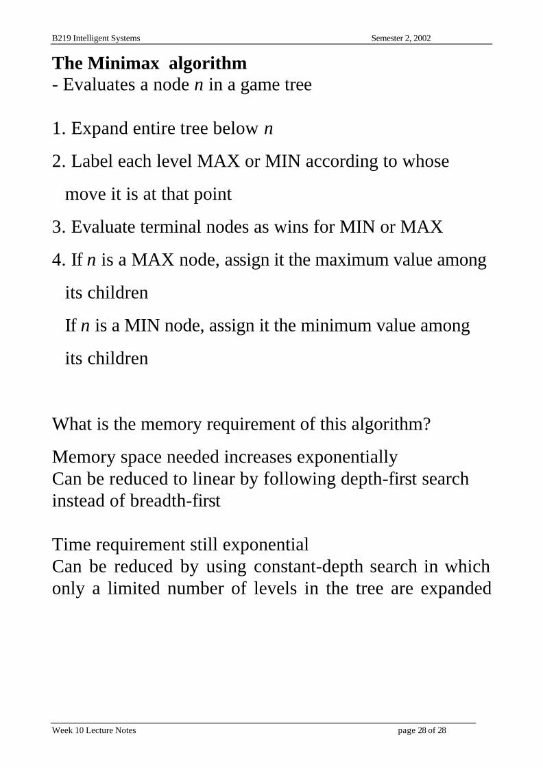
The Minimax algorithm - Evaluates a node n in a game tree 1. Expand entire tree below n

2. Label each level MAX or MIN according to whose

move it is at that point

3. Evaluate terminal nodes as wins for MIN or MAX

4. If n is a MAX node, assign it the maximum value among

its children

If n is a MIN node, assign it the minimum value among

its children

What is the memory requirement of this algorithm?

Memory space needed increases exponentially Can be reduced to linear by following depth-first search instead of breadth-first Time requirement still exponential Can be reduced by using constant-depth search in which only a limited number of levels in the tree are expanded



Increasing efficiency of Minmax search - Alpha-Beta Pruning Partial solutions clearly worse than already known solutions can be abandoned (branch-and-bound technique) A (>3) MAX B (3) C (<= -5) MIN D E F G MAX (3) (5) (-5)

Fig.4 Two thresholds are maintained: A lower bound (alpha) of the value a maximising node may assigned An upper bound (beta) of the value a minimising node may assigned In Fig. 4, no need to consider node G and its descendants - A will get a value of >= 3 in any case (how?)

Searching - what we have found so far In problem solving, we...

Documents

Transcript of Searching - what we have found so far In problem solving, we...