ISSN: 1439-2305

Number 321 – September 2017

SEARCHING FOR GROUPED PATTERNS

OF HETEROGENEITY IN THE

CLIMATE-MIGRATION LINK

Inmaculada Martinez-Zarzoso

1

Searching for Grouped Patterns of Heterogeneity

in the Climate-Migration Link

Inmaculada Martinez-Zarzoso*

University of Goettingen, Germany and Universidad Jaume I, Spain

Platz der Göttinger Sieben 3; 37073 Göttingen; Germany

Ph.: +49 551 399770; Fax: +49 551 398173

E-Mail: martinei@eco.uji.es

* Corresponding author: Inmaculada Martinez-Zarzoso, E-Mail: martinei@eco.uji.es. I would like to thank the organizers and the participants of the conference ‘Climate-Induced Migration’ held in FEEM, Milan for the very helpful comments and suggestions received.

2

Searching for Grouped Patterns of Heterogeneity in the Climate-Migration Link

Abstract

This paper uses international migration data and climate variables in a multi-country setting to

investigate the extent to which international migration can be explained by changes in the local

climate and whether this relationship varies between groups of countries. Moreover, the primary

focus is to further investigate the differential effect found by Cattaneo and Peri (2016) for

countries with different income levels using a high-frequency dataset. The idea being that country

grouping is considered to be data driven, instead of exogenously decided. The estimation

technique used to endogenously group the countries of origin is based on the group-mean fixed-

effects (GFE) estimator proposed by Bonhomme and Manresa (2015), which allows us to group

the origin countries according to the data generation process. The main results indicate that an

increasing average local temperature is associated with an increase in that country’s emigration

rate, on average, but the effect differs between groups. The results are driven by a group of

countries mainly located in Sub-Saharan Africa and Central Asia; however, no statistically

significant association is found between the average amount of local precipitation and that

country’s rate of emigration.

JEL Codes: F22, Q54

Key Words: international migration, climate change, developing countries, GFE, group

heterogeneity

1. Introduction

The impact of climate change on migration has been of concern since the early 1990s and

different points of view have been presented by environmentalists, economists and political

scientists. The discussion intensified with the publication of the fourth and fifth IPCC reports

(IPCC, 2007; IPCC, 2014) and during the multilateral climate negotiations that lead to the Paris

3

agreement and its implementation in November 2016. The IPCC (2007) report referred to the

“potential for population migration” due to climate distress. Although the topic has received

substantial media coverage, the academic research is still limited. While the standard statistical

migration literature has traditionally placed heavy emphasis on the socioeconomic drivers of

migration without considering climatic factors, a number of recent studies have focused on

natural disasters and extreme events as drivers of migration (Warner et al., 2009; Belasen and

Polachek, 2013; Drabo and Mbaye, 2015).

Very recently, a few economic studies have attempted to quantify the impacts on international

migration not only of extreme events, but also of changes in local temperature and precipitation

on a large scale (Backhaus et al., 2015; Beine and Parson, 2015; Cai et al., 2014; Coniglio et al,

2015 and Cattaneo and Peri, 2016). Whereas Beine and Parson (2015) focus mainly on extreme

weather events and temperature anomalies and Coniglio et al. (2015) focus on rainfall variability

in the sending countries, the other three papers focus on the effect of the average change in local

temperature on international migration. The main findings indicate that international migration

could be one of the responses to climate change, but the results vary by group of countries and

depend on the climatic variables used and on the time-span considered. There is also an important

difference in the approach of Cattaneo and Peri (2016) who focus on the global effect of

temperature changes on international emigration rates, without controlling for the effect of the

other determinants of international migration, and the remaining papers, which usually include

the economic-related determinants of international migration. The main result in Cattaneo and

Peri (2016) indicates that the effect of local temperature changes on emigration varies depending

on the average level of income of the sending countries. The authors group the countries

according to their income level and find that for middle-income countries, climatic warming is

associated with significantly higher emigration rates, whereas it is associated with lower rates in

4

poor countries where families cannot afford the cost of emigrating. We depart from Cattaneo and

Peri (2016) in that we propose to use a data-driven alternative method of grouping countries.

The main focus of this paper is to further investigate the differential effect found by Cattaneo and

Peri (2016) for high-frequency international migration data and for different country groups. The

main contribution of the study is that the country grouping is not exogenously decided but

obtained from the data. Grouped patterns of heterogeneity are consistent with the empirical

evidence that international migration patterns tend to be clustered in time and space. For instance,

there are waves of international migration induced by several factors that affect specific groups of

countries (e.g. conflict, natural disaster, etc.). The main estimation technique to endogenously

group the countries of origin is based on the group-mean fixed-effects estimator (GFE) proposed

by Bonhomme and Manresa (2015) that allows us to group the origin countries according to the

data generation process. After having found a suitable country grouping, a model for multi-origin

countries augmented with climate variables is estimated. The main data are taken from Backhaus

et al. (2015) and from Cattaneo and Peri (2016). We also replicate the results in Cattaneo and Peri

(2016) with high-frequency international migration data from Backhaus et al. (2015) to see if the

pattern they find is also valid for high-frequency data.

The results show that larger local temperature increases lead to an increase in emigration, on

average, but the effect differs between groups. The positive link is driven by a group of countries

located mainly in Sub-Saharan Africa and Central Asia, whereas no significant association is

found between the average local precipitation and emigration. Moreover, changes in local

precipitation levels also affect emigration differently between groups, but the effects are only

weakly statistically significant or non-significant. In the replication, we find that similar results

are obtained using yearly data and decadal data for the same sample of countries and using the

same model specification and estimation technique.

5

The rest of the paper is structured as follows. Section 2 summarizes the literature on international

migration and climate change. Section 3 refers to the related theoretical models and derives the

main empirical specification. Section 4 presents the empirical application, the main results and

the sensitivity analysis. Finally, Section 5 concludes.

2. Empirical Studies on Migration and Climatic Factors

In this section, we specifically focus on recent studies that consider domestic climatic factors to

be explanatory variables of migration. We refer to Belasen and Polachek (2013) and Backhaus et

al. (2015) for a summary of recent studies focusing on the more general socioeconomic

determinants of international migration and on environmental variables related to extreme events

and natural disasters. To introduce the impact of climate change and other economic variables

(income, trade, etc.) on migration in developing countries, we refer to the literature survey

presented in Lilleor and Van den Broeck (2011) and Choumert et al. (2015), which also refer to

mitigation and adaptation strategies.

Two early studies that focus on climatic factors are Barrios et al. (2006) and Marchiori et al.

(2012), which focus on internal and international migration, respectively. Both consider Sub-

Saharan African (SSA) countries as the main target area. Whereas the former study finds that

local rainfall shocks induce internal migration in SSA, but not in other developing countries, the

latter study finds some indirect effects of local rainfall and temperature anomalies that work

through the wage ratio and affect international migration.

Table 1 presents a review of the studies focused on the climate-migration link including a

summary of the main findings, the target climatic and migration variables used, the datasets and

the methodology applied in each study. Among the more recent studies, we can distinguish

between studies that use local average temperature and rainfall as the main climatic variables

(Backhaus et al., 2015; Cai et al., 2016; and Cattaneo and Peri, 2016) and those that focus on the

6

deviations of local rainfall and/or temperature from ‘normal’ levels (Beine and Parson, 2015; and

Coniglio et al., 2016).

Table 1. Summary of the literature on the migration-climate link

A second important characteristic of the studies is related to the migration data used. Whereas

some of them use data from 1960 to 2000 at ten-year intervals (Beine and Parson, 2015; and

Cattaneo and Peri, 2016), three of the very recent studies use yearly data starting in the 1980s or

1990s until the mid-2000s (Backhaus et al., 2015; Cai et al., 2014; and Coniglio et al, 2015).

Concerning the methodology used to estimate the statistical relationship between migration and

climate change, the authors that focus on bilateral migration use the gravity model of trade,

estimated with the most recent techniques proposed in the trade literature. Most of them include a

number of fixed effects to control for unobservable factors related to the destination country’s

migration policies, time-invariant origin country factors and to bilateral time-invariant factors

(Backhaus et al., 2015; Beine and Parsons, 2015; Cai et al., 2016; and Coniglio et al., 2016).

Beine and Parsons (2015) consider both natural disaster and climatic variation as potential drivers

of bilateral migration flows. Since their data provides information on migration in ten-year

intervals, their analysis is oriented towards the medium- and long-run effects of climate volatility.

Their results do not show any direct effect of the latter on international migration flows. It is

worth mentioning that they do not consider local average temperature and average precipitation

levels as done by Cai et al. (2016) and Cattaneo and Peri (2016), who do find a direct effect of

these climatic variables. Moreover, by using a large number of controls in the analysis of the

migration-climate relationship, it could be difficult to investigate the indirect effects of the

climatic variables on international migration. For this reason, as in Cattaneo and Peri (2016), we

7

focus on the global effect of local temperature on the emigration rate, without controlling for the

effect of other determinants of migration.

3. Theoretical Framework and Model Specification

We base our empirical model on the theoretical framework presented in Cattaneo and Peri

(2016), which is a ‘simple’ two period model that delivers a ‘hump-shaped’ relation between

migration rates and income per capita. Individuals work in the first period and earn the local

wage and in the second period decide whether or not to emigrate. It is assumed that individuals

cannot borrow; hence, they are only able to emigrate if they can pay for the monetary cost of

emigrating. The main predictions of the model are twofold. First, an increase in the local average

temperature is associated with an increase in the emigration rate in middle-income countries; and

secondly, for poor countries an increase in the local average temperature is associated with a

decrease in their emigration rate. The intuition behind this prediction is that in countries with

income below the median, the liquidity constraint is binding and prevents migration, while

individuals in countries with income above the median can afford the cost of migration and hence

are able to respond to adverse climate change by migrating.

We first replicate the results in Cattaneo and Peri (2016) with high-frequency migration data for

OECD immigration flows originating from developing countries.

The baseline empirical model is given by: ln = + + + ∗ ∑ + ∗∑ + + + +

(1)

8

where Mit is the immigration rate in OECD countries from country i in year t, which is defined as

the flow of migrants from country i to OECD destinations in year t divided by country i's

population in year t. The population‐weighted average annual temperature in degrees Celsius is

denoted as wtempit, while wpreit denotes average annual precipitation in millimeters. The use of

population weights makes the climate data more reflective of precisely how strongly the

inhabitants within a given country are actually affected by variations in local temperature and

precipitation, following the approach proposed by Dell et al. (2014). Dj is a set of dummies for

each quartile of the distribution of income and j=1…4. Hence, four different coefficients are

obtained for the variables of interest.

Alternatively, the variables are interacted with a dummy, dpoor, which takes the value of one if a

country’s income per capita is below the median. We include three sets of fixed effects (FE):

country FE (ζi), region-year FE (δrt) and interactions between the dummy for poor countries and

the year FE (γpt). Finally, uit denotes a random error term that is clustered at the country level in

the estimations.

In a second specification, we use the grouped fixed-effects (GFE) approach, which was recently

proposed by Bonhomme and Manresa (2015), to study the relationship between climatic factors

and migration flows over time and across countries. This statistical association has been recently

investigated and could become an important stylized fact. Consequently, it is important to

establish whether the relationship is heterogeneous across groups of countries. The GFE

estimation introduces time-varying grouped patters of heterogeneity in linear panel data models.

The estimator minimizes a least squares criterion with respect to all possible groupings of the

cross-sectional units. The most appealing feature of this approach is that group membership is left

unrestricted. The estimator is suitable for N big and T small and it is consistent as both

dimensions of the panel tend to infinity.

9

One of the most common approaches to model unobserved heterogeneity in panel data is the use

of time-invariant fixed-effects. This standard approach is sometimes subject to poorly estimated

elasticities when there are errors in the data or when the explanatory variables vary slowly over

time. Moreover, it is restrictive in that unobserved heterogeneity is assumed to be constant over

time. The GFE introduces clustered time patterns of unobserved heterogeneity that are common

within groups of countries. Both the group-specific time patterns and group membership are

estimated from the data.

Our benchmark specification is a linear model that explains migration, Mit, with grouped patterns

of heterogeneity and takes the form: ln = + +

where are the covariates that are assumed to be contemporaneously uncorrelated with the

error term, , but are allowed to be arbitrarily correlated with group-specific heterogeneity, . The countries in the same group share the same time profile and the number of groups is to be

decided or estimated by the researcher and group membership remains constant over time.

In essence, countries that have similar time profiles of migration –net of the explanatory

variables– are grouped together. The main underlying assumption is that group membership

remains constant over time.

The model can be easily modified to allow for additive time-invariant fixed effects, which is our

preferred specification1. We apply the within transformation to the dependent and independent

variables and estimate the model with variables in deviations with respect to the within-mean.

The new transformed variables are denoted as = − ̅ = − , .

The GFE in model (1) is the outcome of the minimization of the following expression:

1 The idea is to control not only for time-variant group-specific heterogeneity, but also for time-invariant country-specific unobserved heterogeneity.

10

, , = ∑ ∑ − −, , ∈

where the minimum of all possible groupings α={g1,…,gn} is taken of the N units in groups G,

parameters and group-specific time effects . The optimal group assignment for each country is

given by: , = ∑ − −∈ ,…,

Finally, the GFE estimates of beta and gamma are:

, = ∑ ∑ − − ,, ∈

where the GFE estimate of gi is , and the group probabilities are unrestricted and

individual-specific.

There are two algorithms available to minimize expression (5). The first one uses a simple

iterative strategy and is suitable for small-scale datasets, whereas the second, which exploits

recent advances in data clustering, is preferred for larger-scale problems. The former is used in

this paper.

Following the related literature, the model includes the two aforementioned climatic variables,

the average local temperature and precipitation rate. Meanwhile, the non-climate explanatory

variables derived from neoclassical theory, namely economic, demographic, geographic and

cultural controls as well as the trade-to-GDP ratio, are only included when investigating the

transmission channels of the migration-climate link. With this aim the specification considered is:

11

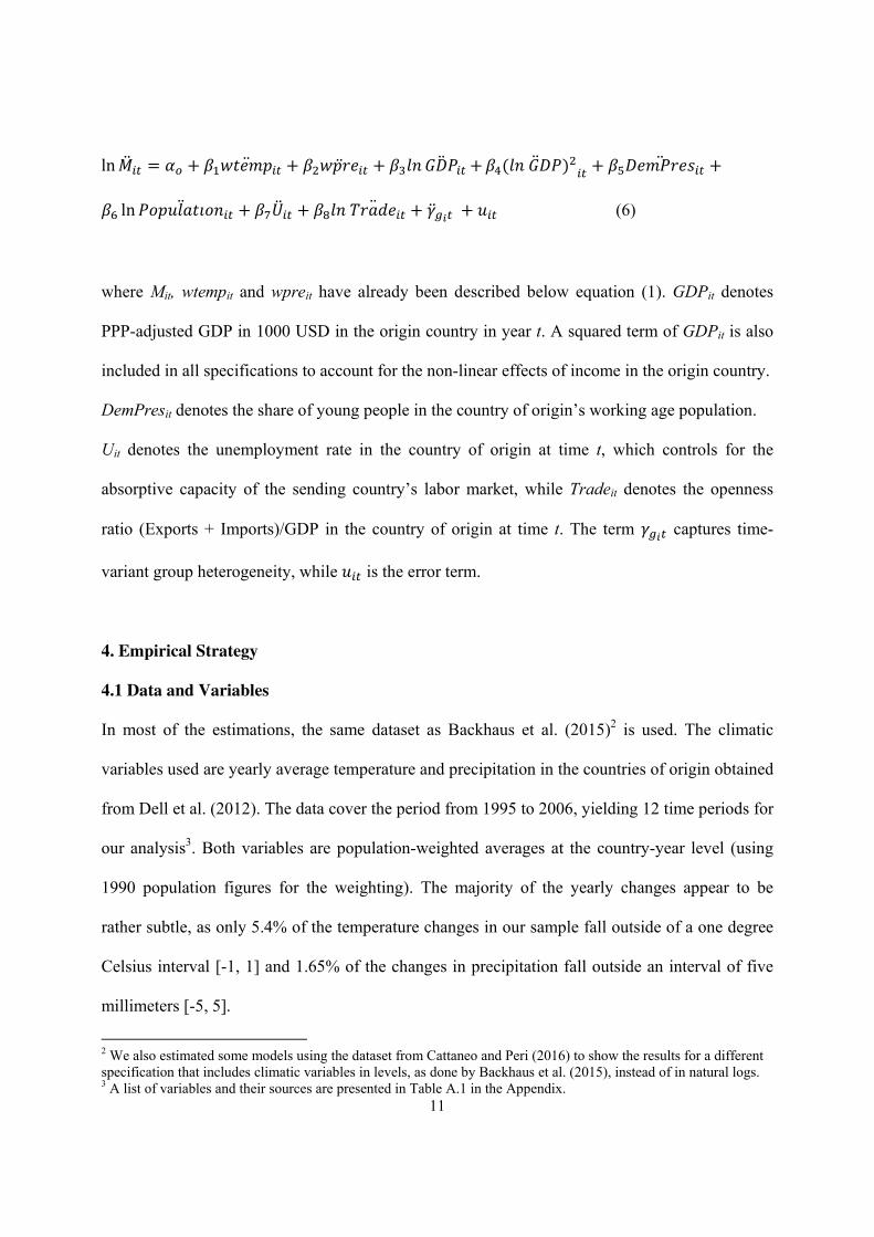
ln = + + + + + +ln + + + + (6)

where Mit, wtempit and wpreit have already been described below equation (1). GDPit denotes

PPP-adjusted GDP in 1000 USD in the origin country in year t. A squared term of GDPit is also

included in all specifications to account for the non-linear effects of income in the origin country.

DemPresit denotes the share of young people in the country of origin’s working age population.

Uit denotes the unemployment rate in the country of origin at time t, which controls for the

absorptive capacity of the sending country’s labor market, while Tradeit denotes the openness

ratio (Exports + Imports)/GDP in the country of origin at time t. The term captures time-

variant group heterogeneity, while is the error term.

4. Empirical Strategy

4.1 Data and Variables

In most of the estimations, the same dataset as Backhaus et al. (2015)2 is used. The climatic

variables used are yearly average temperature and precipitation in the countries of origin obtained

from Dell et al. (2012). The data cover the period from 1995 to 2006, yielding 12 time periods for

our analysis3. Both variables are population-weighted averages at the country-year level (using

1990 population figures for the weighting). The majority of the yearly changes appear to be

rather subtle, as only 5.4% of the temperature changes in our sample fall outside of a one degree

Celsius interval [-1, 1] and 1.65% of the changes in precipitation fall outside an interval of five

millimeters [-5, 5].

2 We also estimated some models using the dataset from Cattaneo and Peri (2016) to show the results for a different specification that includes climatic variables in levels, as done by Backhaus et al. (2015), instead of in natural logs. 3 A list of variables and their sources are presented in Table A.1 in the Appendix.

12

The corresponding data on yearly migration flows from the countries of origin to the destination

countries, originate primarily from the OECD’s International Migration Database (IMD, 2014). It

comprises 19 OECD members as destination countries on the basis of data availability, while

examining inflows from a maximum of 142 countries of origin. Some of the latter are members

of the OECD as well, e.g. Mexico, Chile and New Zealand. Although these countries might be

important destinations from the perspective of less developed countries, its role as a sending

country is also important. A complete list of the source and destination countries together with

their respective share of non-missing migration flow observations can be found in Table A.2 in

the Appendix. The IMD is constructed on the basis of statistical reports of the OECD member

countries, which implies that the data might not be fully comparable across countries, as the

criteria for registering an immigrant population and the conditions for granting residence permits

varies by country4. Regarding the European destination countries, data on inflows into Italy are

missing for many source countries and is completely unavailable for the years 1995-1997 and

2003. Observations from the Eurostat online database (Eurostat, 2014) were used to fill some of

the gaps. For Austria, Switzerland and the UK, numerous non-European source countries could

be added. Moreover, some rounded and inaccurate figures for the UK could be replaced. Adding

and replacing rounded observations was only done if the figures from the OECD and Eurostat

databases coincided for countries in which data was available in both databases. In this way, the

same definitions of immigration are used in both data sources and the consistency of the dataset

is not compromised by combining them. The data are mostly complete for France, Spain and

Germany, which together account for about sixty percent of the migratory flows to Europe in our

4 Illegal migration flows are only partially covered as data are only obtained through censuses. Furthermore, the majority of the destination countries did not record immigrants from the full set of source countries during the first few years of our period of analysis, as missing data are most frequent in this period. In the cases of Japan and the Republic of Korea, only the inflows from the most important regional sending countries have been recorded over a longer period of time.

13

sample; as well as for Australia, Canada and the United States, which reflects the long history of

immigration in these countries. With 12 years, 142 countries of origin and 19 countries of

destination, a dataset that is as comprehensive as possible on the immigration to OECD countries

is obtained by combining OECD and Eurostat information when possible.

Data for the economic and demographic variables are obtained from the World Bank’s World

Development Indicators (WDI, 2016) database. Table 1 presents summary statistics of the main

variables included in our model.

Table 2. Summary Statistics

4.2 Main Results

The migration models introduced in Section 3 are estimated for a wide sample of countries of

origin using yearly data from 1995 to 2006 from Backhaus et al. (2015). The first empirical

model (specification (1)) is also estimated using data from Cattaneo and Peri (2016), covering a

sample of 115 countries with information every ten years from 1990 to 2000.

Table 3 shows the results obtained from estimating specification (1). The first and second

columns present estimations obtained with Backhaus et al. (2016) data5 with the target variables

in levels and in natural logs, respectively. The results in the first column mostly present non-

significant coefficients at conventional levels, whereas the results in column 2 show different

signs and significance levels for the coefficients of the different income quartiles. More

specifically, for countries in the third quartile (fourth quartile), a 1 percent higher average

temperature in the countries of origin is associated with a 1.9 (1.6) percentage increase in the

emigration rate over one year, whereas countries in the first quartile who had a 1 percent higher

average temperature are associated with a decrease in the emigration rate of 4.5 percent.

5 We restrict the sample to developing countries, excluding high-income countries.

14

Furthermore, a decrease in the average precipitation rate in the countries of origin by 1 percent

corresponds to a 0.3 percentage increase in the emigration rate for the first quartile, whereas it

corresponds to a 0.2 percent decrease in the emigration rate in the second quartile. However, the

coefficient estimates for precipitation are imprecisely estimated. In column 3, the sample is

restricted to the 115 countries for which decade migration-stock data is available6. The results

stay similar to those in column 2, with the only difference being that the coefficients for the

weighted precipitation are statistically significant at the 5 percent level and therefore become

more accurate. Results for decade-data are presented in column (4), which is a replication of the

results found by Cattaneo and Peri (2016) –page 135, Table 2 (column 1) –. Although the

coefficients are not directly comparable, it is remarkable that the sign and statistical significance

of the estimates remain very similar in columns 3 and 4 for the coefficients of the weighted

temperature in each quartile and for the weighted precipitation. The only exception being for the

first quartile of the weighted precipitation, which is not statistically significant in column 4, but it

was at the 5% level in column 3. As expected, the coefficients are higher in magnitude using the

second sample, since they refer to changes over decades instead of to annual changes.

Overall, we obtain similar conclusions using high frequency data (annual) and decadal data.

Table 3. Parameter Estimates for the Benchmark Model

Next, we estimate a similar model using interactions of the climatic variables with a dummy

variable for countries with low income levels, using the definition from Cattaneo and Peri (2016)

of poor countries7. The results are presented in Table 4 for the specification with the climatic

6 This is done to compare the results using the same origin countries in both datasets. 7 Afghanistan, Benin, Burkina Faso, Burundi, Cambodia, the Central African Republic, the Democratic Republic of

Congo, Equatorial Guinea, Ethiopia, Gambia, Ghana, Guinea-Bissau, Lao People’s Democratic Republic, Lesotho,

15

variables in natural logarithms. Also in this case, the results for the weighted temperature

variables remain similar for both samples. However, for average precipitation, the interaction

with the poor dummy presents a negative coefficient, which is statistically significant in columns

2 and 3 for the yearly-data (sample B) but not for the decade-data (column 3). However, the

results for the average temperature are not robust to changes in the specification8.

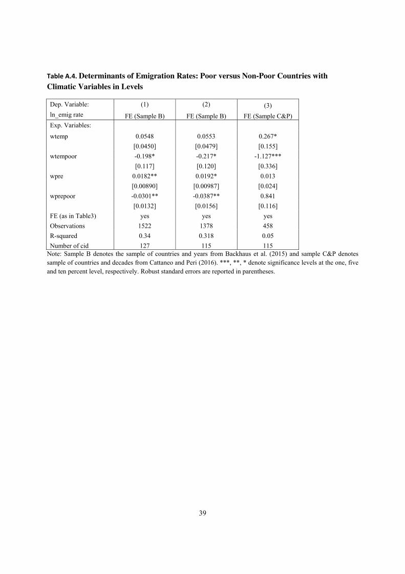
Table 4. Determinants of Emigration Rates. Poor versus Non-Poor Countries

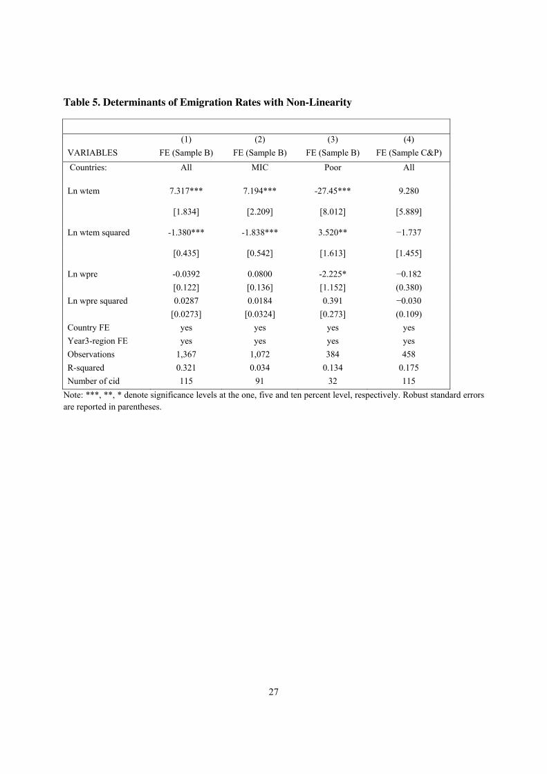
In Table 5, the relevance of non-linearity in the climatic variables is examined for the yearly-data

sample and compared with the decadal-data sample. The results in columns 1 to 3 show that there

is a non-linear relationship between the average temperature and the migration rate for all

countries (column 1), which vary by income level. While the relationship has an inverted-U

shape for middle-income countries (column 2), a U-shape curve is found for poor countries.

Using the C&P sample, the square terms are not statistically significant.

Table 5. Determinants of Emigration Rates with Non-Linearity

In our main empirical model, we allow the time-variant group effects to be correlated with

the explanatory variables9. Possible reasoning behind this assumption is that each group has its

own unobservable, time-varying mentality towards emigration that affects actual emigration rates

Liberia, Madagascar, Malawi, Mali, Mozambique, Nepal, Niger, Nigeria, Rwanda, Somalia, Sudan, the United Republic of Tanzania, Togo, Uganda, Yemen and Zambia. 8 When the model with the climatic variables in levels is estimated (Table A.4 in the Appendix), the weighted temperature variable is only statistically significant at the 10 percent level and only for poor countries (column 2) and for the low-frequency data the weighted temperature variable is only significant at the 10 percent level (column 3). 9 We only estimated this model with the low-frequency dataset, given that the GFE is more suitable for a panel with a time dimension that is not very small.

16

or that there exist specific relations between some source countries. The results are presented in

Table 6.

Table 6. Group Fixed Effects Estimation Results. Sample: Annual Data

The baseline GFE specification is presented in columns 1 and 2 of Table 6. The results in column

1 are obtained with the local climatic variables in levels10 and in column 2 in natural logs. In both

columns, the coefficient for average temperature is positive and statistically significant indicating

that higher average temperatures are associated with higher migration rates from developing

countries to OECD countries. The results for average precipitation indicate that lower

precipitation levels in the origin countries are associated with higher emigration rates, but the

corresponding estimate is only statistically significant at the 10 percent level for the model in

natural logs. Two additional specifications with non-linearity are estimated in columns 3 and 4.

Column 3 presents the results for a model in which the climatic variables are interacted with a

poor dummy variable, as was done in Table 4. With the GFE estimator, the results for the

average temperature indicate that only people from poor countries tend to emigrate at a higher

rate as a result of an increase in the average local temperature. Concerning the precipitation

variable, while decreasing precipitation induces migration in less-poor countries, in poor

countries decreasing precipitation is associated with decreasing emigration. This second outcome

is consistent with the ‘poverty trap’ argument.

The results in column 4 come from a model that includes the squared terms of the climatic

variables, as was done in Table 5. The results show that the squared term is only weakly relevant

for the average local temperature and precipitation. This could be the result of having specified

unobserved patterns of time-variant heterogeneity.

10 The estimated coefficient for the weighted temperature variable (in levels) was obtained by Backhaus et al. (2015) with a model for bilateral migration using a FE estimator. A number of control variables are also positive and statistically significant. The dependent variable in this case is the natural log of the migration bilateral flow.

17

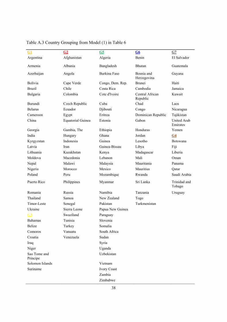
The GFE model presents the lowest RSME and the higher adjusted R-squared when the selected

number of groups is seven. Figure 2 shows a map with the country grouping and also a graph

with the time-variant patterns of heterogeneity. The list of countries in each group is shown in

Table A.3 in the Appendix.

In Table 7, we present results showing the group-specific coefficients for the climatic variables,

assuming that the groups remain constant over time. In column 1 of Table 7, only the average

temperature and the time group-specific variables are included in the model. Column 2 includes

only precipitation as a control variable while both sets of variables are included in column 3. The

results indicate that the positive relationship found for the average local temperature, and

migration from developing to developed countries, is driven by countries in group six, most of

which are located in Sub-Saharan Africa and Asia (see Table A.3 for a list of countries by group).

For group two, the coefficient for the average local temperature is negative and statistically

significant at the ten percent level. In this group, higher local temperatures are weakly associated

with decreases in the emigration rate. This group is composed of 10 countries in Africa, 5 in

South America, 4 in Eastern European, 4 in Central Asia, Indonesia, the Philippines and a few

small islands.

Table 7. Group-Specific Coefficients for Climatic Variables

Finally, we investigate the channels through which temperature operates on migration. We add a

number of controls to the model to see if the statistical significance of the climate variables

remains similar. In most cases, the addition of other controls does not alter the relationship, and

when it does, it is mainly due to the reduction of the sample size and not to the inclusion of

additional regressors.

Table 8. Transmission Channels

18

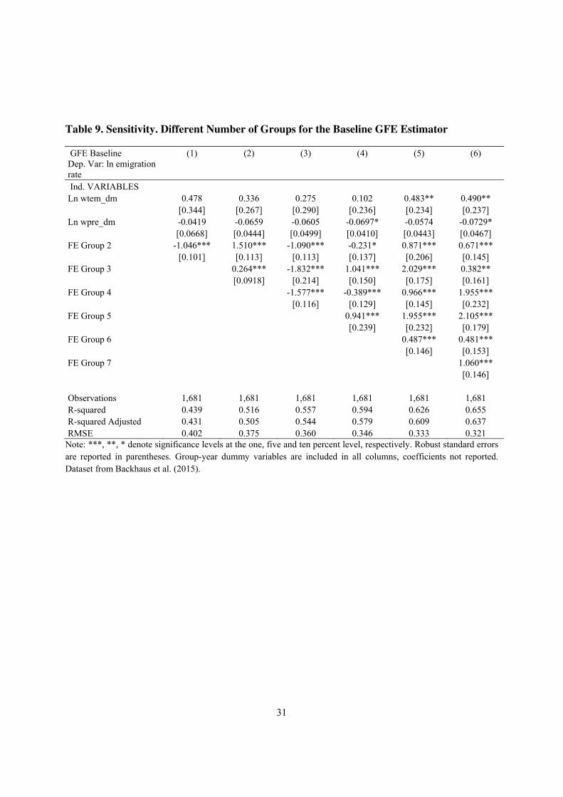
4.3 Sensitivity Analysis

We perform a series of sensitivity checks and explore some modifications of our basic model. In

each specification of Table 7 (in columns 1 to 4), we have estimated the model by varying the

number of groups. Table 9 presents an example of the estimations corresponding to the model in

column 2 (Table 7). Table 9 presents the results of applying the GFE estimator assuming a

different number of groups. We started with two groups (column 1) and increased the number

until the RMSE did not decrease any longer and the adjusted R-squared did not add any

additional explanatory power to the model. It can be observed that the results in columns 5 and 6,

which corresponds to groups six and seven, show very similar coefficients for the two target

variables. Furthermore, by increasing to 8 groups (not-shown), the results do not vary and the

additional group is very small in size11.

Secondly, we have estimated the GFE model restricting the sample to the countries considered by

Cattaneo and Peri (2016) and the country-grouping stays similar for the 115 remaining countries.

Finally, we have also estimated the model with the climatic variables in levels using the GFE

model and the results show slightly lower significance levels for the estimates. However, the

country-grouping remains very similar12.

Table 9. Migration Rate and Climatic Variables. Sensitivity Analysis

5. Concluding Remarks

11 Similar results, which are not reported, are obtained for the model in levels, with interaction and squared terms. In all cases, groups 7-8 provide the most suitable grouping according to statistical criteria (RMSE and adjusted R-squared). 12 Results from the second and third robustness checks are available upon request.

19

This paper documents a robust relationship between climatic variables and international

migration. In particular, increases in the average local temperature, and sometimes decreases in

the precipitation in a sending country, are associated with increases in international migration

flows especially for certain groups of countries. The main results obtained using the GFE

estimator, our preferred method, indicates that the effect is moderate, especially in relation to the

actual climatic variations in the high-frequency data. On average, a one percent increase in the

local temperature is associated with a 0.5 percent increase in the emigration rate for all countries,

whereas an increase of one percent in local precipitation is associated with a decrease in the

emigration of 0.07 percent. However, the effects are heterogeneous across country groups. The

endogenous grouping of the countries suggests that the reaction of emigration due to local

temperature changes might be driven by a group of sending countries mainly located in Sub-

Saharan Africa and Central Asia. More detailed studies of the countries in this group, exploiting

finer spatial variation in local precipitation and temperature, should be further investigated.

20

FIGURES

Figure 1. Emigration by Source

21

Figure 2. Map and Graph for Seven Groups (Model 2, Table 6)

Country Classification

-.5

0.5

11.5

1995 2000 2005year

Grouped Patterns

22

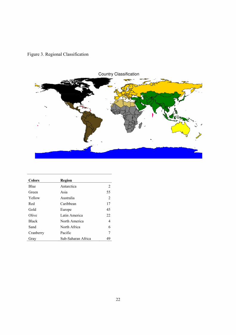
Figure 3. Regional Classification

Colors Region

Blue Antarctica 2

Green Asia 55

Yellow Australia 2

Red Caribbean 17

Gold Europe 45

Olive Latin America 22

Black North America 4

Sand North Africa 6

Cranberry Pacific 7

Gray Sub-Saharan Africa 49

Country Classification

23

TABLES

Table 1. Summary of the Literature on the Migration-Climate Link

Study Countries Period Method Migration type and

measure

Climate variables Main Finding

Barrios et al. (2006) 78 countries 1960‐1990 Cross‐country panel data

with country and time FE

Internal, Urbanization

as a proxy

Rainfall level normalized

by the mean

Rainfall shocks induce migration

in SSA only

Marchiori et al. (2012) 43 SSA countries 1960‐2000,

yearly basis

Cross‐country panel data

with country and time‐region FE

International, Net

migration rate

Precipitation and

temperature anomalies

Positive (negative) effect of

rainfall (temperature)

anomalies via wage ratio

Backhaus et al. (2015) 142 sending

countries to 19

OECD destinations

1995‐2006,

yearly basis

Gravity model with

country‐pair and time FE,

estimation in first

differences

International, Bilateral

migration inflows

Population‐weighted

Average temperature

and precipitation

Average temperature is

positively correlated with

bilateral migration, mainly for

agricultural‐depending

countries

Beine and Parson

(2015)

226 origin and

destination

countries

1960‐2000, ten

year intervals (5

waves)

Gravity model with origin

and destination‐time FE

(PPML)

International, Bilateral

migration rate

Natural disasters and

average deviations of

decadal average

temperature and

rainfall and anomalies

No evidence of direct impacts of

climate anomalies on

international migration but only

an indirect effect through wage

differentials

Coniglio and Pesce

(2015)

128 origin and 29

OECD destinations

(Listed in online

Appendix)

1990‐2001,

yearly basis

Gravity model with origin

and destination‐time FE

(PPML not reported)

International, Bilateral

migration inflows

Index of excess rainfall

variability

An increase in rainfall variability

(also in anomalies) is associated

with an increase in average

bilateral migration

Cai et al. (2016) 163 sending

countries to 42

destinations

1980‐2010,

yearly basis

Gravity model with

country‐pair and origin and

destination linear trends

International, Bilateral

migration rate

Population‐weighted

Average temperature

and precipitation

Each 1°C increase in

temperature implies a 5%

increase in out migration from

the top 25% agricultural

countries (significant at the 1%

level)

Cattaneo and Peri

(2016)

115 sending and

receiving

countries (30 poor

and 85 middle‐income) (Data in

online Appendix)

1960‐2000, ten

year intervals (5

waves)

Cross‐country panel data

with country and time‐region FE

International, Net

emigration flows (diff

between stocks in two

consecutive census)

from Ozden et al. (2011)

Population‐weighted

Average temperature

and precipitation from

Dell et al. (2012)

Climatic warming associated

with significantly higher

emigration rates in middle‐income countries and

significantly lower rates in poor

countries

Note: Author’s elaboration.

24

Table 2. Summary Statistics for the Dataset 1996-2008

Variable Obs. Mean Std. Dev. Min Max

Emigration rate 1,704 0.137 0.247 0 3.296

Ln emigration rate 1,693 -4.441 1.301 -8.238 -0.233

Weighted temperature 1,704 20.643 6.888 -1.562 29.583

Weighted Precipitation 1,704 10.910 7.415 0.066 40.567

GDP per capita 1000USD 1,605 5.580 7.922 0.123 65.182

Ln population 1,704 15.814 1.689 11.759 20.994

Demographic pressure 1,704 59.478 6.487 47.724 81.718

Stability 1,134 -0.369 0.925 -3.079 1.426

State fragility index 1,613 11.777 5.942 0 25

Unemployment rate 778 10.023 6.454 0.6 39.3

Max temperature 1,704 21.294 6.742 0.212 29.583

Min temperature 1,704 19.940 7.088 -1.562 28.495

Share_agriulture land 1,704 41.107 22.445 0.467 91.160

Steady wtemp change 1,278 0.128 0.335 0 1

Steady wpre change 1,278 0.095 0.293 0 1

Migration outflows 1,704 1370.405 2640.830 0 27828.830

Ln migration flows 1,693 4.474 1.614 0 8.652

Note: See Table A.1 in the Appendix for the definition of variables. ‘Weighted’ indicates that the corresponding

variable is population-weighted.

25

Table 3. Parameter Estimates for the Benchmark Model with Two Samples

Dep. Variable: (1) (2) (3) (4)

ln_emigration rate FE (Sample B) FE (Sample B) FE (Sample

countries C&P)

FE (Sample countries &

decades C&P)

Exp. Variables: no_ln ln ln ln

wtemp_initxtilegdp1 -0.162 -4.527** -4.842** -16.476***

[0.105] [2.154] [2.430] -6.25

wtemp_initxtilegdp2 -0.0247 0.828 1.564 7.474

[0.0924] [1.368] [1.198] -6.824

wtemp_initxtilegdp3 0.124* 1.947*** 2.086*** 8.614*

[0.0700] [0.734] [0.751] -5.143

wtemp_initxtilegdp4 0.0633 1.595*** 1.980*** 2.840**

[0.0639] [0.435] [0.527] -1.391

wpre_initxtilegdp1 -0.0157 -0.273* -0.335** -1.643

[0.0127] [0.156] [0.162] -1.902

wpre_initxtilegdp2 0.0204 0.256* 0.343** -1.684**

[0.0153] [0.142] [0.142] -0.658

wpre_initxtilegdp3 0.0163 0.0994 0.0474 0.097

[0.0163] [0.137] [0.137] -0.404

wpre_initxtilegdp4 0.00848 0.032 0.0182 0.434

[0.0124] [0.175] [0.207] -0.642

Country FE Yes Yes Yes Yes

Year (decade)-quartile FE Yes Yes Yes Yes

Year3 (decade)-region FE Yes Yes Yes Yes

Observations 1,522 1,511 1,367 458

R-squared 0.294 0.306 0.335 0.249

Number of countries 127 127 115 115

Note: Sample B denotes the sample of countries and years from Backhaus et al. (2015) and Sample C&P denotes the

sample from Cattaneo and Peri (2016). ***, **, * denote significance levels at the one, five and ten percent level,

respectively. Robust standard errors are reported in parentheses.

26

Table 4. Determinants of Emigration Rates Poor versus Non-Poor Countries

Dep. Variable: (1) (2) (3)

ln_emig rate FE (Sample B) FE (Sample B) FE (Sample C&P)

Ln wtem 1.706*** 1.946*** 3.755**

[0.408] [0.425] -0.661

Ln wtempoor -6.540*** -6.799*** -19.967***

[2.459] [2.468] -6.607

Ln wpre 0.0977 0.105 -0.223

[0.0946] [0.108] -0.325

Ln wprepoor -0.433** -0.440** -1.399

[0.187] [0.194] -1.912

FE (as in Table 3) yes yes yes

Observations 1511 1,367 458

R-squared 0.315 0.334 0.202

Number of cid 127 115 115

Note: Sample B denotes the sample of countries and years from Backhaus et al. (2015) and Sample C&P denotes the

sample of countries and decades from Cattaneo and Peri (2016). ***, **, * denote significance levels at the one, five

and ten percent level, respectively. Robust standard errors are reported in parentheses.

27

Table 5. Determinants of Emigration Rates with Non-Linearity

(1) (2) (3) (4)

VARIABLES FE (Sample B) FE (Sample B) FE (Sample B) FE (Sample C&P)

Countries: All MIC Poor All

Ln wtem 7.317*** 7.194*** -27.45*** 9.280

[1.834] [2.209] [8.012] [5.889]

Ln wtem squared -1.380*** -1.838*** 3.520** −1.737

[0.435] [0.542] [1.613] [1.455]

Ln wpre -0.0392 0.0800 -2.225* −0.182

[0.122] [0.136] [1.152] (0.380)

Ln wpre squared 0.0287 0.0184 0.391 −0.030

[0.0273] [0.0324] [0.273] (0.109)

Country FE yes yes yes yes

Year3-region FE yes yes yes yes

Observations 1,367 1,072 384 458

R-squared 0.321 0.034 0.134 0.175

Number of cid 115 91 32 115

Note: ***, **, * denote significance levels at the one, five and ten percent level, respectively. Robust standard errors

are reported in parentheses.

28

Table 6 Group Fixed Effects Estimation Results Sample Annual Data

(1) (2) (3) (4)

VARIABLES GFE_no ln GFE_ln GFE_ln GFE_ln

(ln) wtem_dm 0.0643*** 0.490** 0.390 -1.341

[0.0231] [0.237] [0.290] [1.145]

(Ln) wpre_dm 0.00175 -0.0729* -0.183*** -0.114*

[0.00501] [0.0467] [0.0558] [0.0582]

Ln wtempoor_dm 1.527**

[0.763]

Ln wprepoor_dm 0.318**

[0.133]

Ln wtem_squared_dm 0.444*

[0.265]

Ln wpre_squared_dm 0.0283*

[0.0162]

FE Group 2 -0.142 0.671*** -0.203* 1.912***

[0.156] [0.145] [0.107] [0.216]

FE Group 3 -0.299*** 0.382** 1.196*** -0.771***

[0.0846] [0.161] [0.122] [0.155]

FE Group 4 -0.976*** 1.955*** 0.0631 0.225**

[0.142] [0.232] [0.282] [0.0884]

FE Group 5 -0.588*** 2.105*** 0.125 -0.312***

[0.111] [0.179] [0.110] [0.108]

FE Group 6 0.969*** 0.481*** 1.921*** 0.922***

[0.196] [0.153] [0.205] [0.135]

FE Group 7 1.001*** 1.060*** 0.206 1.197***

[0.127] [0.146] [0.130] [0.119]

FE Group 8 0.143

[0.157]

Observations 1,693 1,681 1,681 1,681

R-squared 0.676 0.655 0.660 0.679

R-squared Adjusted 0.657 0.637 0.639 0.659

RMSE 0.312 0.321 0.327 0.311

Note: ***, **, * denote significance levels at the one, five and ten percent level, respectively. Robust standard errors

are reported in parentheses. Group-year dummy variables are included in all columns, coefficients not reported.

29

Table 7. Group-Specific Coefficients for Climatic Variables

(1) (2) (3)

VARIABLES FE FE FE

Ln wtem g1 0.0411 0.00883

[0.310] [0.325]

Ln wtem g2 -0.693* -0.733*

[0.399] [0.403]

Ln wtem g3 2.536 0.533

[8.313] [9.632]

Ln wtem g4 3.343 2.670

[2.715] [2.603]

Ln wtem g5 0.752 0.760

[0.688] [0.777]

Ln wtem g6 2.284** 2.410**

[1.004] [0.960]

Ln wtem g7 -1.526 -1.922

[1.271] [1.437]

Ln wpre g1 -0.0488 -0.0808

[0.102] [0.107]

Ln wpre g2 -0.0935 -0.0970

[0.0990] [0.0952]

Ln wpre g3 0.262** 0.259

[0.103] [0.165]

Ln wpre g4 -0.166 -0.126

[0.122] [0.122]

Ln wpre g5 -0.0119 0.00418

[0.0770] [0.0859]

Ln wpre g6 -0.00904 0.0669

[0.176] [0.182]

Ln wpre g7 -0.113 -0.142

[0.104] [0.108]

Observations 1,573 1,584 1,573

R-squared 0.654 0.652 0.655

Number of cid 133 133 133

Note: ***, **, * denote significance levels at the one, five and ten percent level, respectively. Robust standard errors

are reported in parentheses. Group-year dummy variables are included in all columns, coefficients not reported.

30

Table 8. Transmission Channels

(1) (2) (3) (4) (5) (6) (7)

VARIABLES FE FE FE FE FE FE FE

lnwtemg1 0.217 0.242 0.0117 -0.0963 0.123 0.00843 -0.0155

[0.299] [0.300] [0.325] [0.370] [0.397] [0.326] [0.317]

lnwtemg2 -0.703* -0.621* -0.742* -1.113** -0.0618 -0.733* -0.767*

[0.417] [0.344] [0.407] [0.437] [0.276] [0.403] [0.420]

lnwtemg3 1.435 -0.554 0.509 9.256 -47.53*** 0.533 0.490

[9.465] [9.464] [9.634] [6.361] [0.0808] [9.635] [9.608]

lnwtemg4 2.369 2.477 2.675 6.224** 1.851 2.670 2.685

[2.838] [2.580] [2.617] [2.721] [2.034] [2.604] [2.610]

lnwtemg5 0.189 0.334 0.754 0.553 0.0591 0.762 0.756

[0.623] [0.688] [0.780] [0.949] [0.557] [0.777] [0.777]

lnwtemg6 2.485** 2.405** 2.429** 1.750 5.600*** 2.384** 2.401**

[1.003] [0.964] [0.972] [1.140] [1.610] [0.959] [0.962]

lnwtemg7 -1.819 -2.219 -1.900 -4.081** 0.242 -1.922 -1.923

[1.450] [1.432] [1.437] [1.666] [8.538] [1.437] [1.430]

lnwpreg1 -0.126 0.0359 -0.0822 -0.261 0.0857 -0.0808 -0.0870

[0.126] [0.0915] [0.110] [0.179] [0.117] [0.107] [0.106]

lnwpreg2 -0.0987 -0.0836 -0.0997 -0.119 0.0509 -0.0986 -0.0989

[0.0962] [0.103] [0.0980] [0.0998] [0.0425] [0.0952] [0.0963]

lnwpreg3 0.282 0.267* 0.259 0.308** -2.206*** 0.259 0.263

[0.182] [0.154] [0.165] [0.120] [0.0544] [0.165] [0.166]

lnwpreg4 -0.152 -0.116 -0.127 0.411** 0.0225 -0.126 -0.126

[0.144] [0.120] [0.122] [0.178] [0.160] [0.122] [0.122]

lnwpreg5 -0.0317 0.00954 0.00547 0.0610 0.133 0.00506 0.00297

[0.109] [0.101] [0.0857] [0.0591] [0.115] [0.0860] [0.0859]

lnwpreg6 0.0190 0.0673 0.0684 0.229 0.0676 0.0635 0.0677

[0.164] [0.183] [0.181] [0.210] [0.160] [0.182] [0.182]

lnwpreg7 -0.146 -0.175 -0.145 -0.344 0.0514 -0.142 -0.145

[0.109] [0.107] [0.109] [0.232] [0.201] [0.108] [0.108]

log_gdpcap_origin -0.128

[0.113]

trade_to_gdp 0.000219

[0.000753]

demographic_pressure -0.00407

[0.0125]

stability -0.0258

[0.0378]

unemployment_origin 0.00203

[0.00483]

share_tsunami_deaths -1.236***

[0.296]

share_agricultural_land -0.00285

[0.00610]

Observations 1,484 1,492 1,573 1,050 720 1,573 1,573

R-squared 0.667 0.669 0.655 0.629 0.733 0.656 0.655

Number of cid 127 129 133 133 108 133 133

31

Table 9. Sensitivity. Different Number of Groups for the Baseline GFE Estimator

GFE Baseline (1) (2) (3) (4) (5) (6) Dep. Var: ln emigration rate

Ind. VARIABLES

Ln wtem_dm 0.478 0.336 0.275 0.102 0.483** 0.490**

[0.344] [0.267] [0.290] [0.236] [0.234] [0.237]

Ln wpre_dm -0.0419 -0.0659 -0.0605 -0.0697* -0.0574 -0.0729*

[0.0668] [0.0444] [0.0499] [0.0410] [0.0443] [0.0467]

FE Group 2 -1.046*** 1.510*** -1.090*** -0.231* 0.871*** 0.671***

[0.101] [0.113] [0.113] [0.137] [0.206] [0.145]

FE Group 3 0.264*** -1.832*** 1.041*** 2.029*** 0.382**

[0.0918] [0.214] [0.150] [0.175] [0.161]

FE Group 4 -1.577*** -0.389*** 0.966*** 1.955***

[0.116] [0.129] [0.145] [0.232]

FE Group 5 0.941*** 1.955*** 2.105***

[0.239] [0.232] [0.179]

FE Group 6 0.487*** 0.481***

[0.146] [0.153]

FE Group 7 1.060***

[0.146]

Observations 1,681 1,681 1,681 1,681 1,681 1,681

R-squared 0.439 0.516 0.557 0.594 0.626 0.655

R-squared Adjusted 0.431 0.505 0.544 0.579 0.609 0.637

RMSE 0.402 0.375 0.360 0.346 0.333 0.321

Note: ***, **, * denote significance levels at the one, five and ten percent level, respectively. Robust standard errors

are reported in parentheses. Group-year dummy variables are included in all columns, coefficients not reported.

Dataset from Backhaus et al. (2015).

32

Acknowledgements

Financial support from the Spanish Ministry of Economy and Competitiveness is gratefully

acknowledged (ECO2014-58991-C3-2-R). We would also like to thank the participants of the

workshop held in FEEM, Milan for their helpful comments and suggestions.

References

Backhaus, Andreas, Martinez-Zarzoso, Inma and Muris, Chris (2015) Do climate variations

explain bilateral migration? A gravity model analysis, IZA Journal of Migration 4(3), 1-15.

Barrios, Salvador, Luisito Bertinelli and Eric Strobl (2006) Climatic change and rural-urban

migration: The case of sub-Saharan Africa, Journal of Urban Economics 60, 357-371.

Beine, Michel and Christopher Parsons (2015) Climatic Factors as Determinants of International

Migration, Scandinavian Journal of Economics 117 (2), 723-767.

Belasen, Ariel R. and Solomon W. Polachek (2013) Natural disasters and migration, in The

International Handbook on the Economics of Migration, Amelie F. Constant and Klaus F.

Zimmermann (editors), Edward Elgar Publishing: Cheltenham, UK, Chapter 17, 309-330.

Bonhomme, Stéphan and Manresa, Elena (2015) Grouped patterns of heterogeneity in panel data.

Econometrica 83 (3), 1147–1184.

Cai, Ruohong, Shuaizhang Feng, Mariola Pytliková and Michael Oppenheimer (2016) Climate

Variability and International Migration: The Importance of the Agricultural Linkage, Journal of

Environmental Economics and Management 79, 135-151.

Cattaneo, Cristina and Giovanni Peri (2016) The migration response to increasing temperatures,

Journal of Development Economics, 122, 127-146.

33

Choumert, Johanna, Pascale Combes Motel, Katrin Millock (2015) Climate change mitigation

and adaptation in developing and transition countries: introduction to the special issue,

Environment and Development Economics 20 (04), 425-427.

Coniglio, Nicola D. and Pesce, Giovanni (2015) Climate variability and international Migration:

An empirical analysis, Environment and Development Economics 20 (4), 436-468.

Dell, Melissa, Benjamin F. Jones and Benjamin A. Olken (2012) “Temperature Shocks and

Economic Growth: Evidence from the Last Half Century”, American Economic Journal

Macroeconomics 4 (3), 66-95.

Dell, Melissa, Benjamin F. Jones and Benjamin A. Olken (2014) What Do We Learn from the

Weather? The New Climate-Economy Literature, Journal of Economic Literature, 52(3), 740-98.

Drabo A. and L. M. Mbaye (2015) Natural disasters, migration and education: an empirical

analysis in developing countries, Environment and Development Economics 20, 767-796.

IPCC (2007): Climate Change 2007: Synthesis Report. Contribution of Working Groups I, II and

III to the Fourth Assessment Report of the Intergovernmental Panel on Climate Change, [Core

Writing Team, Pachauri, R.K and Reisinger, A. (eds.)], IPCC, Geneva, Switzerland.

IPCC (2014): Climate Change 2014: Synthesis Report. Contribution of Working Groups I, II and

III to the Fifth Assessment Report of the Intergovernmental Panel on Climate Change, [Core

Writing Team, Pachauri, R.K and Meyer, L. A. (eds.)], IPCC, Geneva, Switzerland.

Lilleor, Helene B. and Van den Broeck, Katleen (2011) Economic drivers of migration and

climate change on LDCs, Global Environmental Change 21(Supplement 1), S70-S81.

34

Marchiori, Luca, Jean-François Maystadt, Ingmar Schumacher (2012) The impact of weather

anomalies on migration in sub-Saharan Africa, Journal of Environmental Economics and

Management 63 (3), 355–374.

Millock, Katrin (2015) Migration and Environment, Annual Review of Resource Economics 7 (1)

35-60.

Reuveny, Rafael (2007) Climate change-induced migration and violent conflict, Political

Geography, 26 (6), 656-673.

Reuveny, Rafael and Will H. Moore (2009) Does Environmental Degradation Influence

Migration? Emigration to Developed Countries in the late 1980s and early 1990s, Social Science

Quarterly, 90 (3), 461-479.

Warner, Koko, Marc Stal, Olivia Dun amd Tamer Afifi (2009) Researching environmental

change and migration: Evaluation of EACH-FOR methodology and application in 23 case studies

worldwide, in Migration, Environment and Climate Change: Assessing the Evidence, Frank

Laczko and Christine Aghazarm (editors), IOM, Geneva, 197-244.

35

APPENDIX

Table A.1. List of Variables, Definitions and Sources

Variable Definition Source

Weighted

temperature (wtemp)

Population‐weighted average annual temperature in degrees Celsius

in country i. Constant 1990 population weights Dell et al. (2012)

Weighted

precipitation (wpre)

Population‐weighted average annual precipitation in millimeters in

country i. Constant 1990 population weights Dell et al. (2014)

Migration flow Inflow of population from sending country i

Organization for Economic Co-operation and Development (2014): OECD International Migration Database.

Eurostat (2014): Immigration.

GDP per capita PPP-adjusted GDP per capita in sending country at current US$ World Bank (2014): World Development Indicators Database.

Population Population in the sending country World Bank (2014): World Development Indicators Database.

Demographic

pressure

Percentage or young population as a share of working

age population in the sending country World Bank (2014): World Development Indicators Database.

Unemployment rate

Unemployment rate in the country of destination, total

(share of total labor force) World Bank (2014): World Development Indicators Database.

Trade to GDP Sum of exports and imports of goods and services measured as a share of the sending country’s gross domestic product

World Bank (2014): World Development Indicators Database.

Share of agricultural

land

Share of sending country i's land area that is arable, under permanent crops, and under permanent pastures

World Bank (2014): World Development Indicators Database.

State fragility index Ordinally scaled (0-25) measure of sending country i’s state fragility Center for Systemic Peace (2014): State Fragility Index.

36

Table A.2. List of Countries

Destination Countries

Australia 0.76 France 0.82 Norway 0.84

Austria 0.6 Germany 0.88 Portugal 0.08

Belgium 0.11 Italy 0.28 Spain 0.69

Canada 0.86 Japan 0.13 Sweden 0.57

Denmark 0.57 Korea 0.03 Switzerland 0.7

Finland 0.5 Netherlands 0.69 United Kingdom 0.39 United States 0.82

Countries of Origin

Afghanistan 0.64 Fiji 0.45 Nigeria 0.64

Albania 0.61 Gabon 0.37 Oman 0.45

Algeria 0.65 Gambia 0.56 Pakistan 0.74

Angola 0.61 Georgia 0.57 Panama 0.52

Argentina 0.62 Ghana 0.64 Papua New Guinea 0.29

Armenia 0.57 Guatemala 0.54 Paraguay 0.49

Azerbaijan 0.57 Guinea 0.54 Peru 0.64

Bahamas 0.36 Guinea-Bissau 0.46 Philippines 0.83

Bangladesh 0.67 Guyana 0.49 Poland 0.78

Belarus 0.57 Haiti 0.46 Puerto Rico 0.02

Belize 0.36 Honduras 0.54 Qatar 0.28

Benin 0.44 Hungary 0.62 Romania 0.76

Bhutan 0.4 India 0.79 Russian Federation 0.85

Bolivia 0.57 Indonesia 0.69 Rwanda 0.57

Bosnia & Herzegovina 0.69 Iran 0.7 Samoa 0.2

Botswana 0.46 Iraq 0.67 Sao Tome&Principe 0.22

Brazil 0.8 Jamaica 0.6 Saudi Arabia 0.52

Brunei Darussalam 0.3 Jordan 0.6 Senegal 0.6

Bulgaria 0.68 Kazakhstan 0.57 Sierra Leone 0.54

Burkina Faso 0.48 Kenya 0.6 Slovenia 0.57

Burundi 0.53 Kuwait 0.43 Solomon Islands 0.11

Cambodia 0.55 Kyrgyzstan 0.53 Somalia 0.68

Cameroon 0.61 Laos 0.51 South Africa 0.59

Cape Verde 0.46 Latvia 0.59 Sri Lanka 0.68

Central African Rep. 0.32 Lebanon 0.66 Sudan 0.57

Chad 0.36 Lesotho 0.31 Suriname 0.37

Chile 0.6 Liberia 0.54 Swaziland 0.37

China 0.86 Libya 0.56 Syria 0.63

Colombia 0.63 Lithuania 0.6 Tajikistan 0.47

Comoros 0.2 Macedonia FYR 0.56 Tanzania 0.59

Congo, Dem. Rep. 0.55 Madagascar 0.5 Thailand 0.82

Congo, Rep. 0.5 Malawi 0.5 Timor-Leste 0.08

37

Costa Rica 0.52 Malaysia 0.61 Togo 0.54

Côte d'Ivoire 0.58 Mali 0.46 Trinidad and Tobago 0.57

Croatia 0.64 Mauritania 0.46 Tunisia 0.66

Cuba 0.56 Mauritius 0.59 Turkey 0.79

Cyprus 0.57 Mexico 0.63 Turkmenistan 0.43

Czech Republic 0.61 Moldova 0.61 Uganda 0.57

Djibouti 0.43 Mongolia 0.54 Ukraine 0.69

Dominican Republic 0.58 Morocco 0.6 United Arab Emirates 0.44

Ecuador 0.62 Mozambique 0.55 Uruguay 0.52

Egypt 0.64 Myanmar 0.51 Uzbekistan 0.57

El Salvador 0.53 Namibia 0.5 Vanuatu 0.14

Equatorial Guinea 0.22 Nepal 0.57 Venezuela 0.68

Eritrea 0.54 New Zealand 0.62 Viet Nam 0.79

Estonia 0.6 Nicaragua 0.54 Yemen 0.5

Ethiopia 0.64 Niger 0.49 Zambia 0.57

Zimbabwe 0.56

Note: The numbers denote the share of non-missing observations.

38

Table A.3 Country Grouping from Model (1) in Table 6

G1 G2 G5 G6 G7

Argentina Afghanistan Algeria Benin El Salvador

Armenia Albania Bangladesh Bhutan Guatemala

Azerbaijan Angola Burkina Faso Bosnia and Herzegovina

Guyana

Bolivia Cape Verde Congo, Dem. Rep. Brunei Haiti

Brazil Chile Costa Rica Cambodia Jamaica

Bulgaria Colombia Cote d'Ivoire Central African Republic

Kuwait

Burundi Czech Republic Cuba Chad Laos

Belarus Ecuador Djibouti Congo Nicaragua

Cameroon Egypt Eritrea Dominican Republic Tajikistan

China Equatorial Guinea Estonia Gabon United Arab Emirates

Georgia Gambia, The Ethiopia Honduras Yemen

India Hungary Ghana Jordan G4

Kyrgyzstan Indonesia Guinea Lesotho Botswana

Latvia Iran Guinea-Bissau Libya Fiji

Lithuania Kazakhstan Kenya Madagascar Liberia

Moldova Macedonia Lebanon Mali Oman

Nepal Malawi Malaysia Mauritania Panama

Nigeria Morocco Mexico Mauritius Qatar

Poland Peru Mozambique Rwanda Saudi Arabia

Puerto Rico Philippines Myanmar Sri Lanka Trinidad and Tobago

Romania Russia Namibia Tanzania Uruguay

Thailand Samoa New Zealand Togo

Timor-Leste Senegal Pakistan Turkmenistan

Ukraine Sierra Leone Papua New Guinea

G3 Swaziland Paraguay

Bahamas Tunisia Slovenia

Belize Turkey Somalia

Comoros Vanuatu South Africa

Croatia Venezuela Sudan

Iraq Syria

Niger Uganda

Sao Tome and Principe

Uzbekistan

Solomon Islands Vietnam

Suriname Ivory Coast

Zambia

Zimbabwe

39

Table A.4. Determinants of Emigration Rates: Poor versus Non-Poor Countries with

Climatic Variables in Levels

Dep. Variable: (1) (2) (3)

ln_emig rate FE (Sample B) FE (Sample B) FE (Sample C&P)

Exp. Variables:

wtemp 0.0548 0.0553 0.267*

[0.0450] [0.0479] [0.155]

wtempoor -0.198* -0.217* -1.127***

[0.117] [0.120] [0.336]

wpre 0.0182** 0.0192* 0.013

[0.00890] [0.00987] [0.024]

wprepoor -0.0301** -0.0387** 0.841

[0.0132] [0.0156] [0.116]

FE (as in Table3) yes yes yes

Observations 1522 1378 458

R-squared 0.34 0.318 0.05

Number of cid 127 115 115

Note: Sample B denotes the sample of countries and years from Backhaus et al. (2015) and sample C&P denotes

sample of countries and decades from Cattaneo and Peri (2016). ***, **, * denote significance levels at the one, five

and ten percent level, respectively. Robust standard errors are reported in parentheses.