Search and Rest Unemployment∗

Fernando Alvarez

University of Chicagof-alvarez1@uchicago.edu

Robert Shimer

University of Chicagorobert.shimer@gmail.com

May 4, 2009

Abstract

This paper develops a tractable version of the Lucas and Prescott (1974) search

model. The economy consists of a continuum of labor markets, each of which produces

a heterogeneous good which are imperfect substitutes. There is a constant returns to

scale production technology in each labor market, but productivity is continually hit

by idiosyncratic shocks, inducing the costly reallocation of workers across markets. In

equilibrium, some workers search for new labor markets while others are rest unem-

ployed, waiting for local labor market conditions to improve. We obtain closed-form

expressions for key aggregate variables and use them to evaluate the model’s quantita-

tive predictions for unemployment and wages. Both search and rest unemployment are

important for understanding the behavior of wages at the industry level.

∗We are grateful for comments by Daron Acemoglu, Gadi Barlevy, Morten Ravn, Marcelo Veracierto, twoanonymous referees, the editor, and numerous seminar participants, and for research assistance by LorenzoCaliendo. Shimer’s research is supported by a grant from the National Science Foundation.

1 Introduction

This paper develops a tractable version of Lucas and Prescott’s (1974) theory of unemploy-

ment. We distinguish between “search” and “rest” unemployment. Search unemployment

is a costly reallocation activity in which workers look to improve their employment oppor-

tunity. Rest unemployment is a less costly activity where a worker waits for her current

labor market conditions to improve. We obtain closed-form solutions for the search and rest

unemployment rates as functions of important reduced-form parameters, which are in turn

known functions of model parameters. The dynamics of industry wages are determined by

the same set of reduced-form parameters, giving us a tight link between the incidence of

search unemployment and the persistence of industry level wages. We exploit that link to

evaluate our model.

Our paper extends Lucas and Prescott’s (1974) search model. The economy consists of

a continuum of labor markets, each of which contains many workers and firms and produces

a differentiated intermediate good with a constant returns to scale technology using labor

only. Intermediate goods are imperfect substitutes in the production of a final consumption

good, so industry demand curves slope down, although all workers and firms are price-

takers. Labor productivity is continually hit by idiosyncratic shocks whose growth rate

has a constant expected value and a constant variance per unit of time. That is, labor

productivity is a geometric Brownian motion. Households have standard preferences and

markets are complete. In any time period, households use their time endowment to engage

in four mutually exclusive activities, from which they derive different amounts of leisure:

work, search unemployment, rest unemployment, and inactivity, i.e. out of the labor force.

We assume that the reallocation of workers across labor markets requires a spell of search

unemployment. A worker in a given labor market can either work, engage in rest unemploy-

ment, or leave the market. A rest unemployed worker is available to return to work in that

labor market, and that labor market only, at no cost. If a worker leaves her market she can

either be inactive or engage in search unemployment. We assume search unemployed workers

find a job after a random, exponentially distributed amount of time. We consider both the

case of directed search, as in Lucas and Prescott (1974), where a successful searcher moves

to the market of her choice, and of random search, where the probability that a successful

searcher moves to any particular market is proportional to the number of workers in that

market. Finally, workers can costlessly move between search unemployment and inactivity.

To characterize the equilibrium, let ω denote the log of the wage that would prevail in a

particular labor market if all workers in the market were employed, i.e. if there were no rest

unemployment; we measure wages in utility-equivalent units. In the directed search model,

1

workers’ behavior is characterized by three thresholds, ω ≤ ω < ω. At intermediate wages,

ω ∈ (ω, ω), log wages are a regulated Brownian motion with drift and standard deviation

that are simple functions of model parameters. Household optimization prevents log wages

from rising above ω or falling below ω. Workers who have successfully concluded their search

arrive in the best labor markets, which keeps ω from rising too high. Workers in depressed

labor markets leave to become search unemployed, which keeps ω falling too low. In markets

with ω ≥ ω there is full employment and the log wage is ω. For ω < ω, log wages stay at

ω and the rest unemployment rate in the market increases. Depending on parameter values,

there may be no rest unemployment, ω = ω.

The random search model is characterized by only two thresholds ω ≤ ω. There is no

upper threshold for wages, since a rapid increase in productivity can swamp the random

arrival of workers into markets. Instead, the endogenous arrival rate of workers into labor

markets at rate s puts downward pressure onto wages in all labor markets, so the drift in

ω is endogenous. As in the directed search model, only markets with ω < ω have rest

unemployment.

In the directed search model, the barriers ω and ω and the stochastic process for ω imply

an invariant distribution of ω across workers. In the random search model, the barrier ω

and the arrival rate of searchers s give the same implication. Aggregating across markets, we

obtain closed-form solutions for the employment and unemployment rates and for the value of

output and consumption. These are expressions are closely linked to the dynamics of the log

full-employment wage ω. These findings do not depend on the details of how the thresholds

are determined, offering a useful separation between optimization and aggregation.

Our closed-form solutions facilitate comparative statics and a quantitative evaluation of

the model. We find a tight relationship between the search unemployment rate and the

autocorrelation of wages at the labor market level. Using data for five-digit North American

Industry Classification System (NAICS) industries, we show that annual average weekly

earnings at the industry level are essentially a random walk. According to our model, this

implies that wages rarely hit the barriers that regulate wages. But since a worker exits a

labor market only when wages hit the lower barrier ω, it follows that the incidence of search

unemployment in our model is necessarily small.

We then calibrate the rest unemployment rate using evidence from Murphy and Topel

(1987) and Loungani and Rogerson (1989) on the association between unemployment and

switching industries—most unemployed workers subsequently return to their old industry.

We find no conflict between a high rest unemployment rate and persistent wages with either

random or directed search. Still, our conclusions that the search unemployment rate and

wage fluctuations are persistent imply that search must be very costly. We conjecture that

2

some of those search costs actually stand in for labor market-specific human capital, a topic

that we leave for future research.

There are three significant differences between our directed search model and Lucas and

Prescott (1974). First, we introduce rest unemployment to the framework. Second, we

make particular assumptions on the stochastic process for productivity which enable us to

obtain closed-form solutions. This leads us to evaluate the model’s properties in novel ways;

however, we believe our insights, e.g. on the link between search unemployment and the

autocorrelation of wages and on the role of rest unemployment, carry over to alternative

productivity processes. Third, in Lucas and Prescott (1974), all labor markets produce a

homogeneous good but there are diminishing returns to scale in each labor market. In our

model, each labor market produce a heterogeneous good and has constant returns to scale.

We believe our approach is more attractive because the extent of diminishing returns is

determined by the elasticity of substitution between goods, which is potentially more easily

measurable than the degree of decreasing returns on variable inputs (Atkeson, Khan, and

Ohanian, 1996). An online Appendix B.2 tightens the connections between these models

by solving a market social planner’s problem and proving that the equilibrium is efficient.

Finally, our characterization of the random search model is new.1

Our concept of rest unemployment is closely related to the one Jovanovic (1987), from

whom we borrow the term.2 While in both his model and ours search and rest unemployment

coexist, the aims of both papers and hence the setup of the models are different. Jovanovic

(1987) focuses on the cyclical behavior of unemployment and productivity, and so allows for

both idiosyncratic and aggregate productivity shocks. But to be able to analyze the model

with aggregate shocks, Jovanovic (1987) assumes that at the end of each period, there is

exactly one worker in each location.3

Hamilton (1988), King (1990) and Gouge and King (1997) all develop models of rest

unemployment in the Lucas and Prescott (1974) framework. King (1990) focuses on compar-

ative statics of rest and search unemployment. Hamilton (1988) and Gouge and King (1997)

reexamine the business cycle issues in Jovanovic (1987), such as the finding that rest unem-

1The closest random search model is the one in Alvarez and Veracierto (1999). That paper assumes thateach searcher is equally likely to find any labor market, while we assume here that searchers are more likelyto find labor markets with more workers, as in Burdett and Vishwanath (1988). We view this assumption asno less plausible and it is much more tractable in our current setup.

2An alternative is “wait unemployment,” but the literature that uses this term emphasizes the behaviorof workers waiting for a job in a high wage primary labor market rather than accepting a readily availablejob in a low wage secondary labor market. We study study a related concept in our work on unionization inAlvarez and Shimer (2009). Our concept of rest unemployment corresponds closely to one notion of structuralunemployment; see, for example Abel and Bernanke (2001, p. 95).

3This assumption implies that search unemployment is socially wasteful. Our model illustrates howsearch unemployment may play an important role in reallocating workers away from severely depressed labormarkets, while rest unemployment may be an efficient use of workers’ time in marginal labor markets.

3

ployment is likely to be countercyclical, consistent with empirical evidence but not with many

models of reallocation. The key difference between those papers and ours is the stochastic

process for productivity. While we assume productivity follows a geometric Brownian mo-

tion, these earlier papers assume a two-state Markov process. This coarse parameterization

makes their analysis of cyclical fluctuations tractable, but at the cost of making it harder to

map the model into rich cross-sectional data, for example on wages. It also eliminates any

distinction between random and directed search. With two types of markets, including one

where agents are indifferent about exiting, the two assumptions are essentially the same. One

of our main contributions is to show that when log productivity follows a Brownian motion,

the model is still tractable and the mapping from model to cross-sectional data is direct. Of

course, solving our version of the model with aggregate shocks is a much more daunting task.

In this sense, we view the two approaches as complementary.

In Section 2, we describe the economic environment. We analyze a special case where

workers can immediately move to the best labor market in Section 3. Without any search

cost, there no rest unemployment, since either working in the best labor market or dropping

out of the labor force dominates this activity. Instead, idiosyncratic productivity shocks lead

to a continual reallocation of workers across labor markets.

Section 4 characterizes the directed search model. We describe the equilibrium as the

solution to a system of two equations in two endogenous variables, ω and ω, and various

model parameters. We prove that the equilibrium is unique and perform simple comparative

statics. In particular, we find that there is rest unemployment only if the cost in terms of

foregone leisure is low. We also provide closed form expressions for the employment, search

unemployment, and rest unemployment rates, as well as aggregate output. Section 5 gives

a parallel characterization of the random search model, now describing the equilibrium as

two equations in ω and s. We again provide closed form expressions for employment, search

unemployment, rest unemployment, and output. The arguments are similar to the directed

search case and so we keep our presentation compact.

Section 6 evaluates our model quantitatively. We show the theoretical link between the

search unemployment rate and the persistence of wages and we argue that rest unemployment

is empirically relevant and consistent with very persistent wages, as we observe in U.S. data.

Finally, Section 7 concludes.

2 Model

We consider a continuous time, infinite-horizon model. We focus for simplicity on an aggre-

gate steady state and assume markets are complete.

4

2.1 Intermediate Goods

There is a continuum of intermediate goods indexed by j ∈ [0, 1]. Each good is produced

in a separate labor market with a constant returns to scale technology that uses only labor.

In a typical labor market j at time t, there is a measure l(j, t) workers. Of these, e(j, t) are

employed, each producing x(j, t) units of good j, while the remainder are rest unemployed.

x(j, t) is an idiosyncratic shock that follows a geometric random walk,

d log x(j, t) = µxdt + σxdz(j, t), (1)

where µx measures the drift of log productivity, σx > 0 measures the standard deviation, and

z(j, t) is a standard Wiener process, independent across labor markets. The price of good j,

p(j, t), and the wage in labor market j, w(j, t), are determined competitively at each instant

t and are expressed in units of the final good.

To keep a well-behaved distribution of labor productivity, we assume that labor market

j shuts down according to a Poisson process with arrival rate δ, independent across labor

markets and independent of labor market j’s productivity. When this shock hits, all the

workers are forced out of the market. A new labor market, also named j, enters with positive

initial productivity x0, keeping the total measure of labor markets constant. We assume a

law of large numbers, so the share of labor markets experiencing any particular sequence of

shocks is deterministic.

2.2 Final Goods

A competitive sector combines the intermediate goods into the final good using a constant

returns to scale technology

Y (t) =

(∫ 1

0

y(j, t)θ−1

θ dj

)

θθ−1

, (2)

where y(j, t) is the input of good j at time t and θ > 0 is the elasticity of substitution across

goods. We assume θ 6= 1 throughout the paper and comment in Section 3 on the role of

this assumption. The final goods sector takes the price of the intermediate goods p(j, t) as

given and chooses y(j, t) to maximize profits. It follows that

y(j, t) =Y (t)

p(j, t)θ. (3)

5

2.3 Households

There is a representative household consisting of a measure 1 of members. The large house-

hold structure allows for full risk sharing within each household, a standard device for study-

ing complete markets allocations.

At each moment in time t, each member of the representative household engages in one

of the following mutually exclusive activities:

• L(t) household members are located in one of the labor markets.

– E(t) of these workers are employed at the prevailing wage and get leisure 0.

– Ur(t) = L(t) − E(t) of these workers are rest unemployed and get leisure br.

• Us(t) household members are search unemployed, looking for a new labor market and

getting leisure bs.

• The remaining household members are inactive, getting leisure bi > bs.

Household members may costlessly switch between employment and rest unemployment and

between inactivity and searching; however, they cannot switch labor markets without going

through a spell of search unemployment.

Workers exit their labor market for inactivity or search in three circumstances: first,

they may do so endogenously at any time at no cost; second, they must do when their

market shuts down, which happens at rate δ; and third, they must do so when they are hit

by an idiosyncratic shock, according to a Poisson process with arrival rate q, independent

across individuals and independent of their labor market’s productivity. We introduce the

idiosyncratic “quit” shock q to account for separations that are unrelated to the state of the

industry.

A worker in search unemployment finds a job in the labor market of her choice according

to a Poisson process with arrival rate α. In Section 5, we consider a variant of the model

where search unemployed workers instead find a random labor market.

We can represent the household’s preferences via the utility function

∫ ∞

0

e−ρt(

u(C(t)) + bi

(

1 − E(t) − Ur(t) − Us(t))

+ brUr(t) + bsUs(t))

dt, (4)

where ρ > 0 is the discount rate, u is increasing, differentiable, strictly concave, and satisfies

the Inada conditions u′(0) = ∞ and limC→∞ u′(C) = 0, and C(t) is the household’s con-

sumption of the final good. The household finances its consumption using its labor income.

6

2.4 Equilibrium

We look for a competitive equilibrium of this economy. At each instant, each household

chooses how much to consume and how to allocate its members between employment in each

labor market, rest unemployment in each labor market, search unemployment, and inactivity,

in order to maximize utility subject to technological constraints on reallocating members

across labor markets, taking as given the stochastic process for wages in each labor market;

each final goods producer maximizes profits by choosing inputs taking as given the price

for all the intermediate goods; and each intermediate goods producer j maximizes profits by

choosing how many workers to hire taking as given the wage in its labor market and the price

of its good. Moreover, the demand for labor from intermediate goods producers is equal to

the supply from households in each labor market; the demand for intermediate goods from

the final goods producers is equal to the supply from intermediate goods producers; and

the demand for final goods from the households is equal to the supply from the final goods

producers.

Standard arguments imply that for given initial conditions, there is at most one compet-

itive equilibrium of this economy.4 We look for a stationary equilibrium where all aggregate

quantities and the joint distribution of wages, productivity, output, employment, and rest

unemployment across labor markets are constant.

3 Frictionless Model

To understand the mechanics of the model, we start with a version where nonworkers can

instantaneously become workers; formally, this is equivalent to the limit of the model when

α → ∞. In this limit, the household does not need to devote any workers to search un-

employment. Moreover, assuming bi > br, there is no rest unemployment, since resting

is dominated by inactivity. Thus the household divides its time between employment and

inactivity. Finally, with costless mobility all workers must earn a common wage w(t).

The household therefore solves

maxE(t)

∫ ∞

0

e−ρt(

u(C(t)) + bi(1 − E(t)))

dt,

subject to the budget constraint C(t) = w(t)E(t). Assuming an interior equilibrium, E(t) ∈(0, 1), the first order conditions imply that at each date t, bi = w(t)u′(C(t)). Put differently,

4The first welfare theorem implies that any equilibrium is Pareto optimal. Since all households havethe same preferences and endowments, if there are multiple equilibria, household utility must be equal ineach. But a convex combination of the equilibrium allocations would be feasible and Pareto superior, acontradiction.

7

let ω(t) ≡ log w(t) + log u′(C(t)) denote the log wage, measured in units of marginal utility.

This is pinned down by preferences alone, ω(t) = log bi for all t.

To determine the level of employment and consumption, we aggregate across markets.

Consider labor market j with productivity x(j, t) and l(j, t) workers at time t. Output

is y(j, t) = l(j, t)x(j, t) and so equation (3) implies the price of the good is p(j, t) =

(Y (t)/l(j, t)x(j, t))1/θ. Since workers are paid their marginal revenue product, p(j, t)x(j, t),

the log wage measured in units of marginal utility is

ω(t) =log Y (t) + (θ − 1) log x(j, t) − log l(j, t)

θ+ log u′(C(t)). (5)

We showed in the previous paragraph that ω(t) is pinned down by preferences, while con-

sumption and output are aggregate variables and so are the same in different markets. Thus

this equation determines how employment moves with productivity. When θ > 1, more pro-

ductive labor markets employ more workers, while if goods are poor substitutes, θ < 1, an

increase in labor productivity lowers employment so as to keep output relatively constant. If

θ = 1, employment is independent of productivity, an uninteresting case whose we omit its

analysis from the rest of the paper.

To close the model, eliminate l(j, t) from y(j, t) = x(j, t)l(j, t) using equation (5). This

gives y(j, t) = Y (t)(

x(j, t)u′(C(t))e−ω(t))θ

. Substitute this into equation (2) and simplify to

obtain

eω(t)

u′(C(t))=

(∫ 1

0

x(j, t)θ−1dj

)1

θ−1

.

With an invariant distribution for x, we can rewrite this equation by integrating across that

distribution. Appendix A.1 finds an expression for the invariant distribution. Assuming

δ > (θ − 1)

(

µx + (θ − 1)σ2

x

2

)

, (6)

we prove that

eω(t)

u′(C(t))= x0

δ

δ − (θ − 1)(

µx + (θ − 1)σ2x

2

)

1θ−1

. (7)

This equation pins down aggregate consumption C and hence aggregate output Y in terms

of model parameters. If condition (6) fails with θ > 1, extremely productive firms would

produce an enormous amount of easily-substitutable goods, driving consumption to infinity.

If it fails with θ < 1, extremely unproductive firms would require a huge amount of labor to

produce any of the poorly-substitutable goods, driving consumption to zero.

Since eω(t) = bi, equation (7) determines the constant level of consumption C = C(t).

8

Finally, employment is also constant and determined from the budget constraint as E =

Cu′(C)e−ω.

For future reference, we note two important properties of the frictionless economy, both

of which carry over to the frictional economy. First, if µx + 12(θ − 1)σ2

x = 0, w = x0,

independent of δ. The condition is equivalent to imposing that xθ−1 is a martingale which,

by equation (5), implies employment l is a martingale. This is a reasonable benchmark and

ensures that aggregate quantities are well-behaved in the limit as δ converges to zero. Second,

an increase in the leisure value of inactivity bi raises the marginal utility of consumption u′(C)

by the same proportion, while employment E decreases in proportion to C.

4 Directed Search Model

We now return to the model where it takes time to find a new labor market, α < ∞. We look

for a steady state equilibrium where the household maintains constant consumption, obtains

a constant income stream, and keeps a positive and constant fraction of its workers in each

of the activities, employment, rest unemployment, search unemployment, and inactivity.

Equilibrium is a natural generalization of the frictionless model. Because it is costly to

switch labor markets, different markets pay different wages at each point in time. Workers

exit labor markets when wages fall too low, which puts a lower bound on wages. Searchers

enter labor markets when wages rise too high, providing an upper bound. Between these

bounds, there is no endogenous entry or exit of workers, and so wages fluctuate only due to

exogenous quits and to productivity shocks.

Our approach to characterizing equilibrium mimics our approach in the previous section.

Using the household optimization problem alone, we determine the stochastic process for the

log wage measured in units of marginal utility. We then turn to aggregation to pin down

output and employment.

4.1 Household Optimization

We assume parameter values are such that some household members work, some search, and

some are inactive. The household values its members according to the expected present value

of marginal utility that they generate either from leisure or from income; this lies in an interval

[v, v]. To find these bounds, first consider an individual who is permanently inactive. It is

immediate from equation (4) that he contributes bi/ρ to the household. Since the household

9

may freely shift workers into inactivity, this must be the lower bound on marginal utility,

v =bi

ρ. (8)

The household can also freely shift workers into search unemployment, so v is also the ex-

pected present value of marginal utility for a searcher. But compared to an inactive worker,

a searcher get low marginal utility today in return for the possibility of moving to a labor

market where she generates high marginal utility. More precisely, a searcher gets flow utility

bs and finds the best labor market at rate α, giving a capital gain v − v. Since the present

value of her utility is v, this implies ρv = bs + α (v − v), pinning down v:

v = bi

(

1

ρ+ κ

)

, where κ ≡ bi − bs

biα(9)

is a measure of search costs, the percentage loss in current utility from searching rather than

inactivity times the expected duration of search unemployment 1/α.

We turn next to the behavior of wages. As in the frictionless model, consider a typical

labor market j at time t with productivity x(j, t) and l(j, t) workers. If all the workers were

employed, labor demand would pin down the log wage measured in units of marginal utility,

ω(j, t) =log Y + (θ − 1) log x(j, t) − log l(j, t)

θ+ log u′(C). (10)

We omit the derivation of this equation, which is unchanged from equation (5). But if

ω(j, t) < log br, the household get more utility from rest unemployment. In equilibrium,

employment falls, raising the wage until it is equal to br and households are indifferent

between the two activities. To stress this point, we call ω(j, t) the log full-employment wage

and note that the actual log wage is the maximum of this and log br.

We claim that in equilibrium, the expected present value of a household member in a

labor market depends only on the current log full employment wage,

v(ω) = E

(∫ ∞

0

e−(ρ+q+δ)t(

maxbr, eω(j,t) + (q + δ)v

)

dt

∣

∣

∣

∣

ω(j, 0) = ω

)

, (11)

where expectations are taken with respect to future values of the random variable ω(j, t),

whose behavior we discuss further below. The discount rate ρ+q+δ accounts for impatience,

for the possibility that the worker exits the market exogenously, and for the possibility that

the labor market ends exogenously. The time-t payoff is the prevailing wage; this holds

whether the worker is employed or rest unemployed because when there is rest unemployment,

10

the worker is indifferent between the two states. In addition, if the worker exogenously leaves

the market, which happens with hazard rate q + δ, the household gets a terminal value v.

In equilibrium, the expected present value of a worker in a labor market must lie in the

interval [v, v]. If v(ω) > v, searchers would enter the labor market, reducing ω and with it

v(ω). If v(ω) < v, workers would exit the labor market, raising ω and v(ω).5 Thus workers’

entry and exit decisions determine two thresholds for the log full employment wage, ω < ω,

with the value function satisfying

v(ω) ∈ [v, v] for all ω

v(ω) = v (12)

v(ω) = v if ω > −∞.

The last equation allows for the possibility that workers never choose to endogenously exit

a labor market, as will be the case if the leisure from rest unemployment exceeds the leisure

from inactivity, br ≥ bi.

Finally we turn to the dynamics of the log full employment wage, a regulated Brownian

motion on the interval [ω, ω]. When ω(j, t) ∈ (ω, ω), only productivity shocks and the

deterministic exit of workers change ω. From equation (10), this implies dω(j, t) = µdt +

σωdz(j, t), where

µ ≡ θ − 1

θµx +

q

θ, σω ≡ θ − 1

θσx, and σ ≡ |σω|, (13)

i.e., in this range ω(j, t) has drift µ and instantaneous standard deviation σ. When the

thresholds ω and ω are finite, they act as reflecting barriers, since productivity shocks that

would move ω outside the boundaries are offset by the entry and exit of workers. Expectations

in equation (11) are taken with respect to the stochastic process for wages.

These equations uniquely determine the thresholds ω and ω:

Proposition 1. Equations (11) and (12) uniquely define ω and ω as functions of model

parameters. A proportional increase in bi, br, and bs raises eω and eω by the same proportion.

Moreover, ω < log bi < ω < ∞, with ω > −∞ if and only if br < bi.

This generalizes the frictionless equilibrium, where household optimization pins down ω =

log bi. With frictions, the log full-employment wage can fluctuate within some boundaries,

with an unchanged relationship between those boundaries are the preference for leisure.

5Note that equation (11) assumes that a worker never endogenously chooses to exit a market. This isappropriate because a worker never strictly prefers to do so, but rather is always willing to stay if enoughother workers exit.

11

There are two ways to prove uniqueness of these boundaries. The proof in Appendix A.2

relies on monotonicity of the value function in the boundaries, showing that an increase in

either boundary raises the value function, but an increase in the upper (lower) bound affects

v more when ω is close to the upper(lower) bound. Alternatively, in online Appendix B.2 we

develop an alternative proof relying on the solution to an “island planner’s problem.”

Notice that the state of an industry in our model is the one dimensional object ω, while

in Lucas and Prescott (1974) the state is two dimensional.6 Lucas and Prescott (1974) must

include productivity x and employment l as separate state variables because they consider

a general class of processes for x, in particular allowing for mean reversion. While ω still

determines current wages in their setup, it is not a Markov process, so there is no analog

of equation (13) in their setup. The assumption that log x is a Brownian motion with drift

permits us to reduce the state variable to a single dimension. This simplification is common

in the partial equilibrium literature on irreversible investment (Bentolila and Bertola, 1990;

Abel and Eberly, 1996; Caballero and Engel, 1999) and enables us to provide a more complete

analytical characterization of the equilibrium than could Lucas and Prescott (1974).

The Proposition establishes that ω is finite when br < bi. Intuitively, if a market is hit

by sufficiently adverse shocks, workers will leave since rest unemployment is costly and has

low expected payoffs. In contrast, when br ≥ bi, rest unemployment is costless and hence

workers only leave labor markets when they shut down. Moreover, if br ≤ bi, there is no

rest unemployment in the best labor markets, ω > log br. The next proposition addresses

whether there is rest unemployment in the worst labor markets, ω ≷ log br.

Proposition 2. There exists a br such that in an equilibrium, br R eω if and only if br R br,

with br = B(κ, ρ+q+δ, µ, σ)bi for some function B, positive-valued and decreasing in κ with

B(0, ρ + q + δ, µ, σ) = 1.

The proof is in Appendix A.3. This Proposition implies that there is rest unemployment if

search costs κ are sufficiently high given any br > 0, or equivalently if the leisure value of

resting br is sufficiently close to the leisure of inactivity bi given any κ > 0. If a searcher finds

a job sufficiently fast (so κ is small) or resting gives too little leisure (so br is small), there is

no reason to wait for labor market conditions to improve, and so B is monotone in κ.

6maxbr, eω is analogous to R(x, l) in Lucas and Prescott’s (1974) notation. Their production technology

implies that Y does not affect R, while risk-neutrality ensures that u′(C) is constant. Lucas and Prescott(1974) also assume that Rx > 0—see their equation (1)—which in our set-up is equivalent to θ > 1.

12

4.2 Aggregation

Having pinned down the thresholds ω and ω, we now prove that consumption, employment,

and unemployment are uniquely determined. The approach is again analogous to our analysis

of the frictionless model.

Proposition 3. There exists a unique equilibrium. The steady state density of workers

across log full employment wages is

f(ω) =

∑2i=1 |ηi + θ|eηi(ω−ω)

∑2i=1 |ηi + θ| eηi(ω−ω)−1

ηi

, (14)

where η1 < 0 < η2 solve q + δ = −µη + σ2

2η2.

The proof in Appendix A.4 also provides explicit equations for output and consumption

(which are equal by market clearing) and the number of workers in labor markets L.

We turn next to the rest unemployment rate. Recall that Ur is the fraction of household

members who are rest unemployed. If log br ≤ ω, this is zero. Otherwise, in a market with

ω ∈ [ω, ω], the rest unemployment rate is 1 − eθ(ω−ω). Integrating across such markets using

equation (14) gives

Ur

L=

∫ ω

ω

(

1 − eθ(ω−ω))

f(ω) dω = θ

eη2(ω−ω)−1η2

− eη1(ω−ω)−1η1

∑2i=1 |θ + ηi|

(

eηi(ω−ω)−1ηi

). (15)

The remaining household members who are in labor markets are employed, E = L − Ur.

Finally we pin down the search unemployment rate. Let Ns be the number of workers

among L that leave their labor market per unit of time, either because conditions are suffi-

ciently bad or because their labor market has exogenously shut down. Appendix A.6 takes

limits of the discrete time, discrete state space model to show that this rate is given by

Ns =θσ2

2f(ω)L + (q + δ)L. (16)

The first term gives the fraction of workers who leave their labor market to keep ω above

ω. The second term is the fraction of workers who exogenously leave their market. In

steady state, the fraction of workers who leave labor markets must balance the fraction of

workers who arrive in labor markets. The latter is given by the fraction of workers engaged

in search unemployment Us, times the rate at which they arrive to the labor market α, so

αUs = Ns. Solve equation (16) using equation (14) to obtain an expression for the ratio of

13

search unemployment to workers in labor markets:

Us

L=

1

α

(

θσ2

2

η2 − η1∑2

i=1 |θ + ηi| eηi(ω−ω)−1

ηi

+ q + δ

)

(17)

To have an interior equilibrium we require that Us + Ur + E ≤ 1 so that the labor force is

smaller than the total population.7

We deliberately leave the expressions for unemployment as a function of the thresholds ω,

ω, and ω in order disentangle optimization—the choice of thresholds—from the mechanics of

aggregation. This has two advantages. First, we find it useful to exploit this dichotomy in our

numerical evaluation of the model in Section 6. Second, the expressions for rest and search

unemployment as a function of the thresholds are identical in other variants of the model,

including the original Lucas and Prescott (1974) model. For example, suppose the curvature

of labor demand comes from diminishing returns at the island level, due to a fixed factor,

rather than imperfect substitutability (see footnote 6). Then the analog of the elasticity of

substitution is the reciprocal of the elasticity of revenue with respect to the fixed factor, while

the expressions for unemployment are otherwise unchanged.

We close this section by noting some homogeneity properties of employment, rest unem-

ployment, search unemployment, and consumption.

Proposition 4. Let br = χbr, bs = χbs, bi = χbi for fixed br, bs, and bi. The equilibrium

value of the unemployment rate Us+Ur

Us+Ur+Eand the share of rest unemployed Ur

Ur+Usdo not

depend on χ, the level of productivity x0, or the utility function u, while u′(Y ) is proportional

to χ/x0.

Proof. By inspection, the unemployment rate and share of rest unemployed are functions

of the difference in thresholds ω−ω and ω− ω and the parameters α, δ, q, θ, µ (or µx), and σ

(or σx), either directly or indirectly through the roots ηi. From Proposition 1, the thresholds

depend on the same parameters and on the discount rate ρ. This completes the first part of

the proof.

Next, recall from Proposition 1 that eω and eω are proportional to χ. Then equation (55)

implies u′(Y ) inherits the same proportionality. On the other hand, Proposition 1 implies

x0 does not affect any of the thresholds and so equation (55) implies u′(Y ) is inversely

proportional to x0. 7If this condition fails, all household members participate in the labor market. The equilibrium is equiv-

alent to one with a higher leisure value of inactivity, the value of bi such that Us + Ur + E = 1. In any case,Proposition 4 implies that for br, bs, and bi large enough, the equilibrium has Us + Ur + E < 1.

14

This proposition shows that the unemployment rate and composition of unemployment is

determined by the relative advantage of different leisure activities, while output, and hence

consumption and employment, depends on an absolute comparison of leisure versus market

production. Indeed, the finding that u′(Y ) is proportional to χ/x0 holds in the frictionless

benchmark, where an interior solution for the employment rate requires bi = u′(Y )w, while

the wage is proportional to x0 (see equation 7). Whether higher productivity lowers or raises

equilibrium employment depends on whether income or substitution effects dominate in labor

supply. With u(Y ) = log Y , an increase in productivity raises consumption proportionately

without affecting employment or labor force participation.

4.3 The Limiting Economy

We close this section by discussing a useful limit of the model, when the exogenous shut-down

rate of markets δ is zero. We introduced the assumption that labor markets shut down for

technical reasons, to ensure an invariant distribution of productivity and employment. Still,

with the parameter restriction, µx + 12(θ − 1)σ2

x = 0, discussed previously in Section 3, the

economy is well behaved even when δ limits to zero. It is clear from Proposition 1 that ω

and ω converge nicely for any value of µx as long as the discount rate ρ is positive. More

problematic is whether aggregate employment, unemployment, and output converge. This

section verifies that the same parameter restriction yields a well-behaved limit of the frictional

economy.

When µx = −12(θ − 1)σ2

x and δ → 0, the roots η1 < 0 < η2 in Proposition 3 converge to

η1 = −θ and η2 = 2q/θσ2. Substituting into equation (14), we find

f(ω) =η2e

η2(ω−ω)

eη2(ω−ω) − 1.

If q = 0 as well, this simplifies further to f(ω) = 1/(ω − ω), i.e. f is uniform on its support,

while for positive q the density is increasing in ω. We can also take limits of equations (54)

and (55) in Appendix A.4 to prove that the number of workers in labor markets and output

have well-behaved limits.

Turning next to unemployment, equations (15) and (17) imply that in the limit,

Ur

L=

θ eη2(ω−ω)−1η2

+ e−θ(ω−ω) − 1

(θ + η2)(

eη2(ω−ω)−1η2

)and

Us

L=

q

α(

1 − e−η2(ω−ω)) . (18)

15

Each of these expressions simplifies further when there are no quits, q = 0 and so η2 → 0:8

Ur

L=

θ(ω − ω) + e−θ(ω−ω) − 1

θ(ω − ω)and

Us

L=

θσ2

2α(ω − ω). (19)

The last expression is particularly intuitive. With our parameter restrictions, µ = −12θσ2.

Then −µ/(ω−ω) reflects the average duration of an employment spell, since wages must fall

from ω to ω and drift down on average at rate µ, while 1/α is the average duration of an

unemployment spell.

5 Random Search Model

In this section we analyze an alternative technology for search. Instead of locating the

best labor market, we assume that agents can only locate markets randomly. As in the

directed search case, we obtain a separation between optimization and aggregation, with

simple expressions for the reduced form expression for the unemployment rates. This shows

that our approach is robust to the specification of the mobility technology. Additionally, we

find this alternative specification interesting because wages are not regulated from above,

and hence they can, in principle, have very different statistical behavior.

5.1 Setup

As much as possible, our setup parallels the one with directed search. We leave our notation

unchanged and focus on the differences between the two models.

The search unemployed engage in one of two mutually exclusive activities. First, Us,r

search randomly, finding a labor market at rate α. The probability of contacting any partic-

ular market j is proportional to the number of workers in that market at time t, l(j, t), as in

Burdett and Vishwanath (1988). The assumption that workers are not more likely find a high

wage industry is an extreme alternative to our directed search model. One interpretation is

that a worker searching randomly contacts another worker currently in a market at rate α,

and is equally likely to contact any worker, regardless of the state of her market. Second,

Us,n workers search for a new market, finding one at the same rate α. This ensures that there

are some workers who can get a new market with productivity x0 off the ground.

8The order of convergence of δ and q to zero does not affect these results.

16

5.2 Household Optimization

The value of permanent inactivity is given by v as described in equation (8). In an equilibrium

with inactivity and with search, the expected value of a worker concluding either search

activity must be v, defined in equation (9).

A market j at time t is characterized by the log full-employment wage ω(j, t), unchanged

from equation (10), with the value of a worker in such a market still given by equation (11);

however, random search affects the stochastic process for wages and thus the value function.

As in the directed search model, ω is regulated from below by agents’ willingness to exit

a market with bad prospects, but it is not regulated from above because of the absence of

directed search. That is,

v(ω) ≥ v for all ω

v(ω) = v if ω > −∞. (20)

The arrival of random searchers causes gross labor force growth at some endogenous rate s, a

key variable in what follows. This implies that ω follows a Brownian motion regulated below

at ω with dω(j, t) = µdt + σωdz(j, t), where

µ ≡ θ − 1

θµx +

q − s

θ, σω ≡ θ − 1

θσx, and σ ≡ |σω|. (21)

Thus the arrival of random searchers puts downward pressure on wages, the opposite effect

of exogenous quits. Indeed, it is not surprising that only the difference between these two

rates affects the stochastic process for wages.

Turn next to the value of workers who have successfully completed a search spell,

∫ ∞

ω

v(ω)f(ω)dω = v (22)

v(ω0) = v. (23)

The first equation states that the expected value of a completed random search spell must

be v, where f(ω) is the density of log full-employment wages across markets. The second

equation states that the value of a completed search for a new market must be v, which pins

down ω0, the initial wage in new markets. We prove in Appendix A.7 that the density of log

17

full-employment wages satisfies

f(ω) =

(

η1η2 + 2δLσ2L

)

(

(η2 + θ)eη2(ω−ω) − (η1 + θ)eη1(ω−ω))

θ(η2 − η1)if ω ∈ [ω, ω0]

(

η1η2 + 2δLσ2L

)

(

(η2 + θ)eη2(ω−ω) − (η1 + θ)eη1(ω−ω))

θ(η2 − η1)

+2δLσ2L

(

eη1(ω−ω0) − eη2(ω−ω0))

η2 − η1

if ω > ω0,

(24)

where η1 < η2 < 0 solve q + δ − s = −µη + σ2

2η2 and L/L is the number of workers in a new

labor market relative to the overall number of workers in labor markets. Note that there is a

kink in the density at ω0, reflecting the entry of new markets; if δ = 0, the density is smooth.

To close the model, we describe the ratio L/L using the invariant distribution f for the

process ω(t), log l(t) across markets. Formally, we can first describe ω(t) as a one sided

reflected diffusion and jump process on [ω,∞), and then use this process to describe log l(t)on the real line. Let Z(t) be a standard Brownian motion, N(t) the counter associated with

a homogeneous Poisson process with intensity δ, and B(t) an increasing singular process:

ω(0) = ω0, log l(0) = log L,

dω(t) = µdt + σdZ(t) + (ω0 − ω(t))dN(t) + dB(t), (25)

d log l(t) = (s − q)dt + (log(L) − log l(t))dN(t) − θdB(t),

where for all T > 0:∫ T

0Iω(t)>ωdB(t) = 0. In this definition we start each industry at

(ω0, L). When the industry is destroyed, at rate δ per unit of time, we replace it by a

new one with the same initial conditions. Given this recurrence, this process has a unique

invariant distribution for all δ > 0. We denote this by f(ω, l).

The distribution f implies a value for L/L. To see this notice that equation (25) implies

that an increase in log L increases all the realizations of each path of log l(t) by the same

amount. Alternatively, equation (25) can be rewritten for the process log(l(t)/L), which

makes no other reference to L. To denote the dependence of f on L we write f(ω, l; L). We

have that L is the measure of agents in markets, so that:

L =

∫ ∞

0

∫ ∞

ω

lf(ω, l; L)dωdl = L

∫ ∞

0

∫ ∞

ω

lf(ω, l; 1)dωdl.

18

Then we can write a condition for the ratio L/L as

L/L =

(

∫ ∞

0

∫ ∞

ω

lf(ω, l; 1)dωdl

)−1

. (26)

Although we do not explicitly solve for f(ω, l; 1), equation (25) implies that it depends only

on ω, s, and ω0.

Equations (20), (22), (23), and (26) determine ω, s, ω0, and L/L in terms of model

parameters. Although we do not have a general existence and uniqueness proof for the

random search model, analogous to Proposition 1, later in this section we prove existence in

the limit as δ → 0. We also establish uniqueness for a particular case, without exogenous

quits or rest unemployment.

5.3 Aggregation

To close the model, first determine output Y and the number of workers in labor markets L.

We omit the results, which are unchanged from the directed search model in Appendix A.4.

We focus instead on the unemployment rates. For the search unemployed, we have

Us,r/L = s/α and Us,n/L = (L/L)(δ/α). (27)

These equations balance inflows and outflows from each state. For example, random searchers

flow into labor markets at rate sL and find jobs at rate α, so there must be Us,r = sL/α such

workers. For rest unemployment, we simply have

Ur/L =

∫ ω

ω

(1 − eθ(ω−ω))f(ω)dω, (28)

where ω ≡ minω, log br.

5.4 The Limiting Economy

We focus again on the special case with µx = −12(θ − 1)σ2

x, so we can take the limit as δ

converges to zero. In this case, the first block of equations describing an equilibrium becomes

a set of two equations in two unknowns, namely equations (20) and (22) determining ω and

s. This is because neither ω nor L/L affect the density f in this limit. Moreover, the roots

ηi satisfy

η1 = −θ, η2 = −2(s − q)

θσ2, (29)

19

so that the density of workers across markets is exponential:

f(ω) = −η2eη2(ω−ω). (30)

Using this expression for f , equation (28) reduces to

Ur

L= 1 +

η1

η2 − η1eη2(ω−ω) +

η2

η1 − η2eη1(ω−ω), (31)

while the search unemployment rate is still given by equation (27). It is straightforward to

prove existence of equilibrium in this limiting economy and, under more restrictive conditions,

uniqueness of equilibrium:

Proposition 5. There exists an equilibrium pair (ω, s) for the random search model with

µx = −12(θ − 1)σ2

x and δ → 0. Moreover, s > q + 12θσ2. If q = br = 0, the equilibrium is

unique. In that case, an increase in search costs κ reduces the equilibrium values of s and ω,

raising the search unemployment rate.

The proof is in Appendix A.8. We believe the uniqueness result should hold more generally.

6 Persistence of Wages

The Lucas and Prescott (1974) search model emphasizes that idiosyncratic productivity

shocks cause wage dispersion across industries, although this is moderated by workers’ search

for better job opportunities. Thus the effectiveness of search unemployment should determine

the extent of wage dispersion in the economy. This motivates our empirical approach for

evaluating the model: we examine whether model-generated data can approximate well the

stochastic process for industry wages that we observe in the data. More precisely, we develop

an auxiliary statistical model that describes the behavior of wages in the data and show that

wages are extremely persistent. We then show that if all unemployment is due to search

frictions, neither version of our model is capable of generating such persistent wages. Our

full model with rest unemployment comes closer to matching the data. We use this evidence

to help calibrate the structural parameters of our model.

6.1 Auxiliary Statistical Model

We start by describing our auxiliary statical model. To do this, we first must take a stand on

the empirical counterpart of a labor market. According to our model, a labor market has two

defining characteristics. First, the goods produced within a labor market are homogeneous

20

while the goods produced in different labor markets are heterogeneous, as captured by the

elasticity of substitution θ. This suggests modeling a labor market as an industry. Second,

workers are free to move within a labor market but not between labor markets, perhaps

both because of some specificity of human capital or because of geographic mobility costs.

To the extent that human capital is occupation, not industry, specific (Kambourov and

Manovskii, 2007), this suggests that a labor market may be a cross between an occupation

and a geographic location. In the end, our definition of a labor market is governed by data

availability: we measure a labor market as a five-digit NAICS industry.

We then measure average weekly earnings in industry j and year t, wj,t, for J = 312 indus-

tries from 1990 to 2006 from the Current Employment Statistics (http://www.bls.gov/ces/),

all the industries with available data. Deflate this by average weekly earnings in the private

sector, wt, so wj,t ≡ (wj,t/wt).9 Then estimate the autocorrelation of wages using a fixed

effects regression, as in Nickell (1981):

log wj,t+1 = log wj + βw log wj,t + σwǫj,t+1, (32)

where ǫj,t has mean zero, standard deviation 1, and is independent across industries and

over time. wj represents an industry fixed effect, while σw is the standard deviation of wage

innovations. We are primarily interested in the estimated value βw, which informs us about

the autocorrelation in wages.

We introduce the industry fixed effect log wj in equation (32) to recognize that other

features of the labor market may induce permanent differences in wages across industries. In

Appendix C we develop a version of the model with heterogeneity in human capital, where

most workers are only able to work in a minority of labor markets, while a few workers can

work in all labor markets. Such scarce labor earns a higher average wage; however, we find

that the stochastic process for log wages across industries differs only by a constant. This

is consistent with our specification here, where we would estimate a high fixed effect for

industries where labor is scarce.

Still, log wages generated by our model do not follow an AR(1) as in equation (32), but

rather are a regulated Brownian Motion, or an even less linear process in the presence of

rest unemployment. We regard equation (32) as an auxiliary statistical model, useful for

summarizing properties of log wages in the data as well as in the model. Our use of this

model is in the spirit of indirect inference. Even if our economic model is misspecified, we can

9Suppose that labor productivity in industry j at time t is A(t)x(j, t). Fluctuations in aggregate pro-ductivity A(t) cause fluctuations in average earnings. With log utility, such fluctuations cause proportionalchanges in wages but do not affect wages measured in units of marginal utility or the unemployment rate.Deflating by wt is therefore a perfect control for aggregate fluctuations according to our theory.

21

aggregation J βw σw

2 digit 15 0.914 0.0133 digit 75 0.913 0.0234 digit 233 0.889 0.0275 digit 312 0.905 0.0336 digit 175 0.878 0.033

Table 1: Estimates of equation (32) using CES data from 1990 to 2006 at different levels ofaggregation. J indicates the number of industries used in estimation, βw is our estimate ofautoregression in wages and σw is our estimate of the standard deviation of wage innovations.

use the statistical model to learn which versions of our model offer a better representation of

real world data. Towards that end, we estimate the statistical model using both real-world

data and model-generated data.

Table 1 summarizes our empirical findings at different levels of aggregation. Our main

focus is on the five-digit level, where we estimate an autoregressive coefficient of βw = 0.91;

however, this number is similar at different levels of aggregation. To get a sense of the

meaning of this magnitude, recall that βw is in fact a biased estimate of βw when the length

of the sample is finite. Nickell (1981) assumes that wages are generated for J industries

drawn from ergodic distribution implied by equation (32) and that each is observed for T +1

periods. Under these ideal circumstances, the fixed effects regression estimate of βw satisfies

βw → βw +

(

2βw

1 − β2w

−[

1 + βw

T − 1

(

1 − 1 − βTw

T (1 − βw)

)]−1)−1

(33)

when J → ∞. For fixed T , this is an increasing function of βw. If in fact βw = 1, βw → T−2T+1

.

With our sample size of T + 1 = 17, this implies βw → 0.82 as J → ∞, substantially smaller

than the estimates in Table 1. This suggests that empirically we are unlikely to be able reject

a unit root in wages.

Table 1 also describes the behavior of the innovation in wages, σw. Later we will find that

this is also a useful target when calibrating our model. At the five-digit level, the standard

devaition of wage changes is about three percent per year. This measure of volatility is smaller

as we look at more aggregate data, presumably reflecting a less-than-perfect correlation in

shocks. Although the results at the six-digit level are similar to those at the five-digit level,

some caution is warranted due to the small number of observations at this level of aggregation,

more than half of which are in manufacturing.

Blanchard and Katz (1992) also report a high persistence in relative wages in manufac-

turing across US states between 1952-1990. They fail to reject a unit root for 47 out of 51

22

states (including the District of Columbia). Pooling the 51 states, including fixed effects,

they estimate an AR(4) with an implied half life of 11 years and an implied first order au-

tocorrelation of 0.94.10 Like our estimates in Table 1, these do not correct for finite sample

biases.

6.2 Random Search Model without Rest Unemployment

We next examine the persistence of wages in our theoretical model. We assume that produc-

tivity drift satisfies µx = −12(θ − 1)σ2

x. Recall that this parameter restriction implies that

employment is a martingale in the frictionless model. With frictions, the expected change in

employment per unit of time converges to zero as the time horizon increases. This parameter

restriction allows us to focus on the limit without exogenous destruction of labor markets,

δ → 0, since old labor markets and new ones have roughly the same number of workers. For

now we also suppose that there is only search unemployment, as is the case if the leisure

from rest unemployment is zero, br = 0.

Consider first the random search model in Section 5. Equation (27) implies that unem-

ployed workers lose their job at rate αUs,r/L = s. Then equation (21) implies that log wages

satisfy

dω(j, t) = −(

12θσ2 +

αUs,r/L − q

θ

)

dt + σdz(j, t)

on [ω,∞). The estimated autocorrelation βw depends on two objects, αUs,r/L − q and θσ.

To prove this define ω(j, t) = (ω(j, t)−ω)/σ. The stochastic process for ω is slightly simpler

than the one for ω,

dω(j, t) = −(

12θσ +

αUs,r/L − q

θσ

)

dt + dz(j, t)

for ω(j, t) ≥ 0, but has the same estimated autoregressive coefficient βw.

Fixing the other parameters, the measured autoregressive coefficient βw is a non-monotone

function of θσ because the drift is a non-monotone function of this object. Indeed, the more

negative is the drift, the more time that ω(j, t) spends near zero, which reduces the measured

autoregressive coefficient.11 The autoregressive coefficient is maximized when the drift is

10Based upon the numbers reported in the third column of their Table 1.11More precisely, the theoretical infinite sample correlation between ω(j, t) and ω(j, t + 1) decreases when

the drift in ω(j, t) becomes negative. As we discuss below, finite samples and time aggregation complicateour analysis, but the claim is supported by our numerical simulations of the model.

23

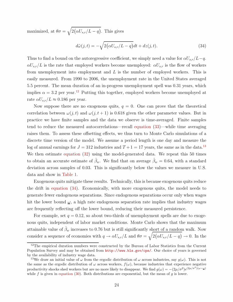
maximized, at θσ =√

2(

αUs,r/L − q)

. This gives

dω(j, t) = −√

2(

αUs,r/L − q)

dt + dz(j, t). (34)

Thus to find a bound on the autoregressive coefficient, we simply need a value for αUs,r/L−q.

αUs,r/L is the rate that employed workers become unemployed: αUs,r is the flow of workers

from unemployment into employment and L is the number of employed workers. This is

easily measured. From 1990 to 2006, the unemployment rate in the United States averaged

5.5 percent. The mean duration of an in-progress unemployment spell was 0.31 years, which

implies α = 3.2 per year.12 Putting this together, employed workers become unemployed at

rate αUs,r/L ≈ 0.186 per year.

Now suppose there are no exogenous quits, q = 0. One can prove that the theoretical

correlation between ω(j, t) and ω(j, t + 1) is 0.618 given the other parameter values. But in

practice we have finite samples and the data we observe is time-averaged. Finite samples

tend to reduce the measured autocorrelations—recall equation (33)—while time averaging

raises them. To assess these offsetting effects, we thus turn to Monte Carlo simulations of a

discrete time version of the model. We assume a period length is one day and measure the

log of annual earnings for J = 312 industries and T +1 = 17 years, the same as in the data.13

We then estimate equation (32) using the model-generated data. We repeat this 50 times

to obtain an accurate estimate of βw. We find that on average βw = 0.64, with a standard

deviation across samples of 0.03. This is significantly below the values we measure in U.S.

data and show in Table 1.

Exogenous quits mitigate these results. Technically, this is because exogenous quits reduce

the drift in equation (34). Economically, with more exogenous quits, the model needs to

generate fewer endogenous separations. Since endogenous separations occur only when wages

hit the lower bound ω, a high rate endogenous separation rate implies that industry wages

are frequently reflecting off the lower bound, reducing their measured persistence.

For example, set q = 0.12, so about two-thirds of unemployment spells are due to exoge-

nous quits, independent of labor market conditions. Monte Carlo shows that the maximum

attainable value of βw increases to 0.76 but is still significantly short of a random walk. Now

consider a sequence of economies with q → αUs,r/L and θσ =√

2(

αUs,r/L − q)

→ 0. In the

12The empirical duration numbers were constructed by the Bureau of Labor Statistics from the CurrentPopulation Survey and may be obtained from http://www.bls.gov/cps/. Our choice of years is governedby the availability of industry wage data.

13We draw an initial value of ω from the ergodic distribution of ω across industries, say g(ω). This is notthe same as the ergodic distribution of ω across workers, f(ω), because industries that experience negative

productivity shocks shed workers but are no more likely to disappear. We find g(ω) = −(2µ/σ2)e(2µ/σ2)(ω−ω)

while f is given in equation (30). Both distributions are exponential, but the mean of g is lower.

24

limit, ω follows a random walk and so the estimated value of βw converges to T−2T+1

= 0.82.

While this is arguably close to the empirical value of 0.91, the model is not very interesting.

Unemployed workers find jobs at rate α and lose them at rate q, both exogenous parameters.

The variance in wages is infinitely large and wages are perfectly persistent and so unregulated

by the entry and exit of workers. In other words, the equilibrating mechanism in Lucas and

Prescott (1974) is shut down.

6.3 Directed Search Model without Rest Unemployment

Our analysis of the directed search model in Section 4 is similar. We still assume that

productivity drift satisfies µx = −12(θ− 1)σ2

x and focus on the limit as δ → 0. We again shut

down rest unemployment, br = 0.

In the directed search model, wages are a Brownian motion dω(j, t) = µdt + σdz(j, t),

regulated on [ω, ω]. Using equation (13), our assumption on the relationship between the

drift and standard deviation of productivity implies a similar relationship for wages,

µ = −12θσ2 +

q

θ.

In this case, the estimated autoregressive coefficient depends on αUs/L, q, and θσ. To prove

this, again let ω(j, t) = (ω(j, t)−ω)/σ. This has the same autoregressive coefficient βw as ω,

but satisfies a simpler law of motion,

dω(j, t) =(

−12θσ +

q

θσ

)

dt + dz, (35)

for ω(j, t) ∈ [0, (ω − ω)/σ]. Invert equation (18) to express this interval as

ω(j, t) ∈[

0,−θσ

2qlog

(

1 − qL

αUs

)]

.

In the random search case, the autoregressive coefficient depended only on the difference

αUs/L − q, while here the two objects enter separately. Still, the spirit of our previous

analysis carries over to this case. In particular, for fixed αUs/L and q, the autoregressive

coefficient is a nonmonotonic function of θσ. When θσ is close to zero, ω lies in a small

interval and so is nearly serially uncorrelated. When θσ is large, ω has a strong negative

drift. As in the random search model, this again eliminates the serial correlation. The

estimated autoregressive coefficient is therefore maximized at an intermediate value of θσ,

although unlike in the random search model, we do not have an explicit expression for the

maximizing value, but rather proceed using Monte Carlo.

25

Again fix αUs/L ≈ 0.186 per year and initially assume q = 0; note that in this limit, the

upper bound on ω converges to θσ2αUs/L

. Our Monte Carlo simulations indicate a maximum

value of βw ≈ 0.56 when θσ = 1.3. Introducing exogenous quits again mitigates but does not

eliminate these issues; the economic intuition is unchanged from the random search model.

With q = 0.12, we find that the maximum value of βw increases to 0.71, attained when

θσ ≈ 1.2. Both of these autoregressive coefficients are somewhat smaller than in the random

search model. The limit as q → αUs/L is actually unchanged from the random search

model—an appropriate choice of θσ implies wages a random walk and so the estimated value

of βw converges to T−2T+1

≈ 0.82.14 Once again, we do find this limit particularly interesting.

6.4 Rest Unemployment

If some unemployment is accounted for by workers waiting for labor market conditions to

improve, our model generates more persistent fluctuations in wages. This happens for two

reasons. First, the arguments behind equations (34) and (35) suggest that if the search un-

employment rate is lower, the maximum possible autocorrelation in the log full-employment

wage ω is higher. Second, we measure the actual wage, not the full-employment wage, in the

data. Rest unemployment imposes a lower bound on wages, which further increases their

persistence.

To evaluate the quantitative importance of these effects, we calibrate the model. The

first critical issue is the empirical counterpart of search and rest unemployment. We refer

to the evidence on “stayers” and “switchers” developed by Murphy and Topel (1987) from

the March Current Population Survey and by Loungani and Rogerson (1989) from the Panel

Study of Income Dynamics (PSID). These papers classify unemployed workers as stayers if

they remain in the same two-digit industry after an unemployment spell and as switchers

otherwise. Despite differences in their data sources and methodology, both papers find that

workers switch industries after about one quarter of all unemployment spells and otherwise

return their old industry. Moreover, Loungani and Rogerson (1989) report that switchers

account for about a third of all weeks of unemployment, i.e. they stay unemployed slightly

longer than stayers.

To map this into our model, we assume that a labor market is the theoretical counterpart

of an industry in Murphy and Topel (1987) and Loungani and Rogerson (1989). Then

according to our model, all stayers must have experienced a spell of rest unemployment,

14For fixed q, let θσ =√

2q, so ω(j, t) has no drift. In the ergodic distribution, ω(j, t) is uniformlydistributed on

[

0,−√2q log

(

1 − qL/αUs

)]

. Ball and Roma (1998) prove that the autocorrelation of wagesdepends only on the width of this interval. In particular, in the limit as q → αUs/L, the upper bound on theinterval converges to infinity and wages follow a random walk.

26

q θσ βw (s.d.) σw/σ (s.d.) θ br/bi κ0 0.29 0.82 (0.01) 0.49 (0.01) 4.3 0.96 1.80.02 0.23 0.84 (0.01) 0.51 (0.01) 3.6 0.96 3.4

random search0.03 0.11 0.85 (0.01) 0.50 (0.01) 1.7 0.97 2.40.04 0.06 0.87 (0.01) 0.53 (0.02) 0.96 0.99 520 0.64 0.79 (0.01) 0.46 (0.01) 8.9 0.96 2.90.02 0.52 0.82 (0.01) 0.48 (0.01) 7.6 0.96 3.2

directed search0.03 0.49 0.84 (0.01) 0.46 (0.01) 6.8 0.97 4.70.04 0.44 0.85 (0.02) 0.37 (0.02) 4.9 0.99 13

Table 2: Results from random and directed search models with 1.3% search unemployment,4.2% rest unemployment, and α = 3.2. Each row shows a different value of the exogenous quitrate q (first column) and the value of θσ (second column) that maximizes the autoregressivecoefficient βw (third column). The fourth column shows the standard deviation of the residualfrom estimating equation (33), which is proportional to σ. The numbers in parenthesis inthe third and fourth columns are the standard deviation of the estimates of βw and σw acrossruns of the model. The fifth column shows the value of θ such that σw ≈ 0.033. The last twocolumns impose ρ = 0.05 and show the implied structural parameters br/bi and κ.

while switchers’ unemployment spell ended with search but may have also included some

rest unemployment. Thus the share of rest unemployment in the overall unemployment rate

should be slightly larger than Loungani and Rogerson’s (1989) two-third share of stayers.

This motivates our targets for the search unemployment rate, Us/(Us + L) = 0.013, and for

the rest unemployment rate Ur/(Ur + L) = 0.042, totalling the same 5.5% unemployment

rate as before. We keep the arrival rate of job offers to searchers fixed at α = 3.2.

We again simulate finite panels using our model and estimate the autoregressive coefficient

βw using equation (33). As in the model without rest unemployment, we find that βw

is a nonmonotonic function of θσ. Table 2 reports the value of θσ that maximizes the

average measured autoregressive coefficient βw for different values of the exogenous quit rate

q and for both random and directed search. Note that the structure of our model imposes

q ≤ αUs/L ≈ 0.042.

Two patterns emerge from this table, both consistent with the models without rest un-

employment: higher values of q imply more persistence in wages; and a given value of q, the

directed search model generates slightly less persistent wages than the random search model.

But rest unemployment significantly raises the measured persistence of wages. Recall that

with only search unemployment, we found that the autoregressive coefficient was bounded

above by βw = T−2T+1

= 0.82 and we only obtained that bound in the limit when all unem-

ployment was due to exogenous quits. With rest unemployment, the random search model

exceeds that bound for almost any value of q, while the directed search model exceeds it if

27

q > 0.02. Although the empirical counterpart of this object is around 0.9, rest unemployment

helps close the gap between model and data.

6.5 Structural Parameters

We now return to our structural model and look at how preference parameters affect the

measured persistence of wages. We consider both the random and directed search models.

We assume throughout that the search unemployment rate is Us/(Us + L) = 0.013 and the

rest unemployment rate is Ur/(Ur + L) = 0.042. The search unemployed find jobs at rate

α = 3.2. For a given value of the exogenous quit rate q, we set θσ so as to maximize the

autoregressive coefficient in wages, i.e. at the values in Table 2.

To determine θ and σ separately, we use evidence on the estimated standard error of the

residual in equation (33), given in the fourth column of Table 2. According to our model, this

is proportional to the standard deviation of wages σ, while the data in Table 1 indicate that

σw ≈ 0.033 at the five-digit level. The fifth column shows the implied value of the elasticity

of substitution θ, which varies from slightly less than 1 to almost 9, depending on the choice

of q and whether search is random or directed. Evidence in Broda and Weinstein (2006) gives

us a sense that the middle of this range may be reasonable. They estimate the elasticity of

substitution between goods at the five-digit SITC level using international trade data, and

report a median elasticity of 2.8 (see their Table IV).15

We again start with the random search model. Equation (27) implies that search un-

employed workers arrive in labor markets at rate s = 0.042. Then equations (29) and (31)

determine ω − ω, 0.08 with q = 0 and 0.31 with q = 0.04. Next, building on our analysis of

the value function in Appendix A.8, we use equations (8) and (20) to pin down the relative

leisure values of rest unemployment and inactivity,

br

bi=

ζ2 − 1

ζ2 − 1 + e−ζ2(ω−ω),

where ζ2 is the larger root of equation (61). With q = 0, we find br/bi = 0.96, while q = 0.04

requires a higher relative value of rest unemployment, br/bi = 0.99. More generally, in order

to generate rest unemployment, br/bi must exceed 1− 1/ζ2, which is 0.91 without exogenous

quits and 0.87 with q = 0.04. This suggests that, while the rest unemployed must pay some

15This elasticity is in line with the one used in much of the literature that quantitatively evaluates theLucas and Prescott (1974) model. Recall that the analog of θ in a model with diminishing returns at thelabor market level due to a fixed factor is the reciprocal of the elasticity of revenue with respect to the fixedfactor. If the fixed factor is capital, then a capital share of 1

3 is empirically reasonable. Alvarez and Veracierto(1999) set the elasticity of fixed factor to 0.36, Alvarez and Veracierto (2001) set it to 0.23, and Kambourovand Manovskii (2007) set it to 0.32, in line with values of θ between 2.8 and 4.3.

28

cost to remain in contact with their labor market, the cost is small. Rest unemployment

and inactivity may look quite similar to an outsider who observes individuals’ time use, even

though the rest unemployed are much more likely to return to work.

Next we consider the search cost κ = (v− v)/bi. We find this by computing the expected

value of finding a new labor market from equation (22). With q = 0, we obtain κ = 1.8,

while q = 0.04 requires a much higher value, κ = 52.16 In words, the expected cost of moving

to a new market must be equal to 1.8 years of inactivity in the model without exogenous

quits, and much higher with a high exogenous quit rate. A strong autocorrelation in wages

requires that most markets are far from the lower threshold ω, but this implies that the wage

in an average market is much higher than the wage in the least productive market. In order

for workers to be willing to endure such a market, the cost of moving must be large. This is

essentially the contrapositive of Hornstein, Krusell, and Violante’s (2006) finding that when

search costs are small, search models cannot generate much wage dispersion. Introducing

other mobility costs, such as market-specific human capital, may alleviate this issue.

The determination of the structural parameters in the directed search model is similar.

We first use the expression for the search unemployment rate in equation (18) to pin down

ω − ω, 0.55 with q = 0 and 1.47 with q = 0.04. We then use the equation for the rest

unemployment rate to find ω − ω, 0.08 without quits and 0.45 with the high quit rate.

Finally, equation (12) gives us the remaining parameters. Without quits, we get br/bi = 0.96

and κ = 2.9. With q = 0.04, both numbers are larger, br/bi = 0.99 and κ = 13. These

numbers are comparable to the ones in the random search model, and the intuition is simlar.

We have focused here on the relative leisure values from search unemployment, rest un-

employment, and inactivity. To do this, we did not need to take a stand on the utility

function. For the model to be consistent with balanced growth, we would additionally re-

quire u(·) = log(·). In this case, data on labor force participation rates would pin down the

absolute level of the three leisure parameters.

Finally, it is worth stressing that these high values of search costs κ are a consequence

of persistent wages and not due to rest unemployment per se. Suppose we shut down rest

unemployment but let q → αUs/L so that wages are nearly a random walk, regardless of

whether search is random or directed. In either case, the incentive to search for a job is large

and so search costs must be large in equilibrium as well, reaching infinity in the limit when

wages a random walk. For example, with a 5.5 percent search unemployment rate and no

rest unemployment, αUs/L = 0.186. Set q = 0.18 to generate βw = 0.85 and σw = 0.70 in

the random search model. These reduced form parameters imply θ = 2.4, br/bi = 0.94, and

16An increase in θ raises br/bi and reduces κ. Indeed, part of the reason that the implied search costs areso high when q = 0.04 is because θ is so small. With q = 0.04 and θ = 4.3, we obtain br/bi = 0.972 andκ = 2.25; however, the model then generates too little wage volatility.

29

κ = 2.6, comparable to values in the full model with rest unemployment.

7 Concluding Remarks

This paper characterizes the equilibrium of the Lucas-Prescott search model with directed

and random search. Our characterization features a separation between optimization and

aggregation which keeps our analysis tractable. We use this separation to argue that we can

distinguish economies between economies with different amounts of search and rest unem-

ployment, arguing that rest unemployment helps to explain why wages are so persistent yet

unemployment incidence is high.

Although our’s is the first paper to separate optimization from aggregation in the context

of the Lucas and Prescott (1974) search model, others have fruitfully used the same idea in

different contexts. Caballero and Engel (1993) evaluate the magnitude and effect of labor

adjustment costs by looking at the statistical behavior of employment at the firm level. Doms

and Dunne (1998) perform a similar exercise for capital adjustment costs and irreversibilities.

Cole and Rogerson (1999) examine whether the Mortensen and Pissarides (1994) model is

consistent with the behavior of job creation and destruction at business cycle frequencies by

using a reduced-form version of the original model. Hall (1995) similarly studies the propa-

gation of one-time shocks in an elaboration of this model through a statistical representation

of the labor market as a 19-state Markov process.

One important question is the empirical counterpart of rest unemployment. We used

evidence on whether workers switch industries after a spell of unemployment to pin down

the rest unemployment rate, but a more direct link may be desirable. Workers on temporary

layoff are an obvious example of rest unemployment, since they are waiting for conditions

in the industry to improve. Interestingly, Katz and Meyer (1990) and Starr-McCluer (1993)

find that the hazard rates of workers on temporary layoff are more strongly decreasing as a

function of unemployment duration, compared to other unemployed workers. While the cur-

rent version of the model does not have an explicit characterization unemployment duration,

our extension in Alvarez and Shimer (2009) does. We develop a version of this model where

unions can keep wages above the market-clearing level and allocate jobs based on seniority.

We show that the hazard rate of reentering unemployed is decreasing in duration for workers

who are rationed out of jobs. Moreover, we think that in that version of the model, the iden-

tification of the rest unemployed as workers on temporary layoff is quite descriptive. While

the determination of the thresholds ω and ω is more complicated in that framework, the

same separation between optimization and aggregation applies and the link between search

unemployment rates and wages is unchanged.

30

A Appendix

A.1 Density of Productivity x

Let fx(x) denote the steady state density of log productivity, x ≡ log x, across labor markets.

This solves a Kolmogorov forward equation:

δfx(x) = −µxf′x(x) +

σ2x

2f ′′

x (x)

at all x 6= x0 ≡ log x0. The solution to this equation takes the form

fx(x) =

D11e

η1x + D12e

η2x if x < log x0

D21e

η1x + D22e

η2x if x > log x0,

where η1 < 0 < η2 are the two real roots of the characteristic equation

δ = −µxη +σ2

x

2η2. (36)

For this to be a well-defined density, integrating to 1 on (−∞,∞), we require that D11 =

D22 = 0. To pin down the remaining constants, we use two more conditions: the density is

continuous at x = log x0; and it integrates to 1. Imposing these boundary conditions delivers

fx(x) =

η1η2

η1−η2eη2(x−log x0) if x < log x0

η1η2

η1−η2eη1(x−log x0) if x > log x0.

(37)

With this notation, we obtain

(∫ 1

0

x(j, t)θ−1dj

)

1θ−1

=

(∫ ∞

−∞

e(θ−1)xfx(x)dx

)1

θ−1

. (38)

The interior integral converges if η1 + θ − 1 < 0 < η2 + θ − 1. The definition of ηi in

equation (36) implies these inequalities are equivalent to condition (6). With this restriction,

we can then simplify equation (38) to obtain equation (7).

A.2 Proof of Proposition 1

Throughout this proof we express the value of a worker v as a function not only on the

current log wage ω but also of the lower and upper bound on wages ω and ω, say v(ω; ω, ω).

We start by proving a preliminary result.

31

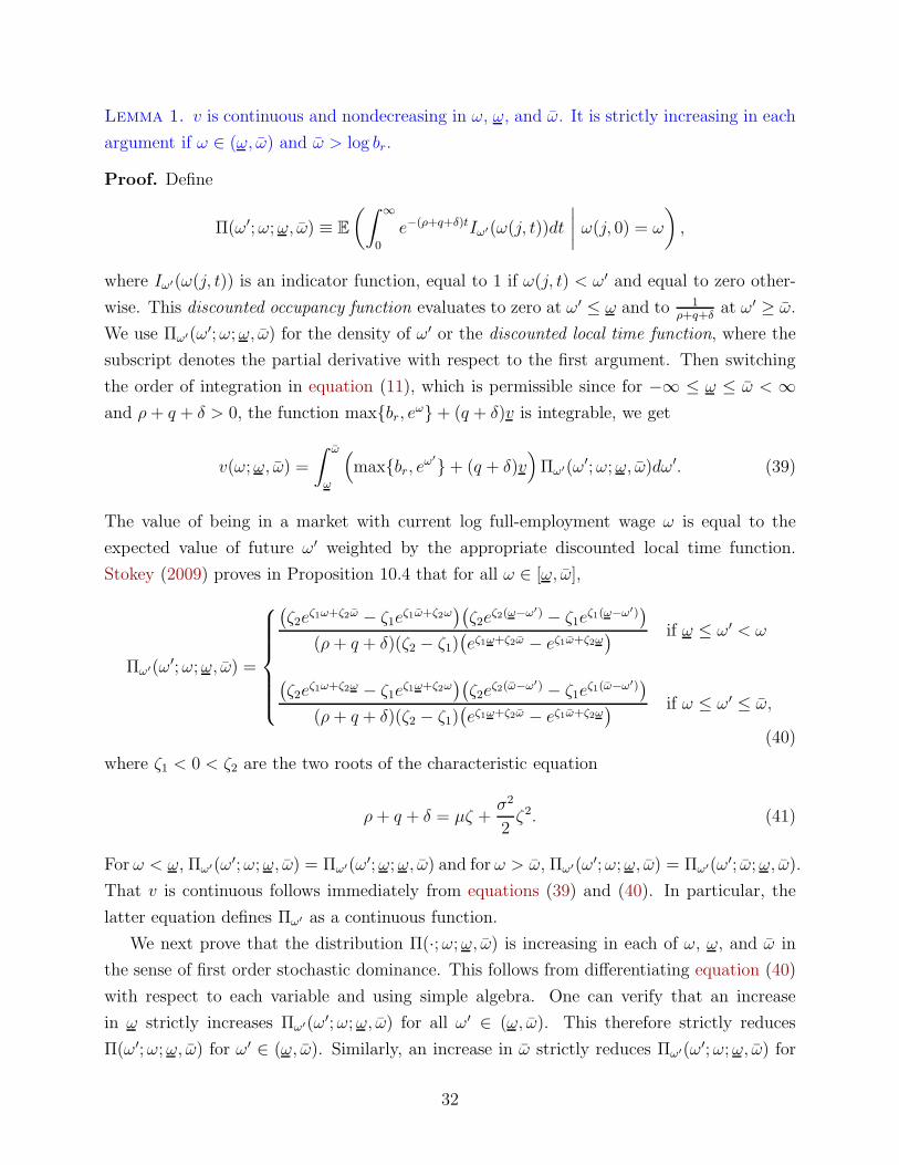
Lemma 1. v is continuous and nondecreasing in ω, ω, and ω. It is strictly increasing in each

argument if ω ∈ (ω, ω) and ω > log br.

Proof. Define

Π(ω′; ω; ω, ω) ≡ E

(∫ ∞

0

e−(ρ+q+δ)tIω′(ω(j, t))dt

∣

∣

∣

∣

ω(j, 0) = ω

)

,

where Iω′(ω(j, t)) is an indicator function, equal to 1 if ω(j, t) < ω′ and equal to zero other-

wise. This discounted occupancy function evaluates to zero at ω′ ≤ ω and to 1ρ+q+δ

at ω′ ≥ ω.

We use Πω′(ω′; ω; ω, ω) for the density of ω′ or the discounted local time function, where the

subscript denotes the partial derivative with respect to the first argument. Then switching

the order of integration in equation (11), which is permissible since for −∞ ≤ ω ≤ ω < ∞and ρ + q + δ > 0, the function maxbr, e

ω + (q + δ)v is integrable, we get

v(ω; ω, ω) =

∫ ω

ω

(

maxbr, eω′ + (q + δ)v

)

Πω′(ω′; ω; ω, ω)dω′. (39)

The value of being in a market with current log full-employment wage ω is equal to the

expected value of future ω′ weighted by the appropriate discounted local time function.

Stokey (2009) proves in Proposition 10.4 that for all ω ∈ [ω, ω],

Πω′(ω′; ω; ω, ω) =

(

ζ2eζ1ω+ζ2ω − ζ1e

ζ1ω+ζ2ω)(

ζ2eζ2(ω−ω′) − ζ1e

ζ1(ω−ω′))

(ρ + q + δ)(ζ2 − ζ1)(

eζ1ω+ζ2ω − eζ1ω+ζ2ω) if ω ≤ ω′ < ω

(

ζ2eζ1ω+ζ2ω − ζ1e

ζ1ω+ζ2ω)(

ζ2eζ2(ω−ω′) − ζ1e

ζ1(ω−ω′))

(ρ + q + δ)(ζ2 − ζ1)(

eζ1ω+ζ2ω − eζ1ω+ζ2ω) if ω ≤ ω′ ≤ ω,

(40)

where ζ1 < 0 < ζ2 are the two roots of the characteristic equation

ρ + q + δ = µζ +σ2

2ζ2. (41)

For ω < ω, Πω′(ω′; ω; ω, ω) = Πω′(ω′; ω; ω, ω) and for ω > ω, Πω′(ω′; ω; ω, ω) = Πω′(ω′; ω; ω, ω).

That v is continuous follows immediately from equations (39) and (40). In particular, the

latter equation defines Πω′ as a continuous function.

We next prove that the distribution Π(·; ω; ω, ω) is increasing in each of ω, ω, and ω in

the sense of first order stochastic dominance. This follows from differentiating equation (40)

with respect to each variable and using simple algebra. One can verify that an increase

in ω strictly increases Πω′(ω′; ω; ω, ω) for all ω′ ∈ (ω, ω). This therefore strictly reduces

Π(ω′; ω; ω, ω) for ω′ ∈ (ω, ω). Similarly, an increase in ω strictly reduces Πω′(ω′; ω; ω, ω) for

32

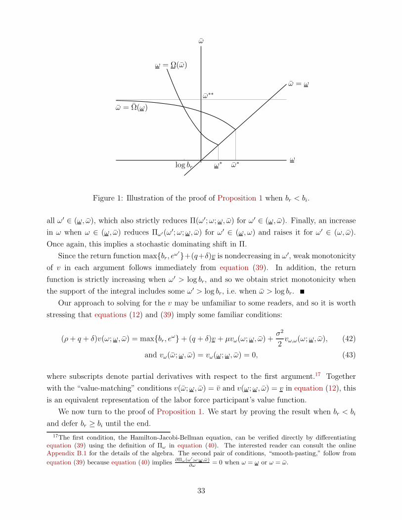
ω

ω

log br

ω = ω

ω∗ω∗

ω∗∗

ω = Ω(ω)

ω = Ω(ω)

Figure 1: Illustration of the proof of Proposition 1 when br < bi.

all ω′ ∈ (ω, ω), which also strictly reduces Π(ω′; ω; ω, ω) for ω′ ∈ (ω, ω). Finally, an increase

in ω when ω ∈ (ω, ω) reduces Πω′(ω′; ω; ω, ω) for ω′ ∈ (ω, ω) and raises it for ω′ ∈ (ω, ω).

Once again, this implies a stochastic dominating shift in Π.

Since the return function maxbr, eω′+(q+δ)v is nondecreasing in ω′, weak monotonicity

of v in each argument follows immediately from equation (39). In addition, the return

function is strictly increasing when ω′ > log br, and so we obtain strict monotonicity when

the support of the integral includes some ω′ > log br, i.e. when ω > log br.

Our approach to solving for the v may be unfamiliar to some readers, and so it is worth

stressing that equations (12) and (39) imply some familiar conditions:

(ρ + q + δ)v(ω; ω, ω) = maxbr, eω + (q + δ)v + µvω(ω; ω, ω) +

σ2

2vω,ω(ω; ω, ω), (42)

and vω(ω; ω, ω) = vω(ω; ω, ω) = 0, (43)

where subscripts denote partial derivatives with respect to the first argument.17 Together

with the “value-matching” conditions v(ω; ω, ω) = v and v(ω; ω, ω) = v in equation (12), this

is an equivalent representation of the labor force participant’s value function.

We now turn to the proof of Proposition 1. We start by proving the result when br < bi

and defer br ≥ bi until the end.

17The first condition, the Hamilton-Jacobi-Bellman equation, can be verified directly by differentiatingequation (39) using the definition of Πω in equation (40). The interested reader can consult the onlineAppendix B.1 for the details of the algebra. The second pair of conditions, “smooth-pasting,” follow from

equation (39) because equation (40) implies∂Πω(ω′;ω;ω,ω)

∂ω = 0 when ω = ω or ω = ω.

33

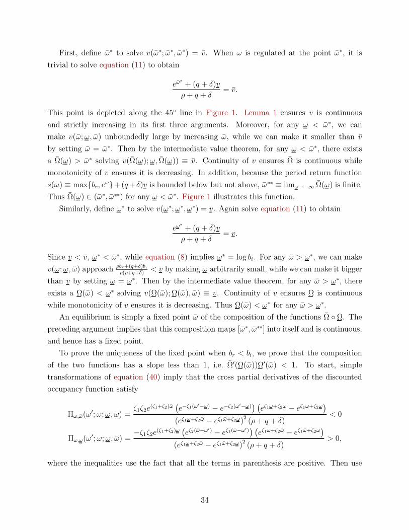
First, define ω∗ to solve v(ω∗; ω∗, ω∗) = v. When ω is regulated at the point ω∗, it is

trivial to solve equation (11) to obtain

eω∗

+ (q + δ)v

ρ + q + δ= v.

This point is depicted along the 45 line in Figure 1. Lemma 1 ensures v is continuous

and strictly increasing in its first three arguments. Moreover, for any ω < ω∗, we can

make v(ω; ω, ω) unboundedly large by increasing ω, while we can make it smaller than v

by setting ω = ω∗. Then by the intermediate value theorem, for any ω < ω∗, there exists

a Ω(ω) > ω∗ solving v(Ω(ω); ω, Ω(ω)) ≡ v. Continuity of v ensures Ω is continuous while

monotonicity of v ensures it is decreasing. In addition, because the period return function

s(ω) ≡ maxbr, eω+(q+ δ)v is bounded below but not above, ω∗∗ ≡ limω→−∞ Ω(ω) is finite.

Thus Ω(ω) ∈ (ω∗, ω∗∗) for any ω < ω∗. Figure 1 illustrates this function.

Similarly, define ω∗ to solve v(ω∗; ω∗, ω∗) = v. Again solve equation (11) to obtain

eω∗

+ (q + δ)v

ρ + q + δ= v.

Since v < v, ω∗ < ω∗, while equation (8) implies ω∗ = log bi. For any ω > ω∗, we can make

v(ω; ω, ω) approach ρbr+(q+δ)bi

ρ(ρ+q+δ)< v by making ω arbitrarily small, while we can make it bigger

than v by setting ω = ω∗. Then by the intermediate value theorem, for any ω > ω∗, there

exists a Ω(ω) < ω∗ solving v(Ω(ω); Ω(ω), ω) ≡ v. Continuity of v ensures Ω is continuous

while monotonicity of v ensures it is decreasing. Thus Ω(ω) < ω∗ for any ω > ω∗.

An equilibrium is simply a fixed point ω of the composition of the functions Ω Ω. The

preceding argument implies that this composition maps [ω∗, ω∗∗] into itself and is continuous,

and hence has a fixed point.

To prove the uniqueness of the fixed point when br < bi, we prove that the composition

of the two functions has a slope less than 1, i.e. Ω′(Ω(ω))Ω′(ω) < 1. To start, simple

transformations of equation (40) imply that the cross partial derivatives of the discounted

occupancy function satisfy

Πω,ω(ω′; ω; ω, ω) =ζ1ζ2e

(ζ1+ζ2)ω(

e−ζ1(ω′−ω) − e−ζ2(ω′−ω)) (

eζ1ω+ζ2ω − eζ1ω+ζ2ω)

(eζ1ω+ζ2ω − eζ1ω+ζ2ω)2(ρ + q + δ)

< 0

Πω,ω(ω′; ω; ω, ω) =−ζ1ζ2e

(ζ1+ζ2)ω(

eζ2(ω−ω′) − eζ1(ω−ω′)) (

eζ1ω+ζ2ω − eζ1ω+ζ2ω)

(eζ1ω+ζ2ω − eζ1ω+ζ2ω)2(ρ + q + δ)

> 0,

where the inequalities use the fact that all the terms in parenthesis are positive. Then use

34

integration-by-parts on equation (39) to write

v(ω; ω, ω) =s(ω)

ρ + q + δ−∫ ω

ω

s′(ω′)Π(ω′; ω; ω, ω)dω′,

where the period return function s(ω′) is nondecreasing and strictly increasing for ω′ > log br,

and Π is the discounted occupancy function. Taking the cross partial derivatives of this

expression gives vω,ω(ω; ω, ω) > 0 > vω,ω(ω; ω, ω). In particular,

vω(ω; ω, ω) > vω(ω; ω, ω) and vω(ω; ω, ω) > vω(ω; ω, ω).

Now since vω(ω; ω, ω) > 0 from Lemma 1, these inequalities imply

vω(ω; ω, ω)

vω(ω; ω, ω) + vω(ω; ω, ω)

vω(ω; ω, ω)

vω(ω; ω, ω) + vω(ω; ω, ω)< 1.

In particular, this is true when evaluated at any point ω, ω where ω = Ω(ω) and ω = Ω(ω).

Implicit differentiation of the definitions of these functions shows that the first term in the

above inequality is −Ω′(ω) and the second term is −Ω′(ω), which proves Ω′(Ω(ω))Ω′(ω) < 1.

Next we prove proportionality of the thresholds eω and eω to the leisure values br, bi,

and bs. From equations (8) and (9), v and v are homogeneous of degree one in the three

leisure values. The function maxbr, eω + (q + δ)v is also homogeneous of degree 1 in the

leisure values and eω. By inspection of equation (40), Πω is unaffected by an equal absolute

increase in each of its arguments. Then the integral in equation (39) is homogeneous of

degree one in the b’s and eω and eω. The result follows from equation (12).

Finally we consider br ≥ bi, so the period return function s(ω) ≥ bi+(q+δ)v for all ω. This

implies v(ω;−∞, ω) ≥ v for all ω and ω. Then an equilibrium is defined by v(ω;−∞, ω) = v.

As discussed above, the solution of this equation is ω∗∗ ∈ (ω∗,∞).

A.3 Proof of Proposition 2

First, set br = 0. By Proposition 1, there exists a unique equilibrium characterized by

thresholds ω0 and ω0. We now prove that br ≡ eω0 . To see why, observe that for all

br ≤ br, the equations characterizing equilibrium are unchanged from the case of br = 0

because log br ≤ ω0, and hence the equilibrium is unchanged. Conversely, for all br > br, the

equations characterizing equilibrium necessarily are changed, and so the equilibrium must

have log br > ωbr.

Next we prove that br/bi = B(κ, ρ+q+δ, µ, σ). Again with br = 0, combine equations (12)

and (39), noting the discounted local time function Πω integrates to 1ρ+q+δ

, and use the

35

definitions of v and v in equations (8) and (9):

bi

ρ + q + δ=

∫ ω0

ω0

eωΠω(ω; ω0; ω0, ω0)dω and

bi

(

1

ρ + q + δ+ κ

)

=

∫ ω0

ω0

eωΠω(ω; ω0; ω0, ω0)dω.

Since Πω is homogeneous of degree zero in the exponentials of its arguments (see equation 40),

this implies eω0 and eω0 are homogeneous of degree 1 in bi. Moreover, ζi depends on ρ + q +

δ, µ, and σ by equation (41) and so the density Πω in equation (40) depends on these

same parameters. It follows that the solution to these equations can depend only on these

parameters and the parameters on the left hand side of the above equations. In particular,

this proves

eω0 = biB(κ, ρ + q + δ, µ, σ).

Since br = eω0 , that establishes the dependence of br on this limited set of parameters.

Obviously B is positive-valued. By Proposition 1, ω0 < log bi and so B < 1. We finally

prove it is decreasing in κ. Since κ affects ω and ω only through v, to establish that B is

decreasing in κ it suffices to show that the ω and ω that solve equations (12) and (39) is

decreasing in v. This follows because Ω(ω) is increasing in v and Ω(ω) is unaffected, where

these functions are defined in the proof of Proposition 1. A decrease in v then reduces the

composition Ω Ω. Since the slope of this function is less than 1, it reduces the location of

the fixed point ω and hence raises ω = Ω(ω).

A.4 Proof of Proposition 3

We start by characterizing the stationary distribution of workers across log full-employment

wages ω, f , defined on [ω, ω]. Since f is a density,

∫ ω

ω

f(ω)dω = 1. (44)

By taking the limit of a discrete time, discrete state-space analog of our model, we prove in

Appendix A.5 that this density has to satisfy three conditions, equations (45)–(47) below.

First, in the interior of its support, it must solve a Kolmogorov forward equation,

(q + δ)f(ω) = −µf ′(ω) +σ2

2f ′′(ω) for all ω ∈ (ω, ω). (45)

36

This captures the requirement that inflows and outflows balance at each point in the support

of the density. Workers exit markets either because of quits or shutdowns at rate q + δ, while

otherwise ω is a Brownian motion with drift µ and standard deviation σ. Workers whose ω

changes leave this point in the density for higher or lower values of ω, while the density picks

up mass from points above and below when they are hit by appropriate shocks. In a short

period of time, this relates the density of f at nearby points, i.e. it relates the level of f and

its derivatives.

Second, at the lower bound ω,

σ2

2f ′(ω) −

(

µ +θσ2

2

)

f(ω) = 0. (46)

The elasticity of substitution θ appears in this equation because it determines how many

workers must exit from depressed markets required to regulate ω above ω. The exogenous

separation rate q + δ does not appear in this equation because the ratio of endogenous to

exogenous exits is infinite in a short time interval for a market at the lower bound. Since by

definition there are no markets with smaller ω, f(ω) is not fed from below, which explains

the difference between equations (45) and (46). The second order differential equation (45)

and the boundary conditions equations (44) and (46) yield equation (14) using standard

calculations.

We now turn to output and consumption (which are equal by the final goods market

clearing condition) and employment. Appendix A.5 also establishes that at the upper bound

ω,σ2

2f ′(ω) −

(

µ +θσ2

2

)

f(ω) = δL0

L, (47)

where L0 is the (endogenous) average number of workers in a new labor market. The logic

for the left hand side of this equation parallels the logic behind equation (46). There is an

extra inflow at ω coming from newly-formed markets, which absorb δL0 workers per unit

of time; dividing by L expresses this inflow as a percentage of the workers located in labor

markets.

Next, equation (5) implies that the number of workers in a new labor market is

L0 = Y u′(Y )θxθ−10 e−θω, (48)

which ensure a log full-employment wage ω.

Our last condition relates intermediate and final goods output. It is convenient to first

define the productivity of a location x consistent with l workers present in the location, a log

full-employment wage ω, and aggregate output and consumption Y . From equation (5), this

37

solves

x = ξ(l, ω, Y ) ≡(

leθω

Y u′(Y )θ

)1

θ−1

. (49)

Use this to compute output in a market with l workers and log full-employment wage ω,

recognizing that there may be rest unemployment:

Q(l, ξ(l, ω, Y )) = Y−1θ−1

(

eωl

u′(Y )

) θθ−1

min1, eω/brθ. (50)

Using this notation, we can write equation (2) as

Y =

(∫ 1

0

Q(

l(j, t), ξ(l(j, t), ω(j, t), Y ))

θ−1θ dj

)θ

θ−1

(51)

=

(∫ 1

0

Q(

L, ξ(L, ω(j, t), Y ))

θ−1θ

l(j, t)

Ldj

)

θθ−1

Note that these equations have to hold for all t in steady state, so the choice of t is arbitrary.

The second equation follows because Q(·, ξ(·, ω, Y ))θ−1

θ is linear (equation 50). To solve this,

we change the variable of integration from the name of the market j to its log full-employment

wage ω and number of workers l. Let f(ω, l) be the ergodic density of the joint distribution

of workers in markets (ω, l). The joint distribution of (ω, l) for an individual worker is a

strongly convergent Markov process whenever markets shut down at a positive rate, δ > 0,

which ensures that f is unique. Without characterizing the distribution explicitly, we have

Y =

∫ ω

ω

∫ ∞

0

Q(L, ξ(L, ω, Y ))θ−1

θl

Lf(ω, l) dl dω.

Since f(ω) =∫∞

0lLf(ω, l) dl, we can solve the inner integral to obtain

Y =

(

∫ ω

ω

Q(

L, ξ(L, ω, Y ))

θ−1θ f(ω)dω

)θ

θ−1

. (52)

This depends on the known density f rather than the more complicated density f .

Finally, we solve equations (47), (48), and (52) for L0, L, and Y . First eliminate L0

between equations (47) and (48) and evaluate f(ω) using equation (14) to get

L =−2δY u′(Y )θxθ−1

0 e−θω

σ2(θ + η1)(θ + η2)(

eη2(ω−ω) − eη1(ω−ω))

2∑

i=1

|θ + ηi|eηi(ω−ω) − 1

ηi

. (53)

38

Substitute equation (50) into equation (52) to get

Y =L

u′(Y )

∫ ω

ω

eω min1, eω/brθ−1f(ω)dω

=Leω

u′(Y )

∑2i=1 |θ + ηi|e−(ω−ω)

(

eηi(ω−ω)−e−θ(ω−ω)

θ+ηi+ eηi(ω−ω) e(ω−ω)−e−ηi(ω−ω)

1+ηi

)

∑2i=1 |θ + ηi| e

ηi(ω−ω)−1ηi

, (54)

where we solve the integral using the expression for f in equation (14) and define ω ≡maxω, log br. Eliminating L between these equations and solving for u′(Y ) gives an implicit

equation for output:

u′(Y )1−θ =−2δxθ−1

0 e−(θω−ω)

σ2(θ + η1)(θ + η2)(

eη2(ω−ω) − eη1(ω−ω))×

2∑

i=1

|θ + ηi|(

eηi(ω−ω) − e−θ(ω−ω)

θ + ηi

+ eηi(ω−ω) e(ω−ω) − e−ηi(ω−ω)

1 + ηi

)

. (55)

Finally, equation (54) determines the number of workers in labor markets, L.

A.5 Derivation of the Density f

We use a discrete time, discrete state space model to obtain the Kolmogorov forward equa-

tions and boundary conditions for the density f . Divide [ω, ω] into n intervals of length

∆ω = (ω − ω)/n. Let the time period be ∆t = (∆ω/σ)2 and assume that when ω < ω, it

decreases with probability 12(1 + ∆p) where ∆p = µ∆ω/σ2; when ω > ω, it increases with

probability 12(1 − ∆p); and otherwise ω stays constant. Note that for ω < ω(t) < ω, the

expected value of ω(t + ∆t) − ω(t) is µ∆t and the second moment is σ2∆t. As n goes to

infinity, this converges to a regulated Brownian motion with drift µ and standard deviation σ.

Now let fn(ω, t) denote the fraction of workers in markets with log full employment

wage ω at time t for fixed n. With a slight abuse of notation, let fn(ω) be the stationary

distribution. We are interested in characterizing the density f(ω) = limn→∞fn(ω)∆ω

. For

ω ∈ [ω + ∆ω, ω − ∆ω], the dynamics of ω imply

fn(ω, t + ∆t) = (1 − (q + δ)∆t)(

12(1 + ∆p)fn(ω − ∆ω, t) + 1

2(1 − ∆p)fn(ω + ∆ω, t)

)

. (56)

In any period of length ∆t, a fraction (q+δ)∆t of workers leave due to market shut downs and

idiosyncratic quits. Thus the workers in markets with ω at t+∆t are a fraction 1− (q + δ)∆t

of those who were in markets at ω − ∆ω at t and had a positive shock, plus the same

fraction of those who were in markets at ω +∆ω at t and had a negative shock. Now impose

39

stationarity on fn. Take a second order approximation to fn(ω+∆ω) and fn(ω−∆ω) around

ω, substituting ∆t and ∆p by the expressions above:

fn(ω) =

(

1 − (q + δ)∆ω2

σ2

)(

fn(ω) − µ∆ω2

σ2f ′

n(ω) +∆ω2

2f ′′

n(ω)

)

⇒ (q + δ)fn(ω) =

(

1 − (q + δ)∆ω2

σ2

)(

−µf ′n(ω) +

σ2

2f ′′

n(ω)

)

Taking the limit as n converges to infinity, fn(ω)∆ω

→ f(ω) solving equation (45).

Now consider the behavior of fn at the lower threshold ω. A similar logic implies

fn(ω, t + ∆t) = (1 − (q + δ)∆t)12(1 − ∆p)

(

fn(ω + ∆ω, t) + fn(ω, t)(1 − ∆l))

.

The workers at ω at t+∆t either were at ω+∆ω or at ω at t; in both cases, they had a negative

shock. Moreover, in the latter case, a fraction ∆l ≡ θ∆ω of the workers exited the market

to keep ω above ω. Again impose stationarity but now take a first order approximation to

fn(ω + ∆ω) at ω; the higher order terms will drop out later in any case. Replacing ∆t, ∆p,

and ∆l with the expressions described above gives

fn(ω) =

(

1 − (q + δ)∆ω2

σ2

)(

1 − µ∆ω

σ2

)(

fn(ω)

(

1 − θ∆ω

2

)

+∆ω

2f ′

n(ω)

)

Again eliminating terms in fn(ω) and taking the limit as n → ∞, we obtainfn(ω)

∆ω→ f(ω)

solving equation (46).

Now consider the behavior of fn at the upper threshold ω:

fn(ω, t + ∆t) = (1 − (q + δ)∆t)12(1 + ∆p)

(

fn(ω − ∆ω, t) + fn(ω, t)(1 + ∆l))

+ δ∆tL0/L.

Compared to the equation at the lower threshold, the only significant change is the last term,

which reflects the fact that on average a fraction L0/L workers enter at the upper threshold

when a new market is created. Recall also that markets are destroyed at rate δ per unit

of time and hence δ∆tL0/L is the fraction of workers added to the upper threshold due to

newly created markets. Impose stationarity and take limits to get

fn(ω) =

(

1 − (q + δ)∆ω2

σ2

)(

1 +µ∆ω

σ2

)(

fn(ω)

(

1 +θ∆ω

2

)

− ∆ω

2f ′

n(ω)

)

+ δ∆ω2

σ2L0/L

Eliminate terms in fn(ω) and take the limit as n → ∞ to obtain fn(ω)∆ω

→ f(ω) solving

equation (47).

40

A.6 Exit Rates from Labor Markets

A worker exits her labor market if the log full-employment wage is ω and the market is hit

by an adverse shock, if the labor market closes, or if she quits. In the discrete time, discrete

state space model, the first event hits a fraction 12∆l(1 − ∆p) of the workers who survive in

a labor market with ω = ω:

Ns∆t ≡ (1 − (q + δ)∆t)12(1 − ∆p)∆lfn(ω)L + (q + δ)∆tL

Reexpress ∆ω, ∆l, and ∆p in terms of ∆t, take the limit as n → ∞, and use fn(ω)∆ω

→ f(ω),

to get equation (16).

A.7 Density f : Random Search

Since f is a density,∫ ∞

ω

f(ω)dω = 1. (57)

By taking the limit of a discrete time, discrete state-space analog of our model, we find

that this density has to satisfy three additional conditions. First, at ω > ω, it must solve a

Kolmogorov forward equation, unchanged from equation (45) except for the effect of random

search:

(q + δ − s)f(ω) = −µf ′(ω) +σ2

2f ′′(ω) for all ω > ω. (58)

Second, at the lower bound ω, we have the same condition as in the directed search case,

equation (46). Finally, in contrast with the directed search case, there is a kink in f at the

point where new markets are created:

f ′−(ω) − f ′

+(ω) =2δL

σ2L. (59)

where L is the average number of workers in a new labor market. The derivation of this

condition, which reflects the addition of directed searchers into new markets, is standard

and hence omitted. Solving these equations and emphasizing the dependence of f on the

boundary ω and the arrival rate of new workers s, we obtain equation (24).

A.8 Proof of Proposition 5

Express the value of a worker v as a function not only on the current log wage ω but also of

the lower bound on wages ω and the arrival rate of search unemployed workers s, v(ω; ω, s).

We start by proving a preliminary result.

41

Lemma 2. v is continuous and nondecreasing in ω and continuous and nonincreasing in s.

It is strictly monotone in each argument if ω > ω.

Proof. Taking limits of equation (40), we obtain

Πω′(ω′; ω; ω, s) =

ζ2eζ1(ω−ω)

(

ζ2eζ2(ω−ω′) − ζ1e

ζ1(ω−ω′))

(ρ + q + δ)(ζ2 − ζ1)if ω ≤ ω′ < ω

ζ2eζ2(ω−ω′)

(

ζ2eζ1(ω−ω) − ζ1e

ζ2(ω−ω))

(ρ + q + δ)(ζ2 − ζ1)if ω ≤ ω′ ≤ ∞,

(60)

where ζ1 < 0 < ζ2 are the two roots of the characteristic equation

ρ + q + δ = µζ +σ2

2ζ2. (61)

Of course, µ is a decreasing function of s from equation (21). The remainder of the proof

follows the structure of the proof of Lemma 1 as is omitted.

Now rewrite equations (20) and (22) to define two implicit functions of s:

v(ω1(s); ω1(s), s) = v, (62)∫ ∞

ω2(s)

v(ω; ω2(s), s)f(ω; ω2(s), s)dω = v, (63)

where our notation also emphasizes the dependence of the cross-sectional density of ω on ω

and s. An equilibrium is a solution s to

ω1(s) = ω2(s). (64)

Lemma 2 and equation (30) imply that these are continuous and increasing functions of s.

We then argue that

ω2

(

q + 12θσ2)

= −∞ < ω1

(

q + 12θσ2)

and lims→∞

ω2(s) > lims→∞

ω1(s). (65)

If s ≤ q + 12θσ2, the integral on the left hand side of equation (63) does not converge for all

ω2(s), while as s → q + 12θσ2, ω2 → −∞. On the other hand, ω1 is finite for any s. At the

other end of the range, as s → ∞, the density f puts almost all its weight at ω. This implies

that the left hand side of equation (63) converges to v(ω2(∞); ω2(∞),∞). Since v > v, we

must have ω2(∞) > ω1(∞). The existence of ω solving equation (64) then follows from the

intermediate value theorem.

42

For the case where br = 0, so there is no rest unemployment, and q = 0, equations (62)

and (63) simplify further. In this case, the left hand sides of both equations are proportional

to eω, hence taking the ratio gives

v

v≡ 1 +

ρ

vκ =

η2(s)(1 + ζ1(s) + η2(s))

(1 + η2(s))(ζ1(s) + η2(s)), (66)

where the notation emphasizes that the roots ηi for f and ζi given by equation (61) are

functions of µ, which depends on s as in equation (21). In a Mathematica file available on

request, we prove that the right hand side of equation (66) converges to ∞ as s goes to its

lower bound, and it converges to 1 as s goes to ∞. Moreover, a lengthy algebraic argument

shows that this ratio is decreasing in s everywhere. Thus, since v/v ≥ 1, there is a unique

solution s∗, and hence a unique equilibrium. It is immediate that the equilibrium value of s∗

is decreasing in the search cost κ, and since ω1 is increasing, the value of ω decreases too.

References

Abel, Andrew B. and Ben S. Bernanke. 2001. Macroeconomics. Boston: Addison Wesley

Longman, 4th ed.

Abel, Andrew B. and Janice C. Eberly. 1996. “Optimal Investment with Costly Reversibility.”

The Review of Economic Studies 63 (4):581–593.

Alvarez, Fernando and Robert Shimer. 2009. “Unions and Unemployment.” University of

Chicago mimeo.

Alvarez, Fernando and Marcelo Veracierto. 1999. “Labor-Market Policies in an Equilibrium

Search Model.” NBER Macroeconomics Annual 14:265–304.

———. 2001. “Severance Payments in an Economy with Frictions.” Journal of Monetary

Economics 47 (3):477–498.

Atkeson, Andrew, Aubhik Khan, and Lee Ohanian. 1996. “Are Data on Industry Evolution

and Gross Job Turnover Relevant for Macroeconomics?” Carnegie-Rochester Conference

Series on Public Policy 44:216–250.

Ball, Clifford A. and Antonio Roma. 1998. “Detecting Mean Reversion Within Reflecting

Barriers: Application to the European Exchange Rate Mechanism.” Applied Mathematical

Finance 5 (1):1–15.

43

Bentolila, Samuel and Giuseppe Bertola. 1990. “Firing Costs and Labour Demand: How Bad

is Eurosclerosis?” The Review of Economic Studies 47 (3):381–402.

Blanchard, Olivier J. and Lawrence F. Katz. 1992. “Regional Evolutions.” Brookings Papers

on Economic Activity 23 (1992-1):1–76.

Broda, Christian and David E. Weinstein. 2006. “Globalization and the Gains from Variety.”

The Quarterly Journal of Economics 121 (2):541–585.

Burdett, Kenneth and Tara Vishwanath. 1988. “Balanced Matching and Labor Market

Equilibrium.” Journal of Political Economy 96 (5):1048–1065.

Caballero, Ricardo J and Eduardo M R A Engel. 1993. “Microeconomic Adjustment Hazards

and Aggregate Dynamics.” The Quarterly Journal of Economics 108 (2):359–83.

Caballero, Ricardo J. and Eduardo M.R.A. Engel. 1999. “Explaining Investment Dynamics

in US manufacturing: a Generalized (S, s) Approach.” Econometrica 67 (4):783–826.

Cole, Harold L. and Richard Rogerson. 1999. “Can the Mortensen-Pissarides Matching Model

Match the Business-Cycle Facts?” International Economic Review 40 (4):933–959.

Doms, Mark E. and Timothy Dunne. 1998. “Capital Adjustment Patterns in Manufacturing

Plants.” Review of Economic Dynamics 1 (2):409–429.

Fleming, Wendell H. and Mete H. Soner. 1993. Controlled Markov Processes and Viscosity

Solutions. New York, NY: Springer-Verelag.

Gouge, Randall and Ian King. 1997. “A Competitive Theory of Employment Dynamics.”

Review of Economic Studies 64 (1):1–22.

Hall, Robert. 1995. “Lost Jobs.” Brookings Papers on Economic Activity 1:221–273.

Hamilton, James D. 1988. “A Neoclassical Model of Unemployment and the Business Cycle.”

Journal of Political Economy 96 (3):593–617.

Hornstein, Andreas, Per Krusell, and Giovanni L. Violante. 2006. “Frictional Wage Disper-

sion in Search Models: A Quantitative Assessment.” Federal Reserve Bank of Richmond

Working Paper 2006-07.

Jovanovic, Boyan. 1987. “Work, Rest, and Search: Unemployment, Turnover, and the Cycle.”

Journal of Labor Economics 5 (2):131–148.

44

Kambourov, Gueorgui and Iourii Manovskii. 2007. “Occupational Specificity of Human Cap-

ital.” Mimeo.

Katz, Lawrence F. and Bruce D. Meyer. 1990. “Unemployment Insurance, Recall Expecta-

tions, and Unemployment Outcomes.” The Quarterly Journal of Economics 105 (4):973–

1002.

King, Ian P. 1990. “A Natural Rate Model of Frictional and Long-term Unemployment.”

Canadian Journal of Economics 23 (3):523–545.

Loungani, Prakash and Richard Rogerson. 1989. “Cyclical Fluctuations and Sectoral Real-

location: Evidence from the PSID.” Journal of Monetary Economics 23 (2):259–273.

Lucas, Robert E. Jr. and Edward C. Prescott. 1974. “Equilibrium Search and Unemploy-

ment.” Journal of Economic Theory 7:188–209.

Mortensen, Dale and Christopher Pissarides. 1994. “Job Creation and Job Destruction in

the Theory of Unemployment.” Review of Economic Studies 61:397–415.

Murphy, Kevin M. and Robert Topel. 1987. “The Evolution of Unemployment in the United

States: 1968–85.” In NBER Macroeconomics Annual, edited by Stanley Fischer. Cam-

bridge, MA: MIT Press, 11–58.

Nickell, Stephen J. 1981. “Biases in Dynamic Models with Fixed Effects.” Econometrica

49 (6):1417–26.

Starr-McCluer, Martha. 1993. “Cyclical Fluctuations and Sectoral Reallocation: A Reexam-

ination.” Journal of Monetary Economics 31 (3):417–425.

Stokey, Nancy L. 2009. The Economics of Inaction: Stochastic Control Models with Fixed

Costs. Princeton, NJ: Princeton Unversity Press.

45

B Additional Appendixes not for Publication

B.1 Derivation Hamilton-Jacobi-Bellman

This appendix proves that if v(ω) is given by:

v(ω) =

∫ ω

ω

R(ω′)Πω′(ω′; ω)dω′ (67)

for an arbitrary continuous function R(·) and where the local time function Πω′(·) is given

as in Stokey (2009) Proposition 10.4:

Πω′(ω′; ω) =

(

ζ2eζ1ω+ζ2ω − ζ1e

ζ1ω+ζ2ω)(

ζ2eζ2(ω−ω′) − ζ1e

ζ1(ω−ω′))

(ρ + q + δ)(ζ2 − ζ1)(

eζ1ω+ζ2ω − eζ1ω+ζ2ω) if ω ≤ ω′ < ω

(

ζ2eζ1ω+ζ2ω − ζ1e

ζ1ω+ζ2ω)(

ζ2eζ2(ω−ω′) − ζ1e

ζ1(ω−ω′))

(ρ + q + δ)(ζ2 − ζ1)(

eζ1ω+ζ2ω − eζ1ω+ζ2ω) if ω ≤ ω′ ≤ ω,

(68)

where ζ1 < 0 < ζ2 are the two roots of the characteristic equation ρ+ q + δ = µζ + σ2

2ζ2, then

(ρ + q + δ)v(ω) = R(ω) + µv′(ω) +σ2

2v′′(ω).

Proof. Differentiating v with respect to ω we get

v′(ω) =

∫ ω

ω

R(ω′)Πω′ω(ω′; ω)dω′

v′′(ω) =

∫ ω

ω

R(ω′)Πω′ωω(ω′; ω)dω′ + R(ω)(

limω′↑ω

Πω′ω(ω′; ω) − limω′↓ω

Πω′ω(ω′; ω))

where we use that Πω′ is continuous but Πω′ω has a jump at ω′ = ω. Then

(ρ + q + δ)v(ω) − µv′(ω) − σ2

2v′′(ω)

=

∫ ω

ω

R(ω)

(

(ρ + q + δ)Πω′(ω′; ω) − µΠω′ω(ω′; ω) − σ2

2Πω′ωω(ω′; ω)

)

dω′

− σ2

2R(ω)

(

limω′↑ω

Πω′ω(ω′; ω) − limω′↓ω

Πω′ω(ω′; ω)

)

.

Using the functional form of Πω′ we have, for ω′ < ω:

Πω′(ω′; ω) = eζ1ωh1(ω′) − eζ2ωh2(ω

′)

46

where

h1(ω′) =

ζ2eζ2ω(

ζ2eζ2(ω−ω′) − ζ1e

ζ1(ω−ω′))

(ρ + q + δ)(ζ2 − ζ1)(

eζ1ω+ζ2ω − eζ1ω+ζ2ω)

and h2(ω′) =

ζ1eζ1ω(

ζ2eζ2(ω−ω′) − ζ1e

ζ1(ω−ω′))

(ρ + q + δ)(ζ2 − ζ1)(

eζ1ω+ζ2ω − eζ1ω+ζ2ω) .

Thus for all ω′ < ω:

(ρ + q + δ)Πω′(ω′; ω) − µΠω′ω(ω′; ω) − σ2

2Πω′ωω(ω′; ω)

=[

(ρ + q + δ) − ζ1µ − (ζ1)2σ2

2

]

eζ1ωh1(ω′) −

[

(ρ + q + δ) − ζ2µ − (ζ2)2σ2

2

]

eζ2ωh2(ω′) = 0

where the last equality follow from the definition of the roots ζi . Hence

∫ ω

ω

R(ω′)

(

(ρ + q + δ)Πω′(ω′; ω) − µΠω′ω(ω′; ω) − σ2

2Πω′ωω(ω′; ω)

)

dω′ = 0.

Using a symmetric calculation for ω′ > ω we have:

∫ ω

ω

R(ω′)

(

(ρ + q + δ)Πω′(ω′; ω) − µΠω′ω(ω′; ω) − σ2

2Πω′ωω(ω′; ω)

)

dω′ = 0.

Next, differentiating Πω′(ω′; ω) when ω′ < ω and when ω′ > ω and let ω′ → ω from below

and from above, tedious—but straightforward—algebra, gives:

limω′↑ω

Πω′ω(ω′; ω) − limω′↓ω

Πω′ω(ω′; ω) = − ζ1ζ2

ρ + q + δ.

Then use the expression for the roots: ζ1ζ2 = −(ρ + q + δ)/(σ2/2). Putting this together

proves the result.

B.2 Market Social Planner’s Problem

In this section we introduce a dynamic programming problem whose solution gives the equi-

librium value for the thresholds ω, ω. This problem has the interpretation of a fictitious social

planner located in a given market who maximizes net consumer surplus by deciding how many

of the agents currently located in the market work and how many rest and whether to adjust

the number of workers in the market. The equivalence of the solution of this problem with

the equilibrium value of the labor market participant has the following implications. First, it

47

establishes that our market decentralization is rich enough to attain an efficient equilibrium,

despite the presence of search frictions. Second, it gives an alternative argument to establish

the uniqueness of the equilibrium values for the thresholds ω and ω. Third, it connects our

results with the decision theoretic literature analyzing investment and labor demand model

with costly reversibility.

The market planner maximizes the net surplus from the production of the final good in a

market with current log productivity x and l workers, taking as given aggregate consumption

C and aggregate output Y . The choices for this planner are to increase the number of

workers located in this market (hire), paying v to the households for each or them, or to

decrease the number of workers located at the market number (fire), receiving a payment v

for each. Increases and decreases are non-negative, and the prices associated with them have

the dimension of an asset value, as opposed to a rental. We let M(x, l) be the value function

of this planner, hence:

M(x, l) = maxlh,lf

E

(∫ ∞

0

e−(ρ+δ)t((

S(x(t), l(t)) + vql(t))

dt − vdlh(t) + vdlf(t))

∣

∣

∣

∣

x(0) = x, l(0) = l

)

subject to dl(t) = −ql(t)dt + dlh(t) − dlf (t) and dx = µxdt + σxdz. (69)

The lh(t) and lf(t) are increasing processes describing the cumulative amount of “hiring” and

“firing” and hence dlh(t) and dlf(t) intuitively have the interpretation of hiring and firing

during period t. The term ql(t)dt represent the exogenous quits that happens in a period

of length dt. The planner discounts at rate ρ + δ, accounting both for the discount rate of

households and for the rate at which her labor market disappears.

The function S(x, l) denotes the return function of the market social planner per unit of

time and is given by

S(x, l) = maxE∈[0,l]

u′(C)

∫ EAex

0

(

Y

y

)1θ

dy + br(l − E) + δlv.

The first term is the consumer’s surplus associated with the particular good, obtained by

the output produced by E workers with log productivity x. The second term is value of the

workers that the planner chooses to send back to the household, receiving v for each. The

third term is the value of the “sale” of all the workers if the market shuts down. Setting

q = δ = br = 0 our problem is formally equivalent to Bentolila and Bertola’s (1990) model

of a firm deciding employment subject to a hiring and firing cost and to Abel and Eberly’s

(1996) model of optimal investment subject to costly irreversibility, i.e. a different buying

and selling price for capital.

48

Using the envelope theorem, we find that the marginal value of an additional worker is:

Sl(x, l) = max

u′(C)

(

Y (Aex)θ−1

l

)1θ

, br

+ δv (70)

≡ s

(

(θ − 1)(x + log A) + log Y − log l

θ+ log u′(C)

)

where the function s(·) is given by s(ω) = maxeω, br+ δv and is identical to the expression

for the per-period value of a labor market participant in our equilibrium, except that δv is

in place of (q + δ)v. This is critical to the equivalence between the two problems.

To prove this equivalence, we write the market social planner’s Hamilton-Jacobi-Bellman

equation. For each x, there are two thresholds, l(x) and l(x) defining the range of inac-

tion. The value function M(·) and thresholds functions l(·), l(·) solve the Hamilton-Jacobi-

Bellman equation if the following two conditions are met:

1. For all x, and l ∈ (l(x), l(x)) employment decays exponentially with the quits at rate

q and hence the value function M solves

(ρ + δ)M(x, l) = S(x, l) − qMl(x, l) + µxMx(x, l) +σ2

x

2Mxx(x, l). (71)

2. For all (x, l) outside the interior of the range of inaction,

(ρ + δ)M(x, l) + qlMl(x, l) − µxMx(x, l) − σ2x

2Mxx(x, l) ≤ S(x, l), (72)

v = Ml(x, l) ∀l ≥ l(x), and v = Ml(x, l) ∀l ≤ l(x) (73)

Equation (73) is also referred to as smooth pasting. Since M(x, ·) is linear outside the range

of inaction, a twice-continuously differentiable solution implies super-contact, or that for all

x :

0 = Mll(x, l(x)) = Mll(x, l(x)). (74)

According to Verification Theorem 4.1, Section VIII in Fleming and Soner (1993), a twice-

continuously differentiable function M(x, l) satisfying equations (71), (73), and (74) solves

the market social planner’s problem.

If M is sufficiently smooth, finding the optimal thresholds functions l(·), l(·) can be

stated as a boundary problem in terms of the function Ml(x, l) and its derivatives. To see this,

49

differentiate both sides of equation (71) with respect to l and replace Sl using equation (70):

(ρ + δ + q)Ml(x, l) = s

(

(θ − 1)(x + log A) + log Y − log l

θ+ log u′(C)

)

− qlMll(x, l) + µxMxl(x, l) +σ2

x

2Mxxl(x, l). (75)

If the required partial derivatives exist, any solution to the market social planner’s problem

must solve equations (73)–(75). Moreover, there is a clear relationship between the value

function v(ω) in the decentralized problem and the marginal value of a worker Ml in the

market social planner’s problem:

Lemma 3. Assume that θ 6= 1 and that the functions Ml(·) and v(·) satisfy

Ml(x, l) = v(ω), where ω =log Y + (θ − 1)(log A + x) − log l

θ+ log u′(C) (76)

and that thresholds functions l(·), l(·) and the thresholds levels ω, ω satisfy

log l(x) = log Y + (θ − 1)(x + log A) − θ(ω − log u′(C)) (77)

log l(x) = log Y + (θ − 1)(x + log A) − θ(ω − log u′(C)). (78)

Then, Ml(·) and l(·), l(·) solve equations (73)–(75) for all x and l ∈ [l(x), l(x)] if and only

if v(·) and ω, ω solve equations (12).

Proof. Differentiate equation (76) with respect to x and l to get

Mlx(x, l) = v′(ω)θ − 1

θ, Mlxx(x, l) = v′′(ω)

(

θ − 1

θ

)2

and Mll(x, l) = −v′(ω)1

θ.

Recall that a solution of equation (12) is equivalent to a solution to equations (42), (43), and

v(ω) = v and v(ω) = v. The equivalence between equation (12) and equations (73)–(75) is

immediate, recalling the definitions of µ and σ.

This lemma has important implications. First, it establishes, not surprisingly, that the

equilibrium allocation is Pareto Optimal. Second, since the market social planner’s problem

is a maximization problem, the solution is easy to characterize. For instance, since the

problem is convex, it has at most one solution and hence the equilibrium value of a labor

market participant is uniquely defined, for given u′(C) and Y . The fact that v is increasing

is then equivalent to the concavity of S(x, ·). Finally, notice that Proposition 1 establishes

50

existence and uniqueness of the solution to equation (12) only under mild conditions on s(·),i.e. that it was weakly increasing and bounded below. Proposition 1 can be used to extend the

uniqueness and existence results of the literature of costly irreversible investment to a wider

class of production functions. Currently the literature uses that the production function is of

the form xax lal for some constants ax and al, with 0 < al < 1, as in Abel and Eberly (1996).

Proposition 1 shows that the only assumption required is that the production function be

concave in l, and that the marginal productivity of the factor l can be written as a function

of the ratio of the quantity of the input l to (a power of) the productivity shock x.

C Heterogeneous Industries

In this section we extend the model to include heterogeneity in households human capital.

We specify the heterogeneity so that in equilibrium industries can be divided into different

classes, with the ones attracting the high human capital households paying higher wages. In

particular, the stochastic process for the wages of a higher human capital industry class is

a scaled up version of the one for an industry class with lower human capital. Otherwise

industry classes are identical, in particular they have the same process for ω for the full

employment log wage (measured in utils) and hence the same values of thresholds ω,ω, rest

and search unemployment rates, and job destruction rates. This version of the model justifies

our fixed effect treatment—removing industry means in logs of the US industry wage data

in Section 6.1.

We turn to the description of the model. Households are indexed by one of the K human

capital types, denoted by hk satisfying 0 < h1, hk < hk+1, for k = 1, 2, ..., K1 and hK = 1.

For notational convenience we use h0 = 0. Recall that industries are indexed by j which

belong to [0, /1]. The economic meaning of type hk human capital, is that such household

can work in any industry labelled j ∈ (0, hk]. We let Hk denote the CDF of households’

human capital types, so that there are Hk households with human capital hj ≤ hk, and there

are ∆Hk ≡ Hk − Hk−1 household with human capital type hk for k = 1, ..., K.

We are looking for an equilibrium where households of type hk work on industries of type

j ∈ (hk−1, hk]. We let ∆hk ≡ hk − hk−1 the industries that will hire workers of type k. In

this equilibrium we can talk of both household and industries of type k. For workers to sort

themselves across industries in this way, it requires that wages are increasing in industry type.

To obtain this pattern fo wages we will assume that the ratio of households to industries is

lower for higher labelled industry classes:

∆Hk+1

∆hk+1

<∆Hk

∆hk−1

, (79)

51

for k = 1, ..., K − 1.

We use Lk for the fraction of households of type k that are located in industries of that

class, and L0,k for the fraction located in newly created industries within the k class. Thus

Lk∆Hk is the number of households of human capital k located in industries, i.e. working or

in rest unemployment.

Households with different human capital will have different consumption, and hence dif-

ferent marginal utility. Letting Ck be the consumption per household for those with human

capital k we have that the log full-employment wage for household of type k follows:

ωk(t) ≡log Y + (θ − 1) log(Ax(t)) − log lk(t)

θ+ log u′(Ck) (80)

where lk(t) is the number of workers of type k in per industry of class k. We will characterize

an equilibrium where the process for ωk are identical across industries.

Proposition 6. Let (L∗, ω∗, ω∗) be the equilibrium values for the model without het-

erogeneity and utlity function is log, u(C) = log(C). Furthermore, assume that θ > 1 and

that the distribution of human capital satisfies condition equation (79). Then, there is an

equilibrium for the model with heterogeneity with (Lk, ωk, ωk) = (L∗, ω∗, ω∗) for all k.

Proof. For the processes ωk(t) to be identical across industries, the difference in the log

of the marginal utilities must be compensated by a difference in the level of the employment

per industry lk so that two industries in different classes k and k′ created at the same time,

and with the same history of shocks x′s up to time t will have

log(lk(t)) − log(lk′(t)) = θ(log u′(Ck) − log u′(Ck′)) ,

This means that there must be a number β > 0 such that the number of workers located in

k industries must satisfy∆Hk Lk/∆hk

(u′(Ck))θ

≡ β (81)

for all k = 1, ..., K.

The boundary behaviour of the distribution f evaluated at the upper bound gives:

σ2

2f ′(ω) −

(

µ +θσ2

2

)

f(ω) = δL0,k

Lk

, (82)

which gives the same solutionL0,k

Lkfor all k. The requirement that at the upper bound log

52

full-employment wages must be equal to ω gives

LkL0,k

Lk

∆Hk = ∆hk

∫ ∞

0

Y u′(Ck)θ(Ax0)

θ−1e−θωdF (x0)

= ∆hkY u′(Ck)θ(AX0)

θ−1e−θω, (83)

Combining equation (82) and equation (83) we have:

β = Y

(

δσ2

2f ′(ω) −

(

µ + θσ2

2

)

f(ω)

)

(AX0)θ−1e−θω (84)

which gives an expression for Y and β.

Total output in the economy will be consumed by all households, so:

K∑

k=1

Ck ∆Hk = Y (85)

In each industry class k we can solve for the productivity consistent with (l, ω, Y, Ck) as:

x = ξ(l, ω, Y, Ck) ≡1

A

(

leθω

Y u′(Ck)θ

)1

θ−1

. (86)

Then using the production function, output in a market in such an industry class, with l

workers and log full-employment wage ω is

Q(l, ξ(l, ω, Y, Ck)) = Y−1θ−1

(

eωl

u′(Ck)

)θ

θ−1

min1, eω/brθ. (87)

Using this notation, we can write equation (51) as

Y =

(

K∑

k=1

∫ hk

hk−1

Q(

l(j, t), ξ(l(j, t), ω(j, t), Y, Ck))

θ−1θ dj

)θ

θ−1

=

(

K∑

k=1

∫ hk

hk−1

Q

(

∆HkLk

∆hk, ξ

(

∆HkLk

∆hk, ω(j, t), Y, Ck

))θ−1

θ l(j, t)∆HkLk

∆hk

dj

)θ

θ−1

The second equation follows because Q(·, ξ(·, ω, Y, Ck))θ−1

θ is linear (equation 50). To solve

this, we change the variable of integration from the name of the market j to its log full-

employment wage ω and number of workers l. The quantity ∆HkLk

∆hkis the average number of

households per industry in industry class k. Let f(ω, l) be the density of the joint invariant

53

distribution of workers in markets (ω, l), as discussed in Appendix A.4. Notice that under

our hypothesis this distribution is the same for all k. Then

Y =

(

K∑

k=1

∆hk

∫ ω

ω

∫ ∞

0

Q

(

∆HkLk

∆hk, ξ

(

∆HkLk

∆hk, ω, Y, Ck

))θ−1

θ l∆HkLk

∆hk

f(ω, l) dl dω

)θ

θ−1

.

Since f(ω) =∫∞

0lLf(ω, l) dl, where L =

∫∞

0

∫ ω

ωf(ω, l) dldω, we can solve the inner integral

to obtain

Y =

(

K∑

k=1

∆hk

∫ ω

ω

Q

(

∆HkLk

∆hk

, ξ

(

∆HkLk

∆hk

, ω, Y, Ck

))θ−1

θ

f(ω)dω

)θ

θ−1

,

without characterizing the joint density f . Using equation (87) and simplifying,

Y =

(

K∑

k=1

∆HkLk

u′(Ck)

)

∫ ω

ω

eω min1, eω/brθ−1f(ω)dω . (88)

Finally, we describe the budget constraint for each household type in steady state. This

constraint can be written as Ck = WkLk(1 − Ur,k

Lk), where Wk is the average wage of type k.

Using that the rest unemployment rate will be the same across type k and that the labor

demand in equation (80) has slope −1/θ, we can write the budget constraint as:

Ck = WkLk(1 − Ur,k

Lk) = γ

[

Lk∆Hk

∆hk

]−1/θ

Lk (89)

for k = 1, ..., K and for some number γ > 0 to be determined.

Now we have a system of 2K + 3 equilibrium objects are Ck, Lk, Y, β, γ in 2K + 3

equations: equation (85) equation (84), equation (88), K versions of equation (81), and K

54

versions of equation (89). We can write this system as:

Ck = γ

[

Lk∆Hk

∆hk

]−1/θ

Lk, k = 1, ..., K (90)

β =∆HkLk

u′(Ck)θ∆hk

, k = 1, ..., K (91)

β = Y φ2, (92)

Y =

K∑

k=1

∆HkCk, (93)

Y = φ1

K∑

k=1

∆HkLk

u′(Ck), (94)

where

φ2 ≡(

δ(AX0)θ−1e−θω

σ2

2f ′(ω) −

(

µ + θσ2

2

)

f(ω)

)

and φ1 ≡∫ ω

ω

eω min1, eω/brθ−1f(ω)dω

If utility is log, we replace u′(Ck) = 1/Ck, in equation (94), and using equation (93) we

obtainK∑

k=1

∆HkCk =

(

K∑

k=1

Lk(∆HkCk)

)

φ1.

Guess that Lk = L for all k so that this equation becomes Lk = L = 1/φ1, which is the same

equation than in the log case without heterogeneity.

Combining equation (91), equation (92), equation (93) and Lk = 1/φ1 to obtain:

Ck =

(

φ1 φ2 ∆hk

∆Hk

)1/θ(

K∑

j=1

∆Hj Cj

)1/θ

for k = 1, ..., K. Defining ck ≡ log Ck we can write this system as:

ck = (T )(c)k ≡ 1

θk +

1

θlog

(

K∑

j=1

∆Hj ecj

)

(95)

where

k ≡ log (φ1 φ2) + log

(

∆hk

∆Hk

)

for k = 1, ..., K. We regard the left hand side of equation (95) as defining an operator T :

55

mapping RK into itself. We notice that

Tl(c) ≤ T (c) ≤ Th(c) (96)

for all c ∈ RK where

(Th)(c)k =1

θ¯+

1

θlog

(

K∑

j=1

∆Hj ecj

)

where ¯ ≡ maxj=1,..,K j and where Tl is defined analogosly with the smallest j instead.

It is immediate to see that ck = 1θ−1

¯ is the unique fixed point of Th. Analogoustly, we have

that ck = 1θ−1

is the unique fixed point of Tl. Now we can restrict the domain of T to the

following K dimennsional compact set: K = [ 1θ−1

, 1θ−1

¯]K . Using equation (96) it is easy to

show that T : K → K. Finally, we verify that T satisfy the Blackwell’s suficient conditions for

a contraction. That T is monotone is immediate. That T discount follows from the following

inequality for a > 0:

(T )(c + a)k =1

θk +

1

θlog

(

K∑

j=1

∆Hj ecj+a

)

=1

θa + (T )(c)

where we use that∑K

j=1 ∆Hj = 1. Hence, T is a contraction of modulus 1/θ and hence it

has a unique fixed point on K.

Using the computed values of Ck and equation (93) we find Y . Using the value of Y and

L in equation equation (91) we compute β. From equation (90) and equation (91) we obtain:

γθ = β.

Finally, we must check that a type k household prefer to work on industry k to other

industries j = 1, ..., k − 1. Since in the constructed equilibrium Lk and Us,k are the same for

all k we just need to verify that Ck > Ck−1 for all k = 2, ..., K. This follows immediately

from equation (90) and the assumption equation (79).

56