FACULTY OF SCIENCE AND TECHNOLOGY DEPARTMENT OF PHYSICS AND TECHNOLOGY

Seafloor Depth Estimation by means of Interferometric Synthetic Aperture Sonar

Torstein Olsmo Sæbø A dissertation for the degree of Philosophiae Doctor September 2010

�If you knew what you were doingit wouldn’t be called research�

Albert Einstein

�Hvem sa at tiden leger alle sardet er løgn, tiden bare gar og gar�

Dumdum Boys

Abstract

The topic of this thesis is relative depth estimation using interferometric sidelooking so-nar. We give a thorough description of the geometry of interferometric sonar and of timedelay estimation techniques. We present a novel solution for the depth estimate usingsidelooking sonar, and review the cross-correlation function, the cross-uncertainty func-tion and the phase-differencing technique. We find an elegant solution to co-registrationand unwrapping by interpolating the sonar data in ground-range. Two depth estima-tion techniques are developed: Cross-correlation based sidescan bathymetry and syn-thetic aperture sonar (SAS) interferometry. We define flank length as a measure of thehorizontal resolution in bathymetric maps and find that both sidescan bathymetry andSAS interferometry achieve theoretical resolutions. The vertical precision of our twomethods are close to the performance predicted from the measured coherence. Westudy absolute phase-difference estimation using bandwidth and find a very simplesplit-bandwidth approach which outperforms a standard 2D phase unwrapper on com-plicated objects. We also examine advanced filtering of depth maps. Finally, we presentpipeline surveying as an example application of interferometric SAS.

i

ii

Acknowledgments

I would like to thank everyone who has helped and inspired me during my doctoralstudy.

I especially want to thank my two advisors. Professor Alfred Hanssen at the Uni-versity of Tromsø have contributed with detailed and precise remarks on fields where Ioriginally lacked the knowledge. Without his help I may never have achieved the appro-priate quality of this thesis. Without the optimism of my co-advisor, Doctor Roy EdgarHansen at the Norwegian Defence Research Establishment (FFI), I believe I would nothave been able to finished this thesis. His suggestions for topics and his fast and usefulfeedback during the writing have been a necessity. Thanks for excellent work.

The University of Tromsø I thank for support, and for patience when I was late withthe yearly progress reports. I would like to thank FFI for giving me the opportunity towrite this thesis within my work hours.

I also thank Kongsberg Maritime for a very fruitful collaboration. Special thanksgoes to Per Espen Hagen, Bjørnar Langli and Terje Gunnar Fossum.

All my lab colleagues at FFI has made it a convivial place to work. In particular, Iwould like to thank Hayden John Callow for excellent advices and for his friendshipand help in the past seven years. I would also like to mention Stig Asle Vaksvik Synnes,Øivind Midtgaard and Herman Midelfart, and all the members of the HUGIN group.

Without my friends, and that includes the above persons, I would have struggled tokeep my spirit up through the years I have worked on this thesis. They have patientlylistened to all my complaints and distracted me with delightful social events. I also be-lieve that without the recreation in road biking, my thesis work would have been muchharder. To the people I shared this interest with: Thank you for the companionship.

Nothing is more important than family. To my wife Cesilie: Special thanks for end-less support, for making me smile, and for your love. And to my daughter, Klara. Everyday, when I come home tired, you greet me with a contagious smile. You make every-thing worth it. And to my unborn son: You make our family complete.

Torstein Olsmo Sæbø, Lillestrøm, September 2010.

iii

iv

List of Acronyms

AUV Autonomous Underwater VehicleAWGN Additive White Gaussian NoiseCCF Cross-Correlation FunctionCRLB Cramer-Rao Lower BoundCUF Cross-Uncertainty FunctionDEM Digital Elevation MapDPCA Displaced Phase Center AntennaDTM Digital Terrain MapFFI Norwegian Defence Research EstablishmentIMU Inertial Measurement UnitINS Integrated Navigation SystemInSAR Interferometric Synthetic Aperture RadarInSAS Interferometric Synthetic Aperture SonarLFM Linear-Frequency ModulatedMBE MultiBeam Echo sounderMLP Maximum Likelihood Phase-differenceMTI Moving Target IndicationPCA Phase Center AntennaPDF Probability Density FunctionPGA Phase Gradient AutofocusREA Rapid Environmental AssessmentRMS Root-Mean-SquareSAR Synthetic Aperture RadarSAS Synthetic Aperture SonarSNR Signal-to-Noise RatioSTD STandard DeviationTDOA Time Difference Of ArrivalTOA Time Of ArrivalWB Weighted BilateralWM Weighted MedianWS Weighted Smoothing

v

vi

List of symbols

a Image amplitude [#]B Signal bandwidth [Hz]c Sound velocity [m/s]d Receiver along-track element size [m]dr Spatial sampling frequency in slant-range images [m]D Interferometric vertical baseline [m]Dcrit Critical baseline [m]fθ Fringe frequency [m−1]f1 Signal recorded at interferometric receiver #1 [#]f2 Signal recorded at interferometric receiver #2 [#]j Imaginary unit [#]k Coherence [#]kD Baseline dependent coherence [#]kSNR SNR dependent coherence [#]kT Temporal coherence [#]K Normalization factor in the normalized cross-correlation function [#]L Receiver along-track array size [m]LSA Synthetic aperture length [m]N Number of independent samples in an estimator [#]n1 Noise part of signal recorded at interferometric receiver #1 [#]n2 Noise part of signal recorded at interferometric receiver #2 [#]Nr Number of elements in each receiver array [#]P Length of correlation window in sidescan bathymetry [m]Px Length of coherence window along-track [m]Py Length of coherence window in ground-range [m]r Slant-range [m]R Rotation matrix [#]S Scaling factor [#]t Signal two-way travel time [s]T Time interval of correlation window [s]W Spectral shift [Hz]x Along-track coordinate axis [m]y Cross-track (ground-range) coordinate axis [m]z Vertical coordinate axis [m]z A priori relative seafloor depth [m]zest Estimated relative seafloor depth [m]ztrue True relative seafloor depth [m]

vii

z2π Height ambiguity [m]α Interferometric dilation-factor [#]β Vehicle pitch [rad]γ Complex coherence / complex interferogram [#]Γ Gamma function [#]δy Spatial interferometric separation in ground-range images [m]δr Slant-range resolution [m]δx Along-track resolution [m]δy Ground-range resolution [m]θ Interferometric phase-difference [rad]λ Wavelength of transmitted sonar signal [m]ν Image phase [rad]ρ Signal-to-noise ratio [#]σc Standard deviation of coarse (magnitude-based) time delay estimate [m]σf Standard deviation of fine (complex-based) time delay estimate [m]σi Standard deviation of phase-difference based time delay estimate [m]σz Standard deviation of relative depth estimate [m]στ Standard deviation of time delay estimate [s]σθ Standard deviation of phase-difference estimate [rad]τ Interferometric time delay [s]τc Coarse (magnitude-based) time delay estimate [s]τf Fine (complex-based) time delay estimate [s]φ Vehicle roll [rad]Φ Depression angle in sonar body frame [rad]Φ0 Interferometric array tilt-angle relative to vertical [rad]ψ Vehicle yaw [rad]f(r) Backscatter range function [#]p(·) Probability density function (PDF) [#]I(x, y) Sonar intensity image (SAS or sidescan) [dB]R(τ) Cross-correlation function [#]R[j] Discrete cross-correlation function [#]|R[j]| Discrete coherence function [#]s(x, y) Seafloor reflectivity function [dB]χ(τ) Cross-uncertainty function [#]χ[j] Discrete cross-uncertainty function [#]∂θ∂z

Height sensitivity [rad/m]E{·} Expectation operatorI{·} Interpolation operatorU{·} Unwrap operatorM{·} Median operator

viii

Contents

Abstract i

Acknowledgments iii

List of Acronyms v

List of symbols viii

Table of Contents xi

1 Introduction 11.1 Motivation . . . . . . . . . . . . . . . . . . . . . . . . . . . . . . . . . . . . . 11.2 Thesis scope . . . . . . . . . . . . . . . . . . . . . . . . . . . . . . . . . . . . 31.3 Thesis contribution . . . . . . . . . . . . . . . . . . . . . . . . . . . . . . . . 41.4 List of publications . . . . . . . . . . . . . . . . . . . . . . . . . . . . . . . . 51.5 Outline . . . . . . . . . . . . . . . . . . . . . . . . . . . . . . . . . . . . . . . 8

2 Interferometric synthetic aperture processing 112.1 Imaging . . . . . . . . . . . . . . . . . . . . . . . . . . . . . . . . . . . . . . 112.2 Synthetic aperture processing . . . . . . . . . . . . . . . . . . . . . . . . . . 132.3 Interferometry . . . . . . . . . . . . . . . . . . . . . . . . . . . . . . . . . . . 152.4 Synthetic aperture image statistics . . . . . . . . . . . . . . . . . . . . . . . 162.5 Relation to radar . . . . . . . . . . . . . . . . . . . . . . . . . . . . . . . . . 17

3 Geometry 213.1 Geometry in the vertical-plane . . . . . . . . . . . . . . . . . . . . . . . . . 21

3.1.1 Interferometric time delay . . . . . . . . . . . . . . . . . . . . . . . . 223.1.2 Interferometric time dilation . . . . . . . . . . . . . . . . . . . . . . 263.1.3 Depth estimation in co-registrated ground-range . . . . . . . . . . . 303.1.4 Co-registration in slant-range . . . . . . . . . . . . . . . . . . . . . . 34

3.2 Geometry in the horizontal plane . . . . . . . . . . . . . . . . . . . . . . . . 353.3 Depth accuracy and baseline limitations . . . . . . . . . . . . . . . . . . . . 37

ix

4 Time delay estimation 414.1 Cross-correlation of signals with relative delay . . . . . . . . . . . . . . . . 42

4.1.1 Locating the peak of the cross-correlation function . . . . . . . . . . 434.1.2 Magnitude-correlation . . . . . . . . . . . . . . . . . . . . . . . . . . 454.1.3 Accuracy of the time delay estimate . . . . . . . . . . . . . . . . . . 454.1.4 Center frequency shift correction . . . . . . . . . . . . . . . . . . . . 49

4.2 Cross-correlation of signals with relative delay and relative dilation . . . . 504.3 Wideband cross-uncertainty function of signals with relative delay and

relative dilation . . . . . . . . . . . . . . . . . . . . . . . . . . . . . . . . . . 524.3.1 Implementation of a wideband CUF estimator . . . . . . . . . . . . 53

4.4 Numerical study of the time delay accuracy . . . . . . . . . . . . . . . . . . 534.5 Phase-differencing . . . . . . . . . . . . . . . . . . . . . . . . . . . . . . . . 594.6 Model errors . . . . . . . . . . . . . . . . . . . . . . . . . . . . . . . . . . . . 66

4.6.1 Uncorrelated additive white noise . . . . . . . . . . . . . . . . . . . 664.6.2 Baseline decorrelation . . . . . . . . . . . . . . . . . . . . . . . . . . 664.6.3 Multipath . . . . . . . . . . . . . . . . . . . . . . . . . . . . . . . . . 674.6.4 Correlated noise . . . . . . . . . . . . . . . . . . . . . . . . . . . . . 674.6.5 Multiplicative noise . . . . . . . . . . . . . . . . . . . . . . . . . . . 674.6.6 Dispersive scattering . . . . . . . . . . . . . . . . . . . . . . . . . . . 684.6.7 Frequency-dependent noise . . . . . . . . . . . . . . . . . . . . . . . 684.6.8 Phase ambiguities . . . . . . . . . . . . . . . . . . . . . . . . . . . . 68

4.7 Coherence estimation . . . . . . . . . . . . . . . . . . . . . . . . . . . . . . . 70

5 Algorithms for depth estimation 735.1 Sidescan seafloor depth estimation . . . . . . . . . . . . . . . . . . . . . . . 73

5.1.1 Re-gridding to ground-range . . . . . . . . . . . . . . . . . . . . . . 765.1.2 Cross-correlation of patches . . . . . . . . . . . . . . . . . . . . . . . 775.1.3 Unwrapping the sidescan bathymetry estimates . . . . . . . . . . . 785.1.4 Converting to relative depth . . . . . . . . . . . . . . . . . . . . . . 815.1.5 Sound speed correction . . . . . . . . . . . . . . . . . . . . . . . . . 825.1.6 Exporting sidescan bathymetry digital terrain maps . . . . . . . . . 84

5.2 Use of depth estimates in SAS processing . . . . . . . . . . . . . . . . . . . 865.2.1 Integration of micronavigation estimates . . . . . . . . . . . . . . . 865.2.2 Focus plane for imaging . . . . . . . . . . . . . . . . . . . . . . . . . 87

5.3 SAS interferometry . . . . . . . . . . . . . . . . . . . . . . . . . . . . . . . . 885.3.1 Co-registration . . . . . . . . . . . . . . . . . . . . . . . . . . . . . . 895.3.2 Estimating the interferogram . . . . . . . . . . . . . . . . . . . . . . 895.3.3 Unwrapping the interferogram . . . . . . . . . . . . . . . . . . . . . 905.3.4 Generating SAS images using SAS bathymetry . . . . . . . . . . . . 90

x

6 System description 936.1 The HISAS 1030 interferometric SAS . . . . . . . . . . . . . . . . . . . . . . 936.2 The HUGIN 1000-MR AUV . . . . . . . . . . . . . . . . . . . . . . . . . . . 966.3 HISAS compared to selected InSAR systems . . . . . . . . . . . . . . . . . 97

6.3.1 System descriptions . . . . . . . . . . . . . . . . . . . . . . . . . . . 976.3.2 Synthetic aperture data collection . . . . . . . . . . . . . . . . . . . 1006.3.3 Interferometric processing . . . . . . . . . . . . . . . . . . . . . . . . 1016.3.4 Summary . . . . . . . . . . . . . . . . . . . . . . . . . . . . . . . . . 103

7 Resolution and precision assessment 1057.1 Sidescan bathymetry . . . . . . . . . . . . . . . . . . . . . . . . . . . . . . . 1067.2 SAS bathymetry . . . . . . . . . . . . . . . . . . . . . . . . . . . . . . . . . . 1137.3 Summary . . . . . . . . . . . . . . . . . . . . . . . . . . . . . . . . . . . . . . 117

8 Results and studies 1218.1 The phase-difference filter size and shape . . . . . . . . . . . . . . . . . . . 121

8.1.1 Summary . . . . . . . . . . . . . . . . . . . . . . . . . . . . . . . . . 1278.2 Performance of CUF in sidescan bathymetry . . . . . . . . . . . . . . . . . 127

8.2.1 Summary . . . . . . . . . . . . . . . . . . . . . . . . . . . . . . . . . 1318.3 Split-bandwidth interferometry . . . . . . . . . . . . . . . . . . . . . . . . . 131

8.3.1 Summary . . . . . . . . . . . . . . . . . . . . . . . . . . . . . . . . . 1368.4 Filtering of the depth maps . . . . . . . . . . . . . . . . . . . . . . . . . . . 136

8.4.1 Maximum likelihood phase-difference filter . . . . . . . . . . . . . 1408.4.2 Weighted smoothing filter . . . . . . . . . . . . . . . . . . . . . . . . 1408.4.3 Weighted median filter . . . . . . . . . . . . . . . . . . . . . . . . . . 1408.4.4 Weighted bilateral filter . . . . . . . . . . . . . . . . . . . . . . . . . 1418.4.5 Experimental results . . . . . . . . . . . . . . . . . . . . . . . . . . . 1418.4.6 Summary . . . . . . . . . . . . . . . . . . . . . . . . . . . . . . . . . 142

8.5 Comparison of HISAS and EM 3000 . . . . . . . . . . . . . . . . . . . . . . 1428.5.1 The EM 3000 . . . . . . . . . . . . . . . . . . . . . . . . . . . . . . . . 1468.5.2 Large scale comparison between EM 3000 and HISAS . . . . . . . . 1478.5.3 Small scale comparison between EM 3000 and HISAS . . . . . . . . 1498.5.4 Summary . . . . . . . . . . . . . . . . . . . . . . . . . . . . . . . . . 152

8.6 Using HISAS for pipeline surveying . . . . . . . . . . . . . . . . . . . . . . 1558.6.1 Tracks parallel to the pipeline . . . . . . . . . . . . . . . . . . . . . . 1598.6.2 Track perpendicular to the pipeline . . . . . . . . . . . . . . . . . . 1658.6.3 Estimating the shape of the pipeline . . . . . . . . . . . . . . . . . . 1668.6.4 Summary . . . . . . . . . . . . . . . . . . . . . . . . . . . . . . . . . 167

9 Summary and conclusions 1699.1 Suggested future work . . . . . . . . . . . . . . . . . . . . . . . . . . . . . . 171

Bibliography 183

xi

xii

Chapter 1

Introduction

Detailed seabed mapping plays an important role in a number of different areas such asoffshore exploration, environmental surveillance and military applications. This thesispresents methods for relative depth estimation using interferometric sidelooking sonar.Low resolution depth maps (with a few meters horizontal resolution) can be generatedfast and robust by cross-correlating real aperture (sidescan) sonar images. High resolu-tion maps can be generated using interferometric synthetic aperture processing (InSAS).We present methods, limitations and performance of both types, along with results fromsample applications.

1.1 Motivation

There are three important quantities in high resolution seabed mapping: Vertical ac-curacy, horizontal resolution and area coverage rate. Today, multibeam echo sounders(MBEs) are the most common sensor (de Moustier et al. (1990); Lurton (2002, pages272-275)). A multibeam echo sounder can not achieve high area coverage rate and highhorizontal resolution simultaneously, since both the range and the resolutions are pro-portional to range (de Moustier et al., 1990). Another approach is to use an interfero-metric sidelooking sonar (Denbigh, 1989; Bird and Kraeutner, 2001; Denbigh, 1994). Areal aperture interferometric sidescan (swath bathymeter) has long range and thereforehigh area coverage rate (Sæbø and Langli, 2010). However, its horizontal along-trackresolution is also limited, unless at very short range and very high frequency.

Synthetic aperture sonar (SAS) processing (Cutrona, 1975; Gough and Hawkins,1997; Pinto, 2002; Hayes and Gough, 2009) produces sonar images which ideally arerange- and frequency-independent. The resolutions are limited by bandwidth in rangeand sonar element size along-track, and can be as low as a few centimeters in both di-mensions. Although SAS is very similar to synthetic aperture radar (SAR), it is only re-cently that commercial SAS systems have become available. Interferometric SAS (Grif-fiths et al., 1997; Bonifant Jr et al., 2000) can potentially produce depth maps with closeto image resolution, but is still an active research field. Most results presented in the

1

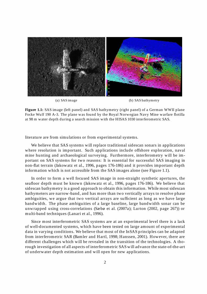
(a) SAS image (b) SAS bathymetry

Figure 1.1: SAS image (left panel) and SAS bathymetry (right panel) of a German WWII planeFocke Wulf 190 A-3. The plane was found by the Royal Norwegian Navy Mine warfare flotillaat 98 m water depth during a search mission with the HISAS 1030 interferometric SAS.

literature are from simulations or from experimental systems.

We believe that SAS systems will replace traditional sidescan sonars in applicationswhere resolution is important. Such applications include offshore exploration, navalmine hunting and archaeological surveying. Furthermore, interferometry will be im-portant on SAS systems for two reasons: It is essential for successful SAS imaging innon-flat terrain (Jakowatz et al., 1996, pages 176-186) and it provides important depthinformation which is not accessible from the SAS images alone (see Figure 1.1).

In order to form a well focused SAS image in non-straight synthetic apertures, theseafloor depth must be known (Jakowatz et al., 1996, pages 176-186). We believe thatsidescan bathymetry is a good approach to obtain this information. While most sidescanbathymeters are narrow-band, and has more than two vertically arrays to resolve phaseambiguities, we argue that two vertical arrays are sufficient as long as we have largebandwidth. The phase ambiguities of a large baseline, large bandwidth sonar can beunwrapped using cross-correlations (Sæbø et al. (2007a); Lurton (2002, page 267)) ormulti-band techniques (Lanari et al., 1996).

Since most interferometric SAS systems are at an experimental level there is a lackof well-documented systems, which have been tested on large amount of experimentaldata in varying conditions. We believe that most of the InSAS principles can be adaptedfrom interferometric SAR (Bamler and Hartl, 1998; Hanssen, 2001). However, there aredifferent challenges which will be revealed in the transition of the technologies. A tho-rough investigation of all aspects of interferometric SAS will advance the state-of-the-artof underwater depth estimation and will open for new applications.

2

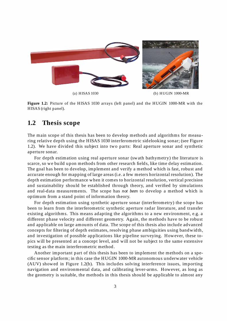
(a) HISAS 1030 (b) HUGIN 1000-MR

Figure 1.2: Picture of the HISAS 1030 arrays (left panel) and the HUGIN 1000-MR with theHISAS (right panel).

1.2 Thesis scope

The main scope of this thesis has been to develop methods and algorithms for measu-ring relative depth using the HISAS 1030 interferometric sidelooking sonar; (see Figure1.2). We have divided this subject into two parts: Real aperture sonar and syntheticaperture sonar.

For depth estimation using real aperture sonar (swath bathymetry) the literature isscarce, so we build upon methods from other research fields, like time delay estimation.The goal has been to develop, implement and verify a method which is fast, robust andaccurate enough for mapping of large areas (i.e. a few meters horizontal resolution). Thedepth estimation performance when it comes to horizontal resolution, vertical precisionand sustainability should be established through theory, and verified by simulationsand real-data measurements. The scope has not been to develop a method which isoptimum from a stand point of information theory.

For depth estimation using synthetic aperture sonar (interferometry) the scope hasbeen to learn from the interferometric synthetic aperture radar literature, and transferexisting algorithms. This means adapting the algorithms to a new environment, e.g. adifferent phase velocity and different geometry. Again, the methods have to be robustand applicable on large amounts of data. The scope of this thesis also include advancedconcepts for filtering of depth estimates, resolving phase ambiguities using bandwidth,and investigation of possible applications like pipeline surveying. However, these to-pics will be presented at a concept level, and will not be subject to the same extensivetesting as the main interferometric method.

Another important part of this thesis has been to implement the methods on a spe-cific sensor platform; in this case the HUGIN 1000-MR autonomous underwater vehicle(AUV) showed in Figure 1.2(b). This includes solving interference issues, importingnavigation and environmental data, and calibrating lever-arms. However, as long asthe geometry is suitable, the methods in this thesis should be applicable to almost any

3

interferometric sidelooking sensor on almost any platform. An important topic is a com-parison of the performance of our depth estimation algorithms with the performance ofan EM 3000 mounted on the same AUV. An EM 3000 is an advanced multibeam echosounder and represents in this case an excellent validation sensor.

In summary, this thesis advances the state-of-the-art of underwater depth estimationby describing and verifying methods for swath bathymetry and interferometry usingAUV based interferometric synthetic aperture sonar.

1.3 Thesis contribution

The contributions of this thesis to the research area of relative depth estimation usingsidelooking sonar are the following (in order of appearance):

• The design and evaluation of the HISAS sensor and the development of the FO-CUS software package for SAS processing (Hansen et al., 2010a). Much of thework during this period has contributed to the development of HISAS, whichhas become a commercially available product from Kongsberg Maritime (Fossumet al., 2008). This sensor is bundled with the FOCUS processing software, whichamong other things contains all methods described in this thesis. HISAS with FO-CUS is now sold to a number of international costumers, including two Navies.

• A thorough mathematical description of the geometry in relative seafloor depthestimation. Although equivalent methods exist, our novel description provides anapproximation-free and alternative solution. This description was first presentedin Sæbø et al. (2007b) and appears here in Section 3.1.3.

• The refined estimate of the time delay from time series with asymmetrical spectra.This method was first presented in Sæbø et al. (2007b) and appears here in Section4.1.4.

• The use of the cross-uncertainty function as a time- and dilation-estimator in swathbathymetry. This work was first presented in Sæbø et al. (2007a) and appears herein Section 4.3, 4.4 and 8.2.

• The use of a coherence weighted bilateral filter to smooth interferometric depthmaps. This method was first presented in Sæbø et al. (2009) and appears here inSection 8.4.

• The in-depth comparison of a swath bathymeter with a multibeam echo sounder,on data collected simultaneously using the same sensor platform. This study wasfirst presented in Sæbø and Langli (2010) and appears here in Section 8.5.

4

1.4 List of publications

During the writing of this thesis I have been author on three peer-review journal articles:

• T. O. Sæbø, R. E. Hansen and A. Hanssen, “Relative height estimation by cross-correlating ground-range synthetic aperture sonar images,” IEEE J. Oceanic Engi-neering, vol. 32, pp. 971-982, October 2007.

• J. Groen, R. E. Hansen, H. J. Callow, J. C. Sabel and T. O. Sæbø, “Shadow enhance-ment in synthetic aperture sonar using fixed focusing,” IEEE J. Oceanic Engineering,vol. 34, pp. 269-284, July 2009.

• T. O. Sæbø, R. E. Hansen and A. Hanssen, “Seafloor depth estimation by interfero-metric sonar using the wideband cross-uncertainty function,” to be submitted toIET Radar, sonar & navigation, 2010.

I have also been first author on ten articles published in conference proceedings:

• T. O. Sæbø and R. E. Hansen, “A comparison between interferometric SAS andinterferometric SAR,” in Proceedings of the Institute of Acoustics, Lerici, Italy, Sep-tember 2010.

• T. O. Sæbø and B. Langli, “Comparison of EM 3000 multibeam echo sounder andHISAS 1030 interferometric synthetic aperture sonar for seafloor mapping,” in Pro-ceedings of the Tenth European Conference on Underwater Acoustics, Istanbul, Turkey,pp. 451-461, July 2010.

• T. O. Sæbø, H. J. Callow and P. E. Hagen, “Pipeline inspection with synthetic aper-ture sonar,” in Proceedings of the 33th Scandinavian Symposium on Physical Acoustics,Geilo, Norway, February 2010. Online(http://www.iet.ntnu.no/en/groups/akustikk/meetings/SSPA/2010).

• T. O. Sæbø, R. E. Hansen and Ø. Midtgaard, “Filtering of high resolution interfe-rometric synthetic aperture sonar,” in Proceedings of Underwater Acoustic Measure-ments 2009, Nafplion, Greece, June 2009. CDROM (ISBN 978-960-98883-4-9).

• T. O. Sæbø, B. Langli, H. J. Callow, E. O. Hammerstad and R. E. Hansen, “Ba-thymetric capabilities of the HISAS interferometric synthetic aperture sonar,” inProceedings of OCEANS 2007 MTS/IEEE, Vancouver, Canada, October 2007.

• T. O. Sæbø, R. E. Hansen, H. J. Callow and B. Kjellesvig, “Using the cross-ambiguityfunction for improving sidelooking sonar height estimation,” in Proceedings of Un-derwater Acoustic Measurements 2007, Crete, Greece, pp. 309-316, June 2007.

• T. O. Sæbø, H. J. Callow and R. E. Hansen, “Synthetic aperture sonar interfero-metry: Experimental results from SENSOTEK,” in Proceedings of the Eight EuropeanConference on Underwater Acoustics, Carvoeiro, Portugal, pp. 829-834, June 2006.

5

• T. O. Sæbø, R. E. Hansen and H. J. Callow, “Height estimation on wideband syn-thetic aperture sonar: Experimental results from InSAS-2000,” in Proceedings ofOCEANS 2005 MTS/IEEE, Washington DC, USA, September 2005.

• T. O. Sæbø and R. E. Hansen, “Bathymetric imaging using synthetic aperturesonar,” in Proceedings of the Seventh European Conference on Underwater Acoustics,Delft, The Netherlands, pp. 1157-1162, July 2004.

• T. O. Sæbø and R. E. Hansen, “Synthetic aperture sonar interferometry,” in Procee-dings of the 27th Scandinavian Symposium on Physical Acoustics, Ustaoset, Norway,January 2004. CDROM (ISBN 82-8123-000-2).

In addition, I have contributed to 23 other conference articles related to the work pre-sented in this thesis:

• Ø. Hegrenæs, T. O. Sæbø, P. E. Hagen and B. Jalving, “Horizontal mapping accu-racy in hydrographic AUV surveys,” in Proceedings of the IEEE Autonomous Under-water Vehicles 2010, Monterey, USA, September 2010.

• H. J. Callow, R. E. Hansen, T. O. Sæbø and S. A. V. Synnes, “Autofocus for circularsynthetic aperture imaging,” in Proceedings of the Institute of Acoustics, Lerici, Italy,September 2010.

• S. A. V. Synnes, H. J. Callow, R. E. Hansen and T. O. Sæbø, “Multipass coherentprocessing on synthetic aperture sonar data,” in Proceedings of the Tenth EuropeanConference on Underwater Acoustics, Istanbul, Turkey, pp. 1307-1314, July 2010.

• R. E. Hansen, H. J. Callow, T. O. Sæbø and S. A. V. Synnes, “Challenges in sea-floor imaging and mapping with synthetic aperture sonar,” in Proceedings of theEight European conference on synthetic aperture radar, Aachen, Germany, June 2010.CDROM (ISBN 978-3-8007-3272-2).

• R. E. Hansen, T. O. Sæbø, H. J. Callow and P. E. Hagen, “Interferometric syntheticaperture sonar in pipeline inspection,” in Proceedings of OCEANS 2010 MTS/IEEE,Sydney, Australia, May 2010. CDROM (ISBN 978-1-4244-5222-4).

• Ø. Midtgaard, T. O. Sæbø and R. E. Hansen, “Estimation of target detection/ clas-sification performance using interferometric sonar coherence,” in Proceedings ofUnderwater Acoustic Measurements 2009, Nafplion, Greece, June 2009. CDROM(ISBN 978-960-98883-4-9).

• S. A. Synnes, R. E. Hansen and T. O. Sæbø, “Assessment of shallow water perfor-mance using interferometric sonar coherence,” in Proceedings of Underwater Acous-tic Measurements 2009, Nafplion, Greece, June 2009. CDROM (ISBN 978-960-98883-4-9).

6

• R. E. Hansen, H. J. Callow, T. O. Sæbø, S. A. Synnes, P. E. Hagen, T. G. Fossum andB. Langli, “Synthetic aperture sonar in challenging environments: Results from theHISAS 1030,” in Proceedings of Underwater Acoustic Measurements 2009, Nafplion,Greece, June 2009. CDROM (ISBN 978-960-98883-4-9).

• H. J. Callow, R. E. Hansen, S. A. Synnes and T. O. Sæbø, “Circular synthetic ape-rure sonar without a beacon,” in Proceedings of Underwater Acoustic Measurements2009, Nafplion, Greece, June 2009. CDROM (ISBN 978-960-98883-4-9).

• R. E. Hansen, H. J. Callow, T. O. Sæbø, P. E. Hagen and B. Langli, “High fidelitysynthetic aperture sonar products for target analysis,” in Proceedings of OCEANS2008 MTS/IEEE, Quebec, Canada, September 2008.

• T. G. Fossum, T. O. Sæbø, B. Langli, H. J. Callow, and R. E. Hansen, “HISAS 1030- high resolution interferometric synthetic aperture sonar,” in Proceedings of theCanadian Hydrographic Conference and National Surveyors Conference, Victoria, BC,Canada, May 2008.

• Ø. Midtgaard, T. O. Sæbø and H. J. Callow, “Automated recognition of short-tethered objects with interferometric synthetic aperture sonar,” in Proceedings ofOCEANS 2007 MTS/IEEE, Vancouver, Canada, October 2007.

• R. E. Hansen, H. J. Callow and T. O. Sæbø, “The effect of sound velocity variationson synthetic aperture sonar,” in Proceedings of Underwater Acoustic Measurements2007, Crete, Greece, pp. 323-330, June 2007.

• H. J. Callow, R. E. Hansen and T. O. Sæbø, “Effect of approximations in fast facto-rized backprojection in synthetic aperture imaging of spot regions,” in Proceedingsof OCEANS 2006 MTS/IEEE, Boston, MA, USA, September 2006.

• R. E. Hansen, H. J. Callow, T. O. Sæbø, P. E. Hagen and B. Langli, “Signal proces-sing for the SENSOTEK interferometric SAS: Lessons learned from HUGIN AUVtrials,” in Proceedings of the Institute of Acoustics, vol. 28, Lerici, Italy, pp. 47-56,September 2006. CDROM (ISBN 1- 901656-79-9).

• R. E. Hansen, T. O. Sæbø and H. J. Callow, “The SENSOTEK interferometric syn-thetic aperture sonar: Results from HUGIN AUV trials,” in Proceedings of the EighthEuropean Conference on Underwater Acoustics, Carvoeiro, Portugal, pp. 623-628,June 2006.

• R. E. Hansen, T. O. Sæbø, H. J. Callow and B. Langli, “Synthetic aperture so-nar imaging on HUGIN AUV: Results from SENSOTEK SAS,” in Proceedings ofthe 29th Scandinavian Symposium on Physical Acoustics, Ustaoset, Norway, January2006. CDROM (ISBN 82-8123-001-0).

7

• B. Kjellesvig, R. E. Hansen and T. O. Sæbø, “Improved height estimation for syn-thetic aperture sonar interferometry,” in Proceedings of the 29th Scandinavian Sym-posium on Physical Acoustics, Ustaoset, Norway, January 2006. CDROM (ISBN 82-8123-001-0).

• R. E. Hansen, T. O. Sæbø, H. J. Callow, P. E. Hagen and E. Hammerstad, “Syntheticaperture sonar processing for the HUGIN AUV,” in Proceedings of OCEANS 2005MTS/IEEE, Brest, France, June 2005.

• H. J. Callow, T. O. Sæbø and R. E. Hansen, “Towards robust quality assessment ofSAS imagery using the DPCA algorithm,” in Proceedings of OCEANS 2005 MTS/IEEE, Brest, France, June 2005.

• J. Groen, B. A. J. Quesson, J. C. Sabel, R. E. Hansen, H. J. Callow and T. O. Sæbø,“Simulation of high resolution mine hunting sonar measurements,” in Proceedingsof Underwater Acoustic Measurements 2005, Crete, Greece, June-July 2005.

• R. E. Hansen, T. O. Sæbø and P. E. Hagen, “Development of synthetic aperturesonar for the HUGIN AUV,” in Proceedings of the Seventh European Conference onUnderwater Acoustics, Delft, The Netherlands, pp. 1139-1144, July 2004.

• R. E. Hansen, T. O. Sæbø, K. Gade and S. Chapman, “Signal processing for AUVbased interferometric synthetic aperture sonar,” in Proceedings of OCEANS 2003MT/IEEE, San Diego, CA, USA, pp. 2438-2444, September 2003.

1.5 Outline

The outline of this thesis is as follows. Chapter 2 gives an introduction to interferometricsynthetic aperture sonar. The main topics of the chapter is imaging and interferometricprocessing, but it also covers statistics of synthetic aperture images. We conclude witha comparison of interferometric synthetic aperture radar and interferometric syntheticaperture radar (InSAR). The material presented here is a review of earlier work.

In Chapter 3 we give a thorough description of the geometry in interferometric side-looking sonar. We describe the interferometric time delay and time dilation and presenta ground-range co-registration technique which corrects for both effects. We also dis-cuss effects of aperture length and deduce the accuracy of the relative depth estimate.

In Chapter 4 we discuss time delay estimation and time dilation estimation. Weintroduce the cross-correlation function, the cross-uncertainty function and the phase-difference technique. We present a number of likely model errors, before we concludewith a short section on coherence estimation.

In Chapter 5 we describe our specific implementation of the methods presented inChapters 3 and 4. We have divided the subject into depth estimation using sidescan so-nar, depth estimation using SAS and use of relative depth estimation in SAS processing.

8

In Chapter 6 we present detailed specifications of the HISAS 1030 sonar and com-pare HISAS to a number of SAR systems. We also briefly discuss the HUGIN 1000-MRautonomous underwater vehicle.

In Chapter 7 we present a theoretical study of the horizontal resolution and verticalprecision of the relative depth estimates. We distinguished between depth estimationusing sidescan sonar and depth estimation using SAS. We verify our findings usingsimulated data.

In Chapter 8 we present results from a number of studies using experimental HISASdata. These topics are comparison of HISAS with a multibeam echo sounder, filteringof interferograms and depth maps, resolving phase ambiguities and using HISAS forpipeline inspection.

The conclusion of this thesis is presented in Chapter 9.

9

10

Chapter 2

Interferometric synthetic apertureprocessing

This chapter provides a summary of the appropriate background knowledge needed tofollow subsequent parts of this thesis. For an extensive coverage on the topic see e.g.Hanssen (2001) or Franceschetti and Lanari (1999).

2.1 Imaging

Echo imaging is an inverse problem where the goal is to construct an image which re-presents the locations of discrete targets, or the spatial distribution of a continuous para-meter related to the physical properties of a target (Soumekh, 1994, chapter 1). In sonarimaging, large-bandwidth acoustic pulses are transmitted and pulse compressed on re-ceive. The pulse compression is a matched filtering with maximizes the signal-to-noiseratio (SNR) in white Gaussian noise (DiFranco and Rubin (1980, chapter 5); Levanon(1988, chapter 5); Richards (2005, pages 161-167)). Each target in the illuminated sceneproduces an echo which after pulse compression appears as a sinc-like pattern in the re-ceived time series, dependent on the transmitted pulse form (Franceschetti and Lanari,1999, pages 15-24). We define slant-range to be the direction of the acoustic waves fora given range. Often, range and slant-range are used interchangeably. The 3 dB rangeresolution is a measure of the range-distance needed to separate two targets of equalstrength by 3 dB (Franceschetti and Lanari, 1999, page 23)

δssir =c

2B, (2.1)

where c is the speed of sound and B the signal bandwidth. To suppress sidelobes at theexpense of increased resolution we apply a mild window after the matched filter.

In this thesis we define an imaging coordinate system, where x is the coordinatealong the receiver array, r is the slant-range coordinate, z is pointing down towardsthe seafloor and y is ground-range orthogonal to x and z (the xyz system forms a right

11

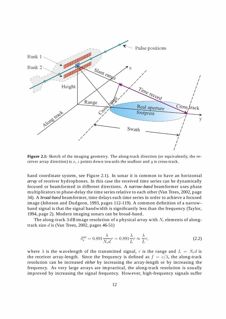
Figure 2.1: Sketch of the imaging geometry. The along-track direction (or equivalently, the re-ceiver array direction) is x, z points down towards the seafloor and y is cross-track.

hand coordinate system, see Figure 2.1). In sonar it is common to have an horizontalarray of receiver hydrophones. In this case the received time series can be dynamicallyfocused or beamformed in different directions. A narrow-band beamformer uses phasemultiplicators to phase-delay the time series relative to each other (Van Trees, 2002, page34). A broad-band beamformer, time delays each time series in order to achieve a focusedimage (Johnson and Dudgeon, 1993, pages 112-119). A common definition of a narrow-band signal is that the signal bandwidth is significantly less than the frequency (Taylor,1994, page 2). Modern imaging sonars can be broad-band.

The along-track 3 dB image resolution of a physical array with Nr elements of along-track size d is (Van Trees, 2002, pages 46-51)

δssix = 0.891λ

Nrdr = 0.891

λ

Lr ≈ λ

Lr, (2.2)

where λ is the wavelength of the transmitted signal, r is the range and L = Nrd isthe receiver array-length. Since the frequency is defined as f = c/λ, the along-trackresolution can be increased either by increasing the array-length or by increasing thefrequency. As very large arrays are impractical, the along-track resolution is usuallyimproved by increasing the signal frequency. However, high-frequency signals suffer

12

from attenuation (Brekhovskikh and Lysanov (1982, pages 9-11); Lurton (2002, pages18-26)) and will therefore decay at a shorter range.

A sidelooking imaging sonar which is based on beamforming a physical array issometimes referred to as a real aperture sonar (in contradiction to a synthetic aperturesonar). When such a sonar is moved along a path and repetitive pulses are transmitted,it is called a sidescan sonar.

2.2 Synthetic aperture processing

A real aperture sonar is limited by a range-dependent along-track resolution. In or-der to achieve high along-track resolution, one must have very high frequency andshort range. This reduces the area coverage rate and makes the sonar impractical forsurveying of large areas. A solution adapted from radar is to use synthetic apertureprocessing (Franceschetti and Lanari, 1999; Jakowatz et al., 1996). In synthetic apertureprocessing successive pings (or pulses in radar terminology) are coherently combined tosynthesize a longer array. The range-resolution is the same as for real aperture imaging

δsasir = δssir =c

2B, (2.3)

However, the along track resolution becomes

δsasix ≈ λ

2LSAr, (2.4)

where LSA is the length of the synthetic aperture, and the factor two in the denominatoris caused by the motion of the transmitter along the synthetic aperture (Lurton, 2002,page 173). The length of the synthetic aperture is limited by the beamwidth of thereceive elements

LSA ≤ λ

dr. (2.5)

This means that the maximum along-track resolution achievable is given by (Curlanderand McDonough (1991, page 16-21); Franceschetti and Lanari (1999, pages 24-31))

δsasix ≈ d

2. (2.6)

The most important property of Equation 2.6 is that it is range-independent. This isquite counter-intuitive for people trained within classical beamforming; the shorter theelement, the better the resolution. Note that the diffraction limit (Jakowatz et al., 1996,page 75) is given by λ/4, so there is no benefit in having elements smaller than λ/2.Similar to the pulse compression, we apply a mild window in the synthetic apertureprocessing to suppress along-track sidelobes in the synthetic aperture images. Figure2.2 shows an illustration of the difference between real aperture and synthetic apertureimaging.

13

Figure 2.2: Illustration of sidescan sonar imaging geometry (upper panel) and SAS imaginggeometry (lower panel).

In synthetic aperture processing one has to move less than half the receiver elementsize between pings, in order to avoid undersampling lobes (Franceschetti and Lanari,1999, pages 28-29). Since the phase velocity is a factor of 2 · 105 lower for acoustic wavesin seawater than for electromagnetic waves, this imposes an impractical limitation. Itis therefore common to use a large number of elements along-track to increase the areacoverage rate (Cutrona, 1975; Bruce, 1992).

Another serious constraint is the need for accurate navigation. Navigation errors lar-ger than a fraction of a wavelength over the synthetic aperture will cause defocus in thesynthetic aperture images (Jakowatz et al., 1996, pages 228-238). Since the length of thesynthetic aperture increases with range, the navigation constraint becomes range de-pendent. Thus the image quality is often range dependent even if the theoretical image

14

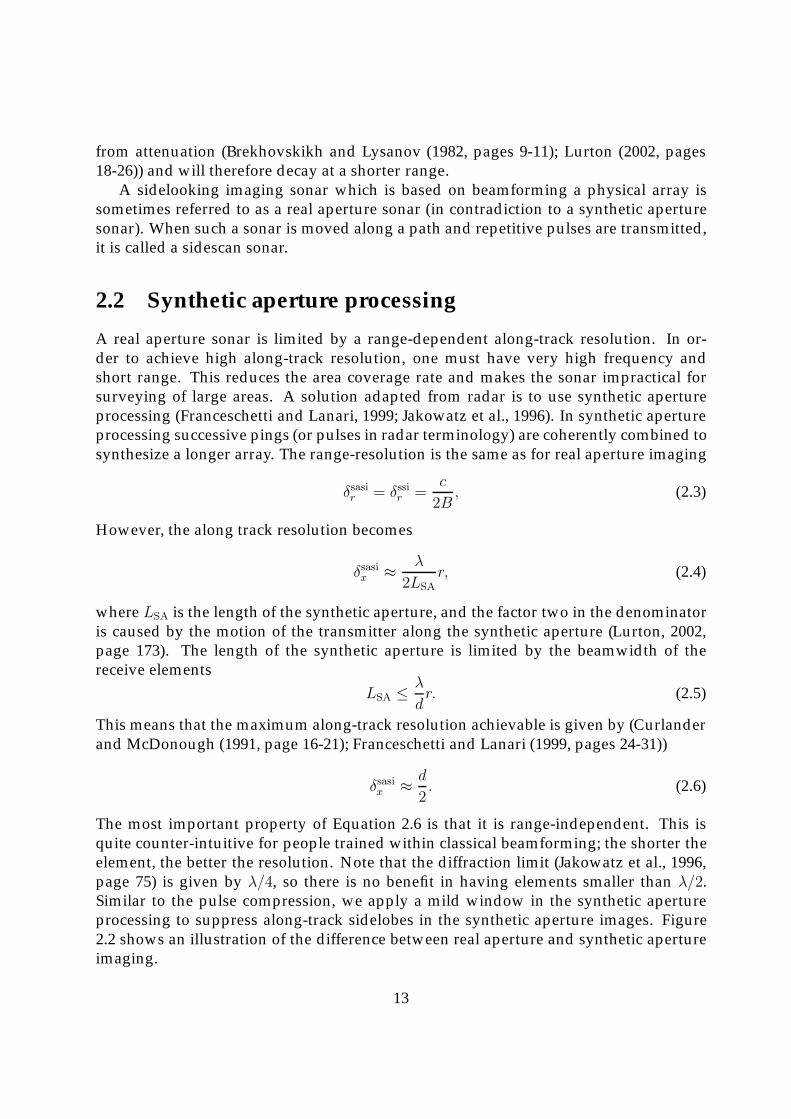
Figure 2.3: The principle of interferometry is based on estimating the time difference of arrivalof two vertically displaced receivers.

resolution is not. On small platforms such as AUVs, inertial navigation systems alonecan not provide the desired navigational accuracy, so micronavigation techniques whichuse redundancy in the data to estimate sensor translation has been developed. One ofthe most common methods is the displaced phase center antenna principle (DPCA)which uses cross-correlations on element data (Bellettini and Pinto, 2002).

Another approach adapted from SAR is autofocus, which is a method for blind cor-rection of image degradations using the complex synthetic aperture image as input.The most common technique both in SAR and SAS is called phase gradient autofocus(PGA) (Jakowatz et al. (1996, pages 251-269); Carrara et al. (1995, pages 264-268); Callow(2003)).

2.3 Interferometry

Interferometry means to determine the angular direction of an arrival signal, by meansof the time delay between the arrival of the signal at spatially separated receivers (Hans-sen, 2001; Franceschetti and Lanari, 1999). Figure 2.3 shows a simple sketch of a typicalinterferometric sonar. A single transmitter and two vertically separated receivers areused to determine the depression angle of the arriving echo.

The distance between the interferometric receivers is called the baseline. Usually, oneassumes that the baseline, D is small relative to the range so the arrival wavefronts canbe considered parallel (Hanssen, 2001, page 36). The relative depth, z is then found from

z = r(cτD

). (2.7)

where τ is the interferometric time delay between the arrival signals. The time delay isusually estimated from the phase-difference between the signals (Hanssen, 2001, page

15

15). The precision of the time delay estimate is a function of SNR, and the estimate canthus be very precise for high SNR. However, the phase-difference is ambiguous mo-dulo 2π (Ghiglia and Pritt, 1998). A number of different approaches have been madeto unwrap the phase. 2D phase unwrappers find the most likely phase assuming thatthe data are continuous (Ghiglia and Pritt, 1998), multi-receiver or multi-frequency sys-tems use redundancy to resolve the ambiguities (Hanssen, 2001, pages 72-79) and cross-correlation based methods estimates the ambiguities at the expense of poorer horizontalresolution and increased processing time (Lurton, 2002, page 267).

The accuracy of the time delay estimate is proportional to the baseline (Hanssen,2001, pages 35-38). However, increasing the baseline to much will reduce the coherencebetween the signals (Lurton, 2000) and also deteriorate the accuracy of the time delayestimate. Other limiting factors are

• Layover (Franceschetti and Lanari, 1999, page 37-41). In layover regions, thereis a mixture of signals arriving from different directions. The different directionscannot be resolved and the coherence drops.

• Shadow (Franceschetti and Lanari, 1999, page 37-41). In shadow regions, there isa lack of signal energy and a time delay can not be estimated.

• Multipath (Brekhovskikh and Lysanov, 1982, chapter 9). Signals arriving fromother directions than directly from the seafloor (e.g. via the sea surface or from anelevated object and via the seafloor) will deteriorate the time delay estimate.

In benign bathymetries, the interferometric performance is limited by baseline decorre-lation at close range and SNR at long range (Lurton, 2000). In area with large bathy-metric variations or with large man-made objects, layover, shadow and multipath willlimit the interferometric performance.

2.4 Synthetic aperture image statistics

When the image resolution is significantly larger than the wavelength of the transmittedsignal, many scatterers will contribute to the response for each resolution cell (Hanssen,2001; Oliver and Quegan, 2004, page 89-91). It is then not possible to determine theresponse of individual scatterers within a resolution cell. The result is the characteris-tic speckle response (Hanssen, 2001, page 89-91). A common method is to model themeasured reflection as a sum of many scatterers. Applying the central limit theorem,the observations can be considered complex (circular) Gaussian random variables. Thefollowing assumptions are made (Hanssen, 2001, page 89-91)

• No single scatterer should dominate the others in a resolution cell

• The phase of the individual scatterers must be uniformly distributed between −πand π. This holds since a very large phase (r � λ) is wrapped into the −π to πinterval.

16

• The phases of the individual scatterers must be uncorrelated.

• The amplitude must be independent from the phase for every scatterer. This holdsbecause the phase is a function of propagation length and is independent of thescattering mechanism

The joint probability density function (PDF) for the image amplitude, a and theimage phase, ν can be written (Hanssen, 2001, page 89-91)

p(a, ν) =

{a

2πσ2 exp(− a2

2σ2

): for a ≥ 0 and − π ≤ ν < π

0 : otherwise,(2.8)

where σ =√E{I}/2. Here I is the intensity of the resolution cell and E{I} its expecta-

tion value. The marginal PDF of a is obtained by integrating ν from −π to π.

p(a) =

{aσ2 exp

(− a2

2σ2

): for a ≥ 0

0 : otherwise.(2.9)

Equation 2.9 is the Rayleigh distribution (Hanssen, 2001, page 89-91). The marginal PDFog ν is found by integrating a from 0 to ∞

p(ν) =

{12π

: for − π ≤ ν < π0 : otherwise.

(2.10)

Equation 2.10 describes a uniform distribution. Since p(a, ν) = p(a)p(ν), a and ν areuncorrelated. The pixel intensity variation using the above model is known as speckle.The effect of speckle is often reduced by assuming ergodicity and averaging pixels inco-herently. The resulting PDF of the intensity of N averaged pixels is the χ2-distributionwith 2N degrees of freedom (Hanssen, 2001, page 89-91)

p(I;N) =I2N−1

E{I}NΓ(N)exp

(− I

E{I}), (2.11)

where Γ is the Gamma function (Rottmann, 1995). For N = 1, Equation 2.11 reduces tothe exponential PDF. For N → ∞, it equals a Gaussian PDF.

2.5 Relation to radar

The principle of synthetic aperture radar and synthetic aperture sonar is the same, butthere are fundamental differences (Hansen et al., 2010a):

• For electromagnetic signals in air, the phase velocity is typically 3 × 108 m/s. Foracoustic waves in seawater, c ≈ 1.5×103 m/s, which limits the forward velocity inSAS. In practice, it is difficult to make a stable SAS-platform with a low enough ve-locity. The solution is to use multi-element receiver arrays (Cutrona, 1975; Bruce,1992).

17

• The atmospheric attenuation of electromagnetic signals depends on the weatherconditions, but is often considered a minor effect in SAR. In SAS, however, theseawater absorbs the acoustical signal energy through viscosity and chemical pro-cesses (Brekhovskikh and Lysanov (1982, pages 9-11); Lurton (2002, pages 18-26)). This limits the range for a given frequency, as the practical range is roughlyconstant measured in wavelengths.

• The phase velocity has to be known along the wave path. In SAR the speed of lightis accurately known, but in SAS the speed of sound varies with depth (Brekhovs-kikh and Lysanov (1982, pages 2-9); Lurton (2002, pages[pages 39-41)). In coastalwaters, there are also local horizontal and temporal variations. The variation maybe as high as 2% along the wave path. The effect is two-fold: An error in the ave-rage sound speed leads to defocusing of the SAS images (Rolt and Schmidt, 1994;Hansen et al., 2007), while an error in the sound speed profile also causes positionerrors (Hegrenæs et al., 2010).

• The imaging geometry of existing SAS systems are very similar, with a swath rea-ching from nadir to roughly ten times the altitude. This geometry is very differentfrom spaceborne SAR systems, which have a much more vertical geometry. Thevertical geometry reduces the effect of shadowing, but increase the effect of fore-shortening and layover (Franceschetti and Lanari, 1999, pages 37-42). An airborneSAR system usually has an imaging geometry somewhere between a SAS and anspaceborne SAR.

• To make a diffraction limited image, the sensor position has to be known within afraction of a wavelength over the synthetic aperture. Satellite tracks are determi-nistic and accurately known within this limit, but on airborne SAR systems andSAS systems (which can not use GPS) the navigation is often a limiting factor.

While SAR, being available for decades, has reached a very high level of maturity,SAS has only recently become commercially available. This is partly due to the diffe-rences listed above. SAR interferometry is today very sophisticated, using techniquessuch as repeat-pass image collections over years and multi-baselines for tomographic(or 3D) imaging. SAS interferometry has been demonstrated successfully at numerousoccasions, but has yet to reveal its full potential. It is likely that advanced methods ininterferometric SAR will be adapted by the SAS community. Current technology trendsin SAR interferometry are:

• Differential and repeat-pass interferometry for deformation monitoring, wheremultiple images are collected over a large time span (up to years). A major li-mitation is that the effect of the atmosphere has to be estimated and compensatedfor.

• Multi-baseline SAR tomography for 3D imaging, e.g. used in forest mapping (toestimate the average height of the trees).

18

• Single pass multi-platform interferometric SAR for increased baseline and map-ping accuracy using several platforms in formation flying.

• Bistatic SAR using one moving antenna and one stationary antenna, or two mo-ving antennas.

• Multi-frequency and ultra wideband SAR for characterization of areas and targets.

• Multi-channel along-track interferometry for moving target indication.

19

20

Chapter 3

Geometry

Interferometry can be looked upon as an advanced form of stereometri (Franceschettiand Lanari, 1999, pages 167-171). Geometrical differences in signals recorded at dif-ferent positions are used to resolve the angle of arrival of the signal. In relative depthestimation using a bistatic sonar, the echo from the seafloor recorded at individual re-ceivers is exploited (Lurton, 2002, pages 266-267). This method is closely related to ra-dar interferometry (Hanssen (2001, pages 51-58); Franceschetti and Lanari (1999, pages185-195); Jakowatz et al. (1996, pages 303-317)). However, the geometry can be quitedifferent for sidelooking sonar. While a radar system may have a very large depressionangle and baseline, a sonar is usually operated close to the seafloor and with a relati-vely small interferometric baseline (see Section 6.3). Figure 3.1 shows a schematic of thegeometry for a sonar system on an autonomous underwater vehicle.

In more detail, the time delay for a location on the seafloor, τ , caused by travel pathdifferences, is converted to a direction of arrival, or a depression angle, Φ. By combi-ning this angle with the range to the seafloor we can determine the relative depth ofthe seafloor, z. A description of the relation between τ and z can be found from thevertical geometry alone, which means that a common set of equations apply for bothrelative depth estimation using sidescan sonar and interferometric SAS. However, SASinterferometry has some additional effects in the horizontal plane, due to the integra-tion along-track. We will start by describing the common vertical geometry and thendiscuss the effects of synthetic aperture processing later in this chapter.

3.1 Geometry in the vertical-plane

Figure 3.1 shows an interferometric sonar with two receivers illuminating a seafloorwith relative depth, z0. Without loss of generality, the coordinate system is chosen suchthat the transmitter is placed at origin. The upper receiver is at position (y1, z1) relativeto the transmitter and the lower receiver at (y2, z2). For a given position (y0, z0) at theseafloor, each receiver records a backscattered signal f(r(y0, z0)) where r(y0, z0) is thetwo-way range from the transmitter, to the seafloor and back to the receiver. The re-

21

y1y2 y0

z1

z2

z0

z

y

r1r0

r2

Figure 3.1: Schematic of the vertical plane of a sidelooking sonar with a transmitter at originand two receivers at positions (y1, z1) and (y2, z2). The signal is transmitted down to a position(y0, z0) at the seafloor and reflected back to the receivers. The z-axis points down toward theseafloor.

ceived signal is a geometrical transformation of a single realization of the underlyingreflectivity function of the seafloor, s(y, z).

3.1.1 Interferometric time delay

The basis of relative depth estimation and interferometry is an accurate description ofthe time delay caused by the bistatic configuration (Hanssen (2001, pages 51-58); Fran-ceschetti and Lanari (1999, pages 185-195); Jakowatz et al. (1996, pages 303-317)). FromFigure 3.1 we see that the backscattered signal for a reflector at (y, z) arrives at the tworeceivers with the time delay

τ(y, z) = t1(y, z)− t2(y, z) =1

c((r0(y, z) + r1(y, z))− (r0(y, z) + r2(y, z))),

=1

c(r1(y, z)− r2(y, z)),

(3.1)

where t1(y, z) and t2(y, z) are the receive times for receiver #1 and #2, respectively, andc is the sound velocity. The time delay, τ , is in the literature sometimes referred to as

22

the time difference of arrival (TDOA), while t1(y, z) and t2(y, z) are the time of arrivals(TOA) (Falsi et al., 2006). The ranges can be written

r0(y, z) =(y2 + z2

)1/2, (3.2a)

r1(y, z) =((y − y1)

2 + (z − z1)2)1/2, (3.2b)

r2(y, z) =((y − y2)

2 + (z − z2)2)1/2. (3.2c)

From Equations 3.1 and 3.2 it is possible to find a solution for z. Notice that only thereturn paths are different in the time delay calculation. By relocating the origin to thelower receiver and rotating the coordinate system (see Figure 3.2) the ranges can bewritten as

r1(y′, z′) =

((y′)2 + (z′ +D)

2)1/2

, (3.3a)

r2(y′, z′) =

((y′)2 + (z′)2

)1/2, (3.3b)

where D is the baseline between the receivers. The seafloor position (y′, z′), relative tothe lower receiver in the new rotated coordinate system is given by

y′ = y cosΦ0 + z sinΦ0, (3.4a)

z′ = z cosΦ0 − y sin Φ0 − D

2, (3.4b)

where Φ0 is the rotation between the (y, z)-frame and the (y′, z′)-frame, or the tilt-angleof the sonar relative to vertical. For simplicity, we have assumed that the transmitter iscentered between the receivers.

From Equations 3.1 and 3.3 we get the time delay on a functional form

τ(y′, z′) = r1(y′, z′)− r2(y

′, z′) = τ(y, z) = τ(r2) =r2c

((1 +

D(2z′ +D)

r22

)1/2

− 1

). (3.5)

The upper panel of Figure 3.3 shows the bistatic time delay as a function of range (ina non-rotated coordinate system). We see that for typical sidescan sonar of 100 kHzcenter frequency and higher (Lurton, 2002, page 264), the delay is multiple wavelengthsfor almost all ranges (a wavelength is equivalent to a delay of 0.01 ms for 100 kHz). Thismeans that the phase-differences are wrapped modulus 2π and cannot be used as anestimate for the time delay without some sort of phase unwrapping (see Section 4.6.8).An alternative is to use short-time cross-correlations along the range axis.

Inverting Equation 3.5 gives the relative seafloor depth in the rotated coordinateframe as a function of the measured time delay τ = τ(y′, z′), and the range r2 = r2(y

′, z′)

z′ = r2cτ

D

(cτ

2r2+ 1

)− D

2. (3.6)

23

y'0

D

z'0

z'

y'r1

r2

Figure 3.2: Schematic of the vertical plane of a sidelooking sonar with one receiver at origin andone receiver at a distance D above origin. The coordinate system is rotated so the two receiversboth lie along y′ = 0. The signal is reflected from a position (y ′0, z′0) at the seafloor.

Usually, the incoming sound paths can be assumed to be parallel with 2r2 � cτ , whichsimplifies the solution to

z′ ≈ r2cτ

D− D

2. (3.7)

The effect of this approximation is illustrated in the lower panel of Figure 3.3.The depth of the seafloor in a non-rotated coordinate system can now be calculated

based on simple trigonometry

z =

√r22 − (z′)2 sin Φ0 +

(z′ +

D

2

)cosΦ0 (3.8)

Another common way of solving the geometry is to use angles. For a sonar with tilt-angle Φ0, the relative depth is given by

z = r sin (Φ + Φ0), (3.9)

where the estimated depression angle relative to the tilt-angle Φ, is

Φ ≈ sin−1(cτD

). (3.10)

24

20 40 60 80 100 120 140 160 180 200

−0.05

−0.025

0

0.025

0.05

0.075

0.1

0.125

0.15

0.175

0.2

Range [m]

Del

ay b

etw

een

the

rece

iver

s [m

s]

(a) Time delay between the received signals

20 40 60 80 100 120 140 160 180 20014.95

14.96

14.97

14.98

14.99

15

Range [m]

Cal

cula

ted

seaf

loor

dep

th [m

]

Eq. 3.6Eq. 3.7

(b) Seafloor depth calculated from the time delay

Figure 3.3: Interferometric time delay and reconstructed seafloor depth. Panel (a) shows the timedelay in milliseconds between signals recorded at the interferometric receivers, as a function ofrange. Panel (b) shows the corresponding calculated seafloor depth from the time delay, as afunction of range. The solid line shows the result using Equation 3.6 and the dashed line showsthe result using Equation 3.7. In both panels we have used a sonar with c = 1500m/s, z = 15m,D = 30 cm and Φ0 = 22degrees.

25

Here we have assumed that the incoming sound ways are parallel, an approximationwhich is identical to assuming 2r2 � cτ . For Φ0 = 0, this method gives the same answeras Equation 3.7 (ignoring the D

2translation of the coordinate systems). However, it is

more difficult to find an exact answer using this approach.

3.1.2 Interferometric time dilation

In this section we study details of the interferometric time delay and show how thedelay can be interpreted as a dilation of the spatial geometry. A sidelooking sonar mea-sures a realization of the underlying seafloor reflectivity function, s(y, z), as a functionof time, t. We assume that there is only one depth for each position, i. e. s(y, z) = s(y).By replacing the bistatic sonar with a phase center antenna (PCA) (Bellettini and Pinto,2002), time is related to the one-way range through the relation t = 2r/c. Since time isonly a scaled version of range, we use the latter for convenience. We will show that thecoordinate transform from y to r can be regarded as a dilation of the spatial y-coordinate.Without loss of generality we adopt the rotated coordinate system from the previoussection and omit the apostrophe for simplicity.

A signal, g(u), is dilated relative to a reference signal, h(v) if g(u) = h(αu) for somedilation-factor α. Through the use of the chain-rule we see that the dilation-factor isgiven by

α =du

dv. (3.11)

At the receivers we measure a realization of the reflectivity function, s(y), as a functionof time or range, r(y). From Equation 3.3, we differentiate r(y) with respect to the spatialy-coordinate, which is equivalent to the Jacobian used in a one-parameter transform

dr1(y)

dy=

y

r1(y)= cosΦ1(y) = α1(y), (3.12a)

dr2(y)

dy=

y

r2(y)= cosΦ2(y) = α2(y), (3.12b)

where Φ1(y) and Φ2(y) are the depression angles for receiver #1 and #2, respectively, andα1(y) and α2(y) are the dilation-factors. The dilation-factors are functions of y, whichinduces a range-dependent dilation, equal to the usual cosine-transform between slant-range and ground-range (Jakowatz et al., 1996, pages 317-320).

We express the two time signals received at the interferometric array as

f1(r1) = s(α1(y) · r1), (3.13a)f2(r2) = s(α2(y) · r2), (3.13b)

where f1(r1) is the recorded signal at receiver #1 and f2(r2) is the recorded signal atreceiver #2. The two signals are time dilated or time scaled versions of the seafloorreflectivity function, s(y). For a constant seafloor depth, z0, and a fixed baseline, D,

26

α1 = α2 for y → ∞. From Equation 3.13 we see that there is in fact no time delaybetween the two signals, only a different dilation of the seafloor reflectivity function.However, when comparing a small subset of two signals dilated differently from anorigin outside the selected subset, one can perceive the dilation as a delay and a localdilation. The upper panel of Figure 3.4 shows the dilation of the seafloor reflectivityfunction for the two receivers. The dilation is almost identical for the two receiverssince z > D.

In seafloor depth estimation, the relative dilation between f1(r) and f2(r) is moreimportant than the dilation of the seafloor reflectivity function, s(y), itself. By using thesignal at receiver #2 as a reference signal and differentiating r1(y) with respect to r2(y)we get

α(y) =dr1(y)

dr2(y)=

(dr1(y)

dy

)(dr2(y)

dy

)=

(y2 + z2

y2 + (z +D)2

)1/2

, (3.14)

where α(y) is the relative time dilation between the received signals. Equation 3.14shows that the dilation-factor is unity for D = 0 or for y → ∞, which is consistentwith our intuition. The lower panel of Figure 3.4 shows the relative dilation betweenthe signals in a non-rotated coordinate frame. Notice the rapid decrease in the dilation-factor for close ranges.

To be able to resolve the seafloor depth at different positions, we divide the receivedtime series into a number of time intervals. The relative dilation around a position y0becomes

α(y0 ±Δy) =

((y0 ±Δy)2 + z2

(y0 ±Δy)2 + (z +D)2

)1/2

≈(

y20 + z2

y20 + (z +D)2

)1/2

= α(y0), (3.15)

where the assumption (y20 + z2

)� Δy(2y0 +Δy) (3.16)

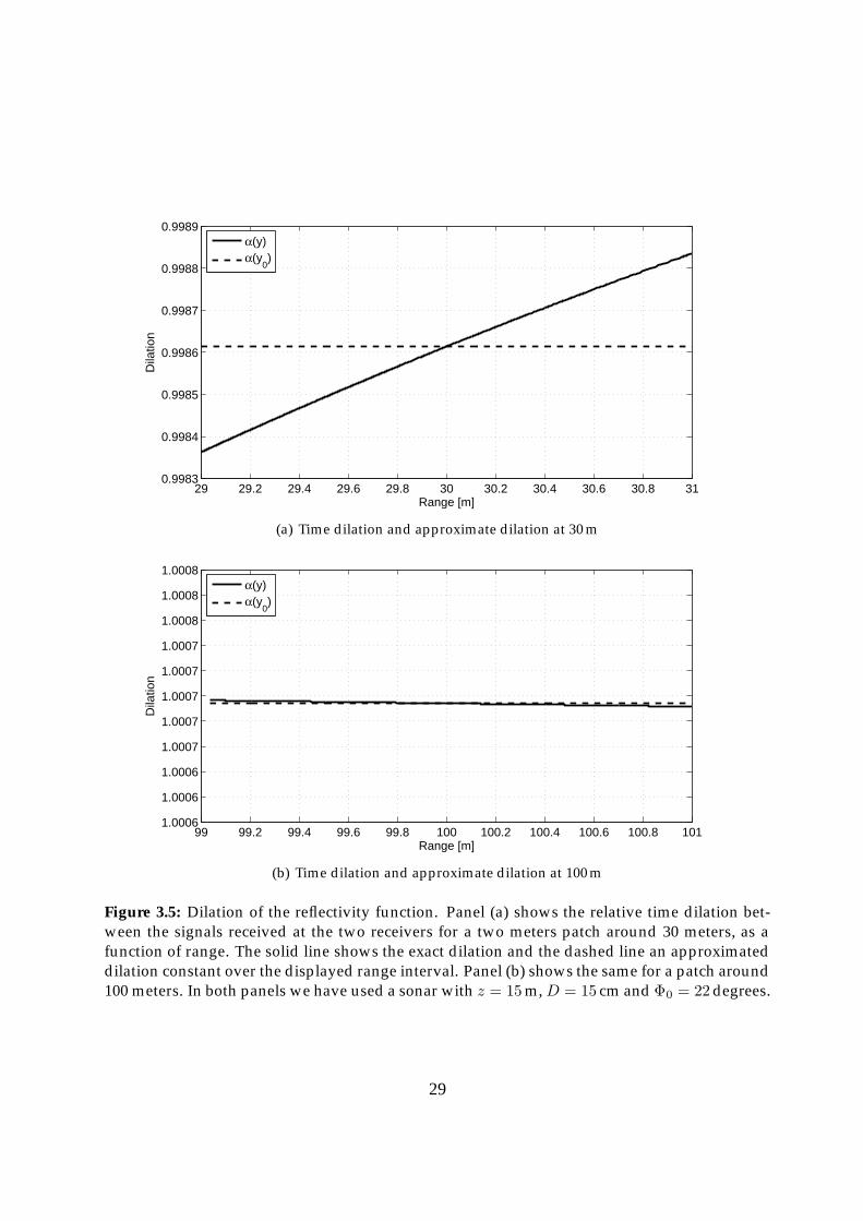
gives the approximate form. This assumption is approximately equivalent to r2 � 2Δy.Hence, the time dilation can only be regarded as constant for ranges that are large com-pared to the patch length. Figure 3.5 shows the comparison between the approximateddilation and the exact dilation for patches at 30 and 100 meters. The patch length istwo meters in both cases. While the approximation is very good at 100 meters, it issignificantly less accurate at 30 meters.

We have now established the following properties for our interferometric model:

• The received signals are time dilated versions of the seafloor reflectivity functionwith α1(y) and α2(y) as dilation-factors for receiver #1 and #2, respectively (seeEquation 3.12).

• There is a relative dilation given by α(y) between the signals received at receiver#1 and receiver #2 (see Equation 3.14).

27

20 40 60 80 100 120 140 160 180 2000.4

0.5

0.6

0.7

0.8

0.9

1

1.1

Range [m]

Dila

tion

betw

een

the

seaf

loor

and

the

rece

ived

sig

nals

Receiver 1Receiver 2

(a) Time dilation between the seafloor and the received signals

20 40 60 80 100 120 140 160 180 2000.982

0.984

0.986

0.988

0.99

0.992

0.994

0.996

0.998

1

1.002

Range [m]

Dila

tion

betw

een

the

two

rece

ived

sig

nals

(b) Relative dilation between the two received signals

Figure 3.4: Dilation of the reflectivity function. Panel (a) shows the time dilation of the seafloorreflectivity function seen by the two receivers as a function of range. Circles show the dilationseen by receiver #1 and squares the dilation seen by receiver #2. Panel (b) shows the relativedilation between the two signals as a function of range. In both panels we have used a sonarwith c = 1500m/s, z = 15m, D = 30 cm and Φ0 = 22degrees.

28

29 29.2 29.4 29.6 29.8 30 30.2 30.4 30.6 30.8 310.9983

0.9984

0.9985

0.9986

0.9987

0.9988

0.9989

Range [m]

Dila

tion

α(y)α(y

0)

(a) Time dilation and approximate dilation at 30 m

99 99.2 99.4 99.6 99.8 100 100.2 100.4 100.6 100.8 1011.0006

1.0006

1.0006

1.0007

1.0007

1.0007

1.0007

1.0007

1.0008

1.0008

1.0008

Range [m]

Dila

tion

α(y)α(y

0)

(b) Time dilation and approximate dilation at 100 m

Figure 3.5: Dilation of the reflectivity function. Panel (a) shows the relative time dilation bet-ween the signals received at the two receivers for a two meters patch around 30 meters, as afunction of range. The solid line shows the exact dilation and the dashed line an approximateddilation constant over the displayed range interval. Panel (b) shows the same for a patch around100 meters. In both panels we have used a sonar with z = 15m, D = 15 cm and Φ0 = 22degrees.

29

• The relative dilation can be approximated as constant over a small patch, i.e.,α(y ±Δy) ≈ α(y) (see Equation 3.15).

• In effect, the relative dilation causes a time delay, τ(y), between the two receiversfor an echo from the same seafloor location (see Equation 3.5).

3.1.3 Depth estimation in co-registrated ground-range

As we saw in the previous section, interferometric signals are both time shifted (Lur-ton, 2000) and time dilated (Gatelli et al., 1994) relative to each other. In Section 4.2we present an estimator suited for time delay estimation on such signals. A differentapproach is to use a priori information to eliminate most of the shift and dilation. Thismethod is in many cases desirable because

• Pre-processing the data increases the coherence between the signals

• Standard time delay estimators (like cross-correlation or phase-differencing) canbe used directly

• High quality a priori data are available from the previous estimate since the sea-floor are varying slowly relative to the platform motion

• Fast 1D-interpolation along the range axis is usually sufficient

An effect we have to take into account when compensating for the dilation is a changeof the effective frequency of the signals. We consider this effect in detail in Section 5.1.1.

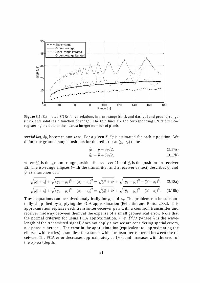
In Figure 3.6 we demonstrate the potential improvement in SNR by beamformingonto an a priori bathymetry. The maximum cross-correlation coefficients in the time de-lay estimation is converted to SNR according to Equation 4.17. The results are from aMonte Carlo simulation of 5000 realizations, with the correlation performed both di-rectly in slant-range and after beamforming onto an estimated seafloor depth (with fivemeters induced depth-error). Use of this (poor) a priori information provides a signi-ficant improvement in SNR, as can be seen in Figure 3.6. Another improvement isachieved by using the first estimate to correct for footprint shift, and thereafter cor-relate again (a simple beamforming). The correction co-registers the data to the nearestinteger number of pixels, and provides a significant SNR improvement. Note that theoscillations in the iterated correlations are caused by the discrete grid applied in the co-registration, and may be reduced by increasing the sampling frequency or by using animproved sub-pixel co-registration technique (the SNR will then approach the peaks ofthe oscillations).

Figure 3.7 illustrates how the data is re-gridded down onto an a priori seafloor depth,z. This method is a simple co-registration (Jakowatz et al., 1996, pages 288-302) wherefeatures are shifted onto the same positions in the two data-sets. If the seafloor is correct(i.e. z = z0 in Figure 3.7), y = y0 and δy = 0. When z �= z0, y differs from y0 and the

30

20 40 60 80 100 120 140 160 1805

15

25

35

45

55

Range [m]

SN

R [d

B]

Slant−rangeGround−rangeSlant−range iteratedGround−range iterated

Figure 3.6: Estimated SNRs for correlations in slant-range (thick and dashed) and ground-range(thick and solid) as a function of range. The thin lines are the corresponding SNRs after co-registering the data to the nearest integer number of pixels.

spatial lag, δy, becomes non-zero. For a given z, δy is estimated for each y-position. Wedefine the ground-range positions for the reflector at (y0, z0) to be

y1 = y − δy/2, (3.17a)y2 = y + δy/2, (3.17b)

where y1 is the ground-range position for receiver #1 and y2 is the position for receiver#2. The iso-range ellipses (with the transmitter and a receiver as foci) describes y1 andy2 as a function of z√

y20 + z20 +

√(y0 − y1)

2 + (z0 − z1)2 =√y21 + z2 +

√(y1 − y1)

2 + (z − z1)2, (3.18a)√

y20 + z20 +

√(y0 − y2)

2 + (z0 − z2)2 =√y22 + z2 +

√(y2 − y2)

2 + (z − z2)2. (3.18b)

These equations can be solved analytically for y0 and z0. The problem can be substan-tially simplified by applying the PCA approximation (Bellettini and Pinto, 2002). Thisapproximation replaces each transmitter-receiver pair with a common transmitter andreceiver midway between them, at the expense of a small geometrical error. Note thatthe normal criterion for using PCA approximation, r D2/λ (where λ is the wave-length of the transmitted signal) does not apply since we are considering spatial errors,not phase coherence. The error in the approximation (equivalent to approximating theellipses with circles) is smallest for a sonar with a transmitter centered between the re-ceivers. The PCA error decreases approximately as 1/r2, and increases with the error ofthe a priori depth.

31

y1y2 y0

z1

z2

z0

z

y

r1r0

r2

zδy

y

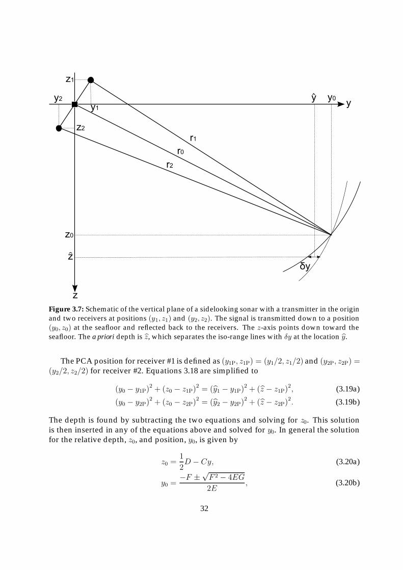
Figure 3.7: Schematic of the vertical plane of a sidelooking sonar with a transmitter in the originand two receivers at positions (y1, z1) and (y2, z2). The signal is transmitted down to a position(y0, z0) at the seafloor and reflected back to the receivers. The z-axis points down toward theseafloor. The a priori depth is z, which separates the iso-range lines with δy at the location y.

The PCA position for receiver #1 is defined as (y1P, z1P) = (y1/2, z1/2) and (y2P, z2P) =(y2/2, z2/2) for receiver #2. Equations 3.18 are simplified to

(y0 − y1P)2 + (z0 − z1P)

2 = (y1 − y1P)2 + (z − z1P)

2, (3.19a)

(y0 − y2P)2 + (z0 − z2P)

2 = (y2 − y2P)2 + (z − z2P)

2. (3.19b)

The depth is found by subtracting the two equations and solving for z0. This solutionis then inserted in any of the equations above and solved for y0. In general the solutionfor the relative depth, z0, and position, y0, is given by

z0 =1

2D − Cy, (3.20a)

y0 =−F ±√

F 2 − 4EG

2E, (3.20b)

32

0 5 10 15 20 25 30 35 40 45 50−0.2

−0.1

0

0.1

0.2

0.3

0.4

0.5

0.6

0.7

0.8

z [m]

z est−

z [m

m]

z=15mz=50mz=150m

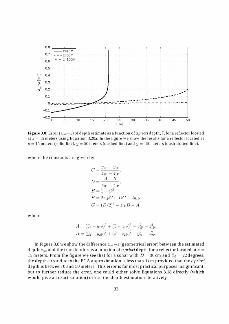
Figure 3.8: Error (zest−z) of depth estimate as a function of a priori depth, z, for a reflector locatedat z = 15 meters using Equation 3.20a. In the figure we show the results for a reflector located aty = 15 meters (solid line), y = 50 meters (dashed line) and y = 150 meters (dash-dotted line).

where the constants are given by

C =y2P − y1Pz2P − z1P

,

D =A− B

z2P − z1P,

E = 1 + C2,

F = 2z1PC −DC − 2y1P,

G = (D/2)2 − z1PD − A,

where

A = (y1 − y1P)2 + (z − z1P)

2 − y21P − z21P,

B = (y2 − y2P)2 + (z − z2P)

2 − y22P − z22P.

In Figure 3.8 we show the difference zest−z (geometrical error) between the estimateddepth zest and the true depth z as a function of a priori depth for a reflector located at z =15 meters. From the figure we see that for a sonar with D = 30 cm and Φ0 = 22degrees,the depth-error due to the PCA approximation is less than 1 cm provided that the a prioridepth is between 0 and 50 meters. This error is for most practical purposes insignificant,but to further reduce the error, one could either solve Equations 3.18 directly (whichwould give an exact solution) or run the depth estimation iteratively.

33

z0

z

y

r1

r2(1)

(2)

Figure 3.9: Illustration of a simple two-step co-registration technique. The data from one ofthe receivers are interpolated onto an a priori seafloor (1) and then interpolated back onto thegeometry of the other receiver (2).

3.1.4 Co-registration in slant-range

An alternative co-registration method, extensively used in SAR, is to use image featuresto eliminate the relative shift and dilation (Fornaro and Franceschetti, 1995). Instead ofusing an a priori depth, common features are identified in the two images and one ofthe images (the slave) is interpolated to match the other (the master). Usually, a warpingfunction describing shift, dilation and rotation is calculated from a set of control pointsor distinctive image features (Hong et al. (2006); Jakowatz et al. (1996, Pages 293-298)).Since the images are in slant-range, the phase-differences are directly proportional tothe time delay in Equation 3.5, and Equation 3.6 can be used to estimate the relativeseafloor depth. The advantage with this method is that a priori depth information isunnecessary. The drawback is that the warping function can be difficult to obtain if theSNR in the images is marginal.

By combining the a priori co-registration technique from Section 3.1.3 with slant-range geometry, it is easy to implement a slant-range co-registration technique basedon a priori depth information. One intuitive approach is to interpolate the data from oneof the receivers onto an a priori seafloor (step 1 in Figure 3.9) and then reverse interpolatethe results back to the other receiver (step 2 in Figure 3.9)

34

slavesrsr to gr−−−−−−−−→

slave geometryslavegr

gr to sr−−−−−−−−−→master geometry

slaveco−registeredsr , (3.21)

where sr means slant-range and gr ground-range. The geometrical conversions can bedescribed by Equations 3.2. To reduce errors the two interpolations can be merged.However, we have chosen ground-range as our preferred coordinate system for depthestimation and will not pursue this subject further.

3.2 Geometry in the horizontal plane

So far we have discussed the geometry in the range-depth plane. The description isonly dependent on the spatial locations of the receivers relative to the transmitter, andthe relative depth of the seafloor. In the along-track horizontal plane, depth estimationmay also be effected by aperture length.

A beamforming algorithm delays or migrates the received data onto an grid, whichflattens the polar properties of the data. In the case of a full length synthetic aperture, theiso-phase curves are independent of along-track position, i.e. the vertical cross-sectionwe considered in Section 3.1 is valid along the y-axis, independent of x. We identifythree cases: An infinitesimal aperture (an omni-directional hydrophone), a small aper-ture (a physical aperture) and an infinite aperture (a synthetic aperture). Figure 3.10illustrates the iso-phase curves for these three cases. An infinitesimal receiver has cy-lindrical symmetry with large x-dependence. An infinite aperture, on the other hand,has plane iso-phase curves (pick any point on the aperture and it looks the same). Thismeans that somewhere between these extremities there is a transition. Figure 3.10 showsthat for a slice along line A (x = 0) all the sonars behave identically, but for a slice alongline B (x �= 0) the phases are scaled relative to the broadside direction. This scaling mayaffect the time delay estimate of a bathymetric multibeam sidescan sonar with parallellines.

A non-rigorous consideration of the importance of the scaling factor can be foundfrom simple geometry. We start by assuming circular geometry and define a scalingfactor G = yof/ybs, where ybs is the y-coordinate of the iso-phase line at broadside andyof is the y-coordinate of the same iso-phase line offset xof from broadside. In Figure3.10 this corresponds to where the lines A and B cross one of the iso-phase lines. Fromthe left panel of Figure 3.11 we see that

yof =(y2bs − x2of

)−1/2, (3.22a)

G =

(y2bs − x2ofy2bs

)−1/2

, (3.22b)

where G is bounded between zero and one, and is equal to one for xof = 0. Clearly, thescaling is important for this geometry. For example, xof/ybs = 0.1 gives a five percentscaling of the time delay estimate, which easily translates to tens of cm in depth-error.

35

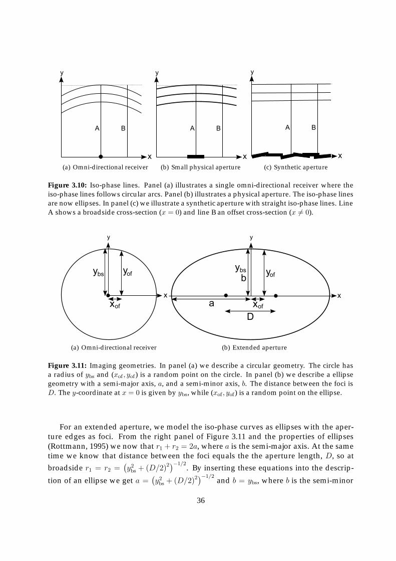
(a) Omni-directional receiver (b) Small physical aperture (c) Synthetic aperture

Figure 3.10: Iso-phase lines. Panel (a) illustrates a single omni-directional receiver where theiso-phase lines follows circular arcs. Panel (b) illustrates a physical aperture. The iso-phase linesare now ellipses. In panel (c) we illustrate a synthetic aperture with straight iso-phase lines. LineA shows a broadside cross-section (x = 0) and line B an offset cross-section (x �= 0).

x

y

xof

ybs yof

(a) Omni-directional receiver

x

y

xof

ybs yof

a

b

D

(b) Extended aperture

Figure 3.11: Imaging geometries. In panel (a) we describe a circular geometry. The circle hasa radius of ybs and (xof , yof ) is a random point on the circle. In panel (b) we describe a ellipsegeometry with a semi-major axis, a, and a semi-minor axis, b. The distance between the foci isD. The y-coordinate at x = 0 is given by ybs, while (xof , yof ) is a random point on the ellipse.

For an extended aperture, we model the iso-phase curves as ellipses with the aper-ture edges as foci. From the right panel of Figure 3.11 and the properties of ellipses(Rottmann, 1995) we now that r1 + r2 = 2a, where a is the semi-major axis. At the sametime we know that distance between the foci equals the the aperture length, D, so at

broadside r1 = r2 =(y2bs + (D/2)2

)−1/2. By inserting these equations into the descrip-

tion of an ellipse we get a =(y2bs + (D/2)2

)−1/2and b = ybs, where b is the semi-minor

36

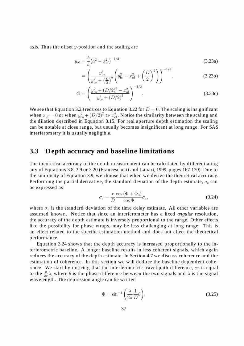
axis. Thus the offset y-position and the scaling are

yof =b

a

(a2 − x2of

)−1/2 (3.23a)

=

(y2bs

y2bs +(D2

)2(y2bs − x2of +

(D

2

)2))−1/2

, (3.23b)

G =

(y2bs + (D/2)2 − x2ofy2bs + (D/2)2

)−1/2

. (3.23c)

We see that Equation 3.23 reduces to Equation 3.22 forD = 0. The scaling is insignificantwhen xof = 0 or when y2bs + (D/2)2 � x2of . Notice the similarity between the scaling andthe dilation described in Equation 3.15. For real aperture depth estimation the scalingcan be notable at close range, but usually becomes insignificant at long range. For SASinterferometry it is usually negligible.

3.3 Depth accuracy and baseline limitations

The theoretical accuracy of the depth measurement can be calculated by differentiatingany of Equations 3.8, 3.9 or 3.20 (Franceschetti and Lanari, 1999, pages 167-170). Due tothe simplicity of Equation 3.9, we choose that when we derive the theoretical accuracy.Performing the partial derivative, the standard deviation of the depth estimate, σz canbe expressed as

σz =r

D

cos (Φ + Φ0)

cosΦστ , (3.24)

where στ is the standard deviation of the time delay estimate. All other variables areassumed known. Notice that since an interferometer has a fixed angular resolution,the accuracy of the depth estimate is inversely proportional to the range. Other effectslike the possibility for phase wraps, may be less challenging at long range. This isan effect related to the specific estimation method and does not effect the theoreticalperformance.

Equation 3.24 shows that the depth accuracy is increased proportionally to the in-terferometric baseline. A longer baseline results in less coherent signals, which againreduces the accuracy of the depth estimate. In Section 4.7 we discuss coherence and theestimation of coherence. In this section we will deduce the baseline dependent cohe-rence. We start by noticing that the interferometric travel-path difference, cτ is equalto the θ

2πλ, where θ is the phase-difference between the two signals and λ is the signal

wavelength. The depression angle can be written

Φ = sin−1

(λ

2π

1

Dθ

). (3.25)

37

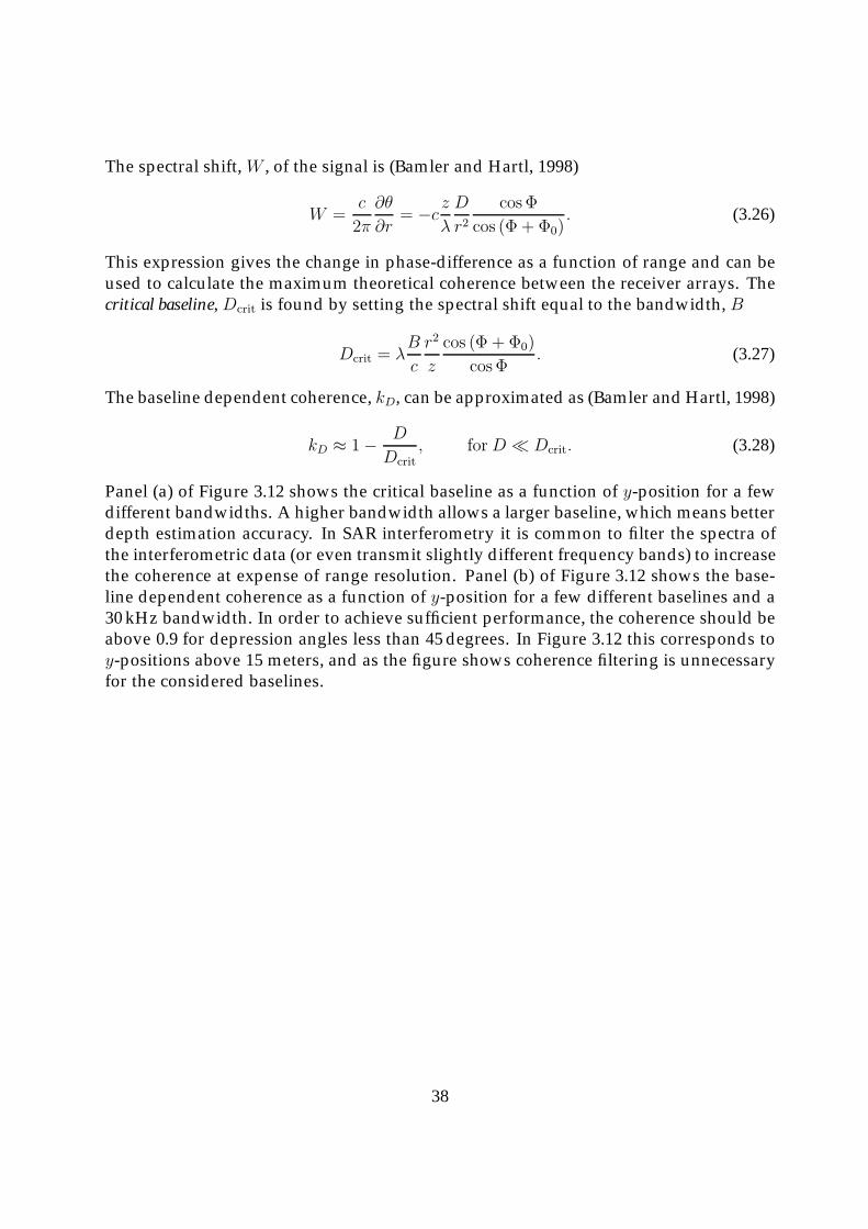
The spectral shift, W , of the signal is (Bamler and Hartl, 1998)

W =c

2π

∂θ

∂r= −c z

λ

D

r2cosΦ

cos (Φ + Φ0). (3.26)

This expression gives the change in phase-difference as a function of range and can beused to calculate the maximum theoretical coherence between the receiver arrays. Thecritical baseline, Dcrit is found by setting the spectral shift equal to the bandwidth, B

Dcrit = λB

c

r2

z

cos (Φ + Φ0)

cosΦ. (3.27)

The baseline dependent coherence, kD, can be approximated as (Bamler and Hartl, 1998)

kD ≈ 1− D

Dcrit, forD Dcrit. (3.28)

Panel (a) of Figure 3.12 shows the critical baseline as a function of y-position for a fewdifferent bandwidths. A higher bandwidth allows a larger baseline, which means betterdepth estimation accuracy. In SAR interferometry it is common to filter the spectra ofthe interferometric data (or even transmit slightly different frequency bands) to increasethe coherence at expense of range resolution. Panel (b) of Figure 3.12 shows the base-line dependent coherence as a function of y-position for a few different baselines and a30 kHz bandwidth. In order to achieve sufficient performance, the coherence should beabove 0.9 for depression angles less than 45 degrees. In Figure 3.12 this corresponds toy-positions above 15 meters, and as the figure shows coherence filtering is unnecessaryfor the considered baselines.

38

0 20 40 60 80 100 120 140 160 180 20010

0

101

102

103

104

Y position [m]

Crit

ical

bas

elin

e [m

]

B=15 kHzB=30 kHzB=60 kHz

(a) Critical baseline

0 20 40 60 80 100 120 140 160 180 2000.8

0.82

0.84

0.86

0.88

0.9

0.92

0.94

0.96

0.98

1

Y position [m]

Bas

elin

e de

pend

ent c

oher

ence

D=15 cmD=30 cmD=60 cm

(b) Coherence

Figure 3.12: Baseline limitations. Panel (a) shows the critical baseline as a function of y-positionfor bandwidths of 15 kHz (solid), 30 kHz (dashed) and 60 kHz (dotted). The sonar is at an al-titude of 15 meters with λ = 0.015 cm and Φ0 = 22degrees. Panel (b) shows the baseline de-pendent coherence as a function of y-position for baselines of 15 cm (solid), 30 cm (dashed) and60 cm (dotted) for a 30 kHz sonar.

39

40

Chapter 4

Time delay estimation

In the previous chapter we showed that the time delay between the two interferome-tric signals is required in order to estimate the relative seafloor depth. In single-passinterferometry (Jakowatz et al. (1996, pages 280-282); Franceschetti and Lanari (1999,pages 31-37)), the accuracy of the estimated bathymetry is almost always limited by theaccuracy of the time delay estimate. In repeat-pass interferometry (Hanssen, 2001, page2) additional factors like co-registration and environmental corrections can be more im-portant (Franceschetti and Lanari, 1999, Pages 173-178).

In synthetic aperture processing, time delay estimation occurs at numerous locations(Shippey et al., 1998). Micronavigation techniques use some form of time delay estima-tion. DPCA (Bellettini and Pinto, 2002) is based on time delay estimation on 1D timeseries of complex data, and very similar to the methods described in the first part ofthis chapter. Map-drift (Carrara et al., 1995, Pages 246-260) is based on image correla-tion methods, either on complex or magnitude data. Although the displacement of theimages can be ascribable to several effects, the algorithms are often similar to interfe-rometry (the difference is often that in map-drift you estimate a single offset betweenthe images, valid for the whole image, while in interferometry you estimate a delay foreach pixel). After the data are beamformed, techniques like shear averaging (Fienup,1989) and PGA (Jakowatz et al. (1996, page 251); Callow (2003)) use phase-differencesto autofocus the image. As we will show in this chapter, phase-differencing is a simpleand efficient estimation method for interferometric systems.

In this chapter we discuss three different time delay estimators: the cross-correlationfunction (CCF), the cross-uncertainty function (CUF) and phase-differencing. We showthat the cross-correlation function is a special case of the cross-uncertainty function andthat phase-differencing is a special case of the cross-correlation function. We present si-mulation results showing situations where one has to use cross-uncertainty functionin order to avoid strong decorrelation. However, by co-registrating the data in ad-vance (see Section 3.1.3) the cross-uncertainty function can be replaced by the (muchfaster) cross-correlation function without loss of accuracy. If the co-registration is accu-rate within a fraction of a resolution cell, a full correlation is unnecessary and phase-differencing will provide a fast solution.

41

4.1 Cross-correlation of signals with relative delay

Assume for now that the time dilation between the interferometric signals is negligibleand can be interpreted as a time delay for small subsets of the data. The received signalscan then be expressed as a function of time (or equivalently, a function of range)

f1(t) = s(t) + n1(t), (4.1a)f2(t) = s(t− δt) + n2(t), (4.1b)

where we have ignored the time dilation and advanced f2(t) instead of delaying f1(t).The random processes n1(t) and n2(t) model the random noise recorded by the receivers.The statistical cross-correlation function of two random signals f1(t) and f2(t) is givenby (Peebles (2001, pages 188-190); Shiavi (1999, page 355))

Rf1f2(t, t− τ) = E{f1(t)f ∗2 (t− τ)}, (4.2)

where E{·} denotes the statistical expectation or ensemble average operator. We furtherassume that the signals are jointly wide-sense stationary such that the cross-correlationfunction is a function of time difference, or local time τ , but not of absolute or globaltime t

Rf1f2(t, t− τ) = Rf1f2(τ). (4.3)

By assuming that the noise processes n1(t) and n2(t) are jointly uncorrelated zero-mean processes, and that both noise processes are uncorrelated with the signal s(t), wefind that the cross-correlation function simplifies to

Rf1f2(τ) = E{s1(t)s∗2(t− δt− τ)}. (4.4)

If we now invoke the ergodic hypothesis, we may replace expectation operators withtime averages, which yields the following useful formulation for the cross-correlationfunction

Rf1f2(τ) = limT→∞

1

2T

∫ T

−T

s(t)s∗(t− δt− τ) dt

= Rss(δt + τ).

(4.5)

The auto-correlation function Rss(τ) has its maximum at the origin, which meansthat the cross-correlation between f1(t) and f2(t) has its maximum for τ = −δt, i.e.,

Rf1f2(τ = −δt) = Rss(0). (4.6)

The delay between the signals in additive zero-mean noise can therefore be found bylocating the peak in the cross-correlation function between the two signals.

The echoes from the seafloor received by the two receivers in the interferometricsonar are not jointly wide-sense stationary. It is the non-stationarity we exploit when we

42

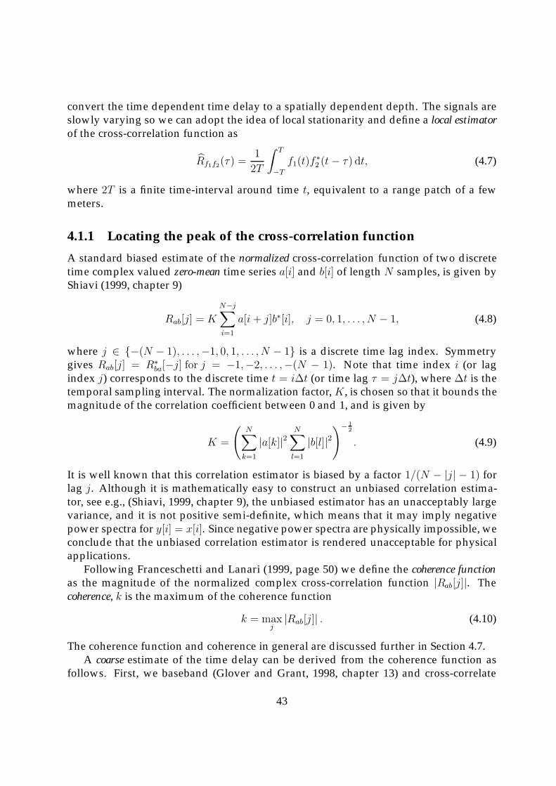
convert the time dependent time delay to a spatially dependent depth. The signals areslowly varying so we can adopt the idea of local stationarity and define a local estimatorof the cross-correlation function as

Rf1f2(τ) =1

2T

∫ T

−T

f1(t)f∗2 (t− τ) dt, (4.7)

where 2T is a finite time-interval around time t, equivalent to a range patch of a fewmeters.

4.1.1 Locating the peak of the cross-correlation function

A standard biased estimate of the normalized cross-correlation function of two discretetime complex valued zero-mean time series a[i] and b[i] of length N samples, is given byShiavi (1999, chapter 9)

Rab[j] = K

N−j∑i=1

a[i+ j]b∗[i], j = 0, 1, . . . , N − 1, (4.8)

where j ∈ {−(N − 1), . . . ,−1, 0, 1, . . . , N − 1} is a discrete time lag index. Symmetrygives Rab[j] = R∗

ba[−j] for j = −1,−2, . . . ,−(N − 1). Note that time index i (or lagindex j) corresponds to the discrete time t = iΔt (or time lag τ = jΔt), where Δt is thetemporal sampling interval. The normalization factor, K, is chosen so that it bounds themagnitude of the correlation coefficient between 0 and 1, and is given by

K =

(N∑k=1

|a[k]|2N∑l=1

|b[l]|2)− 1

2

. (4.9)

It is well known that this correlation estimator is biased by a factor 1/(N − |j| − 1) forlag j. Although it is mathematically easy to construct an unbiased correlation estima-tor, see e.g., (Shiavi, 1999, chapter 9), the unbiased estimator has an unacceptably largevariance, and it is not positive semi-definite, which means that it may imply negativepower spectra for y[i] = x[i]. Since negative power spectra are physically impossible, weconclude that the unbiased correlation estimator is rendered unacceptable for physicalapplications.

Following Franceschetti and Lanari (1999, page 50) we define the coherence functionas the magnitude of the normalized complex cross-correlation function |Rab[j]|. Thecoherence, k is the maximum of the coherence function

k = maxj

|Rab[j]| . (4.10)

The coherence function and coherence in general are discussed further in Section 4.7.A coarse estimate of the time delay can be derived from the coherence function as

follows. First, we baseband (Glover and Grant, 1998, chapter 13) and cross-correlate

43

complex subset of the recorded data. Thereafter, a simple search gives a coarse timedelay estimate τc through

τc = jcΔt, where jc = argmaxj

{|Rab[j]|}. (4.11)

Hence, the coarse time delay estimate corresponds to the peak of the discrete time co-herence function. Notice that k = |Rab[jc]|. The estimate can be improved by increasingthe sampling frequency of the data collection system, or by interpolation of the cohe-rence function (or its logarithm) by means of a parabolic fit (Moddemeijer, 1991; Holm,1993). Alternatively, the phase in the cross-correlation function can be used to improvethe time delay estimate.

Since a correlation function at carrier frequency has the property that the phaseis zero at the true coherence peak, we exploit this by mixing the phase of the cross-correlation at the location of the coherence peak up to carrier frequency again (i.e.,we undo the basebanding by multiplying with a complex exponential). The measu-red phase at the coarse time lag estimate will in general deviate from zero. Hence, thismeasured phase deviation can be used to deduce the time delay deviation of the coarsetime delay by

Δτ = −arg{Rab[jc]e

j2πf0τc}

2πf0, (4.12)

where f0 is the center frequency of the signal. We now correct the coarse time delayestimate by this delay deviation, and based on this discussion, propose the followingestimator for the fine time lag

τf = τc +Δτ. (4.13)

The probability of 2π wrap errors in the fine estimate is minimized, but may still oc-cur since the 3 dB resolution of the coherence peak is 1/B while the wrap interval is1/f0. B is here the bandwidth of the signal. For systems with B < f0, super-resolutionis in principle required to avoid wrap-errors. This can be achieved by upsampling thecross-correlation function (Mitra, 2002, pages 47-48), provided the SNR is sufficientlylarge. Even though the coarse estimate may be too inaccurate to determine the correct2π-interval, the phase can still be reliable. A 2π-correction to the phase can thereforebe applied, provided one has a priori knowledge to substantiate this. It should be noti-ced that the same performance can be achieved by cross-correlating the real signals atcarrier frequency, but then the 2π problem is replaced by the problem of selecting thecorrect coherence peak (since the correlation function of two real signals looks like ahigh-frequency modulation of the magnitude of the corresponding complex correlationfunction).

To avoid interpolation errors, upsampling should always be performed on baseban-ded data rather than on data at carrier frequency (Hawkins, 1996, chapter 4). Thereforeone should always correlate basebanded time series and correct the phase of the coarsecorrelation peak only, as showed in Equation 4.12, rather than correlating the time seriesat carrier frequency and directly read out the correct phase.

44

4.1.2 Magnitude-correlation

A change of the phase-differences between the input signals over the correlation win-dow will cause decorrelation. The phases, which give us the high accuracy of the timedelay estimate, thus reduce the robustness of the estimate. Therefore it can sometimesbe advantageous to cross-correlate the magnitude of two complex signals (magnitudecorrelation) rather than cross-correlating the complex signal directly (complex corre-lation). One of these circumstances is when baseline decorrelation is significant (seeSection 4.6.2). Note that the Nyquist-frequency doubles when taking the magnitude ofthe complex values, since the number of samples is halved.

An estimator of the magnitude cross-correlation function is given by

Rmab[j] = K

N−j∑i=1

|a[i+ j]||b∗[i]|, j = 0, 1, . . . , N − 1. (4.14)

Since the magnitude operator is nonlinear, the magnitude-correlation and the complex-correlation differ in general. Figure 4.1 shows the normalized magnitude- and complex-correlation function of a pulse compressed linear chirp. The figure illustrates how thecomplex-correlation function has a narrower peak than the magnitude-correlation func-tion. This is due to the fact that the magnitude-correlation is a sum of magnitudes andthe complex-correlation is a sum of magnitudes multiplied by exponential phase terms.Since |A||B| ≥ |AB| holds for complex numbers A and B, the same is valid for the sum.When two signals are completely coherent, the magnitude- and complex-correlationare identical, but when the phase starts to decorrelate, the complex-correlation has lo-wer values. Therefore the pixels in the neighborhood of the peak are more suppressedin the complex-correlation, increasing the resolution.

On the other hand, the magnitude-correlation function is more robust to noise andhas higher correlation when the SNR is low. Figure 4.2 shows aHb and |a|T |b|, wherea = [a1, a2, . . . , an] and b = [b1, b2, . . . , bn] are complex time series consisting of a signalin uncorrelated additive white noise. The superscriptH denotes the Hermitian operatordefined as the complex conjugate of the transpose of the vector. The sum of the complexproducts approximate a random walk, while the sum of the magnitude products alwayscontribute along one axis. The length of the straight lines in Figure 4.2 represents thecorrelation value. However, for positive SNR, we have found that the the more precisecomplex correlation always is preferable over the more robust magnitude correlation.

4.1.3 Accuracy of the time delay estimate

The accuracy of the coarse and fine delay estimates can be found from the SNR, ρ, of thecorrelation function. An important relation is therefore the relation between ρ and thepeak of the normalized coherence function (Zebker and Villasenor, 1992). Again, consi-der the two time series a[i] and b[i]. If we assume that they consist of a synchronized

45

−200 −100 0 100 2000

0.2

0.4

0.6

0.8

1

Lag [pixels]

Cor

rela

tion

valu

e

Auto−correlation with zero noise

−50 0 50−30

−20

−10

0

10

Lag [pixels]

Cor

rela

tion

valu

e

Auto−correlation with zero noise

−200 −100 0 100 2000

0.1

0.2

0.3

0.4

0.5

0.6

Lag [pixels]

Cor

rela

tion

valu

e

Auto−correlation with −2.5 dB SNR

−50 0 50−40

−30

−20

−10

0

Lag [pixels]

Cor

rela

tion

valu

e

Auto−correlation with −2.5 dB SNR

EnvelopeMagnitude

EnvelopeMagnitude

Figure 4.1: Normalized magnitude-correlation function (solid) and complex-correlation func-tion (dashed) for a pulse compressed chirp. The panels on the right show blow-ups of the peaks.The upper panels show the zero-noise case and the lower panels the case with uncorrelated ad-ditive white noise and a SNR of -2.5 dB.

signal part and additive noise, we can write them in vector form as

a = Sas+Nana, (4.15a)b = Sbs +Nbnb, (4.15b)

where Sa, Sb, Na and Nb are scalars, s a discrete vector with unity energy, and na

and nb two discrete noise realizations with unity energy. The corresponding SNRs areρa = S2

a/N2a and ρb = S2

b /N2b . The coherence between a and b (at zero-lag) can now be

formulated as

k =

∣∣E{sHa sb}∣∣√E{|sa|2}E{|sb|2} , (4.16)

where the superscript H denotes the Hermitian operator and E{·} the expectation ope-rator. We now assume that the signal is uncorrelated with the noises, E

{sHna

}=

46

0 500 1000 1500 2000 2500−25

−20

−15

−10

−5

0

5

10

Real value

Imag

inar

y va

lue

Sum of complex numbers

MagnitudeComplex

Figure 4.2: Sum of the products of the magnitude of two time series (solid) and the sum of thecomplex conjugate products (dotted). The dashed line shows the length of the complex sum andthe dash-dotted line shows a circle with radius equal to the length of the complex sum.

E{sHnb

}= 0, and that the two noise realizations are uncorrelated, E

{nHa nb

}= 0. Equa-

tion (4.16) then simplifies to

k =SaSb√

S2a +N2

a

√S2b +N2

b

=S2

S2 +N2=

ρ

1 + ρ, (4.17)

where we assumed S = Sa = Sb and N = Na = Nb and where ρ = S2/N2. This resultyields an easy and important relation between the coherence and the SNR.

If one assumes that the transmitted signal and the noise are white Gaussian ran-dom processes, analytical expressions of the approximate theoretical Cramer-Rao Lo-wer Bounds (CRLB) of the coarse and fine estimates can be expressed in terms of theSNR as (Quazi, 1981)

std {τc} ≥ σc ≡√3

π

1

B

1√BT

√1

ρ+

1

2ρ2, (4.18)

std {τf} ≥ σf ≡ 1

2πf0

1√BT

1√1 +B2/12f 2

0

√1

ρ+

1

2ρ2

≈ 1

2πf0

1√BT

√1

ρ+

1

2ρ2, (4.19)

where, std {·} denotes the standard deviation, τc and τf are the coarse and fine time de-lay estimates, respectively, and σc and σf are the corresponding lower bounds for the

47

100

101

102

100

101

102

103

Relative bandwidth (f0/B)

σ c/σf

Figure 4.3: Ratio between the CRLBs of the fine and of the coarse estimate as a function ofrelative bandwidth. The circle shows the ratio and relative bandwidth for a sonar with f0/B =3.33.

standard deviations of these time delay estimates. Furthermore, T is the time intervalof the correlation window, and BT is the number of independent samples in the corre-lation. The final step in Equation 4.19 involves the simplifying assumption B2 12f 2

0 .The ratio between the CRLBs of the fine and of the coarse estimate is a function of therelative bandwidth, f0/B, only. Figure 4.3 shows this ratio as a function of relativebandwidth. Note that the ability to resolve the phase ambiguity is inversely proportio-nal to f0/B. Inserting HISAS parameters (f0 = 100kHz, B = 30kHz, see Section 6.1) weobtain

σcσf

= 2√3

(f0B

)≈ 11.5, (4.20)

which is indicated by a circle in Figure 4.3. Increasing the bandwidth reduces the dif-ference between the CRLBs of the fine and of the coarse estimate. Since the coarse esti-mate is used to resolve the 2π-ambiguity in the fine estimate, large bandwidth is alwayspreferable.

The expressions for the Cramer-Rao lower bounds are based on an idealized sce-nario. The accuracy of the delay estimate can be limited by several additional factors,e.g.:

• The reflectivity distribution is heavy-tailed (Hanssen et al., 2003; Lyons and Abra-ham, 1999).

• Geometrical decorrelation (which is caused by footprint shift (Lurton, 2000), dila-tion (Gatelli et al., 1994) and baseline decorrelation (Lurton, 2000)) can cause the

48

signal part of the echo to differ for the two interferometric receiver arrays.

• Reverberation (clutter) is unwanted echo (e.g. echo from living organisms or echofrom a transducer sidelobe). These parasitic echoes can give rise to signals fromunwanted directions (Lurton, 2002, page 122-125).

• Multipath, or coherent replicas reflected from medium boundaries is echo whichdo not have a direct path into the sonar. Multipath can smear the signal in time andfrequency, due to the roughness of the boundaries (Brekhovskikh and Lysanov,1982, chapter 9).

• Ocean variability (Dozier et al., 1991) can cause phase and amplitude fluctuations(Brekhovskikh and Lysanov, 1982, pages 213-216) of the signal (multiplicativenoise).

• Additive noise, either acoustic background noise, acoustic interference or electri-cal noise, may be non-Gaussian and correlated (correlated noise may cause annonphysically high coherence) (Lurton, 2002, pages 107-118).

For a more thorough discussion of model errors see Section 4.6. Baseline decorrelationis discussed further in Section 4.7.

4.1.4 Center frequency shift correction

A significant contribution to the bias in the delay estimate is a shift of the effectivecenter frequency (i.e. f0 is incorrect in Equation 4.12). The measured spectrum of anecho returned from a small part of the seafloor is a random realization of the transmittedspectrum. The received spectrum is affected by a number of different factors:

• The echo is a contribution from multiple scatterers, which interfere constructivelyand destructively.

• Scattering from some parts of the seafloor may be frequency-dependent (disper-sive scattering) (Jackson and Richardson, 2007, pages 331-376).

• Absorption in the medium may be frequency-dependent (Lurton, 2002, pages 19-26).

• The antenna directivity is frequency-dependent (Van Trees, 2002, pages 23-37).

The latter can be measured and calibrated in a controlled environment, but our expe-rience is that the first three factors listed above are dominant. The sum of these effectscause an uneven weighting of the received frequency components. For narrowbandsystems, unevenness in the spectrum is less significant, but for wideband systems thiscan change the centroid of the spectrum. In Shippey et al. (1998) it was discussed howa cross-correlation based time delay estimator strictly applies only when the received

49

amplitude spectra are symmetrical around the center frequency. We have found thata cross-correlation based method can still be a good estimator for the time delay if wemodel shift or unevenness of the spectra as changes in the effective center frequency.

A shift of the center frequency does not affect the coherence as it is the same forboth arrays. The result is a linear trend as a function of lag on the basebanded phaseof the correlation function. In Figure 4.4 we show an estimate of a cross-correlationfunction from real data collected during the InSAS-2000 trial (Wang et al., 2001), wherethe phase in the lower panel should, according to theory, be constant within ±1/B. Thelinear trend of the phase in the lower panel is caused by a stochastic frequency shift. Itresembles, but is different from the deterministic wavenumber shift, which is a geometriceffect (Gatelli et al., 1994).

As a result of this shift of the center frequency, errors are likely if the observed phaseis used directly in the delay estimation. To compensate for the trend, one can estimate acorrected center frequency from the centroid of the measured spectrum. Note that evenif the centroids of the two received time series differ, one common frequency shouldbe used in all conversions between baseband and carrier frequency. If two differentmodulation frequencies are applied, significant errors will be induced in the delay esti-mate. However, the estimated centroid is usually not accurate enough to improve theaccuracy of the delay estimate. We have instead implemented a method which utilizesthe fact that the phase is still correct at the true correlation peak. We first perform aparabolic fit to the coarse estimate, thereafter we interpolate the phase linearly aroundthis location, and finally, we use this location and the interpolated phase in Equation4.13. Monte Carlo simulations have shown that this method gives improved accuracyfor SNR ≤ 60dB, which is sufficient for most applications. A linear regression estimateof the frequency has potential to increase the accuracy further, but this remains to betested.

4.2 Cross-correlation of signals with relative delay and re-lative dilation

In Section 3.1.2 we showed that there is a relative time dilation between the receivedsignals, not a time delay. We also argued that for a small patch, a dilation causes anapparent time delay, but with the dilation still present. We can therefore model thereceived signals as delayed and time dilated relative to each other. We start with themodel we developed in Section 3.1.2 and add a time delay to one of the signals

f1(t) = s(α1(t) · t) + n1(t), (4.21a)f2(t) = s(α2(t) · (t− δt)) + n2(t). (4.21b)

In general, the dilation itself is time dependent, but as we saw in Section 3.1.2, the timedependence is weak for a small patch at relative long range, so in the subsequent calcu-lations we ignore the time dependence. As before we only consider a relative dilation

50

−0.03 −0.02 −0.01 0 0.01 0.02 0.03

0.2

0.4

0.6

0.8

1

1.2

Coh

eren

ce

−0.03 −0.02 −0.01 0 0.01 0.02 0.03

−3

−2

−1

0

1

2

3

Pha

se [r

ad]

−0.03 −0.02 −0.01 0 0.01 0.02 0.03−1

−0.5

0

0.5

1

Pha

se [r

ad]

Lag [m]

τc

τc±1/2f

0

τc±1/2B

Figure 4.4: Cross-correlation function estimated from real data collected in Italy, 2000. The sonarhad a center frequency of 150 kHz and a bandwidth of 64 kHz. The upper panel shows themagnitude (the absolute value of the envelope) of the estimated correlation function (thick),the center panel shows the estimated phase at the carrier frequency (thick) and the lower panelshows the basebanded phase (thick). The magnitude peak, the 2π wrap-interval and the 3 dBresolution are also shown.

51

α(t)

f1(t) = s(t) + n1(t), (4.22a)f2(t) = s(α(t− δt)) + n2(t), (4.22b)

where α = α(t0) ≈ α(t) is the relative dilation-factor evaluated at the center of thepatch. Again, we assume that the noises are uncorrelated with each other and with thesignal. The cross-correlation function of two signals with relative delay and relativetime dilation is equal to

Rf1f2(τ) = limT→∞

1

2T

∫ T

−T

s(t)s∗(α(t− δt− τ)) dt. (4.23)

which is difficult to interpret unless α = 1.

4.3 Wideband cross-uncertainty function of signals withrelative delay and relative dilation

In the previous section we found that we need a more general mathematical tool thanthe cross-correlation function. The wideband cross-uncertainty function, χf1f2(β, τ), is afunction of both time dilation (or time scaling) and delay, and it has the cross-correlationfunction as a special case (Altes (1973); Ricker (2003, pages 153-185)),

χf1f2(β, τ) = limT→∞

1

2T

∫ T

−T

f1(t)f∗2 (β(t− τ)) dt. (4.24)

The so-called cross-ambiguity function is given by |χf1f2(β, τ)|2, and is simply the mo-dulus squared of the complex valued uncertainty function. The narrowband cross-uncertainty function is defined through a simple phase-shift instead of a time scaling.We will in this thesis refer to the wideband cross-uncertainty function unless otherwiseexplicitly stated.

We now consider the cross-uncertainty function of the two received signals modeledwith relative delay and relative dilation, which yields

χf1f2(β, τ) = limT→∞

1

2T

∫ T

−T

s(t)s∗(α(β(t− τ)− δt)) dt.

Again, we assume that the noises are uncorrelated with each other and with the signal.The cross-uncertainty function therefore reduces to the auto-correlation function for β =1/α since

χf1f2

(β =

1

α, τ

)= Rss(τ + αδt). (4.25)

52

Since Rss(0) ≥ ‖Rss(τ)‖ for all τ �= 0, we can find the relative delay and the relativedilation by searching for the maximum of the cross-uncertainty function

χf1f2

(β =

1

α, τ = −αδt

)= Rss(0). (4.26)

4.3.1 Implementation of a wideband CUF estimator

We have implemented an estimator for the cross-uncertainty function using a non-linearleast-squares data-fitting technique (Kay, 1993, pages 254-260). The objective functionfor the search function is

J(β) =

⎛⎝1−maxj

|∑n f1[n]f∗2 [β(n− j)]|√∑

n |f1[n]|2∑

n |f2[βn]|2

⎞⎠2

, (4.27)

where n denotes discrete time, j denotes discrete time delay, and f1[n] and f2[n] arethe discrete time representations of the signals f1(t) and f2(t). In other words, for eachdilation-factor, we scale one of the signals with a spline interpolator, we cross-correlatethe signals with each other, and then we find the peak correlation value. The estimateddilation-factor is thus the dilation-factor which matches the highest correlation value(Kjellesvig, 2006). This method has its weaknesses in that there are errors in the inter-polation, and that a termination tolerance has to be specified by the user.

A more complex method would be to perform a two-dimensional grid search tomaximize both β and j simultaneously, but this is significantly more computationallyintensive. In Chan and Ho (2005), a faster implementation is suggested, which utilizesan approximated sinc-interpolator in an iterative scheme. However, the definition ofthe cross-uncertainty function in Chan and Ho (2005) differs from the definition mostcommonly found in the literature and the implications thereof are currently not investi-gated.

4.4 Numerical study of the time delay accuracy

To evaluate the performance of the cross-correlation function and the cross-uncertaintyfunction on delayed and dilated signals, we have performed a set of Monte Carlo si-mulations. The simulated data are generated by a point scatter simulator and then runthrough a matched filter (see the introduction of Chapter 7). The transmitted signal isa 4 ms chirp with 40 kHz bandwidth and 100 kHz center frequency. The sonar has avertical baseline of 30 cm.

Figure 4.5 shows the results for 1000 Monte Carlo realizations where the seafloor islocated at the symmetry axes of the two receivers (i.e. z0 = −δz/2). Point scatterers withGaussian amplitude distribution are uniformly distributed on the seafloor along the y-axis. For each realization we have inserted different levels of additive white Gaussian

53

−5 0 5 10 15 20 25 3010

−3

10−2

10−1

100

101

SNR [dB]

ST

D o

f err

or [μ

s]

CCFCCF2CUFCUF2CRLB

(a) STD of the error of the time delay estimate

−5 0 5 10 15 20 25 3010

−3

10−2

10−1

100

101

SNR [dB]

RM

S o

f err

or [μ

s]

CCFCCF2CUFCUF2CRLB

(b) RMS-value of the error of the time delay estimate

−5 0 5 10 15 20 25 30−5

0

5

10

15

20

25

30

SNR [dB]

SN

R fr

om p

eak

corr

elat

ion

coef

ficie

nt [d

B]

CCFCCF2CUFCUF2

(c) Estimated SNR

−5 0 5 10 15 20 25 300.996

0.9965

0.997

0.9975

0.998

0.9985

0.999

0.9995

1

1.0005

1.001

SNR [dB]

Dila

tion−

fact

or

CUFCUF2

(d) Estimated dilation-factor

Figure 4.5: Results from time delay estimation on 1000 Monte Carlo simulations in AWGN. Wehave selected a 3 meters patch at 50 meters range with the seafloor located a the symmetry-axis of the interferometer (i.e. z0 = −0.15m). The plots show results from CCF estimates,co-registered CCF estimates (CCF2), CUF estimates and co-registered CUF estimates (CUF2) asa function of SNR. The different Panels show the following: (a) STD of the error in time delayestimates with the CRLB included; (b) RMS-values of the same error with the CRLB included; (c)estimated SNRs (from the maximum correlation coefficients) for the four different techniques;(d) estimated dilation-factors for the CUF estimates.

noise (AWGN) into the data, selected a patch of three meters, and estimated the timedelay from the cross-correlation function and the cross-uncertainty function. We havethen co-registered the data based on these estimates and repeated the described method.The second iteration reduces the effect of scallop loss (Harris, 1978).

Figure 4.5(a) shows the standard deviation (STD) of the error in the time delay es-timate for the four estimates mentioned above. The Cramer-Rao lower bound (Quazi,

54

1981) is also included. The cross-correlation function and the cross-uncertainty functionperforms equally well on time delayed signals with no time dilation. They are bothclose to the theoretical Cramer-Rao lower bound. At signal-to-noise levels above 20 dBco-registration is needed in order to achieve theoretical performance. This is due to thefootprint shift effect (Lurton, 2000). At negative SNR levels, the estimates deviates fromthe theoretical curve since 2π wrap-errors are introduced as an additional source of er-ror. This deviation could have been removed by replacing the CRLB with the Ziv-Zakailower bound (Ziv and Zakai, 1969; Bell et al., 1997).

Figure 4.5(b) shows the root-mean-square (RMS) value of the four estimates. Clearlythere is no visible bias in the estimates and they both perform equally well in this sce-nario.

Figure 4.5(c) shows the SNRs estimated from the peak of the CCF and the CUF (seeSection 4.1.3), as a function of the inserted SNR levels. The curves match theory verywell down to zero dB, were the peak correlation value asymptotically approaches alower threshold. Also notice that the estimates before co-registration suffers a smallSNR loss at high SNRs.

Figure 4.5(d) shows the estimated relative dilation-factors for the CUF estimates andthe co-registered CUF estimates. Since the signals are not dilated, this factor should beequal to one. For positive SNRs the estimates are indeed very close to this prediction,but at negative SNRs there is a mismatch between the theoretical and estimated dila-tions. This may deteriorate the CUF estimates in this region, but as we have seen fromFigures 4.5(a) and 4.5(b), 2π wrap-errors already render these estimates useless.

In sum, Figure 4.5 shows that the cross-uncertainty function performs equally wellas the cross-correlation function for time delayed signals with no time dilation. Theyboth suffer from the fact that 2π wrap-errors deteriorate the time delay estimates atnegative SNRs. At SNRs above 20 dB both methods need a co-registration in order toachieve theoretical performance.

Figure 4.6 shows the same results as Figure 4.5, but now the seafloor is located 15meters below the sonar. The center y-position of the patch is at 50 meters which gives adilation-factor of approximately 0.999. Again a random realization of the reflectors anda random displacement of the scatterers for the second receiver is inserted.

In Figure 4.6(a) we see that the time delay estimates using CCF deviates from theCRLB for almost all SNR levels. This is expected since the signal model is incorrect.However, the corresponding results when applying CUF follows the theoretical CRLBclosely. There is a small deviation from theoretical performance, which increases forhigh SNRs. There are at least two explanations for this deviation: Firstly, we assume aconstant dilation over each patch. In reality, the dilation is changing non-linearly overthe patch (see Figure 3.5). This error in the model will limit the accuracy when theSNR is sufficiently high. Secondly, we have tested this method on band-limited linearfrequency-modulated (LFM) signals with realistic sidelobe performance. This meansthat a reflector at 50 meters range will have sidelobes spread out over a region aroundthe reflector. The sidelobes have the same dilation as the reflector, but will be treated assignals originating from other locations. This effect is inherent when the point-spread

55

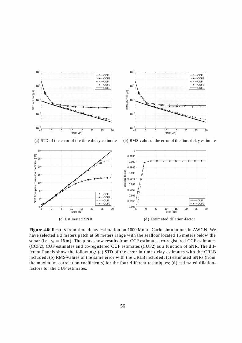
−5 0 5 10 15 20 25 3010

−3

10−2

10−1

100

101

SNR [dB]

ST

D o

f err

or [μ

s]

CCFCCF2CUFCUF2CRLB

(a) STD of the error of the time delay estimate

−5 0 5 10 15 20 25 3010

−3

10−2

10−1

100

101

SNR [dB]

RM

S o

f err

or [μ

s]

CCFCCF2CUFCUF2CRLB

(b) RMS-value of the error of the time delay estimate

−5 0 5 10 15 20 25 30−5

0

5

10

15

20

25

30

SNR [dB]

SN

R fr

om p

eak

corr

elat

ion

coef

ficie

nt [d

B]

CCFCCF2CUFCUF2

(c) Estimated SNR

−5 0 5 10 15 20 25 300.995

0.9955

0.996

0.9965

0.997

0.9975

0.998

0.9985

0.999

0.9995

1

SNR [dB]

Dila

tion−

fact

or

CUFCUF2

(d) Estimated dilation-factor

Figure 4.6: Results from time delay estimation on 1000 Monte Carlo simulations in AWGN. Wehave selected a 3 meters patch at 50 meters range with the seafloor located 15 meters below thesonar (i.e. z0 = 15m). The plots show results from CCF estimates, co-registered CCF estimates(CCF2), CUF estimates and co-registered CUF estimates (CUF2) as a function of SNR. The dif-ferent Panels show the following: (a) STD of the error in time delay estimates with the CRLBincluded; (b) RMS-values of the same error with the CRLB included; (c) estimated SNRs (fromthe maximum correlation coefficients) for the four different techniques; (d) estimated dilation-factors for the CUF estimates.

56

function differs from impulse signals and may start to limit the time delay accuracy forhigh SNRs.

In Figure 4.6(b) we see a clear bias in the time delay estimate using CCF, but onlya negligible bias when using CUF. However, the CCF has such a low overall perfor-mance, that an attempt to correct the bias is without interest. Figure 4.6(c) shows thatthe estimated SNR also significantly improves when using CUF relative to CCF. TheSNR calculated from the peak correlation value in the CCF deviates from the theoryalmost immediately, while the SNR calculated from CUF follows the theory relativelyclose. Figure 4.6(c) also shows that the results are improved by reducing the footprintshift effect. In Figure 4.6(d) we show that the estimate of the relative dilation-factorsagain is very stable, but now at a value of around 0.999. This is a moderate, but quiterealistic dilation factor for sidelooking sonars.

Figure 4.6 illustrates that for a sidelooking sonar geometry, the cross-correlation ba-sed time delay estimate is sub-optimum and will limit the accuracy of the relative depthestimate. The cross-uncertainty function better matches the signal model and improvesthe accuracy of the time delay estimate significantly. The standard deviation for highSNRs is reduced by an order of magnitude and a small bias present in the CCF esti-mate is removed. The estimated SNR from the peak correlation value is also increasedsignificantly, indicating a better match of the signals after CUF.

In synthetic aperture radar it has been suggested to eliminate the change of fre-quency in the signals received from different angles by trimming the spectra at theedges (Gatelli et al., 1994). This frequency change is the same as we have describedas a time dilation. The trimming is performed to ensure full overlap of the spectra at theexpense of a reduced bandwidth. This method works well for a theoretical spectrumwith zero amplitude in the stop band and at a flat response inside the passband. Howe-ver, due to the constructive and destructive interference of the scatterers, the receivedspectrum is a random realization of the transmitted spectrum. Figure 4.7 shows anexample of the variations in such a spectrum. From the properties of the Fourier trans-form we know that dilation or time scaling in time domain also dilates the spectrum(McClellan et al., 2003, pages 322-323). For a small patch of the spectrum we thereforesee an apparent frequency shift. This shift will not be addressed by cutting the spectraat the edges. However, the re-gridding performed in the CUF-algorithm will, as we cansee in Figure 4.7, remove most of this effect and increase the correlation between thesignals. An equivalent approach suggested by Gatelli et al. (1994) is to apply a range-and geometry-dependent frequency filter.

An alternative method of estimating the dilation in the received time signals is toestimate the shift in the spectra of the data and relate that to a dilation. This can beperformed by a center of mass estimation or by running a cross-correlation functiondirectly on the spectrum.

Another important question is the performance of the CCF and CUF estimators as afunction of dilation for a given SNR. In our sidelooking sensor geometry we have variedthe range (and thereby the dilation) for a fixed seafloor depth, and then performed aMonte Carlo simulation similar to the simulations presented above. Figures 4.8 and 4.9

57

4800 4850 4900 4950 5000 5050 51000

20

40

60

80

100

120

Pixels

Mag

nitu

de o

f the

spe

ctru

m

Array 1Array 2Array 2 after CUF

Figure 4.7: Zoom of an oversampled spectrum from one of the received time signals as a functionof data samples. The signal is selected from one of the realizations of the data presented in Figure4.6. The solid line is the spectrum for array one and the dot-dashed line the spectrum for arraytwo. The dashed line is the spectrum for array two after the interpolation performed in the CUFalgorithm (almost on top of the solid line).

show the results from such a study.The suppression angle in Figures 4.8 and 4.9 is defined as cos−1 (z0/r) where z0 =

15m and r is the range from receiver #2 to the center of the seafloor patch. Figure4.9 shows that CUF is superior for all suppression angles larger than five degrees. Inthis region and for this SNR, the dilation is the limiting factor when using the CCFestimator. From Figure 4.9(a) we see that at 35 degrees suppression angle, a CCF basedmethod gives a correlation coefficient of 0.5, equivalent to 0 dB SNR, while CUF hasa correlation coefficient corresponding to > 20dB. Note the effect of the co-registrationshowed in Figure 4.9(b). Using co-registrated CUF is important even for very high SNRsif the predicted SNR is to be used as a quality measure.

Figure 4.9(c) shows that CUF reduces the standard deviation of the error in the timedelay estimate between one and two orders of magnitude compared to CCF. From Fi-gures 4.9(c) and 4.9(d) we also see that the effect of scallop loss is strongly related bet-ween the dilation-factor estimate and the time delay estimate. The co-registration eli-minates the scallop loss and increases the estimated SNR significantly.

The results presented in this section indicate that CUF is a better time delay estimatorfor scenarios where the effect of dilation overshadows the effect of additive noise. Fora standard sidelooking sonar system this is almost always the case at near range. Onlyat far range where the dilation is less important, the CUF has the same performance asCCF. It should be noted that the effect of the dilation on CCF performance is a function

58

510152025303540450

0.02

0.04

0.06

0.08

0.1

0.12

0.14

0.16

Angle [deg]

Inte

rfer

omtr

ic d

elay

[ms]

CCFCCF2CUFCUF2Theoretical

(a) Time delay estimate

510152025303540450.993

0.994

0.995

0.996

0.997

0.998

0.999

1

1.001

Angle [deg]

Dila

tion−

fact

or

CUFCUF2Theoretical

(b) Estimated dilation-factor

Figure 4.8: Results from 1000 Monte Carlo simulations in AWGN. The SNR in the simulationsis 25 dB. We have selected a 3 meters patch at varying range, with the seafloor located 15 metersbelow the sonar (i.e. z0 = 15m). The plots show results from CCF estimates, co-registeredCCF estimates (CCF2), CUF estimates and co-registered CUF estimates (CUF2) as a functionof suppression angle. The different panels show the following: (a) theoretical and estimatedinterferometric time delay; (b) theoretical and estimated dilation-factor.

of the patch (or window) size. A larger patch will cause more decorrelation due todilation. However, a larger patch does also increase the accuracy in regions limited byadditive noise. As such, CUF provides the possibility to use larger patches, and therebybetter performance, than CCF.

As described in Section 3.1.3, the coherence-loss due to time-shift and time dilationcan be reduced by co-registrating the signals in ground-range. This method does notassume a linear dilation and hence is a higher order model than the CUF estimator,but it requires accurate knowledge of the geometry of the environment. A CUF-basedtime delay estimation can then be applied on the co-registrated data, in case there areany residual dilation left. In cases where the residual dilation is insignificant, CCF ispreferable to CUF due to simplicity and time-consumption.

4.5 Phase-differencing

In the SAR literature the interferometric delay is usually found by means of phase-differencing. The phase-difference is estimated using a maximum likelihood estimator(Hanssen, 2001, Page 92), which only differs from the complex cross-correlation in thatit is two-dimensional and that it does not shift the data. The phase-difference estimatoris a 2D zero-lag complex cross-correlation.

The phase-difference, θ, between two vertically separated receivers, is directly linked

59

510152025303540450.2

0.3

0.4

0.5

0.6

0.7

0.8

0.9

1

1.1

Angle [deg]

Cor

rela

tion

coef

ficie

nt

CCFCCF2CUFCUF2

(a) Maximum Correlation coefficient

51015202530354045−10

0

10

20

30

40

50

60

Angle [deg]

SN

R [d

B]

CCFCCF2CUFCUF2

(b) Estimated SNR

5101520253035404510

−4

10−2

100

102

104

Angle [deg]

ST

D o

f err

or [μ

s]

CCFCCF2CUFCUF2

(c) STD of the error of the time delay estimate

5101520253035404510

−7

10−6

10−5

10−4

10−3

10−2

10−1

Angle [deg]

ST

D o

f err

or

CUFCUF2

(d) STD of the error of the dilation estimate

Figure 4.9: Results from 1000 Monte Carlo simulations in AWGN. The SNR in the simulationsis 25 dB. We have selected a 3 meters patch at varying range, with the seafloor located 15 metersbelow the sonar (i.e. z0 = 15m). The plots show results from CCF estimates, co-registered CCFestimates (CCF2), CUF estimates and co-registered CUF estimates (CUF2) as a function of sup-pression angle. The different Panels show the following: (a) maximum correlation coefficients;(b) estimated SNR from the maximum correlation coefficients; (c) standard deviation of the errorin the time delay estimates; (d) standard deviation of the error in the dilation-factor estimates.

to the time delay estimate through the relation

τ =θ

2πf0, (4.28)

which is essentially the same as Equation 4.12. In principle, the time delay can be esti-mated for each sample-pair in the input data, but to reduce the noise we follow the SARliterature and introduce a maximum likelihood estimator over a local neighborhood.

60

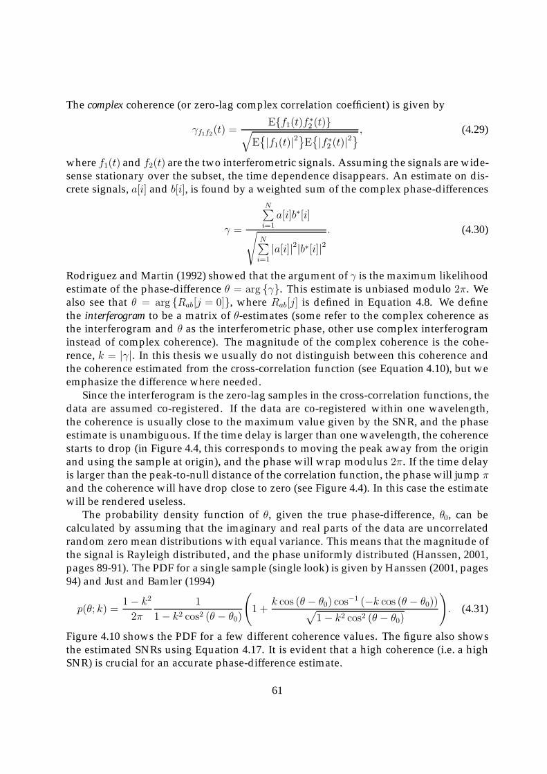
The complex coherence (or zero-lag complex correlation coefficient) is given by

γf1f2(t) =E{f1(t)f ∗

2 (t)}√E{|f1(t)|2}E{|f ∗

2 (t)|2} , (4.29)

where f1(t) and f2(t) are the two interferometric signals. Assuming the signals are wide-sense stationary over the subset, the time dependence disappears. An estimate on dis-crete signals, a[i] and b[i], is found by a weighted sum of the complex phase-differences

γ =

N∑i=1

a[i]b∗[i]√N∑i=1

|a[i]|2|b∗[i]|2. (4.30)

Rodriguez and Martin (1992) showed that the argument of γ is the maximum likelihoodestimate of the phase-difference θ = arg {γ}. This estimate is unbiased modulo 2π. Wealso see that θ = arg {Rab[j = 0]}, where Rab[j] is defined in Equation 4.8. We definethe interferogram to be a matrix of θ-estimates (some refer to the complex coherence asthe interferogram and θ as the interferometric phase, other use complex interferograminstead of complex coherence). The magnitude of the complex coherence is the cohe-rence, k = |γ|. In this thesis we usually do not distinguish between this coherence andthe coherence estimated from the cross-correlation function (see Equation 4.10), but weemphasize the difference where needed.

Since the interferogram is the zero-lag samples in the cross-correlation functions, thedata are assumed co-registered. If the data are co-registered within one wavelength,the coherence is usually close to the maximum value given by the SNR, and the phaseestimate is unambiguous. If the time delay is larger than one wavelength, the coherencestarts to drop (in Figure 4.4, this corresponds to moving the peak away from the originand using the sample at origin), and the phase will wrap modulus 2π. If the time delayis larger than the peak-to-null distance of the correlation function, the phase will jump πand the coherence will have drop close to zero (see Figure 4.4). In this case the estimatewill be rendered useless.

The probability density function of θ, given the true phase-difference, θ0, can becalculated by assuming that the imaginary and real parts of the data are uncorrelatedrandom zero mean distributions with equal variance. This means that the magnitude ofthe signal is Rayleigh distributed, and the phase uniformly distributed (Hanssen, 2001,pages 89-91). The PDF for a single sample (single look) is given by Hanssen (2001, pages94) and Just and Bamler (1994)

p(θ; k) =1− k2

2π

1

1− k2 cos2 (θ − θ0)

(1 +

k cos (θ − θ0) cos−1 (−k cos (θ − θ0))√

1− k2 cos2 (θ − θ0)

). (4.31)

Figure 4.10 shows the PDF for a few different coherence values. The figure also showsthe estimated SNRs using Equation 4.17. It is evident that a high coherence (i.e. a highSNR) is crucial for an accurate phase-difference estimate.

61

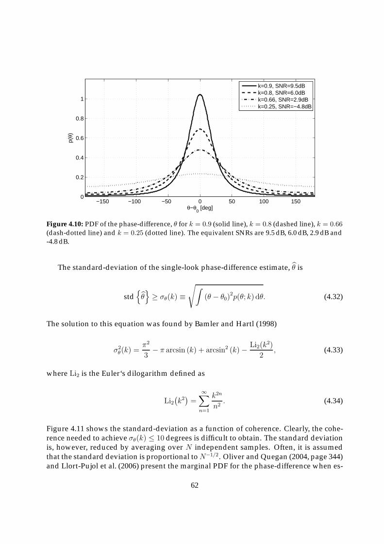
−150 −100 −50 0 50 100 1500

0.2

0.4

0.6

0.8

1

θ−θ0 [deg]

p(θ)

k=0.9, SNR=9.5dBk=0.8, SNR=6.0dBk=0.66, SNR=2.9dBk=0.25, SNR=−4.8dB

Figure 4.10: PDF of the phase-difference, θ for k = 0.9 (solid line), k = 0.8 (dashed line), k = 0.66(dash-dotted line) and k = 0.25 (dotted line). The equivalent SNRs are 9.5 dB, 6.0 dB, 2.9 dB and-4.8 dB.

The standard-deviation of the single-look phase-difference estimate, θ is

std{θ}≥ σθ(k) ≡

√∫(θ − θ0)

2p(θ; k) dθ. (4.32)

The solution to this equation was found by Bamler and Hartl (1998)

σ2θ(k) =

π2

3− π arcsin (k) + arcsin2 (k)− Li2(k

2)

2, (4.33)

where Li2 is the Euler‘s dilogarithm defined as

Li2(k2)=

∞∑n=1

k2n

n2. (4.34)

Figure 4.11 shows the standard-deviation as a function of coherence. Clearly, the cohe-rence needed to achieve σθ(k) ≤ 10 degrees is difficult to obtain. The standard deviationis, however, reduced by averaging over N independent samples. Often, it is assumedthat the standard deviation is proportional toN−1/2. Oliver and Quegan (2004, page 344)and Llort-Pujol et al. (2006) present the marginal PDF for the phase-difference when es-

62

10−6

10−5

10−4

10−3

10−2

10−1

0

2

4

6

8

10

12

14

16

1−k

σ θ(k)

[deg

]

Figure 4.11: Standard deviation of the phase-difference as a function of 1 − k, where k is thecoherence.

timated using a filter window of N independent samples

p(θ; k,N) =(1− k2)

N

2π

((2N − 2)!

((N − 1)!)222(N−1)

((2N − 1)K

(1−K2)N+ 12

cos−1 (−K) +1

(1−K2)N

)

+1

2(N − 1)

N−2∑r=0

Γ(N − 1

2

)Γ(N − 1

2− r) Γ(N − 1− r)

Γ(N − 1)

1 + (2r + 1)K2

(1−K2)r+2

),

(4.35)

where K = cos (θ − θ0) and Γ is the Gamma function (Rottmann, 1995). The standard-deviation becomes a function of coherence and number of independent samples.

std{θ}≥ σθ(k,N) ≡

√∫(θ − θ0)

2p(θ; k,N) dθ. (4.36)

Figure 4.12 shows the standard deviation as a function of coherence for a few filter-sizes.Clearly, σθ(k,N) does not scale as N−1/2. We define a scaling factor, S as

S = S(k,N) = − log (σθ(k))− log (σθ(k,N))

log (10), (4.37)

in such a way that σθ(k,N) = N−Sσθ(k). Notice that σθ(k, 1) = σθ(k). For a GaussianPDF, S is equal to 0.5. Figure 4.13 shows S as a function of k and N . In the usefulregion (k > 0.66) the reduction in standard-deviation as N is increased is larger than for

63

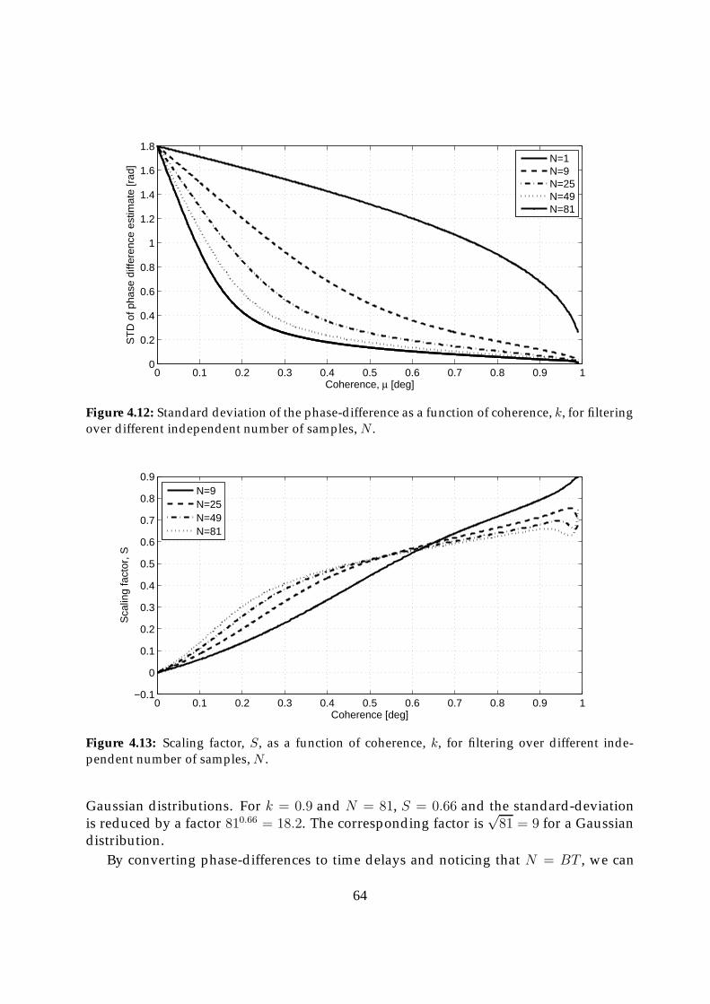
0 0.1 0.2 0.3 0.4 0.5 0.6 0.7 0.8 0.9 10

0.2

0.4

0.6

0.8

1

1.2

1.4

1.6

1.8

Coherence, μ [deg]

ST

D o

f pha

se d

iffer

ence

est

imat

e [r

ad]

N=1N=9N=25N=49N=81

Figure 4.12: Standard deviation of the phase-difference as a function of coherence, k, for filteringover different independent number of samples, N .

0 0.1 0.2 0.3 0.4 0.5 0.6 0.7 0.8 0.9 1−0.1

0

0.1

0.2

0.3

0.4

0.5

0.6

0.7

0.8

0.9

Coherence [deg]

Sca

ling

fact

or, S

N=9N=25N=49N=81

Figure 4.13: Scaling factor, S, as a function of coherence, k, for filtering over different inde-pendent number of samples, N .

Gaussian distributions. For k = 0.9 and N = 81, S = 0.66 and the standard-deviationis reduced by a factor 810.66 = 18.2. The corresponding factor is

√81 = 9 for a Gaussian

distribution.By converting phase-differences to time delays and noticing that N = BT , we can

64

−5 0 5 10 15 20 25 3010

−2

10−1

100

101

102

SNR ρ [dB]

ST

D o

f err

or [μ

s]

σc

σf

σi

σi (approx)

(a) N = 5

−5 0 5 10 15 20 25 3010

−4

10−3

10−2

10−1

100

101

102

SNR ρ [dB]

ST

D o

f err

or [μ

s]

σc

σf

σi

σi (approx)

(b) N = 81

Figure 4.14: Comparison of σc (solid line), σf (dashed line) and σi (dash-dotted line) as a functionof SNR, ρ. The dotted line shows σi under the approximation that the scaling factor S = 0.5.The left panel shows the case for N = 5 and the right panel for N = 81. In the right panel, σ i isindistinguishable from σf .

compare the three expressions for the standard deviation of the time delay estimatedirectly

σc(ρ,N,B) =

√3

π

1

B

1√N

√1

ρ+

1

2ρ2, (4.38)

σf (ρ,N, f0) ≈ 1

2πf0

1√N

√1

ρ+

1

2ρ2, (4.39)

σi(ρ,N, f0) =1

2πf0

1

NS

√∫(θ − θ0)

2p(θ; k(ρ)) dθ, (4.40)

where σi is the standard deviation of the time delay estimate based on the interfero-gram. Figure 4.14 compares the three quantities as a function of ρ using B = 30kHzand f0 = 100kHz. For N = 5, σc differs from σi even though the same data and almostthe same method is considered. The difference lies in the underlying assumption. InSection 4.1.3, σc and σf where based on constant deterministic signals in additive whiteGaussian random noise. In this section σi were based on a signals with Rayleigh dis-tributed magnitude and uniformly distributed phase (Hanssen (2001, pages 89-91); Justand Bamler (1994)). According to Hanssen (2001, page 95) the CRLB is a better model inthe presence of point scatterers while the marginal probability density function is bestsuited in the presence of speckle – the case for a general seafloor. As Figure 4.14 shows,σf is too optimistic in speckle statistics, while σi is too pessimistic on point scatterers.As we see in the right panel of Figure 4.14, the difference between σf and σf becomesnegligible for large estimation windows.

65

4.6 Model errors

In the previous sections we have considered signals in uncorrelated additive whitenoise. In general there are several other types of noise which limit the accuracy of timedelay estimation. Lurton (2002, page 103) groups the noise contribution into four

• Ambient noise – noise which originates from outside the system. It can be natural(e.g. waves or animals) or man-made (e.g. shipping).

• Self-noise – nose with originates inside the system. It can be caused by the suppor-ting platform (e.g. electrical interference) or by its own electronics (thermal noise).

• Reverberation – unwanted echoes generated by the sonars own signals.

• Acoustic interference – noise generated by other acoustic platforms in the vicinity.

Instead of grouping noise sources as Lurton (2002, page 103) does, we will try to give abrief mathematical description of different signal models. We start by reviewing signalsin uncorrelated additive white noise and then expand to more complicated scenarios.

4.6.1 Uncorrelated additive white noise

We assume that we receive two time series of a signal in uncorrelated additive whitenoise

f1(t) = s(t) + n1(t), (4.41a)f2(t) = s(t− δt) + n2(t), (4.41b)

The signals are time-shifted with δt and the SNR is the same in both time series. Uncor-related additive white noise is always present in measurement, but the SNR can varysignificantly. The simplest case is additive white Gaussian noise, which is assumed whenestablishing the CRLB of the time delay estimate (see Equation 4.18).

4.6.2 Baseline decorrelation

In general the signal-part of the received time series is not identical in the two timeseries. Increasing the interferometric baseline increases this difference

f1(t) = s1(t) + n1(t), (4.42a)f2(t) = s2(t− δt) + n2(t). (4.42b)

True baseline decorrelation is mismatched spectra (Lurton (2000); Hanssen (2001, page102)). This effect is irreversible and will lower the coherence and add noise to the es-timate unless the spectra are filtered (which will reduce the bandwidth). Geometricaldecorrelation (Gatelli et al., 1994) is simply a dilation of the signals inside the correla-tion window. As we showed in Section 4.3, the cross-uncertainty function is a betterestimator than the cross-correlation function in the presence of baseline decorrelation.

66

4.6.3 Multipath

In a reverberant environment the received signal is not a pure replica of the transmittedsignal. Reflections from medium boundaries and the roughness of the boundaries willspread the signal in time (Brekhovskikh and Lysanov, 1982, chapter 9). If the boundaryis moving (like the sea surface), a Doppler shift will be added to the scattered fieldand the signal spread in frequency (Brekhovskikh and Lysanov, 1982, chapter 9). Theseeffects can be incorporated in a transfer function, h(δt)

f1(t) = h(δt)� s(t) + n1(t), (4.43a)f2(t) = h(δt)� s(t− δt) + n2(t), (4.43b)

where � is the convolution operator. To resolve these ambiguities one can for examplebeamform the data in a given direction, use a parametric method to locate the echo oruse a generalized cross-correlation function with a filter in frequency domain (Knappand Carter, 1976). Time spread and frequency spread is treated in detail in wirelesscommunications (Benedetto and Biglieri, 1999, chapter 13).

4.6.4 Correlated noise

Uncorrelated noise and reverberant noise are both environment induced. Another noise-source is system self noise that may be correlated over the receiver array (Lurton, 2002,pages 116-117). This noise can be coherent and synchronized in the time series, es-pecially if the receivers have a common electrical system. The estimated time-shift isusually dominated by either the time-shifted signal, or the synchronized noise. The re-ceived time series are

f1(t) = s(t) + c(t) + n1(t), (4.44a)f2(t) = s(t− δt) + c(t) + n2(t), (4.44b)

where c(t) is the correlated noise. This noise (if it in fact is caused by the electricalsystem) can be estimated by running the system without transmitting a signal. It canthen be removed from the time series, although this can be challenging in practice.

4.6.5 Multiplicative noise

The medium (seawater) can also induce multiplicative noise from random fluctuations(Brekhovskikh and Lysanov (1982, chapter 10); Flatte et al. (1979, chapter 8)). One wayto model this is to introduce a random multiplicative component

f1(t) = α1(t)s(t) + n1(t), (4.45a)f2(t) = α2(t)s(t− δt) + n2(t). (4.45b)

In general α1(t) and α2(t) can be complicated and highly different, decorrelating thereceived time series. If the two time series have passed through the same medium, α1(t)

67

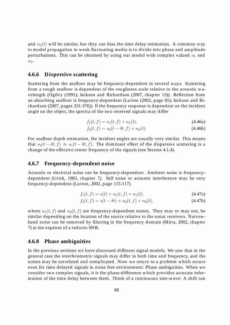
and α2(t) will be similar, but they can bias the time delay estimation. A common wayto model propagation in weak fluctuating media is to divide into phase and amplitudeperturbations. This can be obtained by using our model with complex valued α1 andα2.

4.6.6 Dispersive scattering

Scattering from the seafloor may be frequency-dependent in several ways. Scatteringfrom a rough seafloor is dependent of the roughness scale relative to the acoustic wa-velength (Ogilvy (1991); Jackson and Richardson (2007, chapter 13)). Reflection froman absorbing seafloor is frequency-dependent (Lurton (2002, page 65); Jackson and Ri-chardson (2007, pages 331-376)). If the frequency response is dependent on the incidentangle on the object, the spectra of the two received signals may differ

f1(t, f) = s1(t, f) + n1(t), (4.46a)f2(t, f) = s2(t− δt, f) + n2(t). (4.46b)

For seafloor depth estimation, the incident angles are usually very similar. This meansthat s2(t− δt, f) ≈ s1(t− δt, f). The dominant effect of the dispersive scattering is achange of the effective center frequency of the signals (see Section 4.1.4).

4.6.7 Frequency-dependent noise

Acoustic or electrical noise can be frequency-dependent. Ambient noise is frequency-dependent (Urick, 1983, chapter 7). Self noise or acoustic interference may be veryfrequency-dependent (Lurton, 2002, page 115-117).

f1(t, f) = s(t) + u1(t, f) + n1(t), (4.47a)f2(t, f) = s(t− δt) + u2(t, f) + n2(t), (4.47b)

where u1(t, f) and u2(t, f) are frequency-dependent noises. They may or may not, besimilar depending on the location of the source relative to the sonar receivers. Narrow-band noise can be removed by filtering in the frequency domain (Mitra, 2002, chapter7) at the expense of a reduces SNR.

4.6.8 Phase ambiguities

In the previous sections we have discussed different signal models. We saw that in thegeneral case the interferometric signals may differ in both time and frequency, and thenoises may be correlated and complicated. Now we return to a problem which occurseven for time delayed signals in noise free environment: Phase ambiguities. When weconsider two complex signals, it is the phase-difference which provides accurate infor-mation of the time delay between them. Think of a continuous sine-wave: A shift can

68

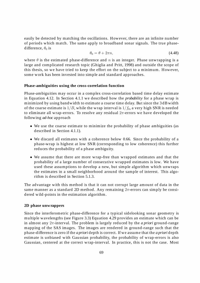
easily be detected by matching the oscillations. However, there are an infinite numberof periods which match. The same apply to broadband sonar signals. The true phase-difference, θ0 is

θ0 = θ + 2πn, (4.48)

where θ is the estimated phase-difference and n is an integer. Phase unwrapping is alarge and complicated research topic (Ghiglia and Pritt, 1998) and outside the scope ofthis thesis, so we have tried to keep the effort on the subject to a minimum. However,some work has been invested into simple and standard approaches.

Phase-ambiguities using the cross-correlation function

Phase-ambiguities may occur in a complex cross-correlation based time delay estimatein Equation 4.12. In Section 4.1.1 we described how the probability for a phase wrap isminimized by using bandwidth to estimate a coarse time delay. But since the 3 dB widthof the coarse estimate is 1/B, while the wrap interval is 1/f0, a very high SNR is neededto eliminate all wrap-errors. To resolve any residual 2π-errors we have developed thefollowing ad-hoc approach

• We use the coarse estimate to minimize the probability of phase ambiguities (asdescribed in Section 4.1.1).

• We discard all estimates with a coherence below 0.66. Since the probability of aphase-wrap is highest at low SNR (corresponding to low coherence) this furtherreduces the probability of a phase ambiguity.

• We assume that there are more wrap-free than wrapped estimates and that theprobability of a large number of consecutive wrapped estimates is low. We haveused these assumptions to develop a new, but simple algorithm which unwrapsthe estimates in a small neighborhood around the sample of interest. This algo-rithm is described in Section 5.1.3.

The advantage with this method is that it can not corrupt large amount of data in thesame manner as a standard 2D method. Any remaining 2π-errors can simply be consi-dered wild-points in the estimation algorithm.

2D phase unwrappers

Since the interferometric phase-difference for a typical sidelooking sonar geometry ismultiple wavelengths (see Figure 3.3) Equation 4.29 provides an estimate which can bein almost any 2π-interval. The problem is largely reduced by the a priori ground-rangemapping of the SAS images. The images are rendered in ground-range such that thephase-difference is zero if the a priori depth is correct. If we assume that the a priori depthestimate is unbiased with Gaussian probability, the probability of wrap-errors is alsoGaussian, centered at the correct wrap-interval. In practice, this is not the case. Most

69

of the samples are, in fact, wrap-free, but due to a slowly varying a priori depth, sharpelevated features will have wrap-errors. This means that samples with wrap-errors aregrouped together, but they should still be in minority. A standard 2D unwrapper worksvery well in such cases.

To solve the residual phase-wraps we have implemented a standard Goldstein‘sBranch cut algorithm as described in Ghiglia and Pritt (1998). We have not tested thismethod against other established methods, nor have we performed any thorough studyof the performance. However, the method works well in most cases. The exceptionis in the most challenging scenarios, which typically is large, complicated man-madeobjects with vertically features. In such cases we have performed a preliminary studyinto using bandwidth to resolve the phase ambiguities (see Section 8.3). We believe thatultra wideband signals reduce the need for advanced 2D unwrappers. Notice the simi-larity between such a method and the cross-correlation based method described in theprevious section.

4.7 Coherence estimation

In this chapter, as well as in most literature on interferometry, the focus has been on thetime delay estimate. The coherence estimate can be almost equally important (Synneset al., 2009; Midtgaard et al., 2009). In this section we give a short review of the statisticsof the coherence estimate.

The coherence can be defined as the magnitude of the complex coherence (see Equa-tion 4.29). Ideally, the estimate should be obtained using a very large number of ob-servations for each pixel-pair in the SAS images. In practical situations, each pixel-pairis observed only once and we assume ergodicity to exchange ensemble averages withspatial averages. This assumption leads to a maximum likelihood estimator over Nsamples

k =

∣∣∣∣∣∣∣∣∣∣N∑i=1

a[i]b∗[i]√N∑i=1

|a[i]|2|b∗[i]|2

∣∣∣∣∣∣∣∣∣∣. (4.49)

This estimator is clearly not unbiased. Two signals of uncorrelated noise should havek = 0, but Equation 4.49 will in this case result in a sum over vectors with random direc-tions, which clearly have an expectancy > 0 unless N → ∞. However, for completelycoherent signals in zero noise, Equation 4.49 will give out the expected answer of one. Ittherefore appears that the estimator is biased towards higher values for low coherenceand small estimation windows (Joughin and Winebrenner, 1994; Touzi et al., 1999).

Touzi and Lopes (1996) found that for N > 2, the probability density function ofthe coherence estimator can be expressed as a function of the true coherence, k0 and the

70

number of independent samples, N

p(k; k0, N) = 2(N − 1)(1− k2

)Nk0(1− k20

)N−22F1

(N,N, 1, k2k20

), (4.50)

where the hypergeometric function is defined as (Hanssen, 2001, page 94)

2F1

(N,N, 1, k2k20

)=

∞∑i=0

(N)i(N)i(1)i

(k2k20)i

i!, (4.51)

and the Pochhammer symbol is defined as

(N)i = N(N + 1)(N + 2) · · · (N + i− 1), (N)0 = 1. (4.52)

The expectation of k is derived as (Hanssen, 2001, page 96)

E{k;N} =Γ(N)Γ(3/2)

Γ(N + 1/2)3F2

(3/2, N,N,N + 1/2, 1, k2

)(1− k2

)N, (4.53)

where 3F2(3/2, N,N,N + 1/2, 1, k2) is the generalized hypergeometric function.Figure 4.15 shows the bias in the coherence estimate as a function of true coherence,

for different number of independent samples. We discard all time delay estimates withcoherence less than 0.66. For N = 81 and an estimated coherence of 0.66, the truecoherence is 0.63. This is only an error of 1 dB. For higher coherences, the bias getssmaller. However, we also try to estimate the coherence for samples where the timedelay estimate is useless. In Synnes et al. (2009) and Midtgaard et al. (2009) we presenttwo applications for sonar coherence mapping. Clearly, the bias can be important forsuch topics. It has been suggested to correct the biases coherence estimate, since thebias is analytically known (Touzi et al., 1999). Hanssen (2001, pages 96-98) shows thatat low coherence, the standard deviation of the coherence estimate is high. This meansthat a correction of the coherence can lead to unphysical values (e.g. the coherence canbe greater than unity).

71

0 0.1 0.2 0.3 0.4 0.5 0.6 0.7 0.8 0.9 10

0.1

0.2

0.3

0.4

0.5

0.6

0.7

0.8

0.9

1

k0

k

Bias freeN=5N=25N=81

Figure 4.15: The expectation value of k, as a function of the true coherence, k0 for a number ofdifferent samples in the estimator, N . The solid line shows the bias free estimate.

72

Chapter 5

Algorithms for depth estimation

In this chapter we describe how the methods from previous chapters are implemen-ted in an interferometric SAS processing chain. Estimation and use of relative seafloordepth can be found at several levels in SAS processing, each step being crucial for thesteps which follow. Thus, in order to make a high quality SAS bathymetry, all of thepreceding calculations have to be implemented as accurately as possible.

As mentioned in Chapter 1, a large portion of this thesis has consisted of contribu-ting to the development of the FOCUS toolbox (Hansen et al., 2005). FOCUS is a SASprocessing toolbox which takes raw sonar (or radar) data as input and generates a widevariety of outputs. Except for a few 1D simulations, all results presented in this thesisare generated using the FOCUS toolbox. Figure 5.1 shows a flowchart of the main pro-cessing chain in FOCUS. Processing steps involving relative depth estimation or use ofrelative depth estimates, are colored red in Figure 5.1. These can be grouped into threecategories:

• Ping-by-ping sidescan seafloor depth estimation (sidescan bathymetry)

• Use of estimated sidescan bathymetry in SAS processing

• SAS interferometry

5.1 Sidescan seafloor depth estimation

In this section we describe the implementation of relative depth estimation using singlebeam sidescan images. The sonar geometry can be found in Figure 3.1. Each of thereceivers in Figure 3.1 may represent a receiver array perpendicular to the page, butwhen the distinction is not important, we refer to them as receivers. Figure 5.2 showsan overview of the relative seafloor depth estimation algorithm.

The first step of sidescan bathymetry is to generate sidescan images. For both in-terferometric receiver arrays, each ping is dynamically focused (Soumekh, 1994, pages

73

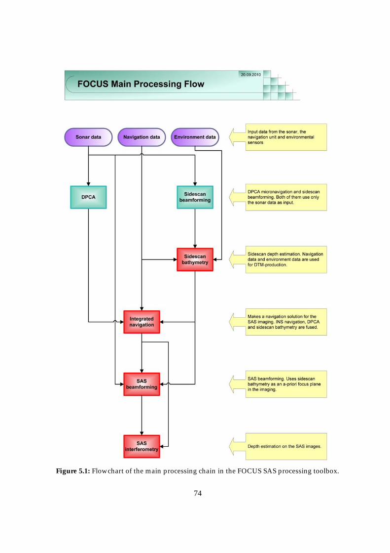
Figure 5.1: Flowchart of the main processing chain in the FOCUS SAS processing toolbox.

74

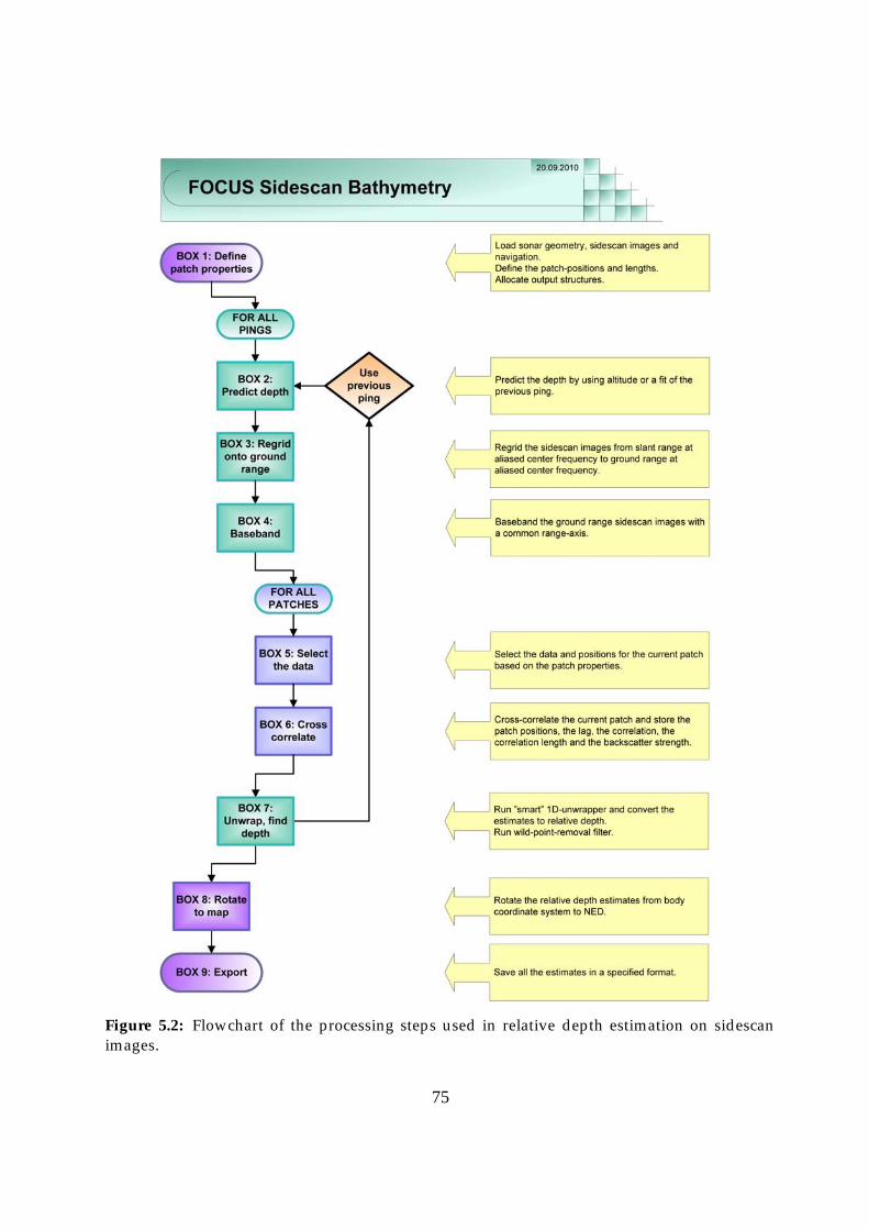
Figure 5.2: Flowchart of the processing steps used in relative depth estimation on sidescanimages.

75

196-209) in slant-range, forming a beam perpendicular to the transmitter-receiver ba-seline. The beams from the two receivers are not in general parallel, this only occurswhen the transmitter is positioned on a line between the two receivers. The origin ofthe beams can be the receivers, the PCA locations or the transmitter. The choice of ori-gin is not important, as long as the preferred choice is carried properly through theprocessing. We have chosen PCA locations as origin.

The beamforming results in two sidescan images, Isr1 [p, n] and Isr2 [p, n], where p is theping counter and n the sample counter along range. The subscript indicates receiver# and the superscript, sr indicates that the images are in slant-range. These images,together with the the sonar geometry and the sample distance, dr, are the main inputsto the depth estimation routine.

5.1.1 Re-gridding to ground-range

As we described in Section 3.1.3, we co-registrate the sidescan images by re-griddingthem onto an a priori seafloor. The seafloor is calculated using the relative depth esti-mates from the previous ping. For the first ping we kick-start the processing using a flatseafloor at the altimeter depth, and then re-estimate the ping using the estimated depthas a priori information. The same kick-starting is performed when the estimates fromthe previous ping are rendered invalid due to low coherence.

Let the two-way range from the transmitter to each sample in the sidescan imagesand back into the receiver be

rsr[n] = 2

√r2[n] +

(D

2

)2

, (5.1)

where r[n] = n · dr and D is the interferometric baseline between the transmitter andreceiver. This equation describes the dynamic focusing onto the PCA positions.

The range axes from the transmitter to the a priori seafloor and back to the receivers,are given by

rgr1 [m] =√y2[m] + z2[m] +

√(y[m]− y1)

2 + (z[m]− z1)2, (5.2a)

rgr2 [m] =√y2[m] + z2[m] +

√(y[m]− y2)

2 + (z[m]− z2)2. (5.2b)

Here y[m] = m · dy is a vector defined by a input parameter, dy, and z[m] is the a prioridepth corresponding to the positions y[m]. Figure 3.1 defines the receiver positions, y1,y2, z1, z2. The sidescan images are critically sampled in slant-range so we have to becareful to avoid undersampling in the new coordinate frame. For a flat a priori seafloor,dy = dr is sufficient, since the sampling frequency is dilated by cos θ in ground-rangerelative to slant-range (see Equation 3.12). For a general z[m], dy = dr may be insuffi-cient. By assuming a slowly varying a priori seafloor and decreasing dy by a small factor,undersampling is avoided for most practical geometries.

76

The re-gridding from slant-range to ground-range is implemented using a splineinterpolation (Kincaid and Cheney, 1991, pages 374-392). The sidescan images in slant-range are at aliased center frequency f0. We mix the slant-range data to baseband, inter-polate and mix the data up using the new ground-range sampling

Igr1 [p,m] = I{Isr1 [p, n] exp

(−j2πf0c

rsr[n]

): rsr[n] ⇒ rgr1 [m]

}exp

(j2πf0c

rgr1 [m]

), (5.3a)

Igr2 [p,m] = I{Isr2 [p, n] exp

(−j2πf0c

rsr[n]

): rsr[n] ⇒ rgr2 [m]

}exp

(j2πf0c

rgr2 [m]

), (5.3b)

where I{A[x] : x⇒ y} is an interpolation operator which interpolates A[x] from x ontoy, and j is the imaginary unit. The ground-range sidescan images are now at aliasedcenter frequency, f0, with non-linear range-axes (see Section 3.1.2).

We want to minimize interpolation errors in the subsequent processing, so we ba-seband the ground-range images (Hawkins, 1996, chapter 4). We have to decide on acommon range-axis for the basebanding and the natural choice is the average of rgr1 [m]and rgr1 [m].

rgr[m] =1

2(rgr1 [m] + rgr2 [m]). (5.4)

The basebanded ground-range sidescan images are given by

Igr,b1 [p,m] = Igr1 [p,m] exp

(−j2πf0c

rgr[m]

), (5.5a)

Igr,b2 [p,m] = Igr2 [p,m] exp

(−j2πf0c

rgr[m]

). (5.5b)

5.1.2 Cross-correlation of patches

For each ping of the ground-range sidescan images, a set of patches along range is se-lected. The locations of the patches and the number of samples in each patch is in-dependent parameters, and can be varied throughout the ping. Our default setting isone meter between each patch in ground-range, and a fixed patch-length of 3.2 meters.This gives us a regular griding of the estimates in an earth-fixed coordinate system and128 cosΦ individual samples in each correlation (for HISAS with 2.5 cm range resolu-tion), where Φ is the depression angle. The number of individual samples is largest atfar range, due to the scaling between ground-range and slant-range. It can be beneficialto increase the patch length at far range since baseline decorrelation is less of a problemand the SNR may be low.

For each of the selected patches we cross-correlate N complex samples from samplem1 to sample m2 (see Section 4.1)

Rgr,bI1I2

[p, j] = K

m2−m1+1−j∑m=m1

Igr,b1 [p,m+ j](Igr,b2 [p,m]

)∗, j = 0, 1, . . . , N − 1, (5.6)

77

where K is the normalization factor defined in Equation 4.9. The peak correlation valueis used to find the coarse pixel lag, jc

jc = argmaxj

{|RI1I2[j]|}, (5.7)

where the superscripts and the ping dependence are omitted for simplicity. The finedelay is given by Equations 4.11, 4.12 and 4.13, but since the input data are sampledregularly in spatial ground-range coordinates instead of in time, the equations look dif-ferent.

5.1.3 Unwrapping the sidescan bathymetry estimates

From the properties of the cross-correlation function of two time delayed signals, thephase should be zero at the true correlation peak. We have experienced from sidescanbathymetry estimates that the phase of the peak of the sampled cross-correlation func-tion does not strictly behave in accordance with this property. There are a number ofreasons why theory does not match experience

• The signals are sampled so the phase at the sampled peak differs from phase atthe true peak, unless the sampling frequency is infinite.

• The signals have noise on both the magnitude and the phase, so the selected peakmay be incorrect or the phase may be noisy.

• The signals are not only time delayed relative to each other, they are also dilated.

Figure 5.3 shows the phase distribution of the valid estimates for a simulated sea-floor with a non-linear trajectory and a varying topography. It shows that the distribu-tions are zero-mean, and that the spread of the phase distribution decreases when thecross-correlation function is upsampled (see Section 4.1.1). Note that if the data is ade-quately sampled one can upsample the cross-correlation function rather than the inputsidescan images.

Figure 5.4 illustrates how the distribution is widened when the bathymetry of theseafloor becomes more challenging. This is due to an increased dilation and a less ac-curate a priori seafloor depth estimate. Comparison of the simulated data in Figure 5.3with the experimental data in Figure 5.4 also reveals the widening of the phase distri-bution due to noise.

From Figures 5.3 and 5.4, and as mentioned in Section 4.1.1, 2π-wrap errors willoccur even for cross-correlation based methods. These wrap-errors occurs rarely, but arerandomly distributed throughout the sidescan image. A simple 1D unwrapper (Ghigliaand Pritt, 1998, pages 16-26) will successfully unwrap most of these samples, but in afew cases it can contribute to a large error: If the unwrapper is run across a shadowregion or across pixels with low coherence, all subsequent samples for that ping maybe wrapped out of the correct 2π-interval. Figure 5.5 shows an example where this has

78

−100 0 1000

0.1

0.2

0.3

0.4

0.5

Phase [deg]

Occ

urre

nce

(a) Critical sampling

−100 0 1000

0.1

0.2

0.3

0.4

0.5

Phase [deg]

Occ

urre

nce

(b) Oversampling with a factor of 10

Figure 5.3: Distribution of the phases of the peak of the cross-correlation functions in sidescanbathymetry, for 1000 simulated pings with 150 patches each. Pixels with a correlation valuebelow 0.66 have been discarded. The bathymetry is slowly varying over the scene. The leftpanel shows the results when the sidescan data are critically sampled, while the right panelshows the results when the sidescan data are oversampled with a factor of ten in the re-griddingto ground-range. The solid lines indicate 90% of the data and the dashed line 99%.

−100 0 1000

0.1

0.2

0.3

0.4

0.5

Phase [deg]

Occ

urre

nce

(a) Flat seafloor

−100 0 1000

0.1

0.2

0.3

0.4

0.5

Phase [deg]

Occ

urre

nce

(b) Heavy topography

Figure 5.4: Distribution of the phases of the peak of the cross-correlation functions in sidescanbathymetry, for 1000 pings with 200 patches each. Pixels with a correlation value below 0.66have been discarded. The data are real data collected using HISAS. The left panel shows theresults for an approximate flat seafloor, while the right panel shows the results for a seafloorwith heavy topography. The solid lines indicate 90% of the data and the dashed line 99%.

79

40 60 80 100 120 140−0.5

0

0.5

1

1.5

Patch number

δy/c

/2f 0gr

Figure 5.5: Normalized lag, δy/c/2fgr0 for a ping of real data collected with HISAS. The patch

numbers are increasing with range and are spaced with one meter separation in ground-range(e.g. patch 100 is at 100 meters ground-range). The raw estimates are showed with dots. Theestimates unwrapped with a standard 1D unwrapper are shown with squares and the estimatesunwrapped with our local 1D unwrapper are shown with circles. Notice that patch 148 and 149originally seem to be in the wrong 2π-interval.

happened on real data using HISAS. All the estimates from patch 112 and upward arewrapped up to a normalized lag of approximately one. In this case, the correct wrapinterval is closer to zero. The error is caused by the region of invalid samples frompatch 102 to patch 111. This is a region with shadow in the sidescan images where thecorrelation values are below 0.66. The geometry changes through the shadow and it isnot possible to know where to continue the unwrapping.

If we use phase differencing on the ground-range sidescan images instead of cross-correlations, the phases would vary smoothly with large spatial correlation between thesamples. However, when we cross-correlate and select the peak of the correlation func-tion, the phases will be zero-mean with no spatial correlation. In other words: a singlesample will with high probability be in the correct 2π-interval and it will be uncorrela-ted to the neighboring samples. The wrapped samples will be few, and they will occurrandomly in the data. We therefore define a new local unwrapper which unwraps eachsample to a local median of valid pixels

δy[m] = U{δy[m],Mu{δy[m− u : m+ u]}}, (5.8)

where u is a small number of samples, U{x, y} unwraps the estimate x onto the samewrap-interval as y andMu{δy[m− u : m+ u]} is the median value of the u valid samplesclosest to the sample m in the interval [m− u,m+ u] (exluding m itself). This means for

80

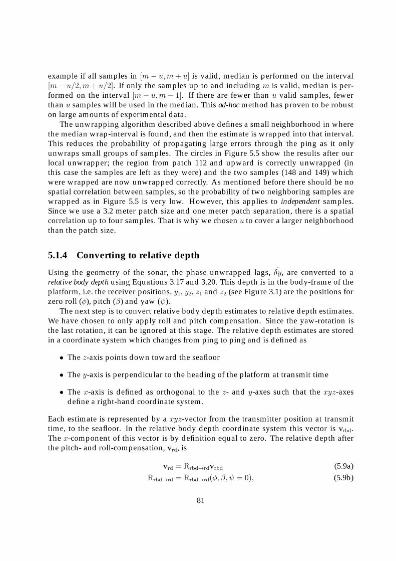
example if all samples in [m− u,m+ u] is valid, median is performed on the interval[m− u/2, m+ u/2]. If only the samples up to and including m is valid, median is per-formed on the interval [m− u,m− 1]. If there are fewer than u valid samples, fewerthan u samples will be used in the median. This ad-hoc method has proven to be robuston large amounts of experimental data.

The unwrapping algorithm described above defines a small neighborhood in wherethe median wrap-interval is found, and then the estimate is wrapped into that interval.This reduces the probability of propagating large errors through the ping as it onlyunwraps small groups of samples. The circles in Figure 5.5 show the results after ourlocal unwrapper; the region from patch 112 and upward is correctly unwrapped (inthis case the samples are left as they were) and the two samples (148 and 149) whichwere wrapped are now unwrapped correctly. As mentioned before there should be nospatial correlation between samples, so the probability of two neighboring samples arewrapped as in Figure 5.5 is very low. However, this applies to independent samples.Since we use a 3.2 meter patch size and one meter patch separation, there is a spatialcorrelation up to four samples. That is why we chosen u to cover a larger neighborhoodthan the patch size.

5.1.4 Converting to relative depth

Using the geometry of the sonar, the phase unwrapped lags, δy, are converted to arelative body depth using Equations 3.17 and 3.20. This depth is in the body-frame of theplatform, i.e. the receiver positions, y1, y2, z1 and z2 (see Figure 3.1) are the positions forzero roll (φ), pitch (β) and yaw (ψ).

The next step is to convert relative body depth estimates to relative depth estimates.We have chosen to only apply roll and pitch compensation. Since the yaw-rotation isthe last rotation, it can be ignored at this stage. The relative depth estimates are storedin a coordinate system which changes from ping to ping and is defined as

• The z-axis points down toward the seafloor

• The y-axis is perpendicular to the heading of the platform at transmit time

• The x-axis is defined as orthogonal to the z- and y-axes such that the xyz-axesdefine a right-hand coordinate system.

Each estimate is represented by a xyz-vector from the transmitter position at transmittime, to the seafloor. In the relative body depth coordinate system this vector is vrbd.The x-component of this vector is by definition equal to zero. The relative depth afterthe pitch- and roll-compensation, vrd, is

vrd = Rrbd→rdvrbd (5.9a)Rrbd→rd = Rrbd→rd(φ, β, ψ = 0), (5.9b)

81

where φ and β are the roll and pitch of the platform at transmit time and Rrbd→rd(φ, β, ψ)is the rotation matrix from body to the roll- and pitch-compensated coordinate system.These broadside depth estimates are a suitable intermediate data format since they canbe used for ping based processing and easily converted into earth-fixed coordinate sys-tems. Figure 5.6 shows an example of the ping-based relative depth estimates and amosaic into a local earth-fixed coordinate system. Notice that the platform depths areadded to the relative depths in the mosaic. Also notice that estimator at long range suc-cessfully estimates the seafloor depth even when it is above the sonar (the areas withnegative depth in Figure 5.6).

In Figure 5.6(a) there are blank areas where data seem to be missing. These are areaswhere the correlation coefficients are less than the threshold. All sidescan bathymetryestimates in this thesis are presented with a threshold of 0.66 (approximately equal to aSNR of 3 dB). Invalid samples typically appears in the following regions:

• In close-range regions the baseline decorrelation effect can reduce the correlationcoefficients

• In far-range regions the SNR may drop due to lack of signal energy

• In shadow regions caused by topography, there is no signal energy

• In areas with interference and multipath the correlation may drop (although so-metimes the interference can be coherent between the interferometric receivers)

5.1.5 Sound speed correction

One of the effects which makes sidelooking depth estimation more challenging thandownlooking depth estimation (e.g. single beam echo sounding and multibeam echosounding (Lurton, 2002, chapter 8)) is the effect of a vertically varying sound speedprofile. A signal traveling through a medium with a varying sound speed will notfollow a straight path (Brekhovskikh and Lysanov, 1982, Pages 33-35). Only directlyvertical rays will be straight. The degree of ray bending increases with how close youget to horizontal, so a sonar which looks 200 meters to the side in 20 meters water depthwill be much more susceptible to this effect than a sonar which only sees 45 degrees andsteeper. Sound velocity correction is common to do for high precision mapping sonars(Lurton, 2002, pages 278-281)

The effect of ray-bending is that the position and depth of the estimate both can beincorrect. What we really measure with the interferometer is the incident angle of thereflection into the sonar, along with the travel time. These two values can be found fromthe estimated depths and are sufficient to correct for ray-bending. We have chosen touse a standard constant gradient raytracer (Brekhovskikh and Lysanov (1982, Pages 37-38); Synnes (2008)) as a correction algorithm. The principle is to divide the sound speedprofile into a number of segments. Within each segment a constant gradient is assumed.

82

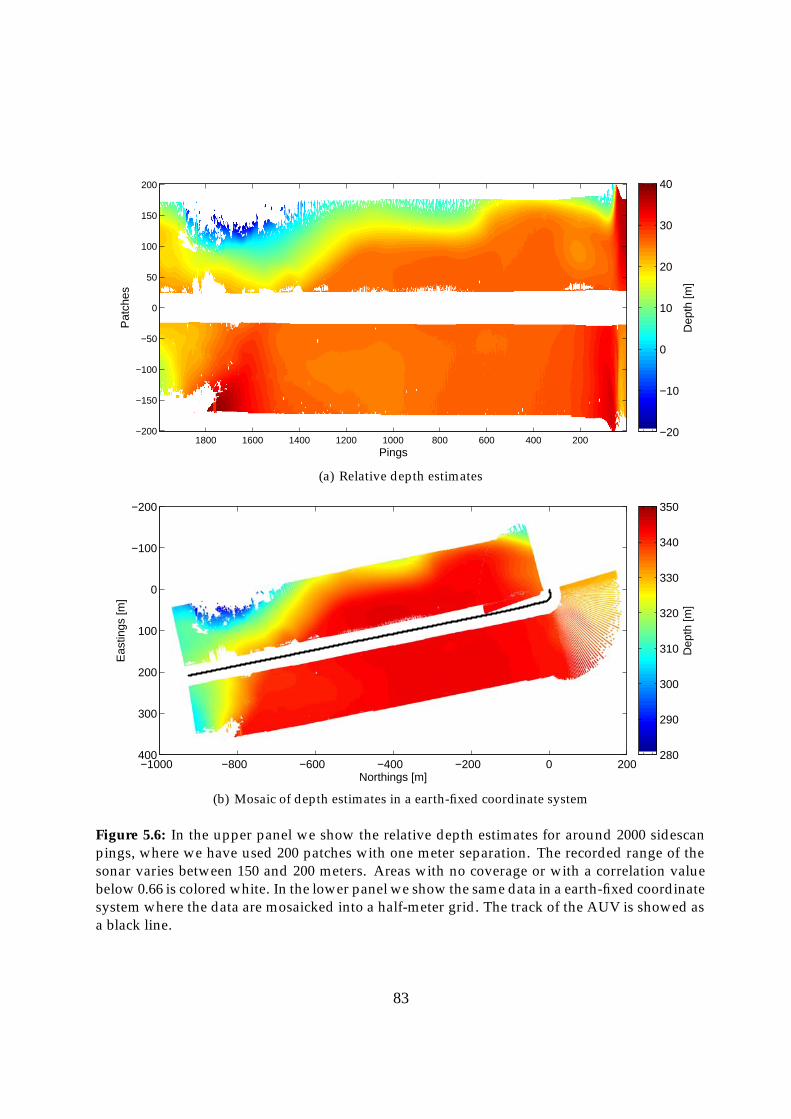
Pings

Pat

ches

20040060080010001200140016001800−200

−150

−100

−50

0

50

100

150

200

Dep

th [m

]

−20

−10

0

10

20

30

40

(a) Relative depth estimates

Northings [m]

Eas

tings

[m]

−1000 −800 −600 −400 −200 0 200

−200

−100

0

100

200

300

400

Dep

th [m

]

280

290

300

310

320

330

340

350

(b) Mosaic of depth estimates in a earth-fixed coordinate system

Figure 5.6: In the upper panel we show the relative depth estimates for around 2000 sidescanpings, where we have used 200 patches with one meter separation. The recorded range of thesonar varies between 150 and 200 meters. Areas with no coverage or with a correlation valuebelow 0.66 is colored white. In the lower panel we show the same data in a earth-fixed coordinatesystem where the data are mosaicked into a half-meter grid. The track of the AUV is showed asa black line.

83

The ray within such a segment will then follow a circular arc (Ziomek, 1985, Pages 220-240). The algorithm consists of estimating an incident angle from the uncompensateddepth estimates

Φ(r) = tan−1{z(r),

√r2 − z2(r)

}, (5.10)

where z is the uncompensated depth estimate and r the range. A ray is then sent outfrom the sonar in the Φ(r) direction and traced through the different segments until ithas traveled a length r. This results in a new position and depth on the seafloor.

Figure 5.7(a) shows an example dataset where we have compared depth estimatesbefore and after sound speed correction. Before correction there is a pronounced trendin the data as a function of range. The seafloor depth seems to bend downward on bothsides of the sonar. This is a typical result of uncompensated sound speed variations. Inthe middle panel we have removed the artificial trend by sound speed correcting theestimates. There is a difference of up to five meters, which is significantly larger thanthe precision of the depth estimates. Figure 5.7(b) shows that the sound speed profilefor this dataset has a relatively strong variation.

5.1.6 Exporting sidescan bathymetry digital terrain maps

The sidescan bathymetry estimates are a vital component in the SAS processing andhave to be easily accessible. In addition, the estimates are an excellent product for fast,low resolution assessment of the seafloor depth. We have therefore implemented threeexport formats

• MATLAB .mat format (Mat, 2010) for internal use in the processing

• Kongsberg .all format (Tri, 2008) for viewing with Kongsberg products

• Triton .xtf format (EMD, 2010) for viewing with Triton software

The exporting to .all and .xtf is performed in a stand-alone routine which reads theinternal format and converts it to appropriate form. This makes it easy to extend toother formats if needed.

The details of the exporting is fairly straightforward, but there are a few remarks:Navigation information has to be provided along with the lever-arm from the naviga-tion reference location to the transmitter. Since there is one sonar on each side there aretwo separate lever-arms and it is convenient to store the estimates from each side in itsown file. The xyz-estimates, the reflectivity and the coherence should all be stored inthe file to provide a quality estimate with the measurement.

In order to produce a proper digital terrain map (DTM) one should correct for en-vironmental effects like tide and surface waves (Ambrose and Geneva (1995); de Jonget al. (2002, pages 12-39)). This should be done in an external software. The same goesfor the geo-referencing of the data. A multitude of post-processing softwares designedfor these purposes exist already, but it is outside the scope of this thesis to evaluatethem.

84

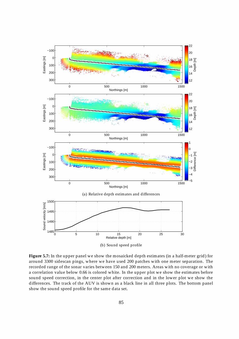
Northings [m]

Eas

tings

[m]

0 500 1000 1500

−100

0

100

200

300

Dep

th [m

]

12

14

16

18

20

22

Northings [m]

Eas

tings

[m]

0 500 1000 1500

−100

0

100

200

300

Dep

th [m

]

12

14

16

18

20

22

Northings [m]

Eas

tings

[m]

0 500 1000 1500

−100

0

100

200

300

Diff

eren

ce [m

]

−5

−4

−3

−2

−1

0

1

(a) Relative depth estimates and differences

0 5 10 15 20 25 301485

1490

1495

1500

Relative depth [m]

Sou

nd v

eloc

ity [m

/s]

(b) Sound speed profile

Figure 5.7: In the upper panel we show the mosaicked depth estimates (in a half-meter grid) foraround 3300 sidescan pings, where we have used 200 patches with one meter separation. Therecorded range of the sonar varies between 150 and 200 meters. Areas with no coverage or witha correlation value below 0.66 is colored white. In the upper plot we show the estimates beforesound speed correction, in the center plot after correction and in the lower plot we show thedifferences. The track of the AUV is shown as a black line in all three plots. The bottom panelshow the sound speed profile for the same data set.

85

5.2 Use of depth estimates in SAS processing

In the previous section we discussed how we have implemented relative depth estima-tion using sidescan images. The method provided us with fast and robust knowledge ofthe bathymetry, with a resolution of a few meters. Although this is a valuable productfor rapid environmental assessment (REA), it is even more important as a priori infor-mation in the SAS processing. The depth estimates provides the correct geometry forintegration of micronavigation estimates and for imaging. The coherence of the sides-can bathymetry estimates is an estimate of the sonar SNR, which is very important forquality assessment.

5.2.1 Integration of micronavigation estimates

The HUGIN AUV has a high-grade inertial measurement unit (IMU) with a numberof aiding sensors integrated in an error-state Kalman filter (Jalving et al., 2003). Theattitudes estimates from the integrated navigation system (INS) are accurately enoughfor SAS imaging. However, the INS position-estimates are limited by a poor along-track velocity (surge) estimate. Synthetic aperture sonar processing, on the other hand,requires extremely accurate cross-track motion (sway) estimates. Depending on thetype of error, the demand may be as high as better than λ/16 position-error over thesynthetic aperture (Cutrona, 1975). By combining measurements using DPCA with thenavigation solution from the integrated navigation system, the accuracy of both surgeand sway may be improved to a level where defocus is avoided (Bellettini and Pinto,2002).

In order to combine DPCA surge and sway measurements with the INS navigation-solution the depression angle Φ (or equivalently: the relative depth), has to be knownfor each ping and each DPCA patch. In principle, a depth estimate should be an averageover all depths within the sonars beamwidth and within the patch interval, weightedby the reflectivity. In order to achieve this all depth estimates have to be consideredfor each ping. We have implemented and tested this approach, but found that it wasunpractical due to the time consumption.

A fast approximation is to consider each ping separately by interpolating the relativebody depth estimates, vrbd, into the appropriate range values. The depression angle, Φis then defined as

Φ =

⎧⎨⎩ arcsin(

vrbd

|vrbd| · z)

: starboard

π arcsin(

vrbd

|vrbd| · z)

: port,(5.11)

where z is the unit-vector [0,0,1] and Φ is the angle between the vector to the seafloorand the xy body plane of the AUV. A depression angle, Φ = π/2 means a directiondirectly down in the body coordinate system of the AUV.

In addition to the depression angle, the along-track slope of the seafloor relative tothe body coordinate system of the AUV is used in the DPCA integration. The slope is

86

estimated for each patch and each ping by a simple weighted linear fit over the neigh-boring pings which are within the element beamwidth. Either reflectivity or coherenceor a combination of both can be used as weights.

5.2.2 Focus plane for imaging

It is well known that synthetic aperture images defocus if the focus plane is incorrectand the sensor path is non-linear (Jakowatz et al. (1996, pages 176-186); Hansen et al.(2009)). For a linear path, cylindrical symmetry ensures that the two-way travel pathis independent of depression angle, Φ. For a non-linear path, the travel path becomesa function of Φ, which means that the coherent summation of pings can decorrelate ifΦ is incorrect. It has been claimed (Pinto, 2003) that the integration of micronavigationestimates into the navigation solution will compensate for errors in the focus plane, butwe believe that this only applies in special cases: In general, both the navigation andthe focus plane have to be known.

In the FOCUS processing suite there are two different beamformers: A time-domaininterpolation beamformer (Johnson and Dudgeon, 1993, pages 112-119) which works onany form of trajectory and generates SAS images in ground-range, and a wavenumberalgorithm (Soumekh, 1999, pages 198-206) which is much faster, but demands close tolinear trajectories and generates slant-range images. The sidescan bathymetry depthestimates are used as a priori input to both algorithms, but the actual implementationsdiffer strongly.

Depth plane for time-domain imaging

The time-domain interpolation beamformer migrates data from the sensor position gi-ven by the navigation system, down onto an earth-fixed focus plane. The plane is madefrom sidescan bathymetry estimates by mosaicking the estimate into the same coordi-nate system as defined by the navigation solution. Mathematically, we transform eachroll- and pitch-compensated sidescan bathymetry estimate, vrd, into the earth-fixed na-vigation coordinate system as following

vxef = vxrd cos (ψ) + vyrd sin (ψ) + wxef , (5.12a)

vyef = vyrd cos (ψ)− vxrd sin (ψ) + wyef , (5.12b)

vzef = vzrd + wxef , (5.12c)

where vxyzrd are the xyz-components of vrd, wef the 3D position-vector of the transmitterand vef are the depth estimates in the earth-fixed coordinate system. These estimates arescatter points (i.e. they are unevenly distributed in x and y) and cannot be used directlyin the imaging.

The time-domain beamformer migrates the sonar data to a regular grid in x and y.The focus plane is therefore divided into rectangular cells with size given by the xy grid-spacing, and the depth for each cell is estimated as a weighted average of a number of

87

samples in vef . We have chosen to use a truncated Gaussian spatial weighting combinedwith coherence weighting. The size of the truncated Gaussian disk is a processing para-meter. If it exceeds the cell-size in any dimension, a single sidescan bathymetry depthestimate will contribute to multiple z-estimates. This is a simple way of smoothing thedata.

Slant-range directions for wavenumber imaging

The wavenumber algorithm beamforms sonar data in slant-range rather than ground-range, and does not use seafloor depth information. However, the beamforming as-sumes a linear sensor-trajectory, so we have to motion-compensate the data in advance(Callow et al., 2009). The motion-compensation transforms data collected on a non-linear track to data corresponding to data collected on a linear track. This is in fact alow-resolution time-domain beamforming, which needs seafloor depth information asinput.

There are a number of different approaches to the motion-compensation. In wide-beam motion-compensation seafloor depth, not only as a function of range, but also asa function of horizontal angle are taken into account. In narrow-beam motion-compen-sation it is assumed that the broadside beam is representative for the full horizontalbeamwidth. We have chosen a narrow-beam motion-compensation since it is muchfaster than the wide-beam. With 32 elements in each HISAS receiver array, this meansthat the depth is only estimated inside 1/32-part of the actual footprint of the elementdata.

Ideally we should use multiple sidescan bathymetry estimates as depth informationfor a single ping. This means making an earth-fixed depth map (as described in theprevious section) and ray-tracing the beams of each element down onto the depth map.This method uses all available information, but it is very time-consuming. We have im-plemented this method as an option, but use a simpler approach as default. Sidescanbathymetry estimates from a single ping is used to predict the depths for a single ping inthe motion-compensation. Missing estimates (due to too low coherence) are interpola-ted from neighboring ranges. Only in the case where the sidescan bathymetry estimatesfor an entire ping are missing, we copy information from neighboring pings.

5.3 SAS interferometry

Even though SAS interferometry is the end-product in the interferometric processing, itis also one of the easier steps to describe. Most of the processing is based on the sameprinciples as the sidescan bathymetry algorithm. In particular, the conversion fromdelay to relative depth, the sound speed correction and the exporters are all more or lessidentical to the methods described in Section 5.1. However, other parts are significantlydifferent. In this section we will discuss the details of the co-registration of the SASimages, the estimation of the interferogram, and the unwrapping of the interferogram.

88

We will also show how we can iteratively estimate the SAS bathymetry by using the firstestimate as input to a new co-registration step. This potentially increases the coherenceand the accuracy of the estimated bathymetry.

5.3.1 Co-registration

Co-registration of synthetic aperture images is in general a complicated problem. Aswe mentioned in Section 3.1.4, a method commonly used in SAR is to identify com-mon features in the SAR images and interpolate one of the images to match the other(Fornaro and Franceschetti, 1995). Usually, a warping function describing shift, dilationand rotation is calculated from a set of control points or distinctive image features (Honget al. (2006)); Jakowatz et al. (1996, Pages 293-298)). This is necessary in repeat-pass in-terferometry (Hanssen, 2001, page 2). For a single-pass interferometer like HISAS, theinterferometric images are not rotated relative to each other, so instead of a warpingfunction we use 1D interpolations along range.

Time-domain beamformed images are generated directly in ground-range and donot need to be co-registered. Slant-range SAS images are defined in the same coordinatesystem as sidescan images, so we can use the same mathematics as in Section 5.1.1.The main difference is that the data is motion-compensated to a straight-line and PCA-corrected to appear as collected from the PCA positions of the interferometric receivers.This means that rsr[n] = n · dr, and Equation 5.2 should be replaced by

rgr1 [m] = 2

√(y[m]− yPCA

1 )2+ (z[m]− zPCA

1 )2, (5.13a)

rgr2 [m] = 2

√(y[m]− yPCA

2 )2+ (z[m]− zPCA

2 )2, (5.13b)

with yPCA1 = y1/2, yPCA

2 = y2/2, zPCA1 = z1/2 and zPCA

2 = z2/2. Figure 3.1 definesthe receiver positions y1, y2, z1, z2. The actual interpolation is the same as in Equation5.3 and the basebanding is given by Equation 5.5. The a priori seafloor estimates z[m]for each y[m] is found by defining an earth fixed coordinate system and applying themethods described in Section 5.2.2.

5.3.2 Estimating the interferogram

Once we have co-registered the images in ground-range, the estimation of the inter-ferogram is straightforward. We implement the maximum likelihood estimator of thecomplex coherence described in Equation 4.29 (see Section 8.1). The argument of thecomplex coherence is the interferogram, while the magnitude is the coherence. Notethat the frequency used when converting the interferogram to relative depth is the sca-led ground-range frequency (see Section 5.1.2).

89

5.3.3 Unwrapping the interferogram

Since the interferogram is wrapped modulo 2π, we have to unwrap the phases beforewe can estimate the relative depth. The actual implementation follows the descriptionin Section 4.6.8. As we discussed, the phase wraps are minimized by the ground-rangeco-registration, and the residual unwrapping is performed using a standard Goldstein‘sBranch cut algorithm as described in Ghiglia and Pritt (1998).

5.3.4 Generating SAS images using SAS bathymetry

In this section we have described how FOCUS relies on relative seafloor depth esti-mates, made using the sidescan bathymetry algorithm. The performance of precedingmethods rely on the accuracy of these estimates. SAS bathymetry is an estimate ofthe relative seafloor depth with much higher horizontal resolution than sidescan ba-thymetry. An iterative scheme can therefore be made by using SAS bathymetry as animproved a priori input to the SAS processing. This can be implemented throughout theprocessing chain, but we have chosen to focus on an improved estimation of a focusplane. An improved a priori input will provide a better co-registration and less occur-rence of 2π phase wraps. This again will give us depth estimates with better precisionand accuracy. Figure 5.8 shows the interferograms using flat seafloor, sidescan bathy-metry and SAS bathymetry as a priori focus plane. The results are generated using apoint scatter simulation of a bumpy seafloor (see the upper left panel of Figure 5.8).The interferograms get closer to zero, the better the a priori depth information is. Sincethe simulated seafloor is very bumpy, there is still a residual phase-difference left in theinterferogram after iterative SAS processing (see the lower right panel of Figure 5.8).

Figure 5.9 shows the SNR calculated from the estimated coherence (using Equation4.17). The figure illustrates the increase in SNR due to improved co-registration. Theaverage improvement by using iterative SAS with SAS bathymetry as focus plane ins-tead of a flat seafloor (which has maximum 1 meter error), is in this case 4 dB. In mostrealistic cases, the seafloor depths are sufficiently smooth so sidescan bathymetry willbe accurate enough as depth information. However, on rock-formations or large man-made objects iterative SAS may significantly improve the results.

90

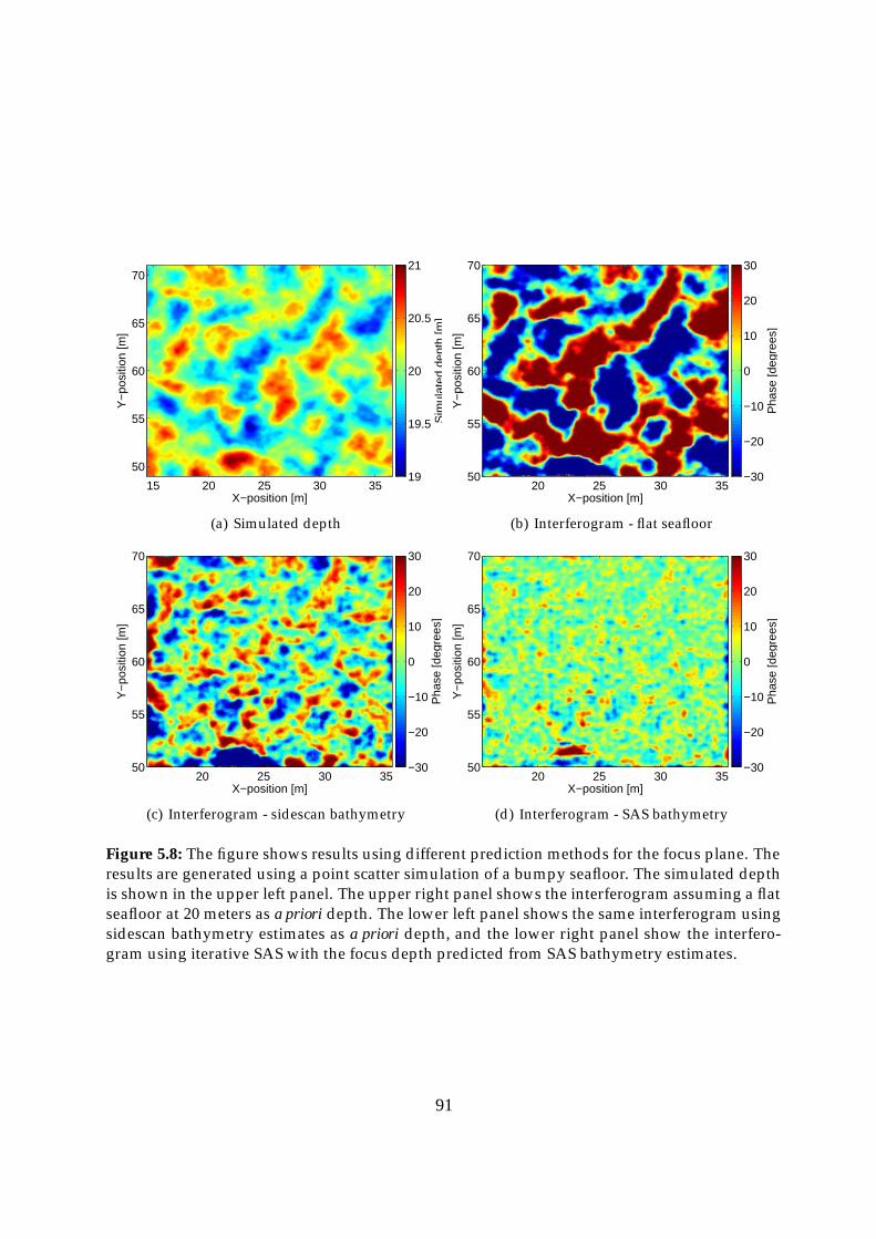
X−position [m]

Y−

posi

tion

[m]

15 20 25 30 35

50

55

60

65

70

Sim

ulat

ed d

epth

[m]

19

19.5

20

20.5

21

(a) Simulated depth

X−position [m]

Y−

posi

tion

[m]

20 25 30 3550

55

60

65

70

Pha

se [d

egre

es]

−30

−20

−10

0

10

20

30

(b) Interferogram - flat seafloor

X−position [m]

Y−

posi

tion

[m]

20 25 30 3550

55

60

65

70

Pha

se [d

egre

es]

−30

−20

−10

0

10

20

30

(c) Interferogram - sidescan bathymetry

X−position [m]

Y−

posi

tion

[m]

20 25 30 3550

55

60

65

70

Pha

se [d

egre

es]

−30

−20

−10

0

10

20

30

(d) Interferogram - SAS bathymetry

Figure 5.8: The figure shows results using different prediction methods for the focus plane. Theresults are generated using a point scatter simulation of a bumpy seafloor. The simulated depthis shown in the upper left panel. The upper right panel shows the interferogram assuming a flatseafloor at 20 meters as a priori depth. The lower left panel shows the same interferogram usingsidescan bathymetry estimates as a priori depth, and the lower right panel show the interfero-gram using iterative SAS with the focus depth predicted from SAS bathymetry estimates.

91

X−position [m]

Y−

posi

tion

[m]

20 25 30 3550

55

60

65

70S

NR

[dB

]

25

30

35

40

45

(a) SNR - flat seafloor

X−position [m]

Y−

posi

tion

[m]

20 25 30 3550

55

60

65

70

SN

R [d

B]

25

30

35

40

45

(b) SNR - interferogram

Figure 5.9: The figure shows interferometric SNR using different prediction methods for thefocus plane. The results corresponds to the results showed in Figure 5.8. The left panel showsthe estimated SNR assuming a flat seafloor in the imaging and the right panel shows the SNRusing iterative SAS with the focus depth predicted from SAS bathymetry estimates. The averageincrease in SNR is 4 dB.

92

Chapter 6

System description

The methods we have described in this thesis are applicable to any SAS- or SAR-system.However, in addition to the raw sonar (radar) data, there are some on-site measure-ments we assume are available:

• A navigation solution with positions and attitudes. Preferably, the navigationsampling frequency should be at least ten times higher than then the ping fre-quency.

• Altitude measurements. Height above the seafloor is used as initialization in si-descan bathymetry. This initialization provides a more accurate estimate of thedepth for the first pings.

• An estimate of the local sound speed and the sound speed profile. An incorrectlocal sound speed will cause a bias in the estimated bathymetry. As we have seenin Section 5.1.5 large systematic errors can occur in the bathymetric estimates ifthe sound speed profile is unknown. The bathymetry can be corrected in postprocessing provided the applied sound speed is known.

The system parameters of the sonar and the platform have to be known with highaccuracy. This includes lever-arms, frequencies, bandwidth etc. Almost all the expe-rimental data in this thesis is from the HISAS 1030 interferometric synthetic aperturesonar on the HUGIN 1000-MR autonomous underwater vehicle. Data from other sys-tems is included for the purpose of illustration.

6.1 The HISAS 1030 interferometric SAS

The HISAS 1030 is a two-sided synthetic aperture sonar (Fossum et al., 2008; Hagenet al., 2006). It has two full-length receiver arrays on each side, which is a necessityfor interferometric processing with image resolution. Each receiver array consists of 32individual elements of size 3.75 cm along-track (see Figure 6.1). The transmitter is a ver-tical phased array of 16 λ/2 elements (at 100 kHz), which means that the transmitted

93

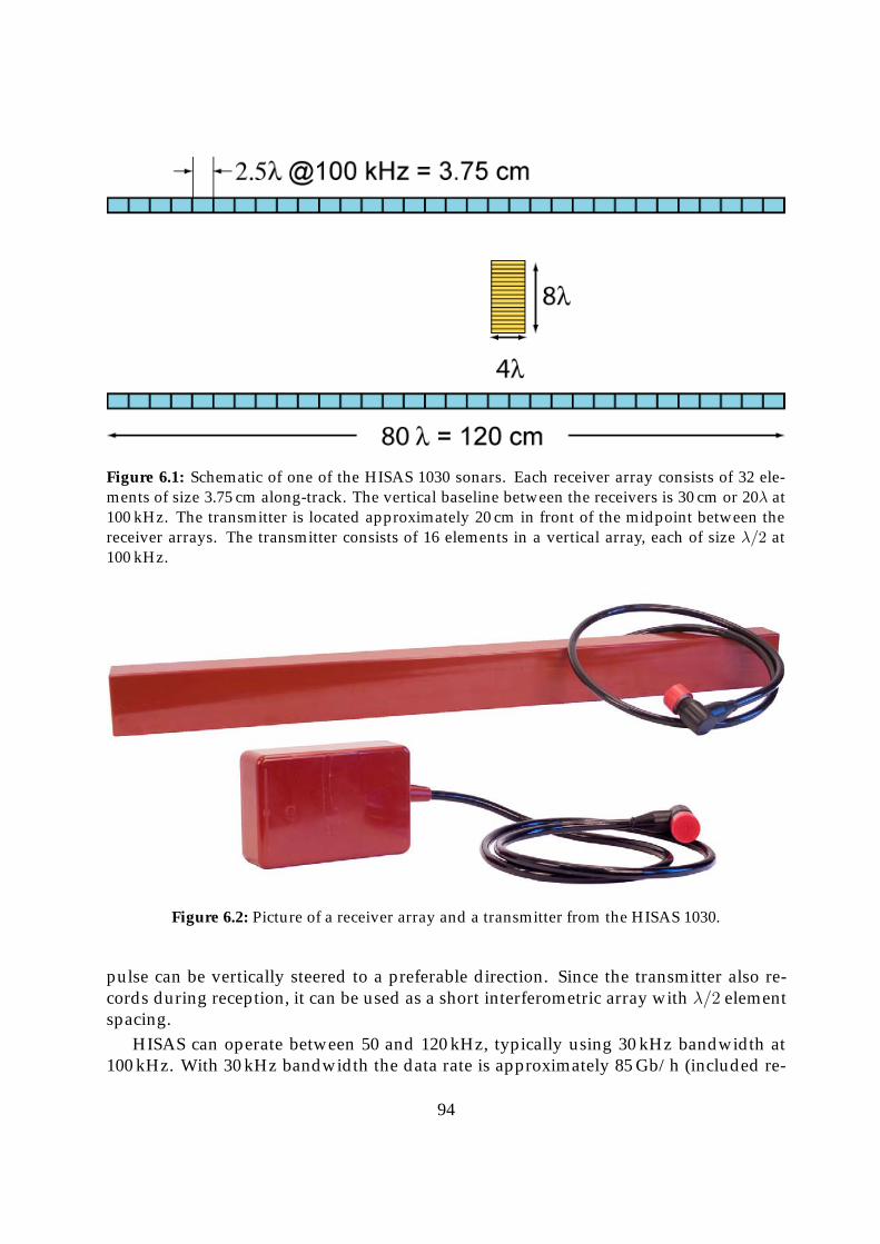
Figure 6.1: Schematic of one of the HISAS 1030 sonars. Each receiver array consists of 32 ele-ments of size 3.75 cm along-track. The vertical baseline between the receivers is 30 cm or 20λ at100 kHz. The transmitter is located approximately 20 cm in front of the midpoint between thereceiver arrays. The transmitter consists of 16 elements in a vertical array, each of size λ/2 at100 kHz.

Figure 6.2: Picture of a receiver array and a transmitter from the HISAS 1030.

pulse can be vertically steered to a preferable direction. Since the transmitter also re-cords during reception, it can be used as a short interferometric array with λ/2 elementspacing.

HISAS can operate between 50 and 120 kHz, typically using 30 kHz bandwidth at100 kHz. With 30 kHz bandwidth the data rate is approximately 85 Gb/h (included re-

94

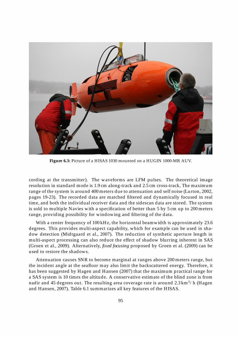
Figure 6.3: Picture of a HISAS 1030 mounted on a HUGIN 1000-MR AUV.

cording at the transmitter). The waveforms are LFM pulses. The theoretical imageresolution in standard mode is 1.9 cm along-track and 2.5 cm cross-track, The maximumrange of the system is around 400 meters due to attenuation and self noise (Lurton, 2002,pages 19-23). The recorded data are matched filtered and dynamically focused in realtime, and both the individual receiver data and the sidescan data are stored. The systemis sold to multiple Navies with a specification of better than 5 by 5 cm up to 200 metersrange, providing possibility for windowing and filtering of the data.

With a center frequency of 100 kHz, the horizontal beamwidth is approximately 23.6degrees. This provides multi-aspect capability, which for example can be used in sha-dow detection (Midtgaard et al., 2007). The reduction of synthetic aperture length inmulti-aspect processing can also reduce the effect of shadow blurring inherent in SAS(Groen et al., 2009). Alternatively, fixed focusing proposed by Groen et al. (2009) can beused to restore the shadows.

Attenuation causes SNR to become marginal at ranges above 200 meters range, butthe incident angle at the seafloor may also limit the backscattered energy. Therefore, ithas been suggested by Hagen and Hansen (2007) that the maximum practical range fora SAS system is 10 times the altitude. A conservative estimate of the blind zone is fromnadir and 45 degrees out. The resulting area coverage rate is around 2.3 km3/h (Hagenand Hansen, 2007). Table 6.1 summarizes all key features of the HISAS.

95

Table 6.1: Key features for the HISAS 1030 interferometric synthetic aperture sonar

Quantity Value

Receiver length 120 cm

Number of receive elements on each side 2x32

Vertical baseline 30 cm

Transmitter size 7.5x15 cm

Number of transmitter elements 8x16

Typical mounting roll angle 20 degrees

Frequencies 50-120 kHz

Typical operational bandwidth 30 kHz

Typical pulse type LFM

Typical pulse length 6 ms

Typical operational range 200 m

Theoretical resolution 1.9x2.5 cm

Practical resolution 5x5 cm

Theoretical area coverage rate 3.25 km2/h

Practical area coverage rate 2.3 km2/h

6.2 The HUGIN 1000-MR AUV

The HUGIN autonomous underwater vehicles have been developed by the Norwe-gian Defence Research Establishment (FFI) and Kongsberg Maritime (Hagen et al., 1999,2004, 2005). The development started in 1991 with a technology demonstrator, and thefirst sea trial took place in 1996. Originally, the HUGIN was designed for surveying indeep waters. With the HUGIN 1000-MR, the aim has been to develop an AUV especiallysuited for military purposes.

The HUGIN 1000-MR is modular in size (see Figure 6.4). The vehicle frame is madeof carbon fiber laminate and high performance syntactic foam. During operation, thevehicle is filled with water so the electronics is sheltered inside two spherical containers.Heavy equipment such as batteries and transducers can be used due to the buoyantframe. Typical dry weight of the vehicle is 600-800 kg.

The energy is delivered from two rechargeable Lithium polymer battery modulesand a high efficiency, high torque synchronous motor allows direct drive of a long bla-ded propeller. Four individually controlled rudder blades are used for heading, pitchand roll control. The vehicle is controlled by a distributed software system featuringthree or more main computers. The navigation processor runs the real-time integrated

96

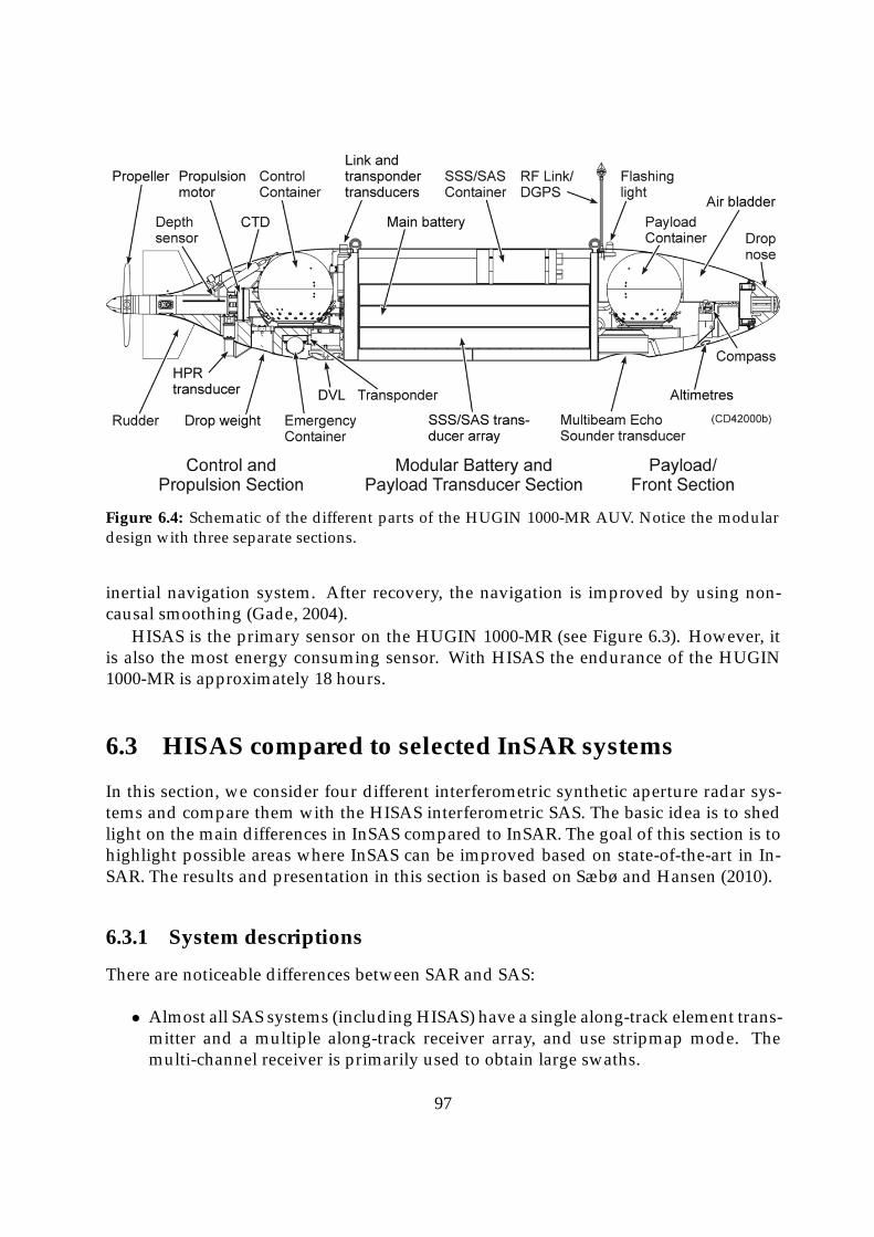
Figure 6.4: Schematic of the different parts of the HUGIN 1000-MR AUV. Notice the modulardesign with three separate sections.

inertial navigation system. After recovery, the navigation is improved by using non-causal smoothing (Gade, 2004).

HISAS is the primary sensor on the HUGIN 1000-MR (see Figure 6.3). However, itis also the most energy consuming sensor. With HISAS the endurance of the HUGIN1000-MR is approximately 18 hours.

6.3 HISAS compared to selected InSAR systems

In this section, we consider four different interferometric synthetic aperture radar sys-tems and compare them with the HISAS interferometric SAS. The basic idea is to shedlight on the main differences in InSAS compared to InSAR. The goal of this section is tohighlight possible areas where InSAS can be improved based on state-of-the-art in In-SAR. The results and presentation in this section is based on Sæbø and Hansen (2010).

6.3.1 System descriptions

There are noticeable differences between SAR and SAS:

• Almost all SAS systems (including HISAS) have a single along-track element trans-mitter and a multiple along-track receiver array, and use stripmap mode. Themulti-channel receiver is primarily used to obtain large swaths.

97

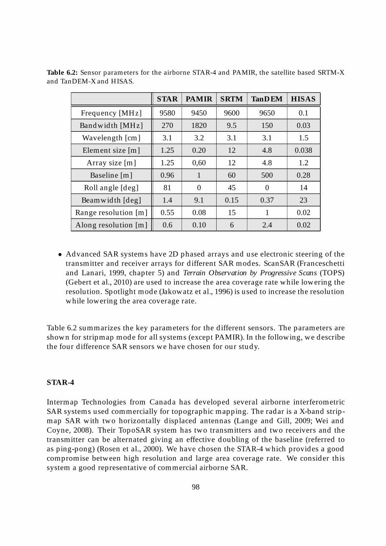
Table 6.2: Sensor parameters for the airborne STAR-4 and PAMIR, the satellite based SRTM-Xand TanDEM-X and HISAS.

STAR PAMIR SRTM TanDEM HISAS

Frequency [MHz] 9580 9450 9600 9650 0.1

Bandwidth [MHz] 270 1820 9.5 150 0.03

Wavelength [cm] 3.1 3.2 3.1 3.1 1.5

Element size [m] 1.25 0.20 12 4.8 0.038

Array size [m] 1.25 0,60 12 4.8 1.2

Baseline [m] 0.96 1 60 500 0.28

Roll angle [deg] 81 0 45 0 14

Beamwidth [deg] 1.4 9.1 0.15 0.37 23

Range resolution [m] 0.55 0.08 15 1 0.02

Along resolution [m] 0.6 0.10 6 2.4 0.02

• Advanced SAR systems have 2D phased arrays and use electronic steering of thetransmitter and receiver arrays for different SAR modes. ScanSAR (Franceschettiand Lanari, 1999, chapter 5) and Terrain Observation by Progressive Scans (TOPS)(Gebert et al., 2010) are used to increase the area coverage rate while lowering theresolution. Spotlight mode (Jakowatz et al., 1996) is used to increase the resolutionwhile lowering the area coverage rate.

Table 6.2 summarizes the key parameters for the different sensors. The parameters areshown for stripmap mode for all systems (except PAMIR). In the following, we describethe four difference SAR sensors we have chosen for our study.

STAR-4

Intermap Technologies from Canada has developed several airborne interferometricSAR systems used commercially for topographic mapping. The radar is a X-band strip-map SAR with two horizontally displaced antennas (Lange and Gill, 2009; Wei andCoyne, 2008). Their TopoSAR system has two transmitters and two receivers and thetransmitter can be alternated giving an effective doubling of the baseline (referred toas ping-pong) (Rosen et al., 2000). We have chosen the STAR-4 which provides a goodcompromise between high resolution and large area coverage rate. We consider thissystem a good representative of commercial airborne SAR.

98

PAMIR

The Phased Array Multifunctional Imaging Radar (PAMIR) is a high resolution phased ar-ray airborne SAR system with possibilities for cross-track interferometric mapping andalong-track interferometry moving target indication (MTI) (Ender and Brenner, 2003;Brenner and Roessing, 2008). The interferometric array includes three vertically spacedantennas with baselines of 0.67 meters and 0.335 meters, giving a total baseline of onemeter (Brenner and Roessing, 2008). This is a state-of-the-art airborne SAR, and witha recent upgrade to 3 GHz bandwidth the system has demonstrated SAR imagery witha resolution of 2 × 5 cm (Brenner, 2010). In repeat pass interferometry using a baselineof 17 m, PAMIR also demonstrated extreme resolution and accuracy in interferometry(Brenner et al., 2010). This radar is fully programmable and configurable. It is difficultto retrieve the actual performance from literature and we have therefore chosen para-meters from a sliding spotlight interferometry test (Brenner and Roessing, 2008). Thus,the actual parameters for stripmap interferometry might be incorrect. The system is stillinteresting to consider, representing state-of-the-art in airborne SAR.

SRTM-X

In 2000, the Shuttle Radar Topography Mission (SRTM) successfully recorded single passSAR interferometry data from the entire land mass of the earth between 60◦ N and 57◦

S, both in C-band and X-band (Rabus et al., 2003; Suchandt et al., 2006). This was thefirst single pass SAR interferometer in space. The maximum swath width of the C-bandsystem was 225 km in scansar mode using 4 beams, and 45 km in X-band stripmap mode(Rabus et al., 2003). The main antenna in the shuttle was 12 × 0.5meters large, and theoutboard antenna was 6 × 0.4meters for the X-band frequency. The secondary antennawas mounted on a 60 meters long boom to obtain a long baseline.

TanDEM-X

TerraSAR-X is a high resolution spaceborne SAR system for earth observations (Stanglet al., 2006). The radar antenna is a phased array with 384 elements, with the possibi-lity of multiple modes of operation: Stripmap mode with 3 meter resolution and 30 kmswath width; scansar mode with 16 meters resolution and 100 km swath width; andhigh resolution spotlight mode with one meter resolution and 10 km image size. InJune 2010 the TanDEM-X was launched (Krieger et al., 2007). This is an ad-on satelliteto TerraSAR-X for digital elevation mapping (DEM). Both satellites are considered onebistatic system with synchronous formation flying (Krieger et al., 2010) providing singlepass high resolution interferometry with large baselines. Both satellites will fly in helixtracks, forming both horizontal and vertical baselines up to several kilometers (Kriegeret al., 2010). The interferometric data collection with the two satellites can be perfor-med in different ways since both platforms have the possibility to transmit and receive.TanDEM-X represents state-of-the-art in horizontal resolution and vertical accuracy in

99

Table 6.3: Imaging geometry for the airborne STAR-4 and PAMIR, the satellite-borne SRTM-X and TanDEM-X, and HISAS. The parameters are shown for stripmap mode for all systems(except PAMIR).

STAR PAMIR SRTM TanDEM HISAS

Altitude [km] 8.5 3 233 515 0.02

Rmax [km] 17 7 410 728 0.2

Rsw,gr [km] 11 2 45 30 0.17

Rsw,sr [km] 7.7 1.7 36 21 0.17

Speed [m/s] 111 100 7500 7600 2

PRFmin [Hz] 178 333 1250 3167 3.33

PRFmax [Hz] 19430 86207 4167 7143 4.37

PRF [Hz] 1875 1000 1674 4500 3.75

SA length [m] 425 1111 1068 4740 80

SA time [s] 3.8 11 0.14 0.62 40

Nλ in SA 13600 35000 34167 151667 5333

Np in SA 7180 11000 238 2800 150

Rate [Mpixels/s] 2.2 25 3.75 95 0.85

spaceborne single pass interferometry.

6.3.2 Synthetic aperture data collection

There are fundamental differences between InSAR and InSAS in environmental condi-tions, phase velocity, geometry, data collection, platform motion and navigation (seeSection 2.5). In this section, we list some of the differences that affect synthetic aper-ture imaging and interferometry. Table 6.3 shows the key numbers for geometry anddata collection for the different sensors. The last row shows the data-rate defined asthe area coverage rate in square meters per second divided by the theoretical resolutionin square meters. This gives a indication of the hardware complexity and the requiredprocessing power.

The imaging geometry of existing SAS systems are very similar, with a swath rea-ching from nadir to roughly ten times the altitude. This geometry is very different fromspaceborne SAR systems, which have a much more vertical geometry. This reducesthe effect of shadowing, but increases the effect of foreshortening and layover (Frances-chetti and Lanari, 1999, page 37-41). An airborne SAR system usually has an imaginggeometry somewhere between a SAS and an spaceborne SAR. Figure 6.5 shows themeasurement geometry for the different sensors.

100

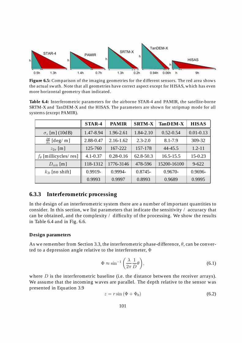
h

h 9h

h

0.94h 0.06h

h

1.4h 0.7h

HISAS

TanDEM-X

PAMIRh

0.5h 1.3h

STAR-4h

1.3h 0.2h

SRTM-X

Figure 6.5: Comparison of the imaging geometries for the different sensors. The red area showsthe actual swath. Note that all geometries have correct aspect except for HISAS, which has evenmore horizontal geometry than indicated.

Table 6.4: Interferometric parameters for the airborne STAR-4 and PAMIR, the satellite-borneSRTM-X and TanDEM-X and the HISAS. The parameters are shown for stripmap mode for allsystems (except PAMIR).

STAR-4 PAMIR SRTM-X TanDEM-X HISAS

σz [m] (10dB) 1.47-8.94 1.96-2.61 1.84-2.10 0.52-0.54 0.01-0.13∂θ∂z

[deg/m] 2.88-0.47 2.16-1.62 2.3-2.0 8.1-7.9 309-32

z2π [m] 125-760 167-222 157-178 44-45.5 1.2-11

fθ [millicycles/res] 4.1-0.37 0.28-0.16 62.8-50.3 16.5-15.5 15-0.23

Dcrit [m] 118-1312 1776-3146 478-596 15200-16100 9-622

kB [no shift] 0.9919- 0.9994- 0.8745- 0.9670- 0.9696-

0.9993 0.9997 0.8993 0.9689 0.9995

6.3.3 Interferometric processing

In the design of an interferometric system there are a number of important quantities toconsider. In this section, we list parameters that indicate the sensitivity / accuracy thatcan be obtained, and the complexity / difficulty of the processing. We show the resultsin Table 6.4 and in Fig. 6.6.

Design parameters

As we remember from Section 3.3, the interferometric phase-difference, θ, can be conver-ted to a depression angle relative to the interferometer, Φ

Φ ≈ sin−1

(λ

2π

1

Dθ

), (6.1)

where D is the interferometric baseline (i.e. the distance between the receiver arrays).We assume that the incoming waves are parallel. The depth relative to the sensor waspresented in Equation 3.9

z = r sin (Φ + Φ0) (6.2)

101

where r is the slant-range and Φ0 the roll of the interferometric array.A simple differentiation of Eqs. 6.1 and 6.2 gives the standard deviation of the depth

estimate as a function of the standard deviation of the phase-difference estimates σθ

σz =λ

2π

r

D

cos (Φ + Φ0)

cosΦσθ, (6.3)

where r, B and Φ0 are assumed known. Clearly, a large interferometric baseline withshort wavelengths gives the best performance (lowest standard deviation in depth).However, as we will see later, an increase in the interferometric baseline also causes areduction in coherence and robustness.

An important quantity is the height sensitivity (Bamler and Hartl, 1998)

∂θ

∂z=

2π

λ

D

r

cosΦ

cos (Φ + Φ0), (6.4)

which gives the phase-difference for a given geometry. Equivalently, this can be repre-sented by the height ambiguity, or the height which causes one phase wrap at a givenrange

z2π = 2π

(∂θ

∂z

)−1

= λr

D

cos (Φ + Φ0)

cos Φ. (6.5)

The local fringe frequency in range is a key parameter of the interferometer

fθ =1

2π

∂θ

∂r= −z

λ

D

r2cos Φ

cos (Φ + Φ0). (6.6)

This expression gives the change in phase-difference as a function of range and is identi-cal to the spectral shift of the signal. It can be used to calculate the maximum theoreticalcoherence between the receiver arrays. The critical baseline, Dcrit is the baseline whichgives a spectral shift equal to the bandwidth, B

Dcrit = λB

c

r2

z

cos (Φ + Φ0)

cosΦ. (6.7)

The baseline dependent coherence, kB, can be approximated as (Bamler and Hartl, 1998)

kD ≈ 1− D

Dcrit

forD Dcrit, (6.8)

with the total coherence written as

k = kSNRkDkT . (6.9)

Here kSNR is the coherence due to a finite SNR and kT is the temporal coherence.In Table 6.4 and Fig. 6.6 we summarize the most important interferometric features

for our example systems. There are rather large differences between the systems. Someof these are:

102

• HISAS has a large relative variation in range causing large variations in all thesensitivity parameters.

• TanDEM-X has large swath, high horizontal resolution and good vertical accuracydue to the large baseline.

• SRTM-X has relatively large spectral shift compared to the bandwidth.

• PAMIR has very low fringe frequency indicating that unwrapping is less difficult.

• STAR-4 has very large height ambiguity which indicates that unwrapping is notneeded.

• PAMIR, HISAS and STAR-4 have large critical baselines compared to the actualbaseline. This reduces the need to perform spectral shift filtering.

• TanDEM-X has a very large critical baseline, allowing for a high interferometricrange resolution.

• HISAS has a very low height ambiguity at short range. This indicates the need forgood unwrapping algorithms.

• STAR-4, PAMIR and SRTM-X have similar standard deviations of the height es-timate for fixed number of pixels and SNR. This means that PAMIR has muchhigher vertical accuracy for fixed horizontal patch in square meters, due to themuch higher resolution.

6.3.4 Summary

In this section, we have compared state-of-the-art interferometric SAR systems withthe HISAS sonar. We have chosen the systems somewhat subjectively in order to shedlight on what can be learned from InSAR. There are rather large differences between thedifferent SAR systems. The differences can be grouped in different ways. Spacebornesensors are different from airborne sensors. SAS is closer to airborne SAR. Complexand new sensors have better overall performance than simpler older sensors. This is inparticular apparent when comparing SRTM-X with TanDEM-X.

Interferometric SAS and HISAS in particular, has very large variations in the inter-ferometric performance over the entire swath due to the large range variation. At shortrange, the accuracy is extremely high, but the height ambiguity very low. At far range,the fringe frequency is very low and the critical baseline very high. At short range,phase unwrapping is probably the largest challenge, while at far range, lack of SNR isprobably the largest challenge. In sum, these findings suggests that optimal interfero-metric processing should be range dependent.

103

10−2

10−1

100

101

Normalized slant−rangeSta

ndar

d de

viat

ion

of h

eigh

t est

imat

e [m

]

STAR−4PAMIRSRTM−XTanDEM−XHISAS

100

101

102

103

Normalized slant−range

Hei

ght a

mbi

guity

[m]

STAR−4PAMIRSRTM−XTanDEM−XHISAS

10−4

10−3

10−2

10−1

Normalized slant−range

Frin

ge fr

eque

ncy

[cyc

les/

λ]

STAR−4PAMIRSRTM−XTanDEM−XHISAS

100

101

102

103

104

Normalized slant−range

Rel

ativ

e cr

itica

l bas

elin

e

STAR−4PAMIRSRTM−XTanDEM−XHISAS

Figure 6.6: Interferometric performance of the airborne STAR-4 and PAMIR, the spaceborneSRTM-X and TanDEM-X and HISAS as a function of normalized slant-range. Upper left: theore-tical height accuracy; Upper right: height ambiguity; Lower left: fringe frequency; Lower right:critical baseline.

HISAS has large relative bandwidth and large beamwidth compared to SAR sys-tems. This indicates that the split-bandwidth interferometry technique (see Section 8.3)can be considered to simplify or avoid unwrapping problems.

A trend in interferometric SAR is the use of repeat pass interferometry for deforma-tion mapping, temporal change detection and multi-baseline tomography. We believethat the future of InSAS brings these advanced techniques to the underwater environ-ment too (Synnes et al., 2010).

104

Chapter 7

Resolution and precision assessment

In this section we discuss the theoretical, the practical and the achievable resolutionand precision of the depth estimates. We focus on two quantities: Horizontal resolu-tion, i.e. the resolution in x, y or in along-track and cross-track projected down onto theseafloor (ground-range), and the precision in the depth estimate (precision along thez-coordinate). We will also separate between sidescan and SAS bathymetry, althoughmany of the arguments and equations will appear in both topics.

The horizontal resolutions of bathymetric estimates are complicated. We need to de-fine a sensible and applicable definition of resolution in a bathymetric map. We choosetwo different approaches: When calculating the resolutions mathematically, we start bythe underlying image resolution and investigate how the bathymetric processing mayaffect these measures. When we want to measure the achieved resolution in a bathyme-tric dataset we consider the flank of a distinct change in the bathymetry. We measurethe horizontal distance between where the bathymetry is at one level to where it hasreached the other level (assuming that the change in bathymetry is instantaneous andthat the change is significantly larger than the precision of the estimates, so that the twolevels can be easily separated). This estimate of resolution is ad-hoc and we do not claimthat it can be deduced from the theoretical measures, but it is strongly influenced by ourperception of resolution.

In this section and throughout the thesis, simulated data are generated using a pointscatter simulator (with a few exceptions in Chapter 4). The simulator uses independent,non-directive scatterers which are randomly distributed in the horizontal plane and arelocated on a virtual surface in the vertical plane. The strength of each scatterer is calcula-ted using a standard normal distribution. The simulator is implemented in time-domainand generates raw sonar data using LFM pulses. Sonar beampattern, transmission-lossand continuous motion through pings are simulated accurately. So is the sonar trajec-tory. However, the simulator does not simulate a realistic scene. The scattering mecha-nism is simplified and effects like shadow, multipath and specular reflections are omit-ted. A realistic speckle statistic is still achievable by choosing a large enough number ofscatterers in each resolution cell. In this thesis we use approximately ten reflectors (ormore) in each resolution cell. This means that a simulation for SAS interferometry has

105

to have a much higher density of scatterers than a simulation for sidescan bathymetry.

7.1 Sidescan bathymetry

As mentioned in Chapter 2, a sidescan image has a theoretical along-track resolution of(Van Trees, 2002, pages 46-51)

δssix ≈ λ

Lr =

λ

Nrdr, (7.1)

where λ is the wavelength, L = Nrd is the length of a receiver array consisting of Nr

elements of size d, and r is the range. Note that the along-track resolution is range-dependent and that this is the 3 dB resolution (i.e. a measure of the distance needed toseparate two targets of equal strength by 3 dB) (Van Trees, 2002, pages 46-51). Othertypes of resolution can be defined (Van Trees, 2002, pages 46-51). In Section 2 we alsodefined the theoretical 3 dB range resolution of a sidescan image as (Franceschetti andLanari, 1999, page 23)

δssir =c

2B, (7.2)

where c is the sound velocity and B the bandwidth of the system.In sidescan bathymetry we use a patch of data along a range-profile (i.e. a small seg-

ment of a time series) to estimate the depth (see Section 5.1.2). Therefore the theoreticalsidescan bathymetry resolution should equal the sidescan image resolution along-track,and the number of independent samples in the patch times the sidescan image resolu-tion cross-track. Along the array we do not apply any weighting, nor do we performany other kind of processing which will deteriorate the resolution so the practical (andtheoretical) along-track resolution in sidescan bathymetry equals the theoretical resolu-tion of the sidescan images

δssbx = δssix =λ

Nrdr. (7.3)

Cross track the story is more complicated. Firstly, we have to consider the lengthof the patch of data. Secondly, we apply a weighting after the matched filtering whichreduces the resolution. Thirdly, we render the sidescan image down onto a (non-flat)seafloor (which yields a resolution in y instead of in r). Fourthly, we apply weighting onthe patch data before we correlate the interferometric arrays (which effectively reducesthe size of the patch). The bathymetric y-resolution thus becomes

δssby = w1w2NsTryδssiy = w1w2NsTry

c

2B, (7.4)

where Ns is the number of independent samples in the patch, w1 a factor due to thewindow applied in the matched filter, w2 a factor due to the window applied on thepatch-data and Try a factor due to the resampling from range to y. While Ns can be

106

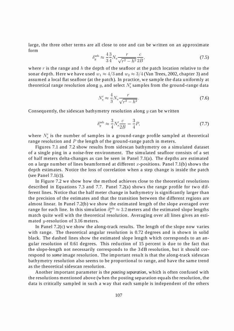
large, the three other terms are all close to one and can be written on an approximateform

δssby ≈ 4

3

3

4Ns

r√r2 − h2

c

2B, (7.5)

where r is the range and h the depth of the seafloor at the patch location relative to thesonar depth. Here we have used w1 ≈ 4/3 and w2 ≈ 3/4 (Van Trees, 2002, chapter 3) andassumed a local flat seafloor (at the patch). In practice, we sample the data uniformly attheoretical range resolution along y, and select N ′

s samples from the ground-range data

N ′s ≈

4

3Ns

r√r2 − h2

. (7.6)

Consequently, the sidescan bathymetry resolution along y can be written

δssby ≈ 3

4N ′

s

c

2B=

3

4P, (7.7)

where N ′s is the number of samples in a ground-range profile sampled at theoretical

range resolution and P the length of the ground-range patch in meters.Figures 7.1 and 7.2 show results from sidescan bathymetry on a simulated dataset

of a single ping in a noise-free environment. The simulated seafloor consists of a setof half meters delta-changes as can be seen in Panel 7.1(a). The depths are estimatedon a large number of lines beamformed at different x-positions. Panel 7.1(b) shows thedepth estimates. Notice the loss of correlation when a step change is inside the patch(see Panel 7.1(c)).

In Figure 7.2 we show how the method achieves close to the theoretical resolutionsdescribed in Equations 7.3 and 7.7. Panel 7.2(a) shows the range profile for two dif-ferent lines. Notice that the half meter change in bathymetry is significantly larger thanthe precision of the estimates and that the transition between the different regions arealmost linear. In Panel 7.2(b) we show the estimated length of the slope averaged overrange for each line. In this simulation δssby ≈ 3.2meters and the estimated slope lengthsmatch quite well with the theoretical resolution. Averaging over all lines gives an esti-mated y-resolution of 3.16 meters.

In Panel 7.2(c) we show the along-track results. The length of the slope now varieswith range. The theoretical angular resolution is 0.72 degrees and is shown in solidblack. The dashed lines show the estimated slope length which corresponds to an an-gular resolution of 0.61 degrees. This reduction of 15 percent is due to the fact thatthe slope-length not necessarily corresponds to the 3 dB resolution, but it should cor-respond to some image resolution. The important result is that the along-track sidescanbathymetry resolution also seems to be proportional to range, and have the same trendas the theoretical sidescan resolution.

Another important parameter is the posting separation, which is often confused withthe resolutions mentioned above (when the posting separation equals the resolution, thedata is critically sampled in such a way that each sample is independent of the others

107

X offset [m]

Gro

und−

rang

e [m

]

−4 −3 −2 −1 0 1 2 3 460

80

100

120

140

160

Dep

th [m

]

19.4

19.6

19.8

20

20.2

20.4

20.6

(a) Simulated seafloor

X offset [m]

Gro

und−

rang

e [m

]

−4 −3 −2 −1 0 1 2 3 460

80

100

120

140

160

Dep

th [m

]

19.4

19.6

19.8

20

20.2

20.4

20.6

(b) Estimated seafloor

60 80 100 120 140 1600.88

0.9

0.92

0.94

0.96

0.98

1

Ground−range [m]

Pea

k co

rrel

atio

n

(c) Averaged correlations

Figure 7.1: The figure shows results from sidescan bathymetry on a single simulated noise-freeping. The bathymetry is estimated on a number of offset beams. Panel (a) shows the simulatedseafloor, while the estimated seafloor is presented in panel (b). Panel (c) shows the peak correla-tions as a function of ground-range averaged over offset beams. The beams close to zero offsetare omitted, since they are affected by the along-track bathymetric change.

108

60 80 100 120 140 160

19.2

19.4

19.6

19.8

20

20.2

20.4

20.6

Ground−range [m]

Dep

th [m

]

x=−5 mx=5 m

(a) Estimated range profiles

−5 −4 −3 −2 −1 0 1 2 3 4 52.9

3

3.1

3.2

3.3

3.4

X offset [m]

Gro

und−

rang

e re

solu

tion

[m]

EstimatedAverageTheoretical

(b) Estimated resolution along ground-range

−2.5 −2 −1.5 −1 −0.5 0 0.5 1 1.5 2 2.5X offset [m]

Nor

mal

ised

dep

th e

stim

ates

Theoretical resolutionEstimated resolution

(c) Estimated resolution along-track

Figure 7.2: The figure shows results from sidescan bathymetry on a single simulated noise-free ping. The bathymetry is estimated on a number of offset beams. Panel (a) shows twoof the estimated range profiles, offset 5 meters from broadside. Panel (b) shows the estima-ted ground-range resolution for each offset line. Panel (c) shows cross-sections along-track atdifferent ranges. The colored lines represent different ranges. The theoretical and estimated re-solutions are drawn on top. Notice that the apparent asymmetrical beam pattern is caused bythe fact that the range changes with the bathymetry when the ground-range is kept constant.

109

0 20 40 60 80 100 120 140 160 180 2000

5

10

15

20

Ground−range [m]

ST

D o

f dep

th e

stim

ate

[cm

]

0dB10dB20dB30dB

Figure 7.3: STD of the sidescan bathymetry depth estimate errors as a function of ground-rangefor a set of different SNRs. The results are calculated from Equation 7.8 with D=0.28 meters,f0=100 kHz, c=1500 m/s and N = 128 cos (Φ), with Φ = tan−1 (h/rg) where gr is the ground-range and h = 20 is the depth of the seafloor relative to the sonar.

and no information is lost due to undersampling). In sidescan bathymetry, the postingseparation along x is given by the motion of the sensor between pings. Since the sensorcan change its pointing direction from one ping to another, the posting separation maychange as a function of ping and range (it may even become zero). For a SAS-systemit usually equals slightly less than half the array-length. For HISAS it is typically 0.5meter. Along ground-range y, the posting separation can be chosen arbitrarily, onlyaffecting processing time. We use one meter as default. This gives an oversamplingwhich ensures that the estimated surface is sufficiently continuous and smooth.

Next we consider the accuracy and precision of sidescan bathymetry. We defineprecision as a measure of the error relative to the true answer. In the case where thereare no ambiguities and no bias, the precision equals the accuracy, which is a measureof noise in the estimates. In this thesis we mostly assume bias- and ambiguity-freeestimates in the mathematical calculations, which means that we only calculates theaccuracy. The precision is discussed by comparing results with the ground truth, whereavailable, or by observing obvious flaws in the estimates.

As mentioned in Section 4.5 there are two different expressions which describe theaccuracy of interferometric time delay estimation. Either one uses Equation 4.39 andassumes that the recorded data are deterministic, time delayed time series (which theyare not, since the signal is scattered from a 3D geometry), or one uses Equation 4.40 andassumes that the recorded data are co-registered datasets with speckle statistics (whichbreaks down when there are objects on the seafloor). Since the two expressions areclose to but not equal, we have chosen to consider sidescan bathymetry as time delayestimation and SAS interferometry as interferometric processing.

Combining Equations 3.24 and 4.39 gives an expression for the standard deviation

110

of the sidescan bathymetry estimates

std{zest} ≈ cr22D

1

2πf0

1√N

√1

ρ+

1

2ρ2, (7.8)

where c is the sound speed, r2 the range from receiver #2 to the seafloor, D the verticalbaseline,N the number of independent samples and f0 the center frequency. Rememberfrom Equation 4.17 that the SNR, ρ, can be estimated from the coherence.

Figure 7.3 shows results from Equation 7.8 using HISAS settings, i.e. D=0.28 metersand f0=100 kHz. The sound speed, c, is set to 1500 m/s and we have used a fixed patchlength of 3.2 meters in ground-range. This is equivalent to N = 128 cos (Φ) independentsamples, where Φ is the depression angle. The increase at short range in Figure 7.3 iscaused by the increasing depression angle, which reduces the number of independentsamples in the patch. From the figure we see that a 10 dB SNR is sufficient to achieve aSTD of the depth-error always less than 5 cm. This is around the desired performance,the problem is to achieve >10 dB at 200 meters range.

To evaluate if the theoretical accuracy is met, we have simulated a flat seafloor with120000 reflectors scattered randomly out to 200 meters range. AWGN is added to thereceived time series and the estimated depths averaged over 1000 pings. The results canbe found in Figure 7.4. The two upper panels show the coherence and correspondingSNR from the estimates. They also show the results from measuring the SNR directly onthe simulated raw-data. A comparison reveals three distinct features: At short range theSNR from the peak correlation coefficient meets a threshold and falls of. This is causedby a combination of interpolation inaccuracies and baseline decorrelation. At mediumrange the two SNR estimates correspond quite well. At far range the SNR from the peakcorrelation coefficient falls of again. This discrepancy is yet to be explained.

The third panel in Figure 7.4 shows the STD and RMS error of the sidescan bathyme-try depth estimates. These two quantities are almost identical, indicating that there isno significant bias in the estimates. In the same panel the predicted performance fromthe SNR estimates are included. They show a good correspondence with the estimatederror. However, one can notice that the fall in peak correlation at far range increases thepredicted STD, but it does not affect the actual performance of the depth estimates. Thissuggests that the peak correlation coefficient is unreliable when it falls below around 0.7(which fits well with our correlation threshold value of 0.66).

The lower panel of Figure 7.4 summaries the sidescan bathymetry performance. Itshows that the ratio between the achieved STD of the depth-error and the predictedSTD from the peak correlation coefficient is close to one. This means that Equation 7.8can give a good estimate of the performance of sidescan bathymetry, when the SNR iscalculated from the peak correlation coefficient. It also show that there is a significantloss in performance at short range mostly caused by geometrical effects. But since theperformance is proportional to range, this effect is less significant for the overall perfor-mance.

The results from a large scale simulation of the sidescan bathymetry performancecan be found in Figure 7.5. Part of a real AUV trajectory is used in the simulation, which

111

0.2

0.4

0.6

0.8

1

Coh

eren

ce

From correlationFrom time series

0

10

20

30

40

SN

R [d

B]

From correlationFrom time series

0

0.05

0.1

0.15

0.2

Dep

th−

erro

r [m

]

STDRMSEFrom correlationFrom time series

40 60 80 100 120 140 160 180 2000

5

10

15

20

25

Ground−range [m]

Exc

ess

erro

r fa

ctor

From correlationFrom time series

Figure 7.4: Results from averaging 1000 pings of sidescan bathymetry depth estimates on a flatsimulated seafloor with AWGN. A HISAS sonar is used in the simulation. The upper panelshows coherence as a function of ground-range. The solid line shows the peak correlation coef-ficient from sidescan bathymetry while the dashed line show the coherence calculated from theinserted SNR. The second panel shows the corresponding SNR as a function of ground-range.The third panel shows the STD (solid line) and RMS error (dotted line) of the sidescan bathy-metry depth estimates as a function of ground-range. We also show the predicted STD from thepeak correlation coefficient (dashed line) and from the inserted SNR (dashed-dotted line). Thelower panel shows the ratio between the estimated STD and the predicted STD (from the peakcorrelation coefficient) (solid line) as a function of ground-range. The dashed line shows theratio between the estimated STD and the predicted STD (from the inserted SNR).

112

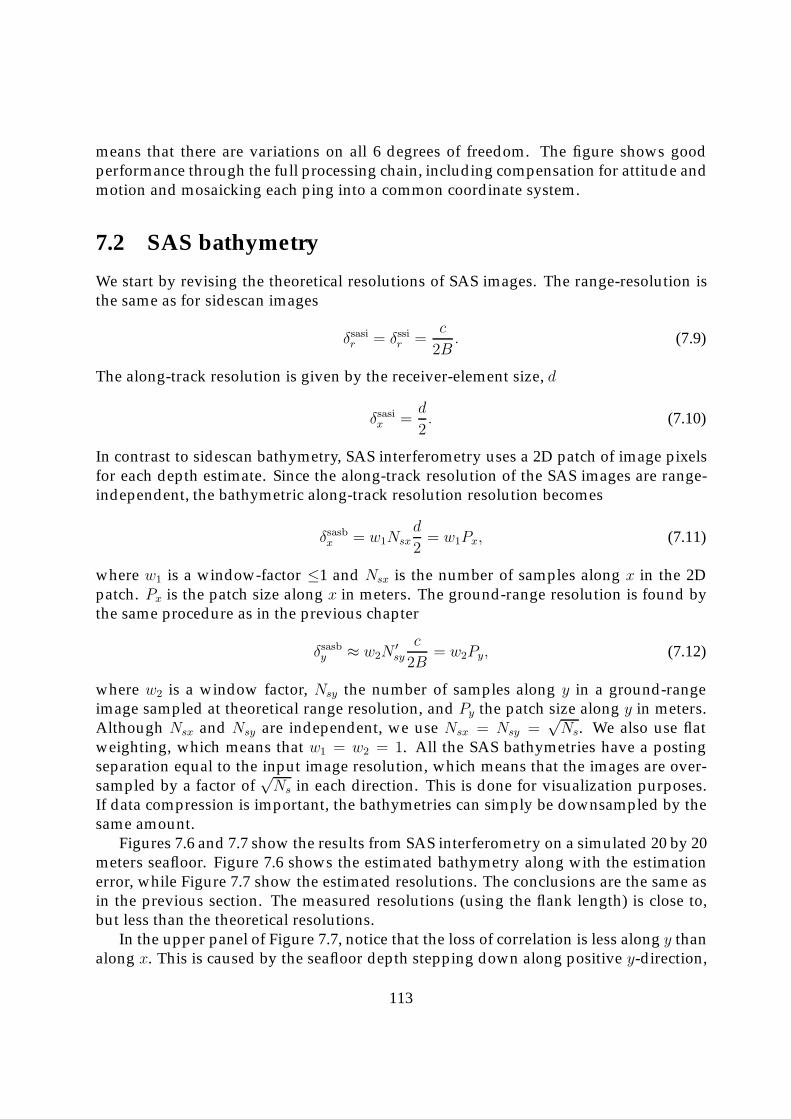
means that there are variations on all 6 degrees of freedom. The figure shows goodperformance through the full processing chain, including compensation for attitude andmotion and mosaicking each ping into a common coordinate system.

7.2 SAS bathymetry

We start by revising the theoretical resolutions of SAS images. The range-resolution isthe same as for sidescan images

δsasir = δssir =c

2B. (7.9)

The along-track resolution is given by the receiver-element size, d

δsasix =d

2. (7.10)

In contrast to sidescan bathymetry, SAS interferometry uses a 2D patch of image pixelsfor each depth estimate. Since the along-track resolution of the SAS images are range-independent, the bathymetric along-track resolution resolution becomes

δsasbx = w1Nsxd

2= w1Px, (7.11)

where w1 is a window-factor ≤1 and Nsx is the number of samples along x in the 2Dpatch. Px is the patch size along x in meters. The ground-range resolution is found bythe same procedure as in the previous chapter

δsasby ≈ w2N′sy

c

2B= w2Py, (7.12)

where w2 is a window factor, Nsy the number of samples along y in a ground-rangeimage sampled at theoretical range resolution, and Py the patch size along y in meters.Although Nsx and Nsy are independent, we use Nsx = Nsy =

√Ns. We also use flat

weighting, which means that w1 = w2 = 1. All the SAS bathymetries have a postingseparation equal to the input image resolution, which means that the images are over-sampled by a factor of

√Ns in each direction. This is done for visualization purposes.

If data compression is important, the bathymetries can simply be downsampled by thesame amount.

Figures 7.6 and 7.7 show the results from SAS interferometry on a simulated 20 by 20meters seafloor. Figure 7.6 shows the estimated bathymetry along with the estimationerror, while Figure 7.7 show the estimated resolutions. The conclusions are the same asin the previous section. The measured resolutions (using the flank length) is close to,but less than the theoretical resolutions.

In the upper panel of Figure 7.7, notice that the loss of correlation is less along y thanalong x. This is caused by the seafloor depth stepping down along positive y-direction,

113

Northings [m]

Eas

tings

[m]

0 50 100 150 200 250 300 350 400 450

0

50

100 Sim

ulat

ed d

epth

[m]

66

68

70

72

74

76

78

Northings [m]

Eas

tings

[m]

0 50 100 150 200 250 300 350 400 450

0

50

100 Est

imat

ed d

epth

[m]

66

68

70

72

74

76

78

Northings [m]

Eas

tings

[m]

0 50 100 150 200 250 300 350 400 450

0

50

100D

epth

est

imat

ion

erro

r [c

m]

−30

−20

−10

0

10

20

30

Figure 7.5: The upper panel shows a simulated bathymetry for a point scatter simulation with120000 reflectors. The simulated trajectory showed in solid black consists of 1000 pings from atrue AUV trajectory. The center panel shows the estimated bathymetry using sidescan bathyme-try with 200 patches one meter separated. The results are mosaicked into a half-meter grid andareas with no coverage or with a correlation value below 0.66 is colored white. The lower panelshows error in the estimates. Notice that the error increases with range.

114

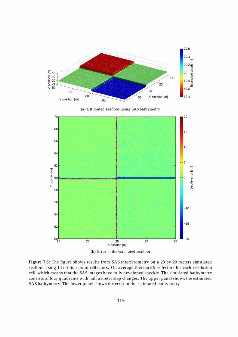
(a) Estimated seafloor using SAS bathymetry

X position [m]

Y p

ositi

on [m

]

15 20 25 30 3550

52

54

56

58

60

62

64

66

68

70

Dep

th−

erro

r [c

m]

−20

−15

−10

−5

0

5

10

15

20

(b) Error in the estimated seafloor

Figure 7.6: The figure shows results from SAS interferometry on a 20 by 20 meters simulatedseafloor using 13 million point reflectors. On average there are 9 reflectors for each resolutioncell, which means that the SAS images have fully developed speckle. The simulated bathymetryconsists of four quadrants with half a meter step changes. The upper panel shows the estimatedSAS bathymetry. The lower panel shows the error in the estimated bathymetry.

115

0 2 4 6 8 10 12 14 16 18 200.93

0.94

0.95

0.96

0.97

0.98

0.99

1

Normalised position [m]

Pea

k co

rrel

atio

n

Along xAlong y

(a) Averaged coherences

15 17 19 21 23 25 27 29 31 33 355

10

15

20

25

30

35

40

Y position [m]

Res

olut

ion

in x

[cm

]

EstimatedAverageTheoretical

(b) Estimated resolution along x

50 52 54 56 58 60 62 64 66 68 7010

15

20

25

30

35

40

45

X−position [m]

Res

olut

ion

in y

[cm

]

EstimatedAverageTheoretical

(c) Estimated resolution along y

Figure 7.7: The figure shows detailed results from the estimated bathymetry in Figure 7.6. Theupper panel shows the peak correlation coefficients averaged over each direction. The solid lineshows the correlation as a function of x-position averaged along y-positions, while the dashedline show the correlation as a function of y-position averaged along x-positions. The drop incorrelation is caused by the step change in the bathymetry. The center panel shows the estimatedx-resolutions using flank length. The lower panel shows the corresponding y-resolutions. Thetheoretical and average resolutions are drawn on top.

116

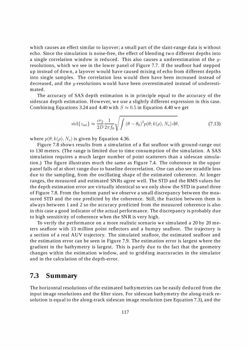
which causes an effect similar to layover; a small part of the slant-range data is withoutecho. Since the simulation is noise-free, the effect of blending two different depths intoa single correlation window is reduced. This also causes a underestimation of the y-resolutions, which we see in the lower panel of Figure 7.7. If the seafloor had steppedup instead of down, a layover would have caused mixing of echo from different depthsinto single samples. The correlation loss would then have been increased instead ofdecreased, and the y-resolutions would have been overestimated instead of underesti-mated.

The accuracy of SAS depth estimation is in principle equal to the accuracy of thesidescan depth estimation. However, we use a slightly different expression in this case.Combining Equations 3.24 and 4.40 with S ≈ 0.5 in Equation 4.40 we get

std{zest} ≈ cr22D

1

2πf0

√∫(θ − θ0)

2p(θ; k(ρ), Ns) dθ, (7.13)

where p(θ; k(ρ), Ns) is given by Equation 4.36.Figure 7.8 shows results from a simulation of a flat seafloor with ground-range out

to 130 meters. (The range is limited due to time consumption of the simulation. A SASsimulation requires a much larger number of point scatterers than a sidescan simula-tion.) The figure illustrates much the same as Figure 7.4. The coherence in the upperpanel falls of at short range due to baseline decorrelation. One can also see straddle lossdue to the sampling, from the oscillating shape of the estimated coherence. At longerranges, the measured and estimated SNRs agree well. The STD and the RMS values forthe depth estimation error are virtually identical so we only show the STD in panel threeof Figure 7.8. From the bottom panel we observe a small discrepancy between the mea-sured STD and the one predicted by the coherence. Still, the fraction between them isalways between 1 and 2 so the accuracy predicted from the measured coherence is alsoin this case a good indicator of the actual performance. The discrepancy is probably dueto high sensitivity of coherence when the SNR is very high.

To verify the performance on a more realistic scenario we simulated a 20 by 20 me-ters seafloor with 13 million point reflectors and a bumpy seafloor. The trajectory isa section of a real AUV trajectory. The simulated seafloor, the estimated seafloor andthe estimation error can be seen in Figure 7.9. The estimation error is largest where thegradient in the bathymetry is largest. This is partly due to the fact that the geometrychanges within the estimation window, and to gridding inaccuracies in the simulatorand in the calculation of the depth-error.

7.3 Summary

The horizontal resolutions of the estimated bathymetries can be easily deduced from theinput image resolutions and the filter sizes. For sidescan bathymetry the along-track re-solution is equal to the along-track sidescan image resolution (see Equation 7.3), and the

117

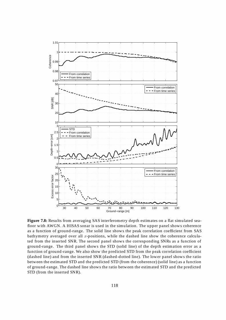
0.97

0.98

0.99

1

1.01

Coh

eren

ce

From correlationFrom time series

10

20

30

40

50

SN

R [d

B]

From correlationFrom time series

0

0.5

1

1.5

2

2.5

3

Dep

th−

erro

r [c

m]

STDFrom correlationFrom time series

30 40 50 60 70 80 90 100 110 120 1300

5

10

15

20

25

30

Ground−range [m]

Exc

ess

erro

r fa

ctor

From correlationFrom time series

Figure 7.8: Results from averaging SAS interferometry depth estimates on a flat simulated sea-floor with AWGN. A HISAS sonar is used in the simulation. The upper panel shows coherenceas a function of ground-range. The solid line shows the peak correlation coefficient from SASbathymetry averaged over all x-positions, while the dashed line show the coherence calcula-ted from the inserted SNR. The second panel shows the corresponding SNRs as a function ofground-range. The third panel shows the STD (solid line) of the depth estimation error as afunction of ground-range. We also show the predicted STD from the peak correlation coefficient(dashed line) and from the inserted SNR (dashed-dotted line). The lower panel shows the ratiobetween the estimated STD and the predicted STD (from the coherence) (solid line) as a functionof ground-range. The dashed line shows the ratio between the estimated STD and the predictedSTD (from the inserted SNR).

118

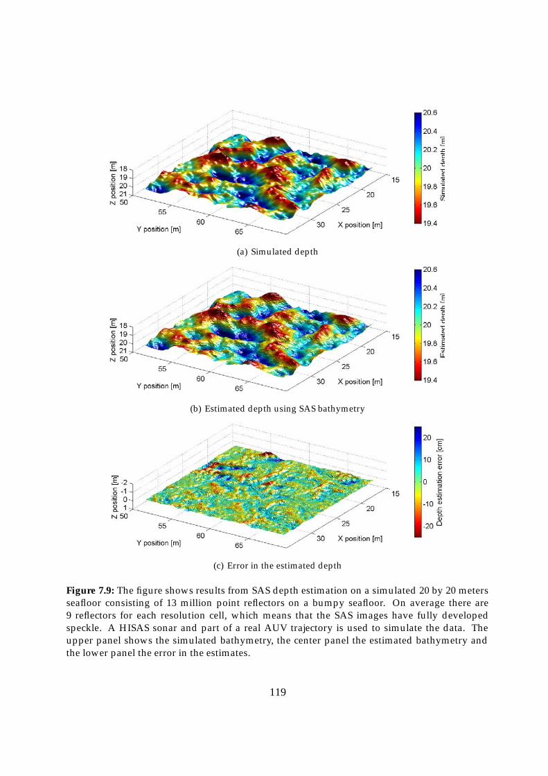
(a) Simulated depth

(b) Estimated depth using SAS bathymetry

(c) Error in the estimated depth

Figure 7.9: The figure shows results from SAS depth estimation on a simulated 20 by 20 metersseafloor consisting of 13 million point reflectors on a bumpy seafloor. On average there are9 reflectors for each resolution cell, which means that the SAS images have fully developedspeckle. A HISAS sonar and part of a real AUV trajectory is used to simulate the data. Theupper panel shows the simulated bathymetry, the center panel the estimated bathymetry andthe lower panel the error in the estimates.

119

cross-track resolution is equal to the effective ground-range patch-length (see Equation7.7). For SAS bathymetry, the resolutions are equal to the size of the estimation windowin both dimensions (see Equations 7.11 and 7.12). These findings are in agreement withsimulation results using flank length as a resolution measure.

The accuracies can be found either from time delay theory or from speckle statistics.For sidescan depth estimation we use time delay theory (see Equation 7.8) and find thatthe accuracy predicted from the measured peak correlation value corresponds well withthe measured accuracy on a simulated dataset. For SAS depth estimation we use specklestatistics and found that the predicted accuracy (see Equation 7.13) is in agreement withthe measured accuracy within a factor two, when the measured coherence is used in thepredictions (i.e. the measured accuracy is between the theoretical accuracy and twicethe theoretical accuracy).

120

Chapter 8

Results and studies

In this chapter we present analysis and results from selected studies. Some of the ma-terial is presented for the first time while other parts are reproductions from previouslypublished material.

8.1 The phase-difference filter size and shape

The vertical accuracy and the horizontal resolutions of SAS bathymetry are dependenton the number of independent image-pixels used to estimate each depth (see Chapter7). In this section we consider the effect of changing filter sizes in the phase-differenceestimator (see Equation 4.29). We also examine the effect of different weights applied inthe filter and of down-sampling the resulting depth maps. The results and presentationin this section is based on Sæbø et al. (2007c).

As we discussed in Chapter 7, both the vertical accuracy and the horizontal reso-lutions of SAS bathymetry are dependent on the number of independent image-pixelsused to estimate each depth. Our implementation of the phase-difference estimator issuch that the input gridding is not changed. For some applications, the most elevatedfeature in each resolution cell is more important than the average depth so any down-sampling must retain peaks if they exist in the bathymetry. A technique which keeps theshallowest depth values can then be applied to reduce the sample density to a suitablequantity for charting of large areas.

Depending on the application, different resolutions and different grid samplingsmay be desired. Resampling can be implemented in different ways at different levels inthe processing

• Pre-processing: For a critically sampled SAS image one can reduce the resolu-tion by either reducing the wavenumber coverage, or by incoherent averaging in-dependent wavenumber regions or by simply selecting only some of the pixels.The third option is clearly suboptimal since it will produce an undersampledimage. The second option can be used to reduce the amount of speckle (Jako-watz et al., 1996, pages 112-121), but incoherent averaging will destroy the phase

121

in the images. The first option is the best solution, but it should be noted thatwhen considering bathymetric accuracy, it is always better to have as high as pos-sible resolution in the input SAS images and rather perform down-sampling at alater stage. However, reducing wavenumber coverage reduces the computationtime of both SAS image formation and of interferometric processing and that mayoutweigh the disadvantages in some cases.

• Filtering: The maximum likelihood phase filter reduces the resolution to the sizeof the applied filtering window, but retains the input grid sampling (see Chapter7).

• Post-processing: At this step, the interferogram is oversampled with the size ofthe applied filter. Resampling the interferogram or the bathymetry is almost iden-tical, since the geometrical conversions from phase-differences to depths are closeto linear in small regions. Oversampled depth estimates give a smoother visuali-zation of the bathymetry and is often the best choice for smaller regions. For largerregions, we want to reduce the data-amount and down-sample the grid samplingto the actual resolution. In some cases, even further down-sampling may be desi-red. Again there are several options. For optimum visualization, a simple averagefilter can be applied. For bathymetric mapping, picking the highest point in eachcell may be a more robust solution. More advanced methods may use the SASreflectivity in the down-sampling.

Theoretically, SAS bathymetry can provide depth maps with image resolution. Thephase-difference can simply be estimated for each image pixel-pair without any filte-ring. Due to the speckly nature of the SAS images this works poorly in practice; theecho strength is random and, assuming a fixed noise level, will cause variations in theSNR. The precision of the depth estimates will therefore vary strongly, causing unaccep-table low robustness. To illustrate the effect of different filtering techniques on real data,we have selected data from a simulated bumpy seafloor with random distributed pointscatterers. Figure 8.1 shows the estimated bathymetry with and without the phase-filtering. Clearly, the depth maps agree to a large extent, but random pixels seem to failfor the full-resolution case. The simulation is noise-free and therefore also a best casescenario; introducing noise will only increase the problems for the full-resolution case.A noisy seafloor like the one in the lower panel of Figure 8.1 is not for post-processingor 3D-visualization.

To investigate the effect of different filtering techniques we selected an area outsideHorten, Norway at around 200 meters water depth. The scene consists of a relativelyflat seafloor with a 3 by 10 meters barge located in the middle. The imagery is generatedusing INS integrated DPCA motion estimates and wavenumber beamforming, and hasa final resolution of 2.94 cm by 1.37 cm (along-track by range). Figure 8.2 shows the SASimage, the estimated bathymetry and the coherence using a standard filtering size of9× 9 pixels. Note the lack of coherence in the shadow regions.

122

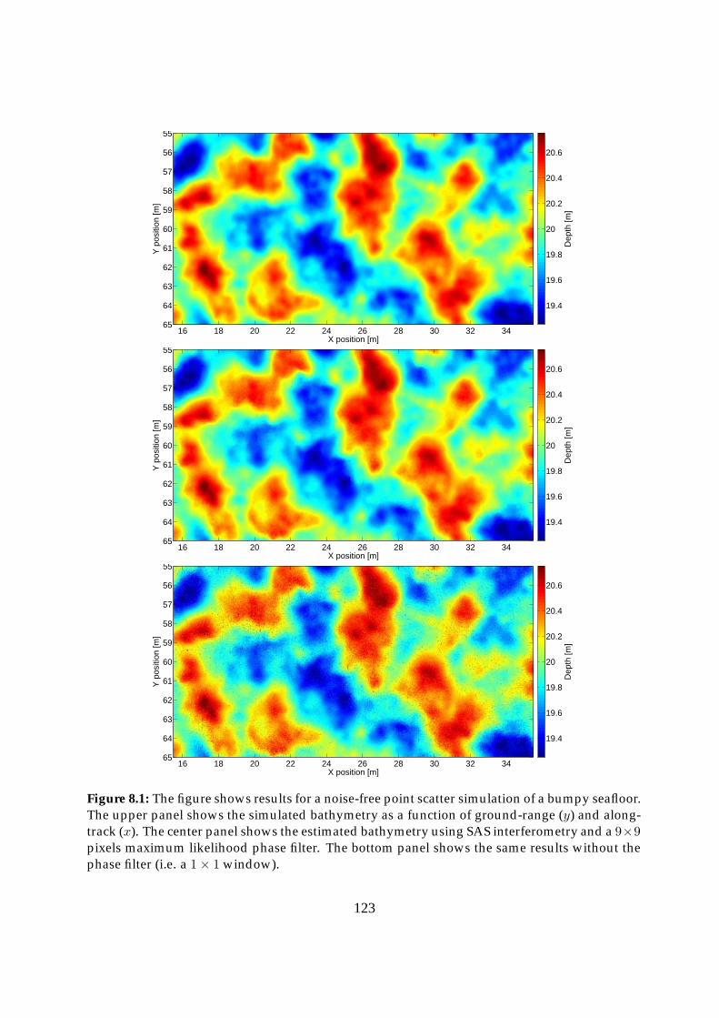
X position [m]

Y p

ositi

on [m

]

16 18 20 22 24 26 28 30 32 34

55

56

57

58

59

60

61

62

63

64

65

Dep

th [m

]

19.4

19.6

19.8

20

20.2

20.4

20.6

X position [m]

Y p

ositi

on [m

]

16 18 20 22 24 26 28 30 32 34

55

56

57

58

59

60

61

62

63

64

65

Dep

th [m

]

19.4

19.6

19.8

20

20.2

20.4

20.6

X position [m]

Y p

ositi

on [m

]

16 18 20 22 24 26 28 30 32 34

55

56

57

58

59

60

61

62

63

64

65

Dep

th [m

]

19.4

19.6

19.8

20

20.2

20.4

20.6

Figure 8.1: The figure shows results for a noise-free point scatter simulation of a bumpy seafloor.The upper panel shows the simulated bathymetry as a function of ground-range (y) and along-track (x). The center panel shows the estimated bathymetry using SAS interferometry and a 9×9pixels maximum likelihood phase filter. The bottom panel shows the same results without thephase filter (i.e. a 1× 1 window).

123

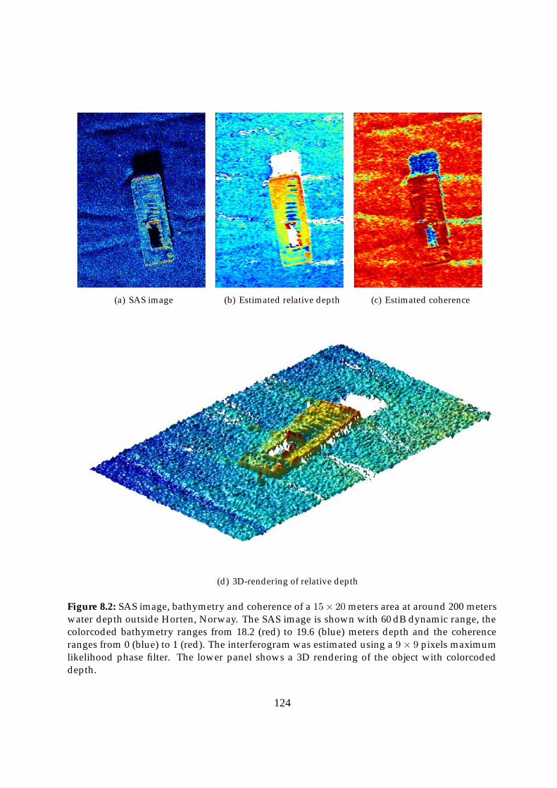
(a) SAS image (b) Estimated relative depth (c) Estimated coherence

(d) 3D-rendering of relative depth

Figure 8.2: SAS image, bathymetry and coherence of a 15× 20 meters area at around 200 meterswater depth outside Horten, Norway. The SAS image is shown with 60 dB dynamic range, thecolorcoded bathymetry ranges from 18.2 (red) to 19.6 (blue) meters depth and the coherenceranges from 0 (blue) to 1 (red). The interferogram was estimated using a 9× 9 pixels maximumlikelihood phase filter. The lower panel shows a 3D rendering of the object with colorcodeddepth.

124

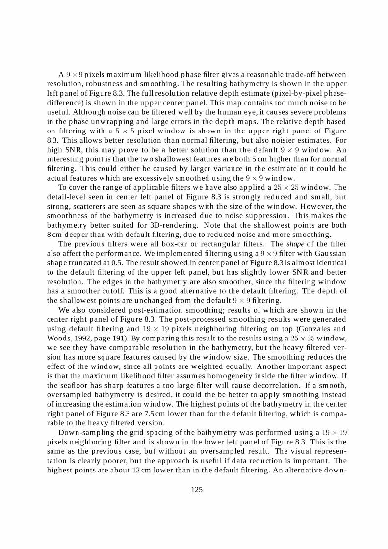
A 9× 9 pixels maximum likelihood phase filter gives a reasonable trade-off betweenresolution, robustness and smoothing. The resulting bathymetry is shown in the upperleft panel of Figure 8.3. The full resolution relative depth estimate (pixel-by-pixel phase-difference) is shown in the upper center panel. This map contains too much noise to beuseful. Although noise can be filtered well by the human eye, it causes severe problemsin the phase unwrapping and large errors in the depth maps. The relative depth basedon filtering with a 5 × 5 pixel window is shown in the upper right panel of Figure8.3. This allows better resolution than normal filtering, but also noisier estimates. Forhigh SNR, this may prove to be a better solution than the default 9 × 9 window. Aninteresting point is that the two shallowest features are both 5 cm higher than for normalfiltering. This could either be caused by larger variance in the estimate or it could beactual features which are excessively smoothed using the 9× 9 window.

To cover the range of applicable filters we have also applied a 25 × 25 window. Thedetail-level seen in center left panel of Figure 8.3 is strongly reduced and small, butstrong, scatterers are seen as square shapes with the size of the window. However, thesmoothness of the bathymetry is increased due to noise suppression. This makes thebathymetry better suited for 3D-rendering. Note that the shallowest points are both8 cm deeper than with default filtering, due to reduced noise and more smoothing.

The previous filters were all box-car or rectangular filters. The shape of the filteralso affect the performance. We implemented filtering using a 9× 9 filter with Gaussianshape truncated at 0.5. The result showed in center panel of Figure 8.3 is almost identicalto the default filtering of the upper left panel, but has slightly lower SNR and betterresolution. The edges in the bathymetry are also smoother, since the filtering windowhas a smoother cutoff. This is a good alternative to the default filtering. The depth ofthe shallowest points are unchanged from the default 9× 9 filtering.

We also considered post-estimation smoothing; results of which are shown in thecenter right panel of Figure 8.3. The post-processed smoothing results were generatedusing default filtering and 19 × 19 pixels neighboring filtering on top (Gonzales andWoods, 1992, page 191). By comparing this result to the results using a 25× 25 window,we see they have comparable resolution in the bathymetry, but the heavy filtered ver-sion has more square features caused by the window size. The smoothing reduces theeffect of the window, since all points are weighted equally. Another important aspectis that the maximum likelihood filter assumes homogeneity inside the filter window. Ifthe seafloor has sharp features a too large filter will cause decorrelation. If a smooth,oversampled bathymetry is desired, it could the be better to apply smoothing insteadof increasing the estimation window. The highest points of the bathymetry in the centerright panel of Figure 8.3 are 7.5 cm lower than for the default filtering, which is compa-rable to the heavy filtered version.

Down-sampling the grid spacing of the bathymetry was performed using a 19 × 19pixels neighboring filter and is shown in the lower left panel of Figure 8.3. This is thesame as the previous case, but without an oversampled result. The visual represen-tation is clearly poorer, but the approach is useful if data reduction is important. Thehighest points are about 12 cm lower than in the default filtering. An alternative down-

125

Figure 8.3: Relative depth of the barge using different filtering steps. The colorcoded bathymetryranges from 18.2 (red) to 19.6 (blue) in all panels. Upper row, from left to right: Phase-filter with9× 9, 1× 1 and 5× 5 window. Center row, from left to right: Phase-filter with 25 × 25 window,Gaussian phase filter with 9 × 9 window and post-smoothed bathymetry. Lower row, from leftto right: Downsampled bathymetry, downsampled bathymetry by picking the most elevatedtarget in each cell instead of averaging, and phase-filter with 9 × 9 on input images with 10times poorer resolution in both dimensions.

126

sampling was tried by choosing the highest point in each cell instead of the average andis shown in the lower center panel of Figure 8.3. Naturally, this has the same highestpoints as in the default filtering, since the highest points are selected within each down-sampling cell. It can sometimes be important to ensure that none of the elevated targetsare removed in the down-sampling.

The pre down-sampling method is shown in the lower right panel of Figure 8.3.This was performed by down-sampling the original imagery with a factor of 10 beforeprocessing with a 9 × 9 window. This means that there is less information and poorerSNR in the images. This effect is visible in the bathymetry, which has additional areaswhere the correlation is below the correlation threshold of 0.66. Using low-resolutionimages could be a quick-look option. The highest points are approximately 14 cm lowerthan for default filtering and can be caused by the fact that small elevated targets arenot resolved in the images.

8.1.1 Summary

There is always a trade-off between accuracy and resolution: Larger filters results inmore accurate estimates. We have also found that:

• Due to speckle, the size of the phase-difference filter should never be reduced toonly a single pixels, even for extremely high SNR cases

• It is better to down-sample the depth-maps than the input images

• Oversampling the depth maps improves visualization

• The size of the phase-difference filter should be large enough to minimize va-riance, but small enough to ensure constant geometry within the filter

8.2 Performance of CUF in sidescan bathymetry

When using cross-correlation techniques in large baseline direction of arrival estima-tion, dilation (or scaling) of the signals can reduce the performance. This is a limitingfactor in sidescan bathymetry. We introduced the cross-uncertainty function as a pos-sible solution in Section 4.3, and studied its performance on idealized 1D-simulationsin Section 4.4. In this section, we compare the performance of CCF and CUF on a simu-lated scenario and on real data.

The simulated data is a full-scale sonar simulation of 1000 pings with a range of120 meter. The trajectory is taken from a real AUV navigation solution and the sea-floor is a random realization of a bumpy bathymetry with Gaussian distributed point-reflectors. The simulated sonar is similar to HISAS with 30 kHz LFM pulses centeredaround 100 kHz. Figures 8.4 and 8.5 show the results from the relative depth estimationusing CCF and CUF. We see the following

127

Pings [#]

Ran

ge [m

]

200 400 600 800 1000

20

40

60

80

100

120

Sim

ulat

ed b

athy

met

ry [m

]

64

66

68

70

72

74

76

78

80

82

(a) Simulated bathymetry

Pings [#]

Ran

ge [m

]

200 400 600 800 1000

20

40

60

80

100

120

Dila

tion−

fact

or

1

1.001

1.002

1.003

1.004

1.005

(b) Estimated dilation-factor

Figure 8.4: Results from a full-scale sonar simulation. The trajectory consists of 1000 pings of areal AUV trajectory. The seafloor is a random seafloor with Gaussian distributed point reflectors.All panels show the result as a function of pings (abscissa) and range (mantissa). The range is120 meters. The different panels show the following: (a) simulated relative bathymetry; (b)estimated dilation-factor using co-registered CUF.

• The dilation is in general insignificant at long range but increases strongly at nearrange.

• The dilation is bathymetry-dependent and reduces the error of a bumpy topogra-phy for all ranges.

• The correlation coefficients are higher for CUF than CCF. This holds for all rangesbut are most dominant at close range.

• The bias and the standard deviation of the error of the depth estimate is less whenusing CUF relative to using CCF.

Our CUF estimation algorithm uses the estimated dilation-factor to regrid one ofthe signals in order to eliminate the relative dilation between them. This increases thecorrelation and thus the accuracy of the estimator. Figure 8.4(b) shows that the estima-ted dilation-factors also contains valuable information about the seafloor bathymetry.In Equation 3.14 we calculated the relationship between a relative seafloor depth anda relative dilation-factor. Assuming a flat seafloor, the dilation-factor gives us a directestimate of the relative seafloor depth, independent of the time delay. But the dilationis also dependent of the slope on the seafloor. An extension to our method would the-refore be to first run CUF and use the time delay to get a good estimate of the seafloordepth. Then a prediction of the dilation can be calculated from Equation 3.14 and sub-tracted from the actual dilation calculated from CUF. The remaining dilation can thenbe linked to the local slope of the seafloor.

128

Pings [#]

Ran

ge [m

]

200 400 600 800 1000

20

40

60

80

100

120

CC

F−

coef

ficie

nt

0.8

0.82

0.84

0.86

0.88

0.9

0.92

0.94

0.96

0.98

1

(a) Maximum CCF-coefficient

Pings [#]

Ran

ge [m

]

200 400 600 800 1000

20

40

60

80

100

120

Err

or in

CC

F−

base

d de

pth

[cm

]

−20

−15

−10

−5

0

5

10

15

20

(b) Estimated depth-error using CCF

Pings [#]

Ran

ge [m

]

200 400 600 800 1000

20

40

60

80

100

120

CU

F−

coef

ficie

nt

0.8

0.82

0.84

0.86

0.88

0.9

0.92

0.94

0.96

0.98

1

(c) Maximum CUF-coefficient

Pings [#]

Ran

ge [m

]

200 400 600 800 1000

20

40

60

80

100

120

Err

or in

CU

F−

base

d de

pth

[cm

]

−20

−15

−10

−5

0

5

10

15

20

(d) Estimated depth-error using CUF

Figure 8.5: Results from a full-scale sonar simulation. The trajectory consists of 1000 pings of areal AUV trajectory. The seafloor is a random seafloor with Gaussian distributed point reflectors.All panels show the result as a function of pings (abscissa) and range (mantissa). The range is 120meters. The different Panels show the following: (a) and (c) estimated correlation coefficientsusing CCF and CUF, respectively; (c) and (d) estimated depth-errors for the two methods.

In Figure 8.6 we compare CUF- and CCF-based relative depth estimation on real datacollected by the HUGIN autonomous underwater vehicle carrying a HISAS prototype(Hansen et al., 2006). The data was collected in June, 2005 outside Horten, Norway, ataround 200 meters water depth. During the collection of these data, the vehicle altitudewas 16 meters. The center frequency of the transmitted LFM signal was 100 kHz andthe bandwidth 30 kHz. The vertical baseline between the receiver arrays was 28 cm,equivalent to 18.7 wavelengths. We processed the sonar data as dynamic focused si-descan data in slant-range without roll and pitch compensation using a backprojection(or delay-and-sum) algorithm (see Chapter 2). Figure 8.6 shows a clear improvement

129

Pings [#]

Ran

ge [m

]

100 200 300 400 500 600

10

20

30

40

50

60

70

80

90

CC

F−

base

d de

pth

[m]

196.6

196.7

196.8

196.9

197

197.1

197.2

197.3

197.4

197.5

Pings [#]

Ran

ge [m

]

100 200 300 400 500 600

10

20

30

40

50

60

70

80

90

CU

F−

base

d de

pth

[m]

196.6

196.7

196.8

196.9

197

197.1

197.2

197.3

197.4

197.5

Pings [#]

Ran

ge [m

]

100 200 300 400 500 600

10

20

30

40

50

60

70

80

90

CU

F−

coef

ficie

nt −

CC

F−

coef

ficie

nt

0

0.05

0.1

0.15

0.2

0.25

0.3

Pings [#]

Ran

ge [m

]

100 200 300 400 500 600

10

20

30

40

50

60

70

80

90

Dila

tion−

fact

or

1

1.001

1.002

1.003

1.004

1.005

Pings [#]

Ran

ge [m

]

100 200 300 400 500 600

10

20

30

40

50

60

70

80

90

CC

F−

coef

ficie

nt

0.5

0.55

0.6

0.65

0.7

0.75

0.8

0.85

0.9

Pings [#]

Ran

ge [m

]

100 200 300 400 500 600

10

20

30

40

50

60

70

80

90

CU

F−

coef

ficie

nt

0.5

0.55

0.6

0.65

0.7

0.75

0.8

0.85

0.9

Figure 8.6: Experimental results from 688 pings using the HISAS prototype. The data were col-lected outside Horten, Norway, at approximately 200 meters water depth. All panels show theresult as a function of pings (abscissa) and range (mantissa). The range is 90 meters. The dif-ferent panels show the following (left to right): Upper panels: Estimated bathymetry using CCFand CUF, respectively. Lower panels: Corresponding correlation coefficients. Center panels:Difference in correlation coefficients and dilation-factors estimated using CUF.

130

in correlation for ranges less than 45 meters. All estimates with correlation value be-low 0.66 (equivalent to 3 dB SNR) have been discarded. The results indicate an effectiverange improvement of about 15 meters when using CUF relative to using CCF.

The rock-formation in the center of the scene is better represented by CUF estimatesthan by CCF estimates (when compared to other benchmark sensors). This is in agree-ment with our prediction that CUF is better suited for large topographical variations.The dilation factor contains information about the topography. The dilation-factor in-creases relative to the flat seafloor at the front of the rock-formation and decreases at theback indicating an estimate of local seafloor slope relative to the interferometer.

8.2.1 Summary

In this section we have compared the performance of CCF and CUF in seafloor depthestimation by means of a sidelooking interferometric sonar

Based on Monte Carlo simulations and field-collected data we conclude that usingthe wideband cross-uncertainty function for slant-range relative depth estimation givesa significant improvement in bathymetric accuracy. Notably, this improvement amountsto as much as an equivalent 20 dB SNR increase for typical sidelooking sonar geome-tries.

We also demonstrated that the dilation estimation that CUF employs, is justifiedby developing an improved mathematical model for slant-range interferometry. Thesimple delay-only model has large approximation errors at short-range and should beavoided. Note that the technique we have proposed in this section is an alternativeto seafloor depth estimation using ground-range images (Sæbø et al., 2007b), where a-priori knowledge about the seafloor depth is required.

Although we have limited our work to sidescan sonar, it is equally applicable forsynthetic aperture sonar and for synthetic aperture radar. For SAR the geometry is dif-ferent so the effects of the dilation has to be investigated, but SAS has the same geometryas a sidescan sonar. The conclusions drawn in this section should therefore be directlytransferable to SAS interferometry.

8.3 Split-bandwidth interferometry

Phase ambiguities are one of the major problems in interferometric processing and acommon solution is to use a 2D phase unwrapper. We have chosen to run a standardGoldstein’s Branch cut algorithm in our processing chain (see Section 4.6.8). Howe-ver, there are still some cases where the unwrapper fails. In this section we present analternative method for resolving phase ambiguities by dividing the signal bandwidthinto sub-bands (Madsen et al., 1993; Bamler and Eineder, 2005). A good approach isto develop an estimator based on the probability density functions for each sub-bandhaving the correct wrap interval. Budillon et al. (2005) suggest to either use a maximumlikelihood method by exploiting deterministic contextual information consisting in the

131

approximation of the depth surface through local planes, or a Bayesian maximum a pos-teriori estimation technique. Another approach consists of fusing the interferogramsfrom each sub-band with a coherence weighted Kalman filter (Lanari et al., 1996). Thesemethods are outside the scope of this thesis. We describe a deterministic approach tothe split-bandwidth phase estimation principle.

A sound implementation of a 2D phase unwrapper works well in cases where thea priori ground-range (from for example sidescan bathymetry) is sufficiently accurate,and when the seafloor can be represented by a continuous surface. In cases where thereare disconnected regions in the bathymetry (or more accurate; in the interferogram) theunwrapper has problems connecting the regions. Figure 8.7 shows an example wherethe Goldstein’s Branch cut algorithm fails. The figure shows the SAS image, the interfe-rogram and the reconstructed bathymetry of a German WWII submarine at 200 meterswater depth. It is clear from Figure 8.7(b) that the interferogram should be unwrappedfrom the sail and towards the tip of the submarine. But since the interferogram has thesame value at the tip of the submarine as on the surround seafloor, the unwrapper alsounwrap from the tip towards the sail. Clearly, these two paths will meet at a discon-tinuity. In 8.7(c) we show the estimated bathymetry after 2D unwrapping. The tip isapparently broken off the rest of the submarine and lies at the seafloor. From the sha-dow of the submarine in SAS imagery we know that this is incorrect – the submarineshould slant upwards all the way to the tip. This is a classical example of the phaseunwrapping problem.

The interferometric time delay is defined as (see Section 4.5)

τ =θ

2πf0, (8.1)

where θ is the measured phase-difference and f0 the center frequency of the signal. Si-gnals with different frequencies should provide the same seafloor depth estimate (igno-ring any penetration into the seafloor), and given the same geometry, the same timedelay, τ (Xu et al., 1994). This means that the interferometric phase-difference is a func-tion of frequency only, θ(f0) = 2πf0τ . Given two different frequencies, f1 and f2, thefollowing applies

θ1 = 2πf1τ, (8.2a)θ2 = 2πf2τ. (8.2b)

This means that θ1/f1 = θ2/f2. The problem is that both θ1 and θ2 are known onlymodulo 2π, so the equation we have to solve is

(θ1 +m2π)

f1=

(θ2 + n2π)

f2, (8.3)

where m and n are unknown integers. We are then left with two unknowns and oneequation. Assuming k frequencies would have provided k − 1 equations and k unk-nowns, so the problem is always under-determined.

132

(a) SAS image (b) Interferogram

(c) Estimated bathymetry

Figure 8.7: The figure illustrates the problem of robust 2D phase unwrapping. The left panelshows a SAS image of the sail and forward part of the German WWII submarine U-735. Thelength of the visible part of the submarine is around 40 meters. The data were collected usingHISAS on the HUGIN 1000-MR, at around 200 meters water depth. The upper right panel showsthe corresponding interferogram (notice that the cut-out is slightly different). The lower panelshows a 3D representation of the estimated seafloor depth after unwrapping the interferogramwith the Goldstein’s Branch cut algorithm. Notice that the front part of the submarine seems tobe broken off the rest.

133

(a) Phase-difference (b) Reconstructed depth

(c) Ambiguous depths from lower band (d) Ambiguous depths from upper band

Figure 8.8: The figure shows the results from a numerical study on the effect of phase ambigui-ties. The upper left panel shows the theoretical phase-differences for a HISAS sonar observinga flat seafloor 15 meters below the sonar. The center frequency is 100 kHz and the sound speed1500 m/s. The unambiguous phase-differences are shown in solid black. The ambiguous (orwrapped) phase-differences for the full frequency band are shown in blue. The ambiguousphase-differences for the lower and upper half of the frequency band are shown in red andgreen, respectively. The upper right panel shows the corresponding reconstructed depths. Thelower left panel shows the reconstructed depths for the lower half of the frequency band af-ter adding different 2π cycles. The lower right panel shows the same for the upper half of thefrequency band.

134

The solution is to observe that a 2π wrap will give a different contribution on eachside of the equation. In other words, if Equation 8.3 apply for m and n, then it doesnot have a solution for m = m + 1, unless n = n + f2/f1. For m = m + 2, n must beequal to n+2f2/f1, and so on. By observing that the first incorrect solution occurs whenlf2/f1 is integer, where l is a an integer different from zero, it should be sufficient toonly allow a few 2π to be added to each interferogram. Clearly, without this restrictionthere is an infinite number of solutions. For HISAS, f1 = 92.5 kHz and f1 = 107.5 kHz,which means that lf2/f1 is close to integer for l = 6. In our implementation, n andm arerestricted to be within ±3. An unambiguous phase can then be reconstructed as long asthe interferograms are no more than 3 times 2π cycles wrong to start with. In practice mand n are found by minimizing the function

c(n,m) =(θ1 +m2π)

f1− (θ2 + n2π)

f2, |m| ≤ 3 |n| ≤ 3 (8.4)

In Figure 8.8 we show the results from a simple numerical study. The upper leftpanel shows how the wrapped phase-differences differ for the two frequency bands.The upper right panel shows that this also causes a difference in the depth estimates.In the lower panels of Figure 8.8 we show all depth estimates when adding 2π cycles.The correct depth (and the correct value for n and m) is found for each y-position byfinding the minimum difference between all depth estimates in the bottom left paneland bottom right panel of Figure 8.8(d).

Our method of split-bandwidth phase estimation is very simple, but have somedrawbacks in practice:

• The sub-band images have reduced resolution compared to the original images.This also reduces the final bathymetric resolution. A solution is to use the split-bandwidth method to find the correct 2π interval for the full bandwidth interfero-gram. Problems can appear in the up-sampling of the split-bandwidth estimateswhen m or n differ between neighboring pixels.

• The frequencies of each sub-band have to be accurately known. In our experience,the band-pass filtering caused unsymmetrical sub-bands, due to a taper on theoriginal frequency band. The effective frequencies of the sub-bands therefore hadto be estimated by a center-of-mass method, a method which itself has limitedaccuracy.

• Phase-difference estimates with low SNR and high variance may be corrected witha random number of 2π, independent of the neighboring pixels.

In Figure 8.9 we have tested the split-bandwidth method on a simulated bumpy sea-floor. Figure 8.9(a) shows the simulated seafloor. In order to provoke a failure in thephase unwrapping algorithm we used a poor a priori ground-range (which means thatthe SAS images were poorly co-registered). Figure 8.9(b) shows the estimated seafloordepth after phase unwrapping the interferogram. The depth estimates are consistent,

135

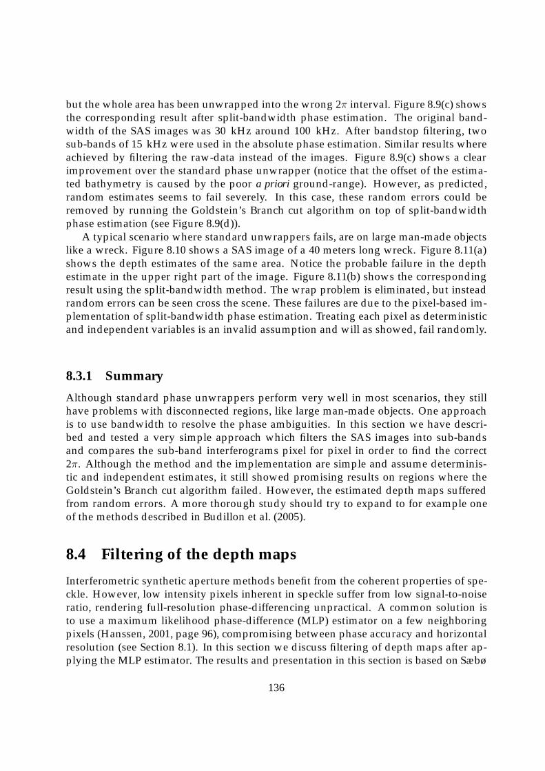
but the whole area has been unwrapped into the wrong 2π interval. Figure 8.9(c) showsthe corresponding result after split-bandwidth phase estimation. The original band-width of the SAS images was 30 kHz around 100 kHz. After bandstop filtering, twosub-bands of 15 kHz were used in the absolute phase estimation. Similar results whereachieved by filtering the raw-data instead of the images. Figure 8.9(c) shows a clearimprovement over the standard phase unwrapper (notice that the offset of the estima-ted bathymetry is caused by the poor a priori ground-range). However, as predicted,random estimates seems to fail severely. In this case, these random errors could beremoved by running the Goldstein’s Branch cut algorithm on top of split-bandwidthphase estimation (see Figure 8.9(d)).

A typical scenario where standard unwrappers fails, are on large man-made objectslike a wreck. Figure 8.10 shows a SAS image of a 40 meters long wreck. Figure 8.11(a)shows the depth estimates of the same area. Notice the probable failure in the depthestimate in the upper right part of the image. Figure 8.11(b) shows the correspondingresult using the split-bandwidth method. The wrap problem is eliminated, but insteadrandom errors can be seen cross the scene. These failures are due to the pixel-based im-plementation of split-bandwidth phase estimation. Treating each pixel as deterministicand independent variables is an invalid assumption and will as showed, fail randomly.

8.3.1 Summary

Although standard phase unwrappers perform very well in most scenarios, they stillhave problems with disconnected regions, like large man-made objects. One approachis to use bandwidth to resolve the phase ambiguities. In this section we have descri-bed and tested a very simple approach which filters the SAS images into sub-bandsand compares the sub-band interferograms pixel for pixel in order to find the correct2π. Although the method and the implementation are simple and assume determinis-tic and independent estimates, it still showed promising results on regions where theGoldstein’s Branch cut algorithm failed. However, the estimated depth maps sufferedfrom random errors. A more thorough study should try to expand to for example oneof the methods described in Budillon et al. (2005).

8.4 Filtering of the depth maps

Interferometric synthetic aperture methods benefit from the coherent properties of spe-ckle. However, low intensity pixels inherent in speckle suffer from low signal-to-noiseratio, rendering full-resolution phase-differencing unpractical. A common solution isto use a maximum likelihood phase-difference (MLP) estimator on a few neighboringpixels (Hanssen, 2001, page 96), compromising between phase accuracy and horizontalresolution (see Section 8.1). In this section we discuss filtering of depth maps after ap-plying the MLP estimator. The results and presentation in this section is based on Sæbø

136

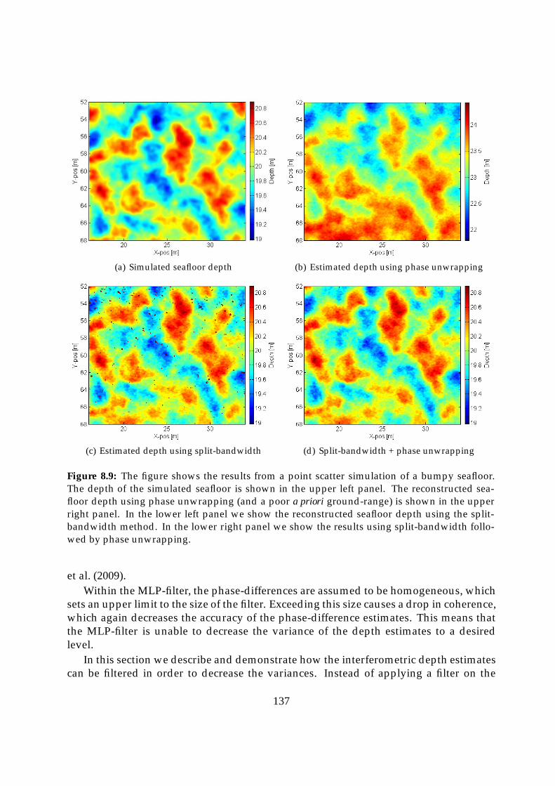
(a) Simulated seafloor depth (b) Estimated depth using phase unwrapping

(c) Estimated depth using split-bandwidth (d) Split-bandwidth + phase unwrapping

Figure 8.9: The figure shows the results from a point scatter simulation of a bumpy seafloor.The depth of the simulated seafloor is shown in the upper left panel. The reconstructed sea-floor depth using phase unwrapping (and a poor a priori ground-range) is shown in the upperright panel. In the lower left panel we show the reconstructed seafloor depth using the split-bandwidth method. In the lower right panel we show the results using split-bandwidth follo-wed by phase unwrapping.

et al. (2009).Within the MLP-filter, the phase-differences are assumed to be homogeneous, which

sets an upper limit to the size of the filter. Exceeding this size causes a drop in coherence,which again decreases the accuracy of the phase-difference estimates. This means thatthe MLP-filter is unable to decrease the variance of the depth estimates to a desiredlevel.

In this section we describe and demonstrate how the interferometric depth estimatescan be filtered in order to decrease the variances. Instead of applying a filter on the

137

Figure 8.10: The figure shows a 60 dB SAS image of a 40 meters long wreck. The data werecollected using HISAS on the HUGIN 1000-MR. The wreck is elevated 2-3 meters above theseafloor at around 30 meters water depth.

complex interferometric images we filter the depth estimates in post-processing. Thisremoves the need for homogeneous phase-differences within the filter window.

We have compared a weighted smoothing (WS) filter (Brownrigg, 1984), a weightedmedian (WM) filter (Brownrigg, 1984) and a weighted version of the bilateral (WB) filter(Tomasi and Manduchi, 1998), and found that the WB-filter performs best. The WS-filterdegrades the sharp transitions to an unacceptable degree while the WM-filter fails tosmooth flat areas sufficiently.

A very useful quantity of the interferometric processing is the coherence of the esti-mated bathymetry (Hanssen, 2001, pages 96-98) (see Section 4.7). The coherence can beconverted to an equivalent signal-to-noise ratio (see Section 4.1.3). Both the coherenceand the SNR can be employed as input weights to the filters we present. We have foundthat SNR is best suited since it better separates weights at high SNRs. In addition, weremove low SNR estimates completely by thresholding the correlation coefficient at 2/3.

138

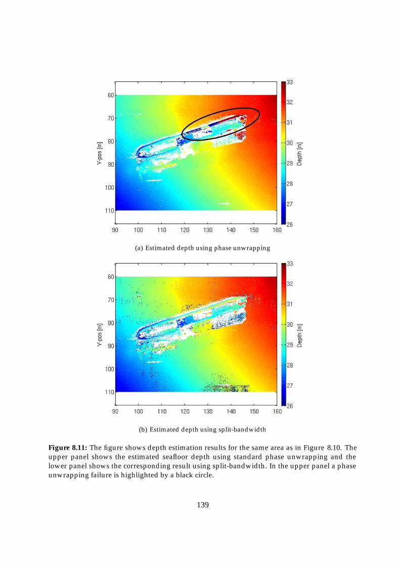
(a) Estimated depth using phase unwrapping

(b) Estimated depth using split-bandwidth

Figure 8.11: The figure shows depth estimation results for the same area as in Figure 8.10. Theupper panel shows the estimated seafloor depth using standard phase unwrapping and thelower panel shows the corresponding result using split-bandwidth. In the upper panel a phaseunwrapping failure is highlighted by a black circle.

139

We define a set of filtering weights, w

w =

{ρ : k ≥ 2/30 : k < 2/3

(8.5)

In addition we have tested the square root of SNR and the logarithm of SNR, but theyboth performed poorer than SNR itself.

8.4.1 Maximum likelihood phase-difference filter

The variances in the phase-difference estimates can be reduced by increasing the size ofthe Maximum likelihood phase-difference filter. The phase-differences are estimated by(see Section 4.5)

θ = ∠

⎧⎪⎪⎪⎪⎨⎪⎪⎪⎪⎩N∑i=1

a[i]b∗[i]√N∑i=1

|a[i]|2|b∗[i]|2

⎫⎪⎪⎪⎪⎬⎪⎪⎪⎪⎭, (8.6)

where a[i] is the i‘th pixel of the master image and b[i] is the corresponding pixel in theslave image. The relative depths, z1 are found by converting the phase-difference to aground-range translation and applying Equations 3.20. This filter is always used in theinterferometric processing, independent of subsequent filtering. The advantage withthis filter is that it is a maximum likelihood filter, but it assumes homogeneity withinthe filter size.

8.4.2 Weighted smoothing filter

The weighted smoothing filter is a weighted neighboring filter applied on the relativedepth estimates,

z2 =

∑i wizi∑i wi

, (8.7)

where w are the weights defined in Equation 8.5 and z is the original depth estimates.The weighted smoothing filter performs well on slowly varying seafloors but it de-grades edges and small objects.

8.4.3 Weighted median filter

The weighted median filter is a standard edge-preserving filter (Gonzales and Woods,1992, pages 191-195). Contrary to traditional weighted median filters, our version isimplemented with adaptive, non-integer weights. First the window depth values aresorted in ascending order. Using this sample order, the smallest index is found whose

140

cumulative weight is equal or greater than half the total weight sum. The correspondingdepth is the weighted median value.

z3 = zk, wheremin

k

{k∑

i=1

≥ 1

2

n∑i=1

}, (8.8)

where n is the number of window pixels, z are the original depths andw are weights sor-ted in ascending depth. The advantage of the weighted median-filter is that it removeswild points while preserving edges. The disadvantage is that it has an unpredictablestatistical behavior and it does not smooth slowly varying regions sufficiently.

8.4.4 Weighted bilateral filter

The weighted bilateral filter is the most complex filter. It consists of a Gaussian smoo-thing in both horizontal and vertical direction. Thus each sample is weighted accordingto three criteria: The horizontal distance from the center sample, the difference in value(vertical distance) from the center sample, and the weight

z4 =

∑iG(di)G(vi)wizi∑iG(di)G(vi)wi

, (8.9)

where d are the horizontal distances, v the differences in value andG the Gauss-functionwith standard deviation σ

G(x) =1

2πσ2exp

(− x2

2σ2

). (8.10)

The weighted bilateral filter smooths slowly varying regions while preserving edgesand therefore provides high resolution on sharp objects and less resolution on a flatseafloor. These properties are both desirable for visualization of 3D surfaces.

8.4.5 Experimental results

We have tested the different filters on a selection of experimental data collected with HI-SAS. The original bathymetry often shows an unnatural large variability on flat regionsof the seafloor, caused by a marginal SNR in the interferometric processing. On rocks orman-made objects, the reflectivity and thus the SNR are usually higher. Therefore theaccuracy of the estimated shape of objects can be much higher.

An ideal bathymetric filter should smooth slowly varying parts of the seafloor andpreserve edges, while using the coherence (or SNR) as weights to limit noise contri-butions. One approach is to change the size of the MLP filter adaptively (see Section8.1).

Figure 8.12 shows an example of the estimated bathymetry on a small part of a 30meters long wreck. Notice two different sections: The flat seafloor at the left and the

141

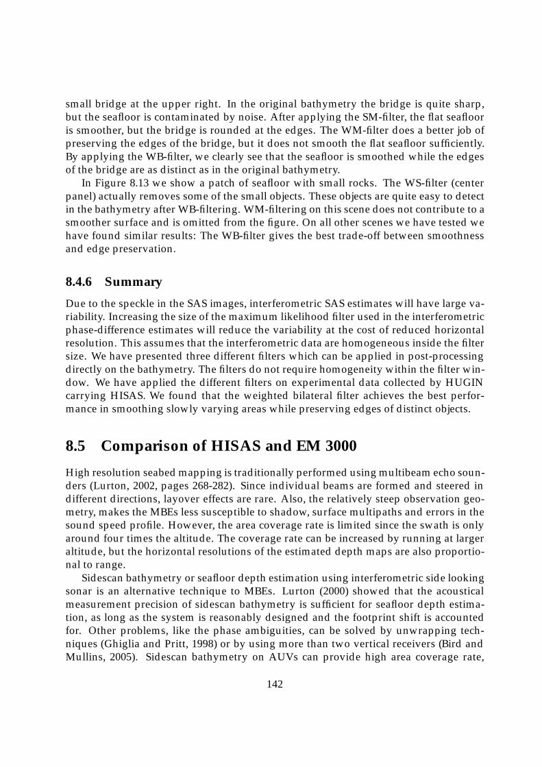
small bridge at the upper right. In the original bathymetry the bridge is quite sharp,but the seafloor is contaminated by noise. After applying the SM-filter, the flat seaflooris smoother, but the bridge is rounded at the edges. The WM-filter does a better job ofpreserving the edges of the bridge, but it does not smooth the flat seafloor sufficiently.By applying the WB-filter, we clearly see that the seafloor is smoothed while the edgesof the bridge are as distinct as in the original bathymetry.

In Figure 8.13 we show a patch of seafloor with small rocks. The WS-filter (centerpanel) actually removes some of the small objects. These objects are quite easy to detectin the bathymetry after WB-filtering. WM-filtering on this scene does not contribute to asmoother surface and is omitted from the figure. On all other scenes we have tested wehave found similar results: The WB-filter gives the best trade-off between smoothnessand edge preservation.

8.4.6 Summary

Due to the speckle in the SAS images, interferometric SAS estimates will have large va-riability. Increasing the size of the maximum likelihood filter used in the interferometricphase-difference estimates will reduce the variability at the cost of reduced horizontalresolution. This assumes that the interferometric data are homogeneous inside the filtersize. We have presented three different filters which can be applied in post-processingdirectly on the bathymetry. The filters do not require homogeneity within the filter win-dow. We have applied the different filters on experimental data collected by HUGINcarrying HISAS. We found that the weighted bilateral filter achieves the best perfor-mance in smoothing slowly varying areas while preserving edges of distinct objects.

8.5 Comparison of HISAS and EM 3000

High resolution seabed mapping is traditionally performed using multibeam echo soun-ders (Lurton, 2002, pages 268-282). Since individual beams are formed and steered indifferent directions, layover effects are rare. Also, the relatively steep observation geo-metry, makes the MBEs less susceptible to shadow, surface multipaths and errors in thesound speed profile. However, the area coverage rate is limited since the swath is onlyaround four times the altitude. The coverage rate can be increased by running at largeraltitude, but the horizontal resolutions of the estimated depth maps are also proportio-nal to range.

Sidescan bathymetry or seafloor depth estimation using interferometric side lookingsonar is an alternative technique to MBEs. Lurton (2000) showed that the acousticalmeasurement precision of sidescan bathymetry is sufficient for seafloor depth estima-tion, as long as the system is reasonably designed and the footprint shift is accountedfor. Other problems, like the phase ambiguities, can be solved by unwrapping tech-niques (Ghiglia and Pritt, 1998) or by using more than two vertical receivers (Bird andMullins, 2005). Sidescan bathymetry on AUVs can provide high area coverage rate,

142

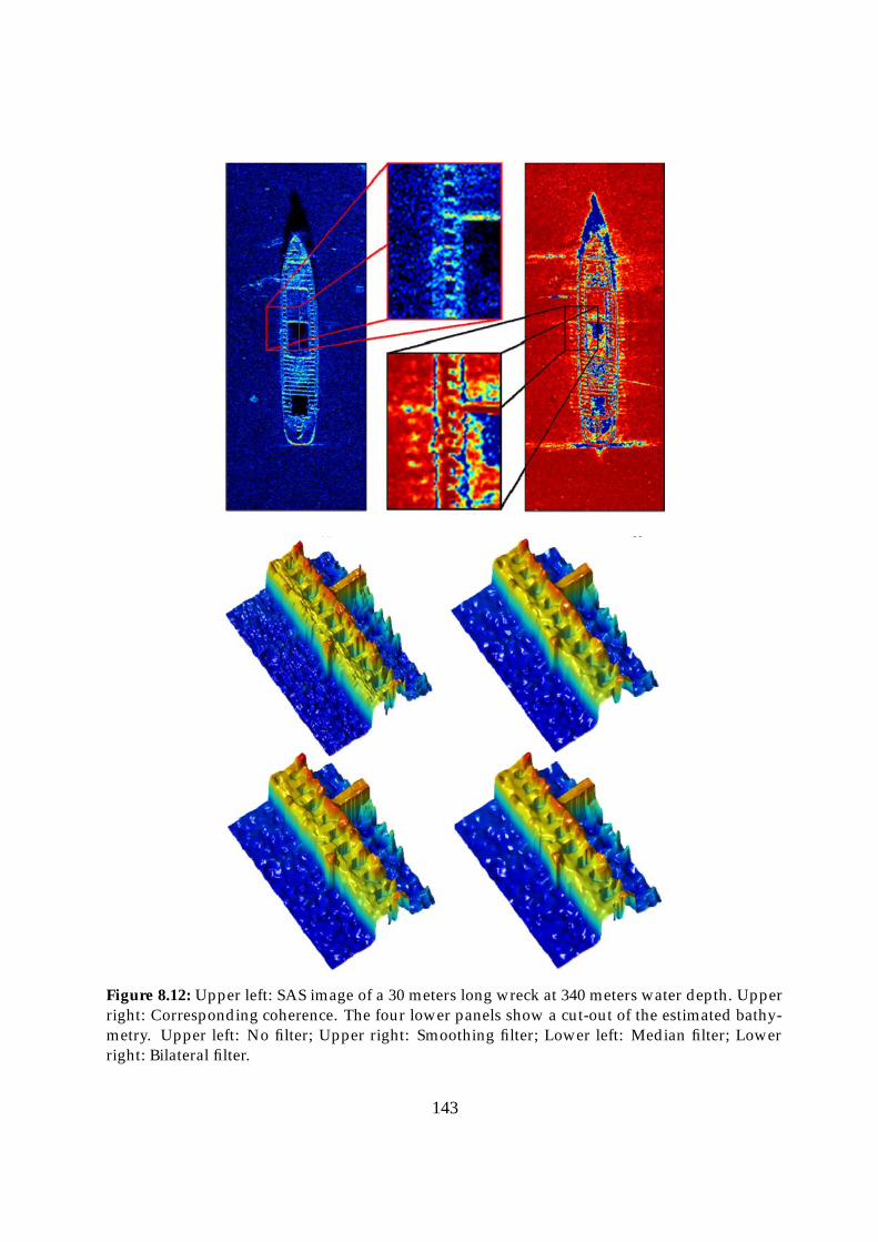
Figure 8.12: Upper left: SAS image of a 30 meters long wreck at 340 meters water depth. Upperright: Corresponding coherence. The four lower panels show a cut-out of the estimated bathy-metry. Upper left: No filter; Upper right: Smoothing filter; Lower left: Median filter; Lowerright: Bilateral filter.

143

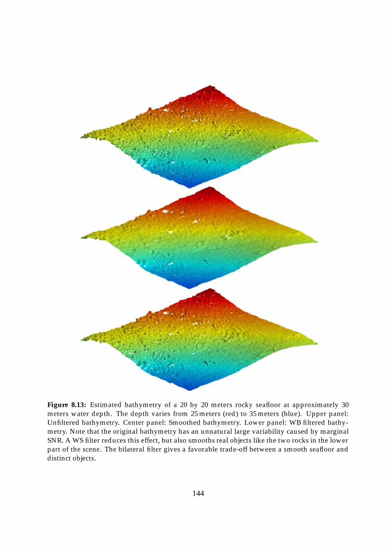
Figure 8.13: Estimated bathymetry of a 20 by 20 meters rocky seafloor at approximately 30meters water depth. The depth varies from 25 meters (red) to 35 meters (blue). Upper panel:Unfiltered bathymetry. Center panel: Smoothed bathymetry. Lower panel: WB filtered bathy-metry. Note that the original bathymetry has an unnatural large variability caused by marginalSNR. A WS filter reduces this effect, but also smooths real objects like the two rocks in the lowerpart of the scene. The bilateral filter gives a favorable trade-off between a smooth seafloor anddistinct objects.

144

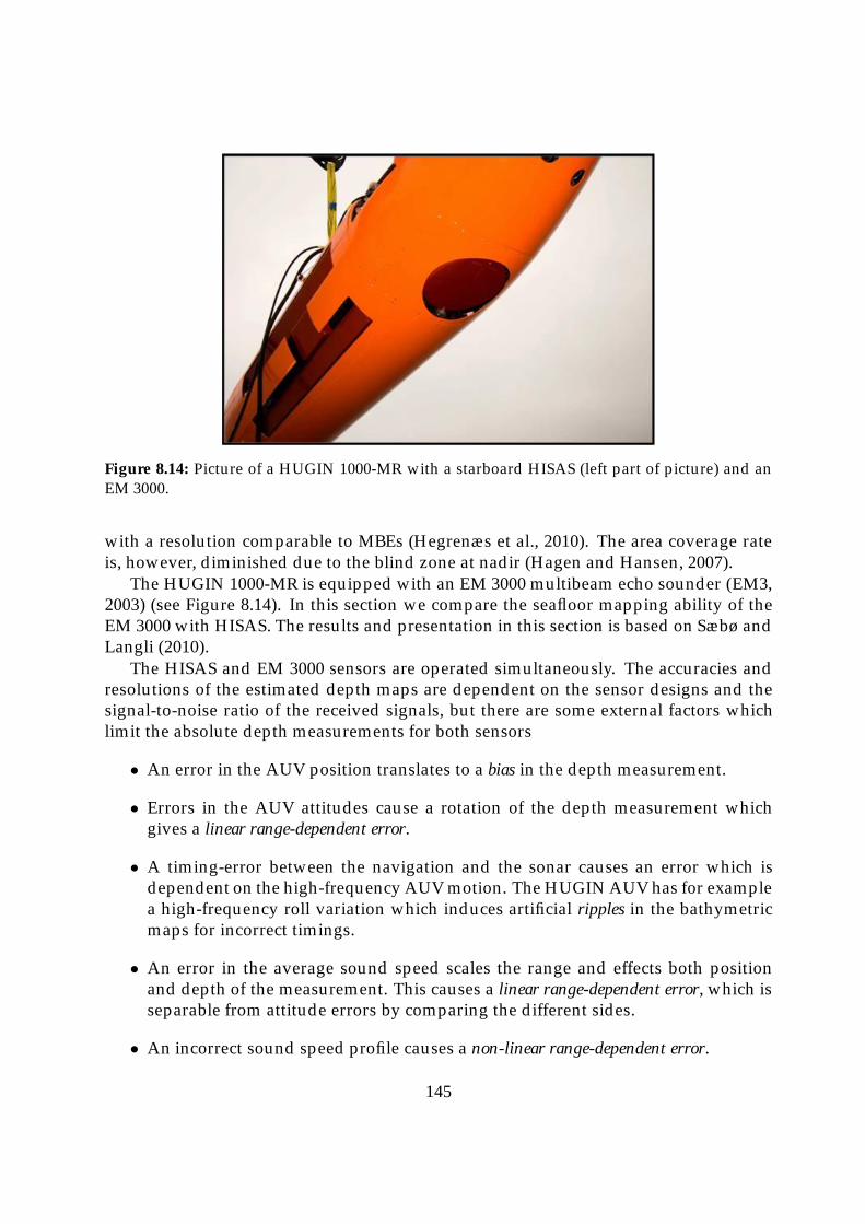
Figure 8.14: Picture of a HUGIN 1000-MR with a starboard HISAS (left part of picture) and anEM 3000.

with a resolution comparable to MBEs (Hegrenæs et al., 2010). The area coverage rateis, however, diminished due to the blind zone at nadir (Hagen and Hansen, 2007).

The HUGIN 1000-MR is equipped with an EM 3000 multibeam echo sounder (EM3,2003) (see Figure 8.14). In this section we compare the seafloor mapping ability of theEM 3000 with HISAS. The results and presentation in this section is based on Sæbø andLangli (2010).

The HISAS and EM 3000 sensors are operated simultaneously. The accuracies andresolutions of the estimated depth maps are dependent on the sensor designs and thesignal-to-noise ratio of the received signals, but there are some external factors whichlimit the absolute depth measurements for both sensors

• An error in the AUV position translates to a bias in the depth measurement.

• Errors in the AUV attitudes cause a rotation of the depth measurement whichgives a linear range-dependent error.

• A timing-error between the navigation and the sonar causes an error which isdependent on the high-frequency AUV motion. The HUGIN AUV has for examplea high-frequency roll variation which induces artificial ripples in the bathymetricmaps for incorrect timings.

• An error in the average sound speed scales the range and effects both positionand depth of the measurement. This causes a linear range-dependent error, which isseparable from attitude errors by comparing the different sides.

• An incorrect sound speed profile causes a non-linear range-dependent error.

145

Figure 8.15: Sketch of the sensor geometry on board the HUGIN AUV. The orange circle illus-trates a cross-section of the AUV, the gray area the HISAS swath and the green and red areasthe EM 3000 swath. While HISAS uses time-difference of arrival (TDOA) to locate the seafloordepth, the EM switches between time of arrival (TOA) (red area) and TDOA (green area).

• An error in the internal lever-arms (e.g. the distance from the navigation unit tothe sensor) will cause an attitude dependent bias.

It is fairly easy to calibrate range-dependent errors by inspecting the estimated bathy-metries of overlapping regions in a lawn-mower pattern. A timing error can be detectedby correlating along-track seafloor variations with short-time AUV attitudes. The mostchallenging errors are errors in the AUV position and internal lever-arm errors.

8.5.1 The EM 3000

The EM 3000 (EM3, 2003) is a 300 kHz high-resolution multibeam echo sounder for sea-bed mapping and inspection (Lurton, 2002, pages 268-282). Its depth rating and phy-sical dimensions makes it well suited for use on HUGIN AUVs. The swath-width of130 degrees provides ground-range coverage up to four times the sensor altitude. Theangular resolution is obtained using the Mills cross principle (Urick, 1983, page 62), andthe beamwidths of the 127 beams ranges from 1.5 degrees at the vertical to 3.5 degreesat ±65 degrees. For beams having close to normal incidence, the range is typically de-termined by a center of gravity amplitude detection principle (or time of arrival, seeFigure 8.15). For more horizontal geometries, the echoes from the seafloor are less well-defined and amplitude detection can only provide coarse range estimates. Range atthe beam pointing angles are then found using the split-beam technique (Burdic, 1984,pages 327-331): the receiver array is divided into two subarrays, for each subarray abeam is computed, and range is found comparing the phase of the two half-beams andidentifying the instant of zero phase-difference. The last step is almost identical to theinterferometric processing on HISAS. With good external sensors, the system deliversbathymetry with precision of 5 cm RMS in shallow water.

When HISAS is operated in SAS mode the sampling criterion limits the speed of theAUV. A typical velocity is around 2 m/s, which at 20 meters altitude gives a theoreticalarea coverage rate of 0.6 km2/h for the EM. However, when SAS processing is not en-

146

abled, the speed of the vehicle can be increased. For the HUGIN 1000-MR the maximumoperating speed is around 3 m/s, which at 20 meters altitude results in a mapping rateof 0.9 km2/h. Additional increase in the rate can be made by increasing the altitude.However, at some point the resolution becomes too poor, the range too large or the pingspacing too separated. A reasonable altitude is 40 meters which gives the EM an areacoverage rate of 1.7 km2/h. In comparison, a typical area coverage rate for HISAS is1.8 km2/h (Hagen and Hansen, 2007).

8.5.2 Large scale comparison between EM 3000 and HISAS

In Figure 8.16 we present results from a shallow water survey in January 2009. The dataare collected outside Horten of Norway, where the water depth varies between 10 and20 meters. The AUV has run in a lawn-mower pattern seven meters above the seafloor.In the figure we show the aligned bathymetry for the EM 3000 and for HISAS. We alsoshow the differences between the two depth maps.

The difference in area coverage rate is clearly seen by comparing the upper panelsof Figure 8.16. In addition to the increase in the surveyed area, HISAS has been runwith heavy overlap and each area of the seafloor is observed four times. This is done toensure full coverage with the EM.

The bathymetric maps in Figure 8.16 seem to agree very well, but the lower panel ofthe figure shows that there are differences. There is both a small bias of 15.7 cm and asmall systematic discrepancy. We have seen similar bias at deep waters with flat seafloorand a constant sound speed profile and believe that the bias is caused by an erroneouslever-arm on one of the systems. This theory is strengthened from observations wherethe apparent bias changes when the vehicle pitches.

The systematic error (seen as an cross-track pattern in the lower panel of Figure 8.16)is less dominant than the bias and can either be caused by a lever-arm error or by anincorrect sound speed profile. The estimated sound speed profile varies with approxi-mately 0.1 percent from the position of the AUV down to the seafloor. A linear errorin the profile of 0.01 percent will cause a depth-error of 5 cm at 85 meters range. Thestandard deviation of the differences between the bathymetric maps is only 1.7 cm, soignoring the bias, the two sensors produce almost identical depth maps. The differencein frequency gives a different penetration level, so for some types of seafloor the sen-sors should disagree. Also, the resolution difference will contribute to a small standarddeviation in the differences.

In Figure 8.17 we investigate the two bathymetries in Figure 8.16 in more detail.The upper right panel shows a horizontal slice through the two depth maps and thelower panel shows a vertical slice. The location of the slices are shown in the upperleft panel. Both slices illustrate that the agreement between EM 3000 bathymetry andHISAS bathymetry is excellent, after accounting for the bias of approximately 15 cm.

147

Figure 8.16: Comparison of EM 3000 depth estimates and HISAS depth estimates for a shallowwater survey outside Horten in January 2009. The upper left panel shows the geo-referenceddepth measurements using the EM 3000. The black line shows the AUV trajectory. Notice thatthere are small gaps in the depth map due to the limited swath-width of the EM 3000. The upperright panel shows the estimates using HISAS, collected simultaneously. Notice that the coverageis significantly increased. The lower panel shows the difference between the two depth maps.The average difference is 15.7 cm while the standard deviation of the difference is 1.7 cm. Noticethat there is a small but systematic cross-track discrepancy.

148

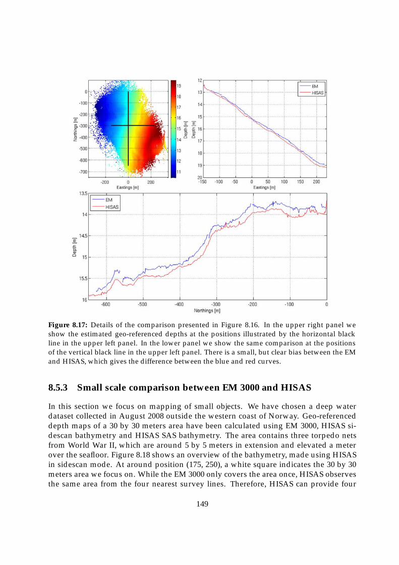
Figure 8.17: Details of the comparison presented in Figure 8.16. In the upper right panel weshow the estimated geo-referenced depths at the positions illustrated by the horizontal blackline in the upper left panel. In the lower panel we show the same comparison at the positionsof the vertical black line in the upper left panel. There is a small, but clear bias between the EMand HISAS, which gives the difference between the blue and red curves.

8.5.3 Small scale comparison between EM 3000 and HISAS

In this section we focus on mapping of small objects. We have chosen a deep waterdataset collected in August 2008 outside the western coast of Norway. Geo-referenceddepth maps of a 30 by 30 meters area have been calculated using EM 3000, HISAS si-descan bathymetry and HISAS SAS bathymetry. The area contains three torpedo netsfrom World War II, which are around 5 by 5 meters in extension and elevated a meterover the seafloor. Figure 8.18 shows an overview of the bathymetry, made using HISASin sidescan mode. At around position (175, 250), a white square indicates the 30 by 30meters area we focus on. While the EM 3000 only covers the area once, HISAS observesthe same area from the four nearest survey lines. Therefore, HISAS can provide four

149

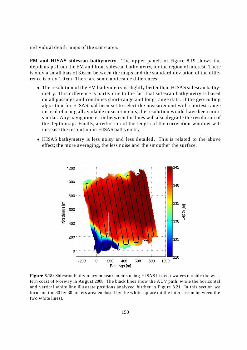
individual depth maps of the same area.

EM and HISAS sidescan bathymetry The upper panels of Figure 8.19 shows thedepth maps from the EM and from sidescan bathymetry, for the region of interest. Thereis only a small bias of 3.6 cm between the maps and the standard deviation of the diffe-rence is only 1.0 cm. There are some noticeable differences:

• The resolution of the EM bathymetry is slightly better than HISAS sidescan bathy-metry. This difference is partly due to the fact that sidescan bathymetry is basedon all passings and combines short-range and long-range data. If the geo-codingalgorithm for HISAS had been set to select the measurement with shortest rangeinstead of using all available measurements, the resolution would have been moresimilar. Any navigation error between the lines will also degrade the resolution ofthe depth map. Finally, a reduction of the length of the correlation window willincrease the resolution in HISAS bathymetry.

• HISAS bathymetry is less noisy and less detailed. This is related to the aboveeffect; the more averaging, the less noise and the smoother the surface.

Figure 8.18: Sidescan bathymetry measurements using HISAS in deep waters outside the wes-tern coast of Norway in August 2008. The black lines show the AUV path, while the horizontaland vertical white line illustrate positions analyzed further in Figure 8.21. In this section wefocus on the 30 by 30 meters area enclosed by the white square (at the intersection between thetwo white lines).

150

Figure 8.19: Details of the area highlighted in Figure 8.18. The upper left panel shows a depthmap using EM 3000 measurements and the upper right panel the same using HISAS in sidescanmode. The depths are shown in a common grid. The mean difference between the depth mapsis 3.6 cm while the standard deviation of the difference is 1.0 cm. The center left panel shows theSAS image for pass #1 and the lower left panel the SAS image for pass #4. The correspondingright panels show the depth maps estimated using SAS interferometry. The bias between theEM depth and the depth from pass #1 is -32 cm, while the bias between EM and pass #4 is 52 cm.All the biases are subtracted in the figure.

151

HISAS SAS bathymetry The lower left panels in Figure 8.19 show SAS images fromtwo sides of the area, both with a range of above 100 meters. The lower right panelsshow the corresponding SAS bathymetries. From the SAS images it is clear that theacoustic echo looks quite different from each side. This is due to the small depressionangle, which causes shadowing and layover effects. This is also reflected in the SASbathymetries. Different parts of the objects are mapped for each side and to avoid holesin the bathymetry we have to combine the bathymetries from the two sides.

The SAS bathymetries in Figure 8.19 have a bias relative to the EM bathymetry of-32 cm and 52 cm, respectively. To investigate if these biases are related to the SAS inter-ferometry method, we have made depth maps from the same passings using sidescanbathymetry. In Figure 8.20 we show the individual depth maps from the four passings.In the figure, all biases are subtracted, but relative to the EM the biases are -34 cm, -4 cm,7 cm and 47 cm for passings #1-4. These observations are presented more clearly in Fi-gure 8.21 where two cross-sections of each depth map are shown. Apparently, there is adrift in the estimated depths using HISAS, relative to the depth map from EM. We haveconsidered some of the possible causes for this drift:

• A roll error is unlikely since this would have been visible as linear errors in theright panel of Figure 8.21.

• An error in the average sound speed speed is unlikely since this also would havebeen visible in the right panel of Figure 8.21.

• An incorrect sound speed profile in unlikely since the sound speed is more or lessconstant at 330 meters water depth.

• It is not a timing-error or an internal lever-arm error since these errors do not causea drifting depth-error.

There is one plausible explanation for the biases: An erroneous drift in the estimatedAUV-position. In the region of interest at the time of the data-collection the tide canexplain some of the drift, but not all. An error in the depth of the AUV of the relevantscale is, however, within the reported accuracy of the navigation system. A thoroughinvestigation of the depth accuracy of the AUV and other causes for the drift in thedepth are outside the scope of this thesis.

Ignoring the discussed biases, Figure 8.20 shows an excellent agreement betweenthe individual depth maps. There are visible differences, but this should be expectedconsidering that the views are from two different sides and two different ranges. Thepositions of the objects seem to be quite similar, indicating that there is no apparenthorizontal drift in the AUV navigation.

8.5.4 Summary

This section is a summary of preliminary studies into the performance of seafloor map-ping using HISAS SAS. As a benchmark sensor, we have chosen an EM 3000, which

152

Figure 8.20: Details of the area highlighted in Figure 8.18. The panels show depth maps usingHISAS sidescan bathymetry. The upper left panel shows the map from pass #1, the upper rightfrom pass #2, the lower left from pass #3 and the lower right from pass #4. In the upper panelsthe area is observed from below (high y-position), in the lower panels, the area is observed fromabove. Pass #1 and #4 are observed from long range (around 100 m) while pass #2 and #3 areobserved from shorter range. The blank areas in pass #2 and #3 are to close to nadir (less than45 degrees). Notice a phase wrap error at close range in pass #3. The biases between each passare subtracted in the figure. The altitude of the AUV was 25 meters in all four passings.

through experience has proven to be a reliable and accurate mapping sensor. A studyof the theoretical performance show that the depth accuracy of the two systems is simi-lar. When it comes to horizontal resolution, the EM has slightly better, but comparableperformance to sidescan bathymetry processed HISAS data. On the other hand, HISAShas a considerable larger area coverage rate. Since the swaths of the two sensors arealmost non-overlapping, combining these two sensors together make a very efficientmapping system.

153

Figure 8.21: Details of the positions highlighted in Figure 8.18. The left panel shows the estima-ted geo-referenced depths using sidescan bathymetry at the positions illustrated by the verticalwhite line in Figure 8.18. The right panel shows the same comparison at the positions of thehorizontal white line. The average depths are shown in black, while the colored curves showthe depth for each individual pass. Clearly, there is a bias on pass #1 and #4.

The SAS bathymetry processed HISAS data has approximately the same area cove-rage, and a much higher horizontal resolution. The computational burden in full-swathSAS bathymetry is large, but SAS bathymetry on selected regions is an excellent classi-fication aid.

We have investigated the actual performance on two different sets of data. The firstsurvey took place at shallow water where we compared geo-referenced depth maps ofa one km2 area using HISAS sidescan bathymetry and EM bathymetry. The depth mapsshowed very good agreement, but we found a small bias and a small cross-track error.These are most likely caused by an external lever-arm error on one of the systems.

The second survey was a deep water survey where we looked in more detail at thedifferences between HISAS and EM bathymetry. In this case we found no significantbias, but we noticed that the depth of the selected region were drifting as a functionof time for HISAS. After eliminating a number of different error-sources, we found itlikely that this drift is caused by an error in the AUV-position. Disregarding the drift,the performance of the two sensors was as expected from the specifications. Also onsmaller objects, the EM and HISAS can be used as one combined system.

We also compared the EM and HISAS sidescan bathymetry depth maps to HISASSAS bathymetry depth maps and found that the resolutions of the SAS bathymetrydepth maps are superior. Due to the combination of high resolution and small depres-sion angle, SAS bathymetry is more susceptible to shadowing and layover. CombiningSAS bathymetry from two sides will efficiently combat this effect at the expense of re-duced area coverage rate.

154

8.6 Using HISAS for pipeline surveying

In this section, we investigate how to use interferometric SAS in pipeline inspection.The results and presentation in this section is based on Sæbø et al. (2010) and Hansenet al. (2010b). Pipeline inspection is usually performed by using a short-range sensorclose to the pipeline, which gives limited information about the surroundings. By usingan interferometric SAS, a large area including the pipeline can be mapped and imagedin one swath. In June 2009 the Royal Norwegian Navy performed a survey outside thewestern coast of Norway using HISAS on an HUGIN 1000-MR. The main purpose ofthe mission was to survey an area with a pipeline, exposed, partly exposed and buried.The particular pipeline has an inner diameter of 12′′ ≈ 30 cm, and known position priorto the mission.

A pipeline inspection survey with imaging sonar may contain the following tasks(Gauer et al., 1999)

• Detection of burial for exposed pipelines

• Detection of exposure for buried pipelines

• Detection of pipeline free span and estimation of span

• Detection of damages of pipelines

• Detection of buckling of pipelines

• Detection of debris near the pipeline

For long automated AUV surveys and short range sensors, tracking of the pipeline (Pe-tillot et al., 2002) might be mandatory. With the swath width of HISAS and the naviga-tion accuracy of the HUGIN AUV, tracking actually only becomes important for multi-hour missions (given that the pipeline position is known). In this section, we focus onthe sensor, interferometric SAS, and the particular benefits and challenges in inspectionof the pipeline and the area around.

Figure 8.22 shows an overview of the HUGIN mission. The color-coded bathymetryis estimated using HISAS sidescan bathymetry. The water depth varies from 200 to 400meters in the test area. The tracks are shown in black and the pipeline in brown. Wefocus on two different areas from this mission: Area A and Area B as indicated by thetwo squares. Figure 8.23 shows a sidescan sonar image from one mission line from oneof the sides. Note that the pipeline is covered by gravel in several locations.

In Area B the AUV runs parallel to the pipeline at around 60 meters range to bothsides. We have co-registered (Jakowatz et al., 1996, 288-302) data from the two sides andmerged SAS images and SAS bathymetries. The results are presented in Section 8.6.1.In Area A the AUV has run perpendicular to the pipeline and passed directly above it.Processed data from Area A are presented in Section 8.6.2. In Section 8.6.3 we presentresults from shape estimation of the pipeline from both datasets.

155

Figure 8.22: Overview of the pipeline mission. The data are collected by the Royal NorwegianNavy, outside the western coast of Norway

156

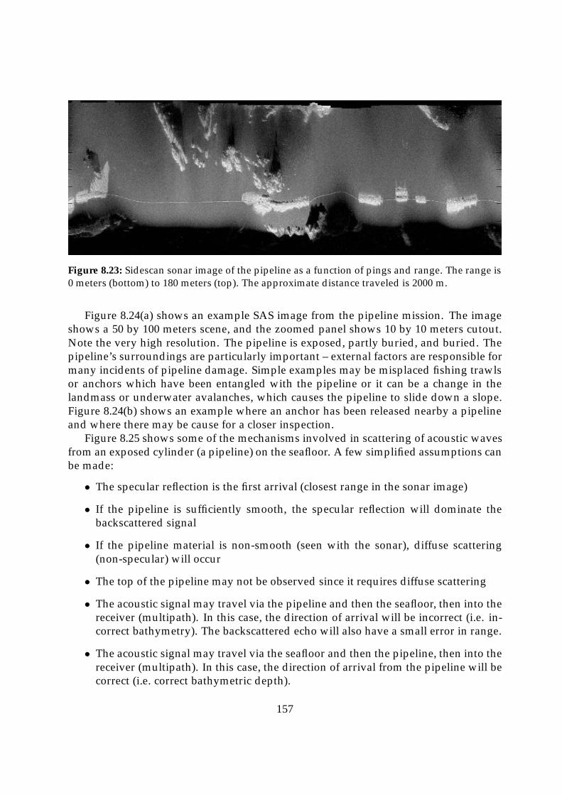
Figure 8.23: Sidescan sonar image of the pipeline as a function of pings and range. The range is0 meters (bottom) to 180 meters (top). The approximate distance traveled is 2000 m.

Figure 8.24(a) shows an example SAS image from the pipeline mission. The imageshows a 50 by 100 meters scene, and the zoomed panel shows 10 by 10 meters cutout.Note the very high resolution. The pipeline is exposed, partly buried, and buried. Thepipeline’s surroundings are particularly important – external factors are responsible formany incidents of pipeline damage. Simple examples may be misplaced fishing trawlsor anchors which have been entangled with the pipeline or it can be a change in thelandmass or underwater avalanches, which causes the pipeline to slide down a slope.Figure 8.24(b) shows an example where an anchor has been released nearby a pipelineand where there may be cause for a closer inspection.

Figure 8.25 shows some of the mechanisms involved in scattering of acoustic wavesfrom an exposed cylinder (a pipeline) on the seafloor. A few simplified assumptions canbe made:

• The specular reflection is the first arrival (closest range in the sonar image)

• If the pipeline is sufficiently smooth, the specular reflection will dominate thebackscattered signal

• If the pipeline material is non-smooth (seen with the sonar), diffuse scattering(non-specular) will occur

• The top of the pipeline may not be observed since it requires diffuse scattering

• The acoustic signal may travel via the pipeline and then the seafloor, then into thereceiver (multipath). In this case, the direction of arrival will be incorrect (i.e. in-correct bathymetry). The backscattered echo will also have a small error in range.

• The acoustic signal may travel via the seafloor and then the pipeline, then into thereceiver (multipath). In this case, the direction of arrival from the pipeline will becorrect (i.e. correct bathymetric depth).

157

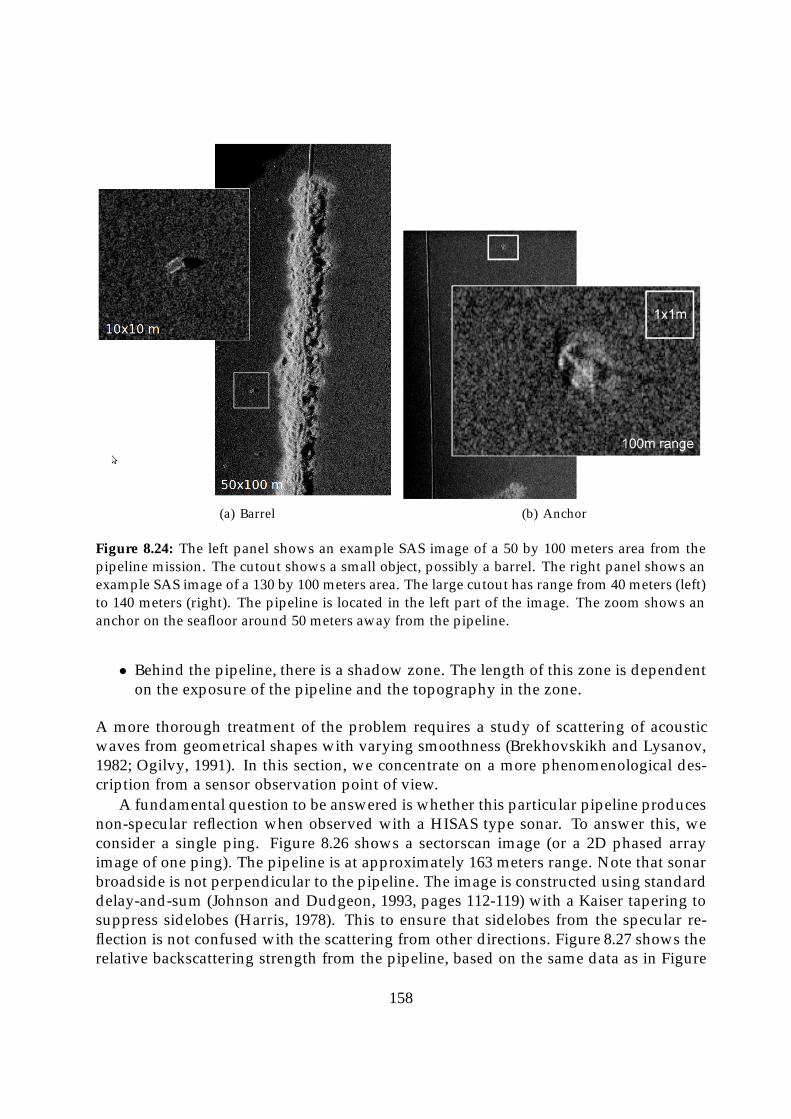
(a) Barrel (b) Anchor

Figure 8.24: The left panel shows an example SAS image of a 50 by 100 meters area from thepipeline mission. The cutout shows a small object, possibly a barrel. The right panel shows anexample SAS image of a 130 by 100 meters area. The large cutout has range from 40 meters (left)to 140 meters (right). The pipeline is located in the left part of the image. The zoom shows ananchor on the seafloor around 50 meters away from the pipeline.

• Behind the pipeline, there is a shadow zone. The length of this zone is dependenton the exposure of the pipeline and the topography in the zone.

A more thorough treatment of the problem requires a study of scattering of acousticwaves from geometrical shapes with varying smoothness (Brekhovskikh and Lysanov,1982; Ogilvy, 1991). In this section, we concentrate on a more phenomenological des-cription from a sensor observation point of view.

A fundamental question to be answered is whether this particular pipeline producesnon-specular reflection when observed with a HISAS type sonar. To answer this, weconsider a single ping. Figure 8.26 shows a sectorscan image (or a 2D phased arrayimage of one ping). The pipeline is at approximately 163 meters range. Note that sonarbroadside is not perpendicular to the pipeline. The image is constructed using standarddelay-and-sum (Johnson and Dudgeon, 1993, pages 112-119) with a Kaiser tapering tosuppress sidelobes (Harris, 1978). This to ensure that sidelobes from the specular re-flection is not confused with the scattering from other directions. Figure 8.27 shows therelative backscattering strength from the pipeline, based on the same data as in Figure

158

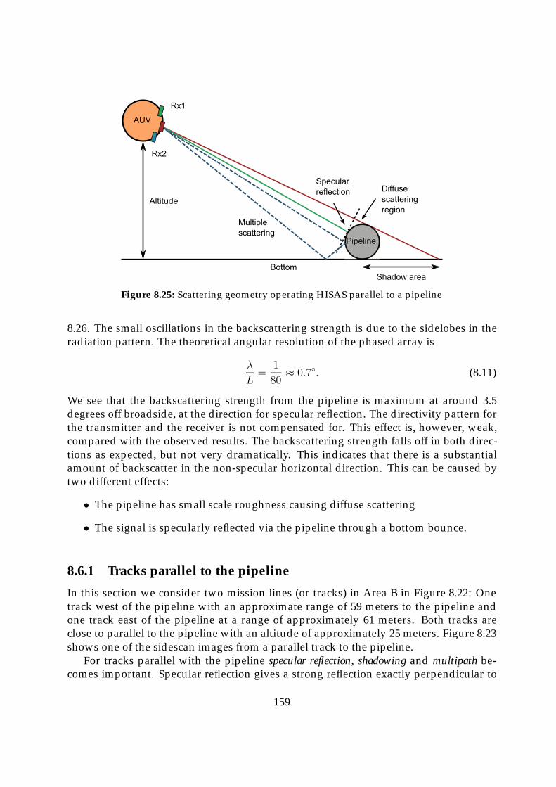
Bottom

Altitude

Rx1

Rx2

AUV

Shadow area

Specularreflection Diffuse

scatteringregion

Multiplescattering

Figure 8.25: Scattering geometry operating HISAS parallel to a pipeline

8.26. The small oscillations in the backscattering strength is due to the sidelobes in theradiation pattern. The theoretical angular resolution of the phased array is

λ

L=

1

80≈ 0.7◦. (8.11)

We see that the backscattering strength from the pipeline is maximum at around 3.5degrees off broadside, at the direction for specular reflection. The directivity pattern forthe transmitter and the receiver is not compensated for. This effect is, however, weak,compared with the observed results. The backscattering strength falls off in both direc-tions as expected, but not very dramatically. This indicates that there is a substantialamount of backscatter in the non-specular horizontal direction. This can be caused bytwo different effects:

• The pipeline has small scale roughness causing diffuse scattering

• The signal is specularly reflected via the pipeline through a bottom bounce.

8.6.1 Tracks parallel to the pipeline

In this section we consider two mission lines (or tracks) in Area B in Figure 8.22: Onetrack west of the pipeline with an approximate range of 59 meters to the pipeline andone track east of the pipeline at a range of approximately 61 meters. Both tracks areclose to parallel to the pipeline with an altitude of approximately 25 meters. Figure 8.23shows one of the sidescan images from a parallel track to the pipeline.

For tracks parallel with the pipeline specular reflection, shadowing and multipath be-comes important. Specular reflection gives a strong reflection exactly perpendicular to

159

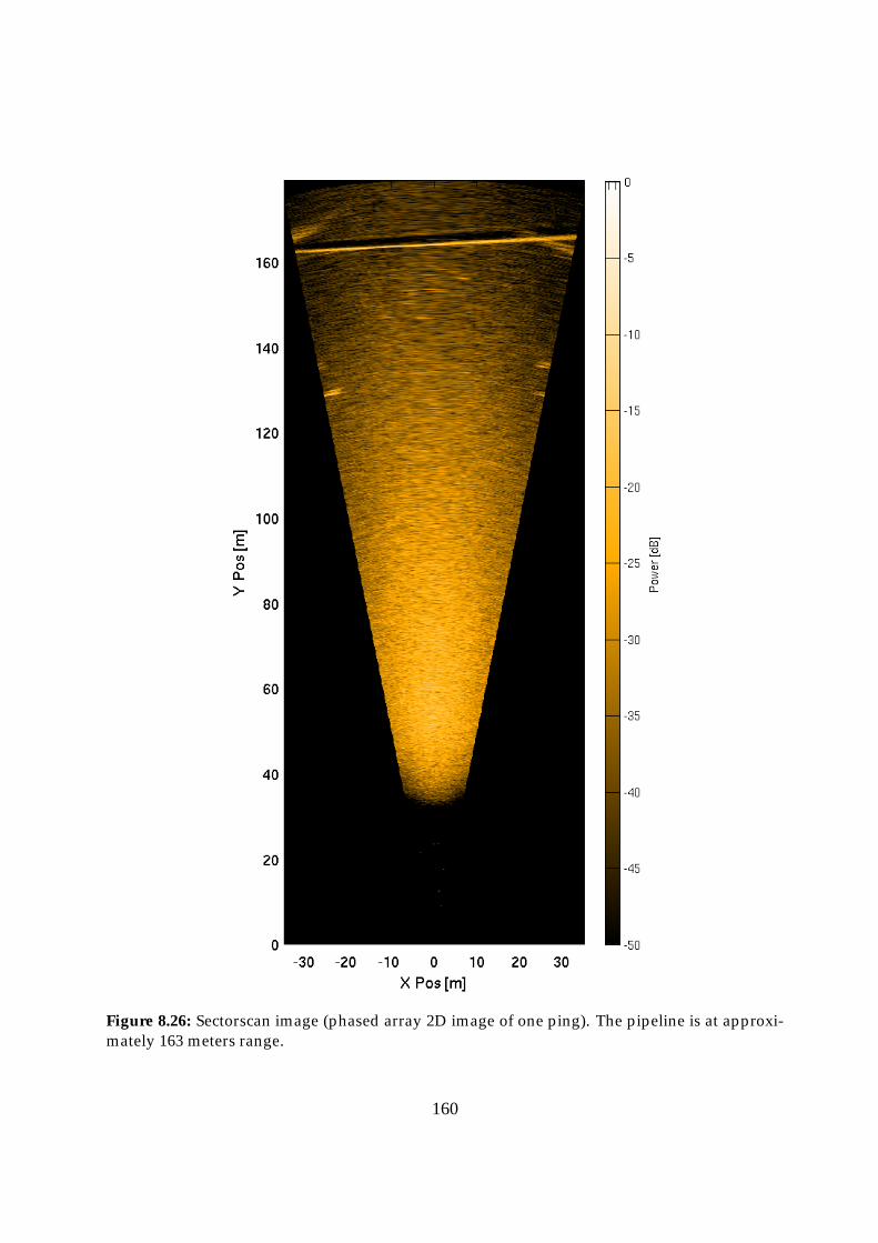
Figure 8.26: Sectorscan image (phased array 2D image of one ping). The pipeline is at approxi-mately 163 meters range.

160

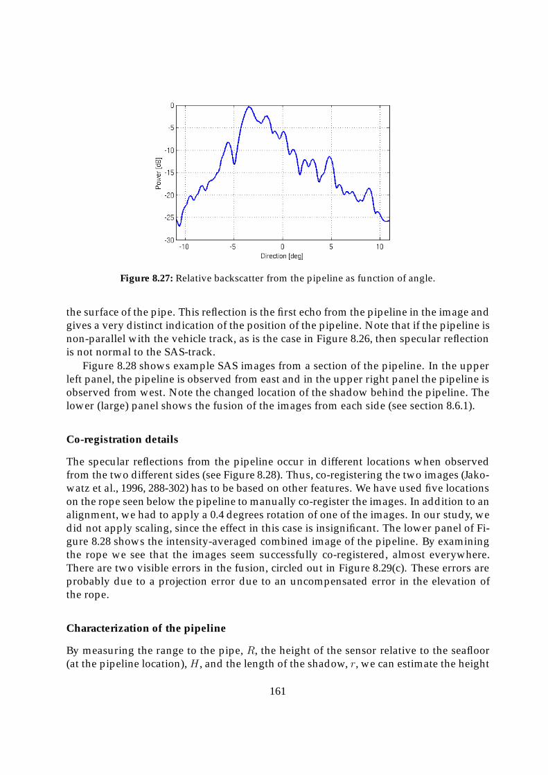
Figure 8.27: Relative backscatter from the pipeline as function of angle.

the surface of the pipe. This reflection is the first echo from the pipeline in the image andgives a very distinct indication of the position of the pipeline. Note that if the pipeline isnon-parallel with the vehicle track, as is the case in Figure 8.26, then specular reflectionis not normal to the SAS-track.

Figure 8.28 shows example SAS images from a section of the pipeline. In the upperleft panel, the pipeline is observed from east and in the upper right panel the pipeline isobserved from west. Note the changed location of the shadow behind the pipeline. Thelower (large) panel shows the fusion of the images from each side (see section 8.6.1).

Co-registration details

The specular reflections from the pipeline occur in different locations when observedfrom the two different sides (see Figure 8.28). Thus, co-registering the two images (Jako-watz et al., 1996, 288-302) has to be based on other features. We have used five locationson the rope seen below the pipeline to manually co-register the images. In addition to analignment, we had to apply a 0.4 degrees rotation of one of the images. In our study, wedid not apply scaling, since the effect in this case is insignificant. The lower panel of Fi-gure 8.28 shows the intensity-averaged combined image of the pipeline. By examiningthe rope we see that the images seem successfully co-registered, almost everywhere.There are two visible errors in the fusion, circled out in Figure 8.29(c). These errors areprobably due to a projection error due to an uncompensated error in the elevation ofthe rope.

Characterization of the pipeline

By measuring the range to the pipe, R, the height of the sensor relative to the seafloor(at the pipeline location), H , and the length of the shadow, r, we can estimate the height

161

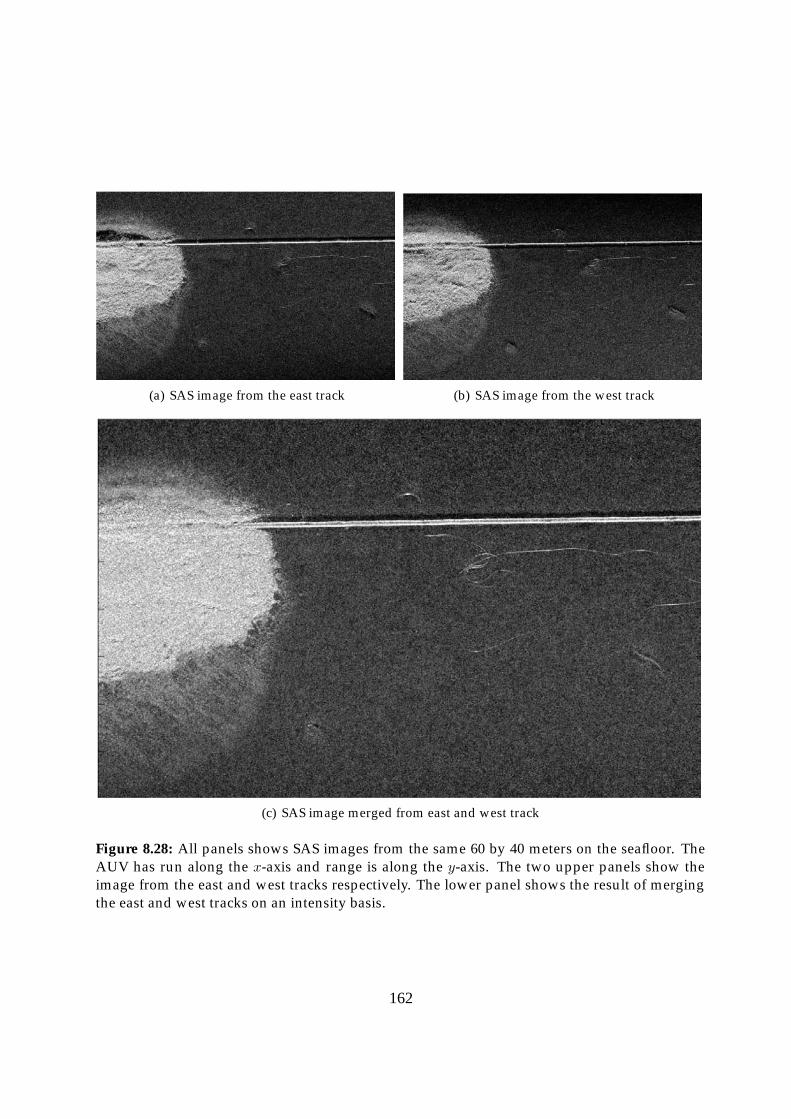
(a) SAS image from the east track (b) SAS image from the west track

(c) SAS image merged from east and west track

Figure 8.28: All panels shows SAS images from the same 60 by 40 meters on the seafloor. TheAUV has run along the x-axis and range is along the y-axis. The two upper panels show theimage from the east and west tracks respectively. The lower panel shows the result of mergingthe east and west tracks on an intensity basis.

162

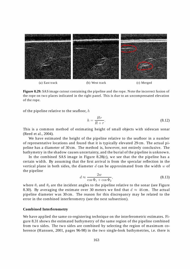
(a) East track (b) West track (c) Merged

Figure 8.29: SAS image cutout containing the pipeline and the rope. Note the incorrect fusion ofthe rope on two places indicated in the right panel. This is due to an uncompensated elevationof the rope.

of the pipeline relative to the seafloor, h

h =Hr

R + r. (8.12)

This is a common method of estimating height of small objects with sidescan sonar(Reed et al., 2004).

We have estimated the height of the pipeline relative to the seafloor in a numberof representative locations and found that it is typically elevated 29 cm. The actual pi-peline has a diameter of 30 cm. The method is, however, not entirely conclusive. Thebathymetry in the shadow causes uncertainty, and the burial of the pipeline is unknown.

In the combined SAS image in Figure 8.28(c), we see that the the pipeline has acertain width. By assuming that the first arrival is from the specular reflection in thevertical plane in both sides, the diameter d can be approximated from the width w ofthe pipeline

d ≈ 2w

cosΦ1 + cosΦ2, (8.13)

where θ1 and θ2 are the incident angles to the pipeline relative to the sonar (see Figure8.30). By averaging the estimate over 30 meters we find that d ≈ 46 cm. The actualpipeline diameter was 30 cm. The reason for this discrepancy may be related to theerror in the combined interferometry (see the next subsection).

Combined Interferometry

We have applied the same co-registering technique on the interferometric estimates. Fi-gure 8.31 shows the estimated bathymetry of the same region of the pipeline combinedfrom two sides. The two sides are combined by selecting the region of maximum co-herence (Hanssen, 2001, pages 96-98) in the two single-look bathymetries, i.e. there is

163

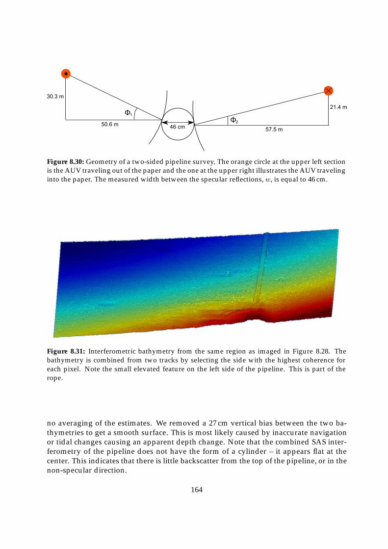
30.3 m

21.4 m

50.6 m57.5 m

Φ1Φ2

46 cm

Figure 8.30: Geometry of a two-sided pipeline survey. The orange circle at the upper left sectionis the AUV traveling out of the paper and the one at the upper right illustrates the AUV travelinginto the paper. The measured width between the specular reflections, w, is equal to 46 cm.

Figure 8.31: Interferometric bathymetry from the same region as imaged in Figure 8.28. Thebathymetry is combined from two tracks by selecting the side with the highest coherence foreach pixel. Note the small elevated feature on the left side of the pipeline. This is part of therope.

no averaging of the estimates. We removed a 27 cm vertical bias between the two ba-thymetries to get a smooth surface. This is most likely caused by inaccurate navigationor tidal changes causing an apparent depth change. Note that the combined SAS inter-ferometry of the pipeline does not have the form of a cylinder – it appears flat at thecenter. This indicates that there is little backscatter from the top of the pipeline, or in thenon-specular direction.

164

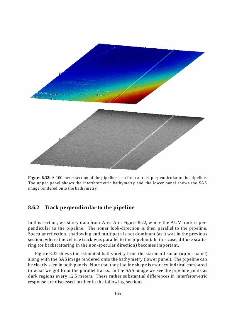
Figure 8.32: A 100 meter section of the pipeline seen from a track perpendicular to the pipeline.The upper panel shows the interferometric bathymetry and the lower panel shows the SASimage rendered onto the bathymetry.

8.6.2 Track perpendicular to the pipeline

In this section, we study data from Area A in Figure 8.22, where the AUV track is per-pendicular to the pipeline. The sonar look-direction is then parallel to the pipeline.Specular reflection, shadowing and multipath is not dominant (as it was in the previoussection, where the vehicle track was parallel to the pipeline). In this case, diffuse scatte-ring (or backscattering in the non-specular direction) becomes important.

Figure 8.32 shows the estimated bathymetry from the starboard sonar (upper panel)along with the SAS image rendered onto the bathymetry (lower panel). The pipeline canbe clearly seen in both panels. Note that the pipeline shape is more cylindrical comparedto what we got from the parallel tracks. In the SAS image we see the pipeline joints asdark regions every 12.5 meters. These rather substantial differences in interferometricresponse are discussed further in the following sections.

165

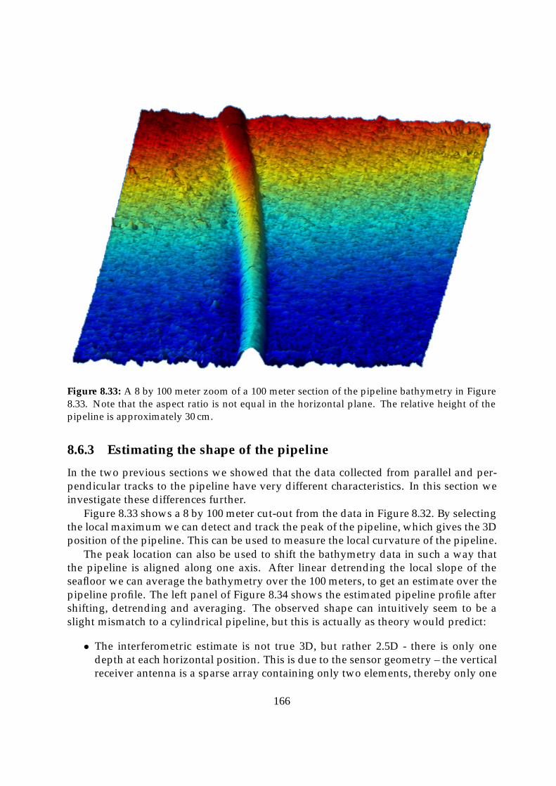
Figure 8.33: A 8 by 100 meter zoom of a 100 meter section of the pipeline bathymetry in Figure8.33. Note that the aspect ratio is not equal in the horizontal plane. The relative height of thepipeline is approximately 30 cm.

8.6.3 Estimating the shape of the pipeline

In the two previous sections we showed that the data collected from parallel and per-pendicular tracks to the pipeline have very different characteristics. In this section weinvestigate these differences further.

Figure 8.33 shows a 8 by 100 meter cut-out from the data in Figure 8.32. By selectingthe local maximum we can detect and track the peak of the pipeline, which gives the 3Dposition of the pipeline. This can be used to measure the local curvature of the pipeline.

The peak location can also be used to shift the bathymetry data in such a way thatthe pipeline is aligned along one axis. After linear detrending the local slope of theseafloor we can average the bathymetry over the 100 meters, to get an estimate over thepipeline profile. The left panel of Figure 8.34 shows the estimated pipeline profile aftershifting, detrending and averaging. The observed shape can intuitively seem to be aslight mismatch to a cylindrical pipeline, but this is actually as theory would predict:

• The interferometric estimate is not true 3D, but rather 2.5D - there is only onedepth at each horizontal position. This is due to the sensor geometry – the verticalreceiver antenna is a sparse array containing only two elements, thereby only one

166

measurement can be done.

• We apply a window of 9 by 9 image-samples to produce one interferometric esti-mate (see Section 8.1). This is done to reduce variance in the depth estimate. Ineffect, the bathymetry is lowpass filtered with an 18 cm window.

The measured height of the pipeline relative to the surrounding in the left panel ofFigure 8.34 is around 30 cm, which fits with the diameter of the pipeline. The burial ofthe pipeline is unknown. We also tried to estimate the diameter based on the curvatureof the profile, but due to the lowpass filtering, the profile is not cylindrical and theestimate varied from 33 to 40 cm depending on where we measured.

We have also performed similar analysis on the SAS image and averaged the inten-sity data to get a profile of the pipeline. The estimated width (and thereby diameter)varied from 30 to 57 cm depending on whether we measured -3 dB or -10 dB from thepeak. This result is somewhat expected as the main lobe width of the imaging system isspecified as 2.5 cm at -3 dB but wider at -10 dB.

In the right panel of Figure 8.34 we see an estimate of the pipeline profile from themerged bathymetry data using the parallel tracks. We have applied the same shiftingand averaging method as described above to produce the profile. The profile showseveral important features: Firstly, it is clear that the profile is dominated by the twospecular reflections. Since the AUV height is different for the two tracks (see Figure8.30) the specular reflections are at different depths. They are also smeared in rangedue to the interferometric window. Secondly, it seems that there is little echo from thetop of the pipeline. There are some energy at the center of the pipeline profile, but theheight is not above the specular reflections. Thirdly, there are energy below the seafloorsurface, which indicates that we receive a multipath bounced onto the seafloor before itis echoed back into the sonar.

8.6.4 Summary

In this section we have shown preliminary results from a pipeline survey using HISASas primary sensor. We have focused on two different sections of the pipeline, one wherethe AUV tracks were parallel to the pipeline on each side and one where the track wasperpendicular to the pipeline.

In the parallel tracks the pipeline is easily identifiable. The backscattered field is af-fected by specular reflection, shadowing and multipath. These features are also presentin the interferometric data, but the estimated bathymetry is still usable to separate thepipeline from the rest of the seafloor. The shadowing can be eliminated by merging thedata from two sides. The bathymetric pipeline profile does not fit a cylindrical shape,as expected, since the interferometric bathymetry estimate is dominated by the specularreflection.

In the track perpendicular to the pipeline, the pipeline is easily distinguished fromthe rest of the seafloor, both in the SAS images and in the interferometric data. Thebathymetric profile of the pipeline looked more like a lowpass filtered cylindrical object.

167

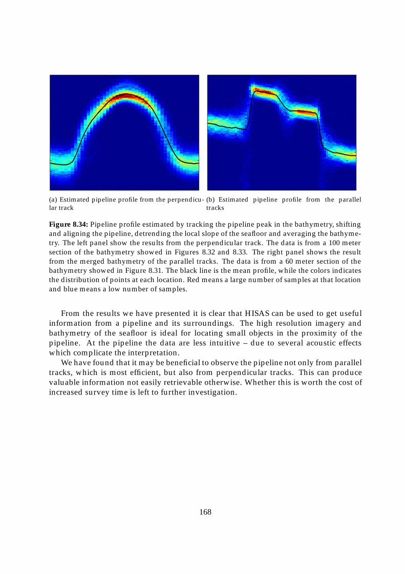
(a) Estimated pipeline profile from the perpendicu-lar track

(b) Estimated pipeline profile from the paralleltracks

Figure 8.34: Pipeline profile estimated by tracking the pipeline peak in the bathymetry, shiftingand aligning the pipeline, detrending the local slope of the seafloor and averaging the bathyme-try. The left panel show the results from the perpendicular track. The data is from a 100 metersection of the bathymetry showed in Figures 8.32 and 8.33. The right panel shows the resultfrom the merged bathymetry of the parallel tracks. The data is from a 60 meter section of thebathymetry showed in Figure 8.31. The black line is the mean profile, while the colors indicatesthe distribution of points at each location. Red means a large number of samples at that locationand blue means a low number of samples.

From the results we have presented it is clear that HISAS can be used to get usefulinformation from a pipeline and its surroundings. The high resolution imagery andbathymetry of the seafloor is ideal for locating small objects in the proximity of thepipeline. At the pipeline the data are less intuitive – due to several acoustic effectswhich complicate the interpretation.

We have found that it may be beneficial to observe the pipeline not only from paralleltracks, which is most efficient, but also from perpendicular tracks. This can producevaluable information not easily retrievable otherwise. Whether this is worth the cost ofincreased survey time is left to further investigation.

168

Chapter 9

Summary and conclusions

In this thesis we have developed methods for robust and accurate interferometric SAS.We have emphasized that a priori depth information is an important prerequisite forSAS imaging and developed a solution through sidescan depth estimation. We havedescribed the integration of depth information into the navigation and the image for-mation. Finally, we have developed a method for interferometric SAS, and performeddetailed studies into possible advances and applications.

One of two main topics in this thesis is a thorough description of the geometry ininterferometric sidelooking sonar. An important conclusion is that the interferometrictime series are not only time delayed relative to each other, but also dilated. We havedeveloped a new mathematical description of the geometry in sidelooking sonar andshown how an approximation-free solution for the depth can be obtained.

The other main topic is time delay estimation. We have argued that a standardtime delay estimator like the cross-correlation function is sub-optimum on interfero-metric time series due to the relative dilation. We presented two solutions: The cross-uncertainty function and a nonlinear co-registration by interpolating the data onto ana priori ground-range. We showed that the cross-uncertainty function has better per-formance than the cross-correlation function on time delayed time series and approxi-mately equal performance on non-dilated time series. We also introduced an improvedcross-correlation based estimator on data with asymmetrical spectra.

We have developed two depth estimation routines: Sidescan bathymetry and SASinterferometry. We introduced a well performing unwrapper for cross-correlation basedsidescan bathymetry estimates, and briefly discussed the concept of iterative SAS inter-ferometry. A short summary on the difference between SAS interferometry and SARinterferometry tried to shed light on where typical SAS-systems are similar to SAR-systems.

There is a lack of a standard on how to measure resolution in bathymetric maps.We suggested flank length as a measure of the horizontal resolution in depth maps. Weestimated the flank length on simulated datasets to verify the theoretical values. Theconclusion was the implemented sidescan bathymetry and SAS interferometry perfor-med very close to the theoretical limits when it comes to horizontal resolution. When

169

it comes to the vertical precision of the depth estimation, it followed the theoreticalperformance within a factor of two. An important observation is that it is the SNR esti-mated from the coherence which limits the vertical precision, not the actual SNR. Thisis because the estimated SNR also includes model errors like baseline decorrelation.

We presented results from a number of studies using experimental HISAS data. Thetopics are to a large extent unrelated. The conclusions are as follow:

• It seems unrealistic to achieve depth estimates with full SAS image resolution.Due to the speckly nature of SAS images, some kind of filtering has to be applied.The phase-difference filter is a maximum likelihood estimate of the interferometricphase-difference. The size of the filter is a trade-off between vertical precisionand horizontal resolution. At some level the precision will not be improved byincreasing the size of the filter, since it assumes homogeneity. A better solution isthen to post-smooth the depth estimates.

• In slant-range sidescan bathymetry (or other cases where the time delay estimateis limited by dilation of the time series) the cross-uncertainty function outperformsa standard cross-correlation based technique with as much as an equivalent 20 dBSNR increase. A cross-uncertainty based technique is therefore a good alterna-tive to the non-linear co-registration in ground-range (which we have used in therest of this thesis). The dilation-factor may also provide useful information whichcannot be obtained from the time delay estimate itself.

• A split-bandwidth technique which divides the bandwidth into sub-bands, canbe used to resolve the 2π ambiguities in SAS interferometry. We implemented asimple technique, which outperformed a standard 2D unwrapping technique (theGoldstein Branch cut algorithm) on large scale. However, due to the simplicity ofthe method it failed on a small number of random pixels.

• The weighted bilateral filter outperforms a large phase-difference filter, a weightedsmoothing filter and a weighted median filter when it comes to smoothing depthmaps, while retaining sharp edges.

• Sidescan bathymetry using HISAS has very similar performance to depth estima-tion using an EM 3000 multibeam echo sounder. For simultaneously operationusing an HUGIN 1000-MR AUV in typical geometry, the EM 3000 has slightly bet-ter resolution while HISAS has larger area coverage rate. HISAS SAS bathymetryhas large area coverage rate and superior resolution. We also found that there is asmall discrepancy remaining between the two sensors.

• A HISAS interferometric SAS can be used to get useful information from a pipelineand its surroundings. We have found that due to acoustic effects which compli-cates the interpretation, it can be beneficial to observe the pipeline not only fromparallel tracks, but also from perpendicular tracks.

170

9.1 Suggested future work

Some of the topics we investigated in this thesis have not been addressed to their fullextent, due to a limited time span. A few of them which deserves further attention, arelisted below:

• An expanded cross-uncertainty estimator which estimates the dilation both fromthe geometry and from the data itself. A goal should be to find a continuousmodel-based estimate of the delay and the dilation instead of the patch-based me-thod presented in this thesis.

• A better and more robust split-bandwidth implementation based on the probabi-lity density functions for each sub-band having the correct wrap interval. Eitherby using a maximum likelihood method by exploiting deterministic contextualinformation consisting in the approximation of the depth surface through localplanes (Budillon et al., 2005) or by fusing the interferograms from each sub-bandwith a coherence weighted Kalman filter (Lanari et al., 1996).

• A study of the discrepancy between HISAS and the EM 3000 when operated si-multaneously on the HUGIN 1000-MR AUV.

• An even more thorough study of the acoustic effects when using sidelooking sonarto survey elevated man-made objects like a pipeline.

171

172

Bibliography

EM 3000, Multibeam echo sounder, rev. C edition, October 2003.

Triton Imaging, Inc. eXtended Triton Format (XTF), rev. 26 edition, December 2008.

Kongsberg EM Series Multibeam echo sounder: EM datagram formats, 850th edition, January2010.

MATLAB 7 MAT-File Format, version 7.11 edition, September 2010.

R. A. Altes. Some invariance properties of the wide-band ambiguity function. J. Acoust. Soc.Am., 53(4): 1154–1160, 1973.

J. T. Ambrose and A. Geneva. Wide swath bathymetric sonar error modeling for a hydrogra-phic survey ship. In OCEANS ’95 MTS/IEEE, pp. 339–346. San Diego, CA, USA, October1995.

R. Bamler and M. Eineder. Accuracy of differential shift estimation by correlation and split-bandwidth interferometry for wideband and delta-k sar systems. IEEE Trans. Geosci. RemoteSensing., 2(2): 151–155, 2005.

R. Bamler and P. Hartl. Synthetic aperture radar interferometry. Inverse problems, 14(4):1–54, 1998.

K. L. Bell, Y. Steinberg, Y. Ephraim and H. L. Van Trees. Extended Ziv-Zakai lower boundfor vector parameter estimation. IEEE Trans. Inform. Theory, 43(2): 624–637, 1997.

A. Bellettini and M. A. Pinto. Theoretical accuracy of synthetic aperture sonar micronaviga-tion using a displaced phase-center antenna. IEEE J. Oceanic Eng., 27(4): 780–789, 2002.

S. Benedetto and E. Biglieri. Principles of digital transmission: With wireless applications.Kluwer Academic/Plenum Publishers, 233 Spring Street, New York, NY 10013, USA,1999.

J. S. Bird and P. Kraeutner. Cramer-Rao bound investigation of swath bathymetry accuracy. InProceedings of Oceans 2001 MTS/IEEE, pp. 1640–1647. Honolulu, HI, USA, November2001.

173

J. S. Bird and G. K. Mullins. Analysis of swath bathymetry sonar accuracy. IEEE J. OceanicEng., 30 (2): 372–390, 2005.

W. W. Bonifant Jr, M. A. Richards and J. H. McClellan. Interferometric height estimationof the seafloor via synthetic aperture sonar in the presence of motion errors. IEE Proc. Radar,Sonar Navig., 147 (6): 322–330, 2000.

L. Brekhovskikh and Y. Lysanov. Fundamentals of ocean acoustics, volume 8 of SpringerSeries in electrophysics. Springer-Verlag, Berlin, Germany, 1982.

A. R. Brenner. Proof of concept for airborne SAR imaging with 5 cm resolution in X-band. InProceedings of EUSAR 2010. Aachen, Germany, June 2010.

A. R. Brenner and L. Roessing. Radar imaging of urban areas by means of very high-resolutionSAR and interferometric SAR. IEEE Trans. Geosci. Remote Sensing., 46(10): 2971–2982,October 2008.

A. R. Brenner, L. Roessing and P. Berens. Potential of very high resolution SAR interferome-try for urban building analysis. In Proceedings of EUSAR 2010. Aachen, Germany, June2010.

D. R. K. Brownrigg. The weighted median filter. In In Communications of the ACM, volume27 (8), pp. 807–818. 1984.

M. P. Bruce. A processing requirement and resolution capability comparison of side-scan andsynthetic-aperture sonars. IEEE J. Oceanic Eng., 17(1): 106–117, 1992.

A. Budillon, G. Ferraiuolo, V. Pascazio and G. Schirinzi. Multichannel SAR interferometryvia classical and Bayesian estimation techniques. Journal on Applied Signal Processing, 20:3180–3193, 2005.

W. S. Burdic. Underwater acoustic system analysis. Prentice-Hall, 113 Sylvan Avenue,Englewood Cliffs, NJ 07632, USA, 1984.

H. J. Callow. Signal processing for synthetic aperture sonar image enhancement. Ph.D. thesis,University of Canterbury, Christchurch, New Zealand, 2003.

H. J. Callow, M. P. Hayes and P. T. Gough. Motion-compensation improvement for widebeam,multiple-receiver SAS systems. IEEE J. Oceanic Eng., 34 (3): 262–268, 2009.

W. G. Carrara, R. S. Goodman and R. M. Majewski. Spotlight synthetic aperture radar:Signal processing algorithms. Artech House, 685 Canton Street, Norwood, MA 02062,USA, 1995.

Y. T. Chan and K. C. Ho. Joint time-scaling and TDOA estimation: Analysis and fast approxi-mation. IEEE Trans. Signal Processing, 53 (8): 2625–2634, 2005.

174

J. C. Curlander and R. N. McDonough. Synthetic aperture radar: Systems and signal pro-cessing. Wiley Series in remote sensing. John Wiley & Sons, 605 Third Avenue, NewYork, NY 10158, USA, 1991.

L. J. Cutrona. Comparison of sonar system performance achievable using synthetic-aperturetechniques with the performance achievable by more conventional means. J. Acoust. Soc. Am.,58 (2): 336–348, August 1975.

P. N. Denbigh. Swath bathymetry: Principles of operation and an analysis of errors. IEEE J.Oceanic Eng., 14 (4): 289–298, 1989.

P. N. Denbigh. Signal processing strategies for a bathymetric sidescan sonar. IEEE J. OceanicEng., 19 (3): 382–390, 1994.

J. V. DiFranco and W. L. Rubin. Radar detection. Artech House, 685 Canton Street, Nor-wood, MA 02062, USA, 1980.

L. B. Dozier, J. S. Hanna and C. R. Pearson. Treatments of incoherent scattering for the para-bolic equation and astral propagation models. In Ocean Variability & Acoustic Propagation,edited by J. Potter and A. Warn-Varnas, pp. 265–281. Kluwer Academic Publishers,Dordrecht, The Netherlands, 1991.

J. H. G. Ender and A. R. Brenner. PAMIR a wideband phased array SAR/MTI system. IEEProc. Radar, Sonar Navig., 150(3): 165–172, 2003.

C. Falsi, D. Dardari, L. Mucchi and M. Z. Win. Time of arrival estimation for uwb localizersin realistic environments. Journal on Applied Signal Processing, 2006: 152–164, 2006.

J. R. Fienup. Phase error correction by shear averaging. In Signal Recovery and synthesis III,pp. 134–137. Optical Society of America, 1989.

S. M. Flatte, R. Dashen, W. H. Munk, K. M. Watson and F. Zachariasen. Sound transmis-sion through a fluctuating ocean. Cambridge monographs on mechanics and appliedmathematics. Cambridge University Press, Trumpington Street, Cambridge CB2 1RP,UK, 1979.

G. Fornaro and G. Franceschetti. Image registration in interferometric SAR processing. IEEProc. Radar, Sonar Navig., 142(6): 313–320, December 1995.

T. G. Fossum, T. O. Sæbø, B. Langli, H. J. Callow and R. E. Hansen. HISAS 1030 - highresolution interferometric synthetic aperture sonar. In Proceedings of the Canadian Hydro-graphic Conference and National Surveyors Conference. Victoria, BC, Canada, May 2008.

G. Franceschetti and R. Lanari. Synthetic aperture radar processing. CRC Press, 2000Corporate Blvd. Boca Raton, FL 33431, USA, 1999.

175

K. Gade. NavLab, a generic simulation and post-processing tool for navigation. EuropeanJournal of Navigation, 2(4): 51–59, November 2004.

F. Gatelli, A. M. Guarnieri, F. Parizzi, P. Pasquali, C. Prati and F. Rocca. The wavenumbershift in SAR interferometry. IEEE Trans. Geosci. Remote Sensing., 32(4): 855–865, July1994.

R. Gauer, A. McFadzean and C. Reid. An automated sidescan sonar pipeline inspectionsystem. In OCEANS ’99 MTS/IEEE, pp. 811–816. Seattle, WA, USA, September 1999.

N. Gebert, G. Krieger and A. Moreira. Multichannel azimuth processing in ScanSAR andTOPS mode operation. IEEE Trans. Geosci. Remote Sensing., 48(7): 2994–3308, July 2010.

D. C. Ghiglia and M. D. Pritt. Two-dimensional phase unwrapping: Theory, algorithms, andsoftware. John Wiley & Sons, 605 Third Avenue, New York, NY 10158, USA, 1998.

I. A. Glover and P. M. Grant. Digital communications. Prentice-Hall Europe, HemelHempstead, Hertfordshire HP2 7EZ, UK, 1998.

R. D. Gonzales and R. E. Woods. Digital image processing. Addison-Wesley PublishingCompany, Reading, MA, USA, 1992.

P. T. Gough and D. W. Hawkins. Imaging algorithms for a strip-map synthetic aperture sonar:Minimizing the effects of aperture errors and aperture undersampling. IEEE J. Oceanic Eng.,22 (1): 27–39, 1997.

H. D. Griffiths, T. A. Rafik, Z. Meng, C. F. N. Cowan, H. Shafeeu and D. K. Anthony.Interferometric synthetic aperture sonar for high-resolution 3-D mapping of the seabed. IEEProc. Radar, Sonar Navig., 144 (2): 96–103, 1997.

J. Groen, R. E. Hansen, H. J. Callow, J. C. Sabel and T. O. Sæbø. Shadow enhancement insynthetic aperture sonar using fixed focusing. IEEE J. Oceanic Eng., 34 (3): 269–284, 2009.

P. E. Hagen and R. E. Hansen. Area coverage rate of synthetic aperture sonars. In Proceedingsof Oceans 2007 Europe. Aberdeen, UK, June 2007.

P. E. Hagen, N. J. Størkersen and K. Vestgard. Hugin – use of uuv technology in marineapplications. In OCEANS ’99 MTS/IEEE, pp. 967–972. Seattle, WA, USA, September1999.

P. E. Hagen, N. Størkersen and K. Vestgard. The HUGIN 1000 military AUV system. InUDT Europa 2004 Conference Proceedings. Nice, France, June 2004.

P. E. Hagen, N. Størkersen and K. Vestgard. HUGIN AUV’s in marine research – today andtomorrow. In Proceedings from International Workshop on Underwater Robotics (IWUR).Genoa, Italy, November 2005.

176

P. E. Hagen, R. E. Hansen and B. Langli. Interferometric synthetic aperture sonar for theHUGIN 1000-MR AUV. In UDT Pacific 2006 Conference Proceedings. San Diego, CA,USA, November 2006.

R. E. Hansen, T. O. Sæbø, H. J. Callow, P. E. Hagen and B. Langli. Synthetic aperture sonarprocessing for the HUGIN AUV. In Proceedings of Oceans 2005 Europe. Brest, France,June 2005.

R. E. Hansen, T. O. Sæbø, H. J. Callow and B. Langli. The SENSOTEK interferometric syn-thetic aperture sonar: Results from HUGIN AUV trials. In Proceedings of the 8th EuropeanConference on Underwater Acoustics. Carvoeiro, Portugal, June 2006.

R. E. Hansen, H. J. Callow and T. O. Sæbø. The effect of sound velocity variations on syntheticaperture sonar. In Proceedings of Underwater Acoustic Measurements 2007. Crete, Greece,June 2007.

R. E. Hansen, H. J. Callow, T. O. Sæbø, S. A. Synnes, P. E. Hagen, T. G. Fossum andB. Langli. Synthetic aperture sonar in challenging environments: Results from the HISAS1030. In Proceedings of Underwater Acoustic Measurements 2009. Nafplion, Greece, June2009. CDROM (ISBN 978-960-98883-4-9).

R. E. Hansen, H. J. Callow, T. O. Sæbø and S. A. V. Synnes. Challenges in seafloor imagingand mapping with synthetic aperture sonar. In Proceedings of the Eighth European conferenceon synthetic aperture radar. Aachen, Germany, June 2010a. CDROM (ISBN 978-3-8007-3272-2).

R. E. Hansen, T. O. Sæbø, H. J. Callow and P. E. Hagen. Interferometric synthetic aper-ture sonar in pipeline inspection. In Proceedings of OCEANS 2010 MTS/IEEE. Sydney,Australia, May 2010b. CDROM (ISBN 978-1-4244-5222-4).

A. Hanssen, J. Kongsli, R. E. Hansen and S. Chapman. Statistics of synthetic aperture sonarimages. In Proceedings of Oceans 2003 MTS/IEEE, pp. 2635–2640. San Diego, CA, USA,September 2003.

R. F. Hanssen. Radar interferometry: Data interpretation and error analysis. Kluwer Acade-mic Publishers, P. O. Box 17, 3300 AA Dordrecht, The Netherlands, 2001.

F. J. Harris. On the use of windows for harmonic analysis with the discrete fourier tranform.Proceedings of the IEEE, 66 (1): 51–83, 1978.

D. W. Hawkins. Synthetic aperture imaging algorithms: With application to wideband sonar.Ph.D. thesis, University of Canterbury, Christchurch, New Zealand, 1996.

M. P. Hayes and P. T. Gough. Synthetic aperture sonar: A review of current status. IEEE J.Oceanic Eng., 34 (3): 207–224, 2009.

177

Ø. Hegrenæs, T. O. Sæbø, P. E. Hagen and B. Jalving. Horizontal mapping accuracy inhydrographic AUV surveys. In Proceedings of the IEEE Autonomous Underwater Vehicles2010. Monterey, CA, USA, September 2010.

S. Holm. Optimum FFT-based frequency acquisition with application to COSPAS-SARSAT.IEEE Trans. Aerospace and Electronic Systems., 29 (2): 464–475, 1993.

S.-H. Hong, H.-S. Jung and J.-S. Won. Extraction of ground control points (GCPs) fromsynthetic aperture radar images and SRTM DEM. International Journal of Remote Sensing,27(18): 3813–3829, 2006.

D. R. Jackson and M. D. Richardson. High-frequency seafloor acoustics. Springer Mono-graph series in underwater acoustics. Springer Science+Business Media, 233 SpringStreet, New York, NY 10013, USA, 2007.

J. C. V. Jakowatz, D. E. Wahl, P. H. Eichel, D. C. Ghiglia and P. A. Thompson. Spotlight-mode synthetic aperture radar: A signal processing approach. Kluwer Academic Publi-shers, P. O. Box 17, 3300 AA Dordrecht, The Netherlands, 1996.

B. Jalving, K. Gade, O. K. Hagen and K. Vestgard. A toolbox of aiding techniques for the HU-GIN AUV integrated inertial navigation system. In Proceedings of Oceans 2003 MTS/IEEE,pp. 1146–1153. San Diego, CA, USA, September 2003.

D. H. Johnson and D. E. Dudgeon. Array signal processing: Concepts and techniques. Si-gnal processing series. Prentice Hall, 113 Sylvan Avenue, Englewood Cliffs, NJ 07632,USA, 1993.

C. D. de Jong, G. Lachapelle, A. Skone and I. A. Elema. Hydrography. Series on Ma-thematical geodesy and positioning. VSSD, Leeghwaterstraat 42, 2628 CA Delft, TheNetherlands, 2002.

L. R. Joughin and D. P. Winebrenner. Effective number of looks for a multilook interferometricphase distribution. In Proceedings of Geoscience and Remote Sensing Symposium (IGARSS)1994, pp. 2276–2278. Pasadena, CA, USA, August 1994.

D. Just and R. Bamler. Phase statistics of interferograms with applications to synthetic apertureradar. Appl. Opt., 33(20): 4361–4368, 1994.

S. M. Kay. Fundamentals of statistical signal processing. Estimation theory. Prentice Hall,113 Sylvan Avenue, Englewood Cliffs, NJ 07632, USA, 1993.

D. Kincaid and W. Cheney. Numerical analysis. Brooks/Cole Publishing Company, 511Forest Lodge Road, Pacific Grove, CA 93950, USA, second edition, 1991.

B. Kjellesvig. Improved height estimation algorithms for synthetic aperture sonar interferome-try. Master’s thesis, University of Oslo, Oslo, Norway, 2006.

178

C. K. Knapp and G. C. Carter. The generalized correlation method for estimation of time delay.IEEE Trans. Acoust., Speech, Signal Processing, ASSP-24(4): 320–327, 1976.

G. Krieger, A. Moreira, H. Fiedler, I. Hajnsek, M. Werner, M. Younis and M. Zink.TanDEM-X: A satellite formation for high-resolution SAR interferometry. IEEE Trans.Geosci. Remote Sensing., 45(11): 3317–3341, November 2007.

G. Krieger, I. Hajnsek, K. P. Papathanassiou, M. Younis and A. Moreira. Interferome-tric synthetic aperture radar (SAR) missions employing formation flying. Proceedings of theIEEE, 98(5): 816–843, May 2010.

R. Lanari, G. Fornaro, D. Riccio, M. Migliaccio, K. P. Papathanassiou, J. R. Moreira,M. Schwabisch, L. Dutra, G. Puglisi, G. Franceschetti and M. Coltelli. Generation ofdigital elevation models by using SIR-C/X-SAR multifrequency two-pass interferometry: TheEtna case study. IEEE Trans. Geosci. Remote Sensing., 34(5): 1097–1114, 1996.

M. Lange and P. Gill. An airborne interferometric SAR system for high performance 3D map-ping. In Proc. of SPIE Radar Sensor Technology XIII, volume 7308. Orlando, FL, USA,April 2009.

N. Levanon. Radar principles. John Wiley & Sons, 605 Third Avenue, New York, NY10158, USA, 1988.

G. Llort-Pujol, C. Sintes and X. Lurton. A new approach for fast and high-resolution interfe-rometric bathymetry. In Proceedings of Oceans 2006 Asia Pacific. Singapore, May 2006.

X. Lurton. Swath bathymetry using phase difference: Theoretical analysis of acoustical measu-rement precision. IEEE J. Oceanic Eng., 25 (3): 351–363, 2000.

X. Lurton. An introduction to underwater acoustics: Principles and applications. SpringerPraxis Publishing, Chichester, UK, 2002.

A. P. Lyons and D. A. Abraham. Statistical characterization of high-frequency shallow-waterseafloor backscatter. J. Acoust. Soc. Am., 106 (3): 1307–1315, 1999.

S. N. Madsen, H. A. Zebker and J. Martin. Topographic mapping using radar interferometry:Processing techniques. IEEE Trans. Geosci. Remote Sensing., 31(1): 246–256, 1993.

J. H. McClellan, R. W. Schafer and M. A. Yoder. Signal processing first. Prentice Hall,Upper Saddle River, NJ 07458, USA, 2003.

Ø. Midtgaard, T. O. Sæbø and H. J. Callow. Automated recognition of short-tethered objectswith interferometric synthetic aperture sonar. In Proceedings of Oceans 2007 MTS/IEEE.Vancouver, Canada, October 2007.

Ø. Midtgaard, T. O. Sæbø and R. E. Hansen. Estimation of target detection/classificationperformance using interferometric sonar coherence. In Proceedings of Underwater AcousticMeasurements 2009. Nafplion, Greece, June 2009. CDROM (ISBN 978-960-98883-4-9).

179

S. K. Mitra. Digital signal processing: A computer based approach. McGraw-Hill, 1221Avenue of the Americas, New York, NY 10020, USA, 2002.

R. Moddemeijer. On the determination of the position of extrema of sampled correlators. IEEETrans. Signal Processing, 39 (1): 216–219, 1991.

C. de Moustier, P. F. Lonsdale and A. N. Shor. Simultaneous operation of the Sea Beammultibeam echo-sounder and the SeaMARC II bathymetric sidescan sonar system. IEEE J.Oceanic Eng., 15(2): 84–94, 1990.

J. A. Ogilvy. Theory of wave scattering from random rough surfaces. Institute of PhysicsPublishing, Redcliffe Way, Bristol BSI 6NX, UK, 1991.

C. Oliver and S. Quegan. Understanding synthetic aperture radar images. SciTech Publi-shing, Raleigh, NC 27613, USA, 2004.

P. Z. Peebles. Probability, random variables and random signal principles. McGraw-Hill se-ries in electrical and computer engineering. McGraw-Hill, 1221 Avenue of the Ame-ricas, New York, NY 10020, USA, fourth edition, 2001.

Y. Petillot, S. Reed and J. Bell. Real time AUV pipeline detection and tracking using side scansonar and multi-beam echosounder. In OCEANS ’02 MTS/IEEE, pp. 217–222. Biloxi, MS,USA, October 2002.

M. Pinto. 2003. Private communication.

M. A. Pinto. High resolution seafloor imaging with synthetic aperture sonar. IEEE OceanicEng. Newsletter, pp. 15–20, Summer 2002.

A. H. Quazi. An overview on the time delay estimate in active and passive systems for targetlocalization. IEEE Trans. Acoust., Speech, Signal Processing, ASSP-29(3): 527–533, 1981.

B. Rabus, M. Eineder, A. Roth and R. Bamler. The shuttle radar topography mission – anew class of digital elevation models acquired by spaceborne radar. Photogramm. Rem. Sens.,57(4): 241–262, 2003.

S. Reed, Y. Petillot and J. Bell. Automated approach to classification of mine-like objects insidescan sonar using highlight and shadow information. IEE Proc. Radar, Sonar Navig., 151:48–56, 2004.

M. A. Richards. Fundamentals of radar signal processing. The McGraw Hill Companies,Two Penn Plaza, New York, NY 10121, USA, 2005.

D. W. Ricker. Echo signal processing. Kluwer Academic Publishers, P. O. Box 17, 3300 AADordrecht, The Netherlands, 2003.

E. Rodriguez and J. M. Martin. Theory and design of interferometric synthetic aperture radars.Radar and Signal Processing, IEE Proceedings F, 139 (2): 147–159, 1992.

180

K. D. Rolt and H. Schmidt. Effects of refraction on synthetic aperture sonar imaging. J.Acoust. Soc. Am., 95(6): 3424–3429, 1994.

P. A. Rosen, S. Hensley, I. R. Joughin, F. K. Li, S. N. Madsen, E. Rodriguez and R. M.Goldstein. Synthetic aperture radar interferometry. Proceedings of the IEEE, 88(3): 333–382, 2000.

K. Rottmann. Matematisk formelsamling. Bracan Forlag, Nørhaven, Denmark, third edi-tion, 1995. In Norwegian.

T. O. Sæbø and R. E. Hansen. A comparison between interferometric SAS and interferometricSAR. In Proceedings of the Institute of Acoustics. Lerici, Italy, September 2010.

T. O. Sæbø and B. Langli. Comparison of EM 3000 multibeam echo sounder and HISAS 1030interferometric synthetic aperture sonar for seafloor mapping. In Proceedings of ECUA 2004,pp. 451–461. Istanbul, Turkey, July 2010.

T. O. Sæbø, R. E. Hansen, H. J. Callow and B. Kjellesvig. Using the cross-ambiguity functionfor improving sidelooking sonar height estimation. In Proceedings of Underwater AcousticMeasurements 2007, pp. 309–316. Crete, Greece, June 2007a.

T. O. Sæbø, R. E. Hansen and A. Hanssen. Relative height estimation by cross-correlatingground-range synthetic aperture sonar images. IEEE J. Oceanic Eng., 32(4): 971–982, Octo-ber 2007b.

T. O. Sæbø, B. Langli, H. J. Callow, E. O. Hammerstad and R. E. Hansen. Bathymetriccapabilities of the HISAS interferometric synthetic aperture sonar. In Proceedings of Oceans2007 MTS/IEEE. Vancouver, Canada, October 2007c.

T. O. Sæbø, R. E. Hansen and Ø. Midtgaard. Filtering of high resolution interferometric syn-thetic aperture sonar. In Proceedings of Underwater Acoustic Measurements 2009. Nafplion,Greece, June 2009. CDROM (ISBN 978-960-98883-4-9).

T. O. Sæbø, H. J. Callow and P. E. Hagen. Pipeline inspection with synthetic aperture sonar.In Proceedings of the 33th Scandinavian Symposium on Physical Acoustics. Geilo, Norway,February 2010. Online (http://www.iet.ntnu.no/en/groups/akustikk/meetings/SSPA/2010).

R. Shiavi. Introduction to Applied Statistical Signal Analysis. Academic Press, 525 B. St.Suite 1900, San Diego, CA 92101, USA, 1999.

G. Shippey, P. Ulriksen and Q. Liu. Wideband swath bathymetry, SAS autofocus and under-water navigation fixes: Three related problems in echo/image correlation. In IAC/IEE SonarSignal Processing Conference, pp. 483–491. Weymouth, UK, December 1998.

M. Soumekh. Fourier array imaging. Prentice Hall, 113 Sylvan Avenue, Englewood Cliffs,NJ 07632, USA, 1994.

181

M. Soumekh. Synthetic aperture radar signal processing. John Wiley & Sons, 605 ThirdAvenue, New York, NY 10158, USA, 1999.

M. Stangl, R. Werninghaus, B. Schweizer, C. Fischer, M. Brandfass, J. Mittermayer andH. Breit. TerraSAR-X technologies and first results. IEE Proc. Radar, Sonar Navig., 153(2):86–95, April 2006.

S. Suchandt, M. Eineder, H. Breit and H. Runge. Analysis of ground moving objects usingSRTM/X-SAR data. Photogramm. Rem. Sens., 61(3-4): 209–224, 2006.

S. A. Synnes. SAS multipath analysis. FFI/RAPPORT To be published, Norwegian De-fence Research Establishment, 2008.

S. A. Synnes, R. E. Hansen and T. O. Sæbø. Assessment of shallow water performance usinginterferometric sonar coherence. In Proceedings of Underwater Acoustic Measurements 2009.Nafplion, Greece, June 2009. CDROM (ISBN 978-960-98883-4-9).

S. A. V. Synnes, H. J. Callow, T. O. Sæbø and R. E. Hansen. Multipass coherent processingon synthetic aperture sonar data. In Proceedings of European Conference on UnderwaterAcoustic (ECUA) 2010. Istanbul, Turkey, July 2010.

J. D. Taylor. Introduction to ultra-wideband radar systems. CRC Press, 2000 Corporate Blvd.Boca Raton, FL 33431, USA, 1994.

C. Tomasi and R. Manduchi. Bilateral filtering for gray and color images. In In Proceedingsof the IEEE International Conference on Computer Vision, pp. 839–846. 1998.

R. Touzi and A. Lopes. Statistics of the stokes parameters and of the complex coherence para-meters in one-look and multilook speckle fields. IEEE Trans. Geosci. Remote Sensing., 34(2):519–531, 1996.

R. Touzi, A. Lopes, J. Bruniquel and P. W. Vachon. Coherence estimation for SAR imagery.IEEE Trans. Geosci. Remote Sensing., 37(1): 135–149, 1999.

R. J. Urick. Principles of underwater sound. Mcgraw-Hill Book Company, Los Altos, CA,USA, third edition, 1983.

H. L. Van Trees. Optimum array processing. Part IV of detection, estimation, and modulationtheory. John Wiley & Sons, 605 Third Avenue, New York, NY 10158, USA, 2002.

L. Wang, A. Bellettini, R. Hollett, A. Tesei, M. Pinto, S. Chapman and K. Gade. InSAS’00:Interferometric SAS and INS aided SAS imaging. In Proceedings of Oceans 2001 MTS/IEEE,pp. 179–187. Honolulu, HI, USA, November 2001.

M. Wei and T. Coyne. Integrated airborne IFSAR mapping system. In Proceedings of XXthISPRS. Beijing, China, July 2008.

182

W. Xu, C. Chang, L. K. Kwoh, H. Lim and W. C. A. Heng. Phase-unwrapping of SARinterferogram with multi-frequency or multi-baseline. In Proceedings of the IEEE 1994 In-ternational Geoscience and Remote Sensing Symposium (IGARSS), pp. 730–732. Istanbul,Turkey, July 1994.

H. A. Zebker and J. Villasenor. Decorrelation in interferometric radar echoes. IEEE Trans.Geosci. Remote Sensing., 30(5): 950–959, 1992.

L. J. Ziomek. Underwater acoustics: A linear systems theory approach. Academic Press,24-28 Oval Road, London NW1 7DX, UK, 1985.

J. Ziv and M. Zakai. Some lower bounds on signal parameter estimation. IEEE Trans. Inform.Theory, IT-15(3): 386–391, 1969.

183

184

About the author — Torstein Olsmo Sæbø was born in 1977 in Bergen, Norway wherehe grew up. He received the cand.mag. (B.E.) degree in physics in 2000 and the cand.scient. (M.Sc.) degree in astrophysics in 2002, from the University of Oslo, Oslo, Nor-way. Since 2002, he has been working as a Scientist at the Maritime Systems Divisionat the Norwegian Defence Research Establishment (FFI), Kjeller, Norway, specializingin the field of synthetic aperture sonar. In 2004 he started to pursuit a Ph.D. degreein the field of synthetic aperture sonar interferometry at the University of Tromsø, De-partment of Physics and Technology. In November 2010, he defended the current Ph.D.thesis, entitled “Seafloor Depth Estimation by means of Interferometric Synthetic Aper-ture Sonar”. The topic reflects his research interest, which are in the areas of signalprocessing, synthetic aperture beamforming and interferometry.