Sea Level Rise Projections for Failaka Island in The State ...

236 Jasem A. Albanai: Sea Level Rise Projections for Failaka Island in The State of Kuwait

Remote Sensing and GIS Analyst, Kuwait City, Kuwait

e-mail: [email protected]

As a result of climate change, many lands are under risk due to the rising sea levels (RSL). Studies show that the mean sea level will likely rise by 0.16 to 0.63 metres before 2050, and 0.2 to 2.5 metres by 2100. Lower-lying islands are more endangered from RSL. One of such islands is Failaka, a small island in Kuwait lying at the entrance of Kuwait Bay, which is located on the north-western side of the Arabian Gulf (Also called the Persian Gulf ). Most of Failaka Island is lower than three meters. The Governmental plans are to develop and populate the island. SLR should be considered in such planning. This study focuses particularly on detecting the areas of Failaka Island which are under high threat from the SLR. To detect these areas, spatial analysis of the Digital elevation model (DEM) are used. DEM is estimated for three SLR scenarios (1, 2 and 3 metres). It is expected that 31% of the island will be under sea level height for the SLR of 1 m; 54% for the SLR of 2 metres; and 87% for the SLR of 3 m. Coastal Vulnerability Index (CVI) is estimated as well. The CVI shows that the eastern coast is the most susceptible with regard to the SLR. The model was validated through using ground elevation points (n = 40), and a positive correlation was found with r^2 of 0.8019. Geographic Information System (GIS) and Remote sensing (RS) are confirmed to be effective tools for estimating spatial influence of the SLR.

Sea Level Rise Projections for Failaka Island in The State of Kuwait Jasem A. Albanai

KEY WORDS ~ Sea level rise ~ Failaka island ~ Kuwait ~ Geographic information system ~ Remote sensing ~ Coastal vulnerability index

1. INTRODUCTION

Scientists continue to confirm that the global sea level change is entirely related to climate change. The increased temperatures on the planet surface lead to thermal expansion in ocean waters, which further contributes to the rise in global sea levels (Titus, 1990). Furthermore, as increasing temperatures on the planet's surface dissolve the giant ice sheets in Greenland and Antarctica, this leading to the global SLR (Englander, 2015).

The SLR during the 20th century was estimated to be 20-25mm (J. A. Church et al., 2013; J. A. Church and White, 2011; Titus, 1990). Global SLR ranged between 0.3 and 3.2 mm per year (J. A. Church and White, 2006; 2011), to about 0.4 to 3.2mm per year (J. A. Church and White, 2011) (Figure 1). It is also worth noting that SLR varies spatially. For example, SLR in the Chesapeake Bay was 3.2mm per year during the last century (Stevenson et al., 2002). In the southern Netherlands, SLR was estimated at 1.7 - 2.7 m between 1940 and 2002 (Becker et al., 2009). The spatial variations in sea level changes are due to multiple natural factors (Nicholls and Mimura, 1998). The Arabian Gulf was exposed to sea level change during the geological timescale (Albanai, 2017). Studies estimate that the current flooding of the Arabian Gulf basin started 10,000 – 15,000 years ago (Holocene) (El-Enin, 1989). In the north-western part on the Arabian Gulf, Alothman, Bos, Fernandes, and Ayhan (2014) have estimated that the absolute sea level rise is 0.8-1.5 mm/year using all the available tide gauge data during 29 years study (1979 – 2007). The results are consistent with global SLR estimate of 0.1-1.9 mm/year (J. A. Church and White, 2011) for the same studied period.

SLR projections for the 21st century vary hugely. Overall, sea level is expected to rise from 0.16 to 0.63m by 2050, and from 0.2 to 2.5m by 2100 (Sweet et al., 2018). Englander (2015) pointed out that SLR is strongly dependant on the rate at which polar ice melts. It is expected that continuous SLR over the 21st century will cause many problems, such as population displacements,

This work is licensed under

doi: 10.7225/toms.v09.n02.008

TRANSACTIONS ON MARITIME SCIENCE 237Trans. marit. sci. 2020; 02: 236-247

Figure 1.Nine different time projections of SLR at the end of this century, ranging from 0.2 to 2.1 m. The IPCC AR4 projection for 2007 does not include accelerated melting rates in Greenland and Antarctica (Englander, 2015; Rahmstorf, 2010; Moore, 2019).

the destruction of coastal infrastructure and coastal erosion. It should be noted that about 10% of the world's population lives within 10 kilometres from the coast (McGranahan, Balk, and Anderson, 2007; United Nations, 2017) and around 40% of the world's population lives within 100 Km of the coast (United Nations, 2017).

DEMs are often used in GIS and are the most common basis for digitally produced relief maps. There are two freely available DEMs for the area of this study: The Shuttle Radar Topography Mission (SRTM) and the Thermal Emission and Reflection Radiometer (ASTER). Both have a spatial resolution of around 30 m^2. Aster DEM is made from satellite stereo images while SRTM is made from RADAR data. Generally, there are three basic sources for the DEMs: (i) data from the topographic maps, which can be digitised; (ii) in-situ data collected with GPS; or (iii) aerial photographs or satellite images (Elkhrachy, 2017).

The integration of GIS and RS offers the possibility of calculating areas of land that may be flooded using DEMs, such as Malik and Abdalla's (2016) and Aleem and Aina's (2013) studies. However, CVI is widely used for spatial modelling of SLR. CVI was applied early by Gornitz et al. (1994). This indicator is calculated by introducing several variables that are believed to affect coastal zones in the event of SLR. Geo-technologies provide an approach to calculate and map this index (Reyes and Blanco, 2012). The variables calculated in CVI are divided into two groups: (i) a set of several physical variables such as slope, coastal erosion, elevations, geomorphology and hydrodynamics (Palmer et al., 2011; Shaw et al., 1998), (ii) human related variables, such as population affected, land use and transportation (Reyes and Blanco, 2012). CVI scores are classified usually into low, moderate and high, based on quantitative and qualitative analysis.

DEMs have horizontal and vertical accuracy. Statistical methods are needed to assess their accuracy. High-resolution DEMs are also subject to assessments of their accuracy (Cooper et al., 2013). Ground elevation points are used to validate DEMs. They could be taken from many sources, such as satellite images, aerial photography, topographic maps or field surveys. The coefficient of determination (r^2) and the Root Mean Square Error (RMSE) are widely used to validate spatial models (Aleem and Aina, 2013). Regression analysis could also be used to build a new empirical DEMs (Alimonte and Zibordi, 2003).

For SLR studies, Cooper et al., (2013) introduced a methodology for studying SLR using LIDAR data. Their study shows the importance of highly accurate data to support decisions. Kumar (2015) modelled future prospects for sea level rise in the Orissa region of India. He worked on the production of a high-resolution digital height model and analysed the model to visualize the impact of sea level rise. Malik and Abdalla (2016) modelled the expected losses of sea level rise on British Columbia. GIS was used to conceptualize the projections in different scenarios, ranging from one to three meters’ rise in sea levels. At the regional level of the study area, Falour et al. (2013) modelled the vulnerability of the Syrian coasts to sea level rise and coastal hazards through GIS and remote sensing. CVI was computed to assess the coastal risk and several factors were taken to compute it, such as geomorphology, topography, coastal curvature, coastal erosion, sea level rise and hydrodynamics, as well as coastal erosion. Al-Jeneid et al. (2008) studied coastal hazards on the Bahrain Kingdom. The study found that 17% of the total area of the country may become below the main sea level if the sea level were to rise 1.5 meters.


Figure 2.The location of Failaka island in the State of Kuwait. The dark areas on Failaka Island represent the sabkhas.

Figure 3.3D model shows Failaka Island elevations (SRTM DEM).

In Kuwait, Alsahli and AlHasem (2016) studied the SLR impact on the Kuwaiti coasts, and the CVI was used to determine the impact of sea level rise, based on ground elevation points from a topographic map, and ASTER GDEM. The study showed that the northern coasts are likely to be the most affected by the sea level rise, while the southern coasts of Kuwait Bay (Doha) and Shuaibah port on the Southern coast are also affected. Another study by Neelamani and Al-Shatti (2014) discussed the sensitivity of the Kuwaiti coasts. The authors used a global model to show the SLR threats along Kuwait coasts. The study showed the rise effect on Bubyian Island, Failaka Island, Kuwait Bay and some Southern coasts. The current study aims to detect the areas of Failaka Island which are under threat from SLR through spatial analysis of DEM and CVI using six physical parameters (elevation, slope, geomorphology, maximum tidal height, maximum wave height and coastal erosion).

1.1. Study Area

Kuwait is a small country, lying on the north-western side of the Arabian Gulf. It is located between latitudes 28° 30’ and 30° 05’ North, and longitudes 47° 30’ and 48° 36’ East (Figure 2). There are nine islands in Kuwait, with Failaka Island the second in size. The total Kuwaiti land area is 17800 Km^2. Kuwait’s coastline is more than 700 Km including the islands’ maritime borders and new human-made coasts. The State of Kuwait has a desert climate and is affected by the tropical high-pressure region. Kuwait is considered to be a flat land. The surface geomorphology of the State of Kuwait reflects two important factors that govern it: the fluvial deposition in the delta environment and the historical deposition (El-Baz, and Al-Sarawi, 2000).

Failaka Island is located at the entrance of Kuwait Bay, and is at a distance of 20 Km from the coast. It has a total area of 46 Km^2, and coastline of approximately 38 Km. The island was inhabited up to the Gulf War in the 1990 (3500 citizens) with small urban area. The citizens left the island during the war due to the widespread destruction. There are currently two ports on the island, both lying in front of Kuwait City; with one of them working at the moment. Failaka is considered to be a flat land with a few small hills (Figure 3). The highest areas on Failaka reach 9 m above the mean sea level; these are located at the west and south-western parts of the island. Most of the island lands are lower than 2 m above mean sea level. The lower areas are mostly found in the Sabkha regions (Figure 2.). The Failaka coastal zone is affected by two forces: natural and anthropogenic. The tides and waves are the main natural forces controlling the coastal zone. The anthropogenic forces, meanwhile, can be seen clearly in the urban area and beaches. There are 16 different geomorphologic features which can be seen on the island, most important of which are Sabkha, wetland, sandy beach and hard rocks (Al-Sarawi, Marmoush, Lo, and Al-Salem, 1996). The Kuwaiti

Government plans to develop and re-populate the island to achieve the Kuwait master plan 2035 (NewKuwait, 2018).


2. MATERIAL AND METHODS

2.1. Data Description

For mapping the shoreline, the study used satellite imaginary as the main source of data. Landsat 8 image, taken during high tide (10 - 11 AM GMT +3) on 25 August 2014, was used. The image was downloaded from the United States Geological Survey site (2018). To add more accuracy, high-resolution basemap images from the ArcGIS Online (2018), and Google Earth high-resolution database (2018) were used as a reference to validate and edit the shoreline.

Two sources were used to extract the elevations and validate the accuracy: (i) DEM layer from The Shuttle Radar Topography Mission (SRTM) done in 2000 and downloaded from the USGS site (2018). (ii) ground elevation points (n = 40) taken by GPS measurements on September 2018. The DEW was used to compute the SLR scenarios and the ground elevation points were used to validate the accuracy of the model.

The CVI map was prepared using six physical parameters: elevation, slope, geomorphology, maximum tidal height, maximum wave height and coastal erosion. The elevation and slope layers were extracted from the same DEM SRTM layer used to compute the SLR scenarios (USGS, 2018), while the geomorphologic, maximum tidal height and maximum wave height data were taken from Al-Sarawi et al.'s (1996) study of Failaka. The coastal erosion data of the island was obtained from Al-Mutari's (2017).

2.2. Shoreline Mapping

For mapping the shoreline, the Image was calibrated radiometrically using ENVI 5.2 software. The radiometric calibration process changes the pixel values from the digital numbers to radiances. This process helps in detecting the spectral signature of the land cover, which is necessary to class and

analyse the Earth’s features (Elrawy, 2015). Then, pan sharping technique has been applied using ArcGIS 10.4. The multispectral band of Landsat 8 has a low spatial resolution equal to 30 m2, while the panchromatic band has 15 m2 as a spatial resolution. The pan-sharping technique allows us to merge the two bands to benefit from the high spatial resolution of the panchromatic band and the high spectral resolution of the multispectral band. Moreover, a spectral index (band rationing) called the Normalized Difference Water Index was applied on the merged band of Landsat 8 using the band math tool on ENVI software. Several studies have used the spectral indices to map the shoreline and the most important indicator used for this purpose is the NDWI (McFeeters, 2013; Rokni et al., 2014; Al-Mutari, 2017). The NDWI is a related index to water stress and differences. It is calculated as the ratio between the refracted radiations of the near-infrared (NIR) and the short-wave infrared (SWIR) bands. Using more than one band increases the accuracy of shoreline mapping (Ryu et al., 2002). The band rationing method separates the land from the water in two clear colours in contrast to the natural colour, which is often show more gradual changes (Figure 4). The NDWI was applied to delineate the shoreline of Failaka Island using the following equation:

NDWI =( bandG- bandNIR )

( bandG+ bandNIR )(1)

Where G refers to the green band at 0.53 – 0.59 wavelength (μm) and NIR refers to the Near-Infrared band at 0.85 – 0.83 wavelength (μm) of Landsat 8.

After applying the NDWI, shoreline has been edited and validated manually. The manual mapping of shoreline shows good results (Ford, 2013; Meyer et al., 2016). The shoreline has been edited using the satellite basemap data on ArcGIS and Google

Figure 4 .Using NDWI to separate the land from the water and delineate the shoreline.


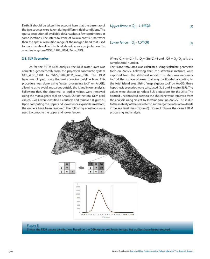
Figure 5.Shows the DEM values distribution. Based on the DEM upper and lower fences, the outliers have been removed.

Earth. It should be taken into account here that the basemap of the two sources were taken during different tidal conditions. The spatial resolution of available data reaches a few centimetres at some locations. The intertidal zone of Failaka coasts is narrower than the spatial resolution range of the merged band that used to map the shoreline. The final shoreline was projected on the coordinate system WGS_1984_UTM_Zone_39N.

2.3. SLR Scenarios

As for the SRTM DEM analysis, the DEM raster layer was corrected geometrically from the projected coordinate system GCS_WGC_1984 to WGS_1984_UTM_Zone_39N. The DEM layer was clipped using the final shoreline polyline layer. This procedure was done using “raster processing tool” on ArcGIS, allowing us to avoid any values outside the island in our analysis. Following that, the abnormal or outlier values were removed using the map algebra tool on ArcGIS. Out of the total DEM pixel values, 0.28% were classified as outliers and removed (Figure 5). Upon computing the upper and lower fences (quartiles method), the outliers have been removed. The following equations were used to compute the upper and lower fences:

Upper fence = Q3 + 1.5*IQR

Lower fence = Q1 - 1.5*IQR

(2)

(3)

Where Q1 = (n+2) ∕ 4 , Q3 = (3n+2) ∕ 4 and IQR = Q3- Q1. n is the samples total number.The island total area was calculated using “calculate geometric tool” on ArcGIS. Following that, the statistical matrices were exported from the statistical report. This step was necessary to find the surface of areas that may be flooded according to the total island area. Using “map algebra tool” on ArcGIS, three hypothesis scenarios were calculated (1, 2 and 3 metre SLR). The values were chosen to reflect SLR projections for the 21st. The flooded unconnected areas to the shoreline were removed from the analysis using “select by location tool” on ArcGIS. This is due to the inability of the seawater to submerge the interior lowlands if the sea level rises (Figure 6). Figure 7. Shows the overall DEM processing and analysis.


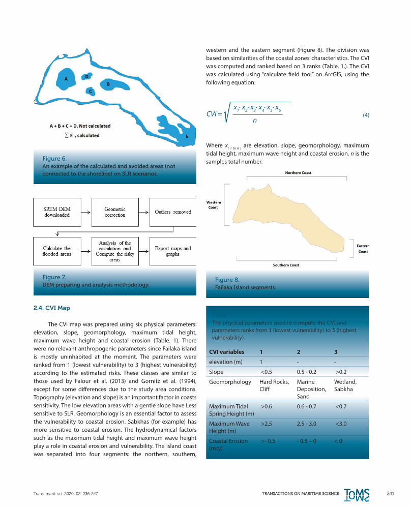
Table 1.The physical parameters used to compute the CVI and parameters ranks from 1 (lowest vulnerability) to 3 (highest vulnerability).

Figure 6.An example of the calculated and avoided areas (not connected to the shoreline) on SLR scenarios.

Figure 7.DEM preparing and analysis methodology.

Figure 8.Failaka Island segments.

2.4. CVI Map

The CVI map was prepared using six physical parameters: elevation, slope, geomorphology, maximum tidal height, maximum wave height and coastal erosion (Table. 1). There were no relevant anthropogenic parameters since Failaka island is mostly uninhabited at the moment. The parameters were ranked from 1 (lowest vulnerability) to 3 (highest vulnerability) according to the estimated risks. These classes are similar to those used by Falour et al. (2013) and Gornitz et al. (1994), except for some differences due to the study area conditions. Topography (elevation and slope) is an important factor in coasts sensitivity. The low elevation areas with a gentle slope have Less sensitive to SLR. Geomorphology is an essential factor to assess the vulnerability to coastal erosion. Sabkhas (for example) has more sensitive to coastal erosion. The hydrodynamical factors such as the maximum tidal height and maximum wave height play a role in coastal erosion and vulnerability. The island coast was separated into four segments: the northern, southern,

western and the eastern segment (Figure 8). The division was based on similarities of the coastal zones’ characteristics. The CVI was computed and ranked based on 3 ranks (Table. 1.). The CVI was calculated using “calculate field tool” on ArcGIS, using the following equation:

CVI = √ x1∙ x2∙ x3∙ x4∙ x5∙ x6

n(4)

Where x( 1 to 6 ) are elevation, slope, geomorphology, maximum tidal height, maximum wave height and coastal erosion. n is the samples total number.

CVI variables 1 2 3

elevation (m) 1 - -

Slope <0.5 0.5 - 0.2 >0.2

Geomorphology Hard Rocks, Cliff

Marine Deposition, Sand

Wetland, Sabkha

Maximum Tidal Spring Height (m)

>0.6 0.6 - 0.7 <0.7

Maximum Wave Height (m)

>2.5 2.5 - 3.0 <3.0

Coastal Erosion (m/y)

>- 0.5 - 0.5 – 0 < 0


Figure 9.The correlation between DEM and ground elevation points (r2 = 0.8019, p-value = .000).

PD = 100DEMi - GPSi

GPSi

(5)

2.5. Data Validation

Ground elevation points were used to validate the model accuracy. Several factors were considered during the sampling process. Each sample distanced is at least 50 metres from the closest different sample, and from the coast. Also, the urban areas, the vegetation areas, and hard-to-reach places have avoided, averting the DEM error. “Arc toolbox” and the statistical indicators have been used for matching. The following steps describe the analysis process:1. A 3*3 pixels polygon was created around the ground elevation points to match with the DEM values. The pixel size is 30 m2. The polygon size was specified as 3*3 pixels to encompass the horizontal accuracy of the DEM. Then, the mean and standard deviation were estimated for the polygon area.2. The percent difference (PD) was calculated to validate the DEM accuracy; this formula is used to have a percentage number. The following equation is used to calculate the PD:

where DEM is digital elevation model mean value at the polygon, and GPS is the ground elevation point.3. The relationship between the two variables was examined and represented using the coefficient of determination (r2). The coefficient is important as it shows the variance ratio between values. The following equation was used to calculate r2:

r 2 = ( ) 2∑(GPSi-GPS)(DEMi-DEM)

√∑(GPSi-GPS)2 √∑(DEMi-DEM)2(6)

where GPS stands for ground elevation points and DEM for digital elevation model mean at the polygon.

The statistical measures indicate that there is a positive correlation between the corrected DEM and the ground elevation points (n = 40), with the r2 = 0.8019 (Figure 9) and the PD = 5.23%.


Table 2.SLR scenarios scores.

3. RESULTS

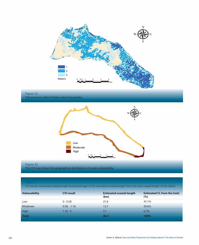
Estimates using SLR of 1 m, reveal that ~13% of the total island will be under present-day mean sea level (Table 2; Figure 10 and 11). Most of the island’s coastlines will be affected with huge eastern parts of the island submerging below the mean sea level. This was to be expected given the geomorphology of the island. The wetlands cover most of the eastern part of the island. It can also be seen that the northern coasts of the island will be affected more than the southern. This is chiefly due to the depositions of the Shat-Al-Arab region north the island. The second scenario result shows that around 46% of the total island area may disappear underwater if sea-level rises for 2 metres (Table 2; Figure 10 and 11). Naturally, even more of the island coasts will be subject by the SLR. Most of the eastern part

of the island will end up below mean sea level. In addition to the eastern region being flooded, we can see that the western part and the northern coasts will be affected strongly. The third scenario result shows that around 69% of the total island area may disappear if the sea-level rises for 3 metres. Nevertheless, two slightly elevated areas will remain above the mean sea level: (i) the first is in the middle of the island, while (ii) the second is at the south-western area of the island- close to the destroyed urban region. All of the island’s coasts will be affected strongly in this scenario, and the island will likely separate into two smaller islands (Table 2; Figure 10 and 11) The CVI results reveal that the eastern coast part will be the most subjected areas of the Island. On the other hand, the southern coast will be moderately hit by the SLR, while the northern and western coasts show the lowest vulnerability to the SLR (Figure 20, Table 3).

Scenario Peer Metres Losses Area / Km2 Percentage

Current Situation Sea level 0 46.34 100%

First Scenario 1 metre 6.14 40.2 86.75%

Second Scenario 2 metres 21.25 25.09 54.14%

Third Scenario 3 metres 31.91 14.43 31.14%

Figure 10.Areas of Failaka Island that will be lower than mean sea level in case of realization of three different SLR scenarios (1, 2 and 3 metres).


Table 3.CVI results, estimated coastal length and percentage of the estimated coastal length from the total coastal length of the island.

Figure 11.SLR scenarios reflect Failaka island topography.

Figure 12.The CVI map shows the geographical distribution of coasts vulnerability.

Vulnerability CVI result Estimated coastal length (km)

Estimated CL from the total (%)

Low 0 - 0.58 21.8 47.1%

Moderate 0.58 – 1.16 13.7 29.6%

High 1.16 - 3 3.1 6.7%

Total - 46.3 100%


4. DISCUSSION

The study results reveal the vulnerability of Failaka island to the SLR. The CVI analysis shows that the island's east coast and in general, the entire eastern part of the island, are most sensitive regarding the SLR. This is an expected result as it reflects geomorphology of the eastern part of the island. These results give us the initial idea of the island’s future. Thus, they are important for the Kuwaiti government which plans to start developing and inhabiting the island. Despite the fact that the accuracy of the model used in this study appears to be high, more accurate data, such as LIDAR data is still needed for precise locations based further estimates. The SLR projection for the 21st century, vary widely, but all of without doubt of point to the fact that sea level is rising significantly, and will certainly continue to rise by the end of 21st century. One of the three scenarios analysed may be realised by the end of this century (like the 1st one). Any plans for the development of the island should take this consideration into account, since its long-term effects could cause many financial losses, or could require the adoption of engineering solutions related to coastal zone management, which are very expensive. Therefore, SLR should be considered in future planning.

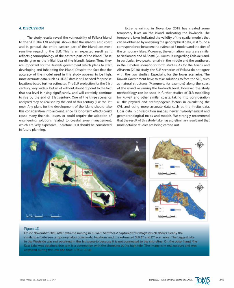
Extreme raining in November 2018 has created some temporary lakes on the island, indicating the lowlands. The temporary lakes indicated the validity of the spatial models that can be obtained by analysing the geographical data, as it found a correspondence between the estimated 3 models and the sites of the temporary lakes. Moreover, the estimation results are similar to Neelamani and Al-Shatti (2014) results regarding Failaka Island. In particular, two peaks remain in the middle and the southwest in the 3 meters scenario for both studies. As for the Alsahli and AlHasem (2016) study, the SLR scenarios of Failaka do not agree with the two studies. Especially, for the lower scenarios. The Kuwait Government have to take solutions to face the SLR, such as natural structures (Mangrove, for example) along the coast of the island or raising the lowlands level. However, the study methodology can be used in further studies of SLR modelling for Kuwait and other similar coasts, taking into consideration all the physical and anthropogenic factors in calculating the CVI, and using more accurate data such as the in-situ data, Lidar data, high-resolution images, newer hydrodynamical and geomorphological maps and models. We strongly recommend that the result of this study taken as a preliminary result and that more detailed studies are being carried out.

Figure 13.On 27 November 2018 after extreme raining in Kuwait, Sentinel-2 captured this image which shows clearly the similarities between temporary lakes (low lands) locations and the estimated SLR 1st and 2nd scenarios. The biggest lake in the Westside was not obtained in the 1st scenario because it is not connected to the shoreline. On the other hand, the East Lake was obtained due to it is a connection with the shoreline in the high tide. The image is in real colours and was captured during the low tide time (USGS, 2018).


5. CONCLUSION

Results of analysis of the three SLR scenarios indicate that ~13% of the total island area may find itself below the mean sea level for the SLR of 1 m. Most of the island’s coastal area will be affected. The eastern part of the island is the most vulnerable in regards to this scenario. For the SLR of 2 m ~46% of the total island area may disappear underwater. In addition to the eastern part, the western side will be affected noticeably too. Moreover, most of the island area will be end up underwater for the SLR of 3 m (around 69%). The CVI results reveal that the eastern part will be the most subjected areas of the Island. Studies show that the mean sea level will likely rise between 0.16 to 0.63m by 2050, and between 0.2 to 2.5 m by 2100.

ACKNOWLEDGEMENTS

The author would like to thank the ESRI, USGS, Google Earth, and the writers and institutions whose papers, websites and books were used in this study.

REFERENCES

Al-Jeneid, S. et al., 2007. Vulnerability assessment and adaptation to the impacts of sea level rise on the Kingdom of Bahrain. Mitigation and Adaptation Strategies for Global Change, 13(1), pp.87–104. Available at: http://dx.doi.org/10.1007/s11027-007-9083-8.

Al-Mutari, F., 2017. Detecting Shoreline Change of the State of Kuwait Using spatial data integration approach. Kuwait University.

Al-Sarawi, M.A. et al., 1996. Coastal Management of Failaka Island, Kuwait. Journal of Environmental Management, 47(4), pp.299–310. Available at: http://dx.doi.org/10.1006/jema.1996.0055.

Albanai, J. A., 2017. The Four Spheres “An Introduction To Physical Geography And Geosystem (2nd ed.). DAR KALEMAAT.

Aleem, K., & Aina, Y., 2013. The Use of SRTM in Assessing the Vulnerability to Predicted Sea Level Rise in Yanbu Industrial City, Saudi Arabia, (May 2013), pp. 6–10.

D’Alimonte, D. & Zibordi, G., 2003. Phytoplankton determination in an optically complex coastal region using a multilayer perceptron neural network. IEEE Transactions on Geoscience and Remote Sensing, 41(12), pp.2861–2868. Available at: http://dx.doi.org/10.1109/tgrs.2003.817682.

Alothman, A.O. et al., 2014. Sea level rise in the north-western part of the Arabian Gulf. Journal of Geodynamics, 81, pp.105–110. Available at: http://dx.doi.org/10.1016/j.jog.2014.09.002.

Alsahli, M.M.M. & AlHasem, A.M., 2016. Vulnerability of Kuwait coast to sea level rise. Geografisk Tidsskrift-Danish Journal of Geography, 116(1), pp.56–70. Available at: http://dx.doi.org/10.1080/00167223.2015.1121403.

ArcGIS Online, 2018. Basemap. Available at: http://arcgis.com.

Becker, M. et al., 2009. Impact of a shift in mean on the sea level rise: Application to the tide gauges in the Southern Netherlands. Continental Shelf Research, 29(4), pp.741–749. Available at: http://dx.doi.org/10.1016/j.csr.2008.12.005.

Intergovernmental Panel on Climate Change ed., Sea Level Change. Climate Change 2013 - The Physical Science Basis, pp.1137–1216. Available at: http://dx.doi.org/10.1017/cbo9781107415324.026.

Church, J.A. & White, N.J., 2006. A 20th century acceleration in global sea-level rise. Geophysical Research Letters, 33(1), p.n/a–n/a. Available at: http://dx.doi.org/10.1029/2005gl024826.

Church, J.A. & White, N.J., 2011. Sea-Level Rise from the Late 19th to the Early 21st Century. Surveys in Geophysics, 32(4-5), pp.585–602. Available at: http://dx.doi.org/10.1007/s10712-011-9119-1.

Cooper, H.M. et al., 2013. Sea-level rise vulnerability mapping for adaptation decisions using LiDAR DEMs. Progress in Physical Geography: Earth and Environment, 37(6), pp.745–766. Available at: http://dx.doi.org/10.1177/0309133313496835.

El-Baz, F., & Al-Sarawi, M., 2000. Atlas of State of Kuwait From Satellite Images (1st ed.). Kuwait Foundation for the Advancement of Sciences (KFAS).

El-Enin, H. A., 1989. Arabian Gulf - His bibliographic development, fluctuated sea level during the Pleistocene era. Kuwait Geographical Society, 125.

Elkhrachy, I., 2018. Vertical accuracy assessment for SRTM and ASTER Digital Elevation Models: A case study of Najran city, Saudi Arabia. Ain Shams Engineering Journal, 9(4), pp.1807–1817. Available at: http://dx.doi.org/10.1016/j.asej.2017.01.007.

Elrawy, M., 2015. Geomorphologic and Environmental Determinants for the Growth and Natural Vegetation in Kuwait. Kuwait Geographical Society, 427.

Englander, J., 2015. High Tide On Main Street (3rd ed.). Science Bookshelf.

Falour, G., Fayad, A. & Mhawej, M., 2013. GIS-Based Approach to the Assessment of Coastal Vulnerability to Sea Level Rise : Case Study on the Eastern Mediterranean. Journal of Surveying and Mapping Engineering, 1(1), pp. 41–48.

Ford, M., 2013. Shoreline changes interpreted from multi-temporal aerial photographs and high resolution satellite images: Wotje Atoll, Marshall Islands. Remote Sensing of Environment, 135, pp.130–140. Available at: http://dx.doi.org/10.1016/j.rse.2013.03.027.

Google Earth., 2018. Digital Globe Data.

Gornitz, V. M., Daniels, R. C., & White, T. W., (1994). The Development of a Coastal Risk Assessment Database: Vulnerability to Sea-Level Rise in the U.S Southern. Journal of Coastal Research, pp. 327–338.

Kumar, M., 2015. Remote sensing and GIS based sea level rise inundation assessment of Bhitarkanika forest and adjacent eco-fragile area, Odisha, 5(4), pp.674–686.

Malik, A. & Abdalla, R., 2016. Geospatial modeling of the impact of sea level rise on coastal communities: application of Richmond, British Columbia, Canada. Modeling Earth Systems and Environment, 2(3). Available at: http://dx.doi.org/10.1007/s40808-016-0199-2.

McFeeters, S., 2013. Using the Normalized Difference Water Index (NDWI) within a Geographic Information System to Detect Swimming Pools for Mosquito Abatement: A Practical Approach. Remote Sensing, 5(7), pp.3544–3561. Available at: http://dx.doi.org/10.3390/rs5073544.

McGranahan, G., Balk, D. & Anderson, B., 2007. The rising tide: assessing the risks of climate change and human settlements in low elevation coastal zones. Environment and Urbanization, 19(1), pp.17–37. Available at: http://dx.doi.org/10.1177/0956247807076960.

Meyer, B.K. et al., 2015. Shoreline dynamics and environmental change under the modern marine transgression: St. Catherines Island, Georgia, USA. Environmental


Earth Sciences, 75(1). Available at: http://dx.doi.org/10.1007/s12665-015-4780-1.

Moore, R., 2019. IPCC Report: Sea Level Rise is a Present and Future Danger. Available at: https://www.nrdc.org/experts/rob-moore/new-ipcc-report-sea-level-rise-challenges-are-growing, accessed on: 5 October 5, 2020.

Neelamani, S., & Al-Shatti, F., 2014. The expected sea-level rise scenarios and its impacts on the Kuwaiti coast and estuarine wetlands. International Journal of Ecology & Development, 29, pp. 33–43.

New Kuwait, 2018. Development Plan. Available at: http://www.newkuwait.gov.kw/, accessd on: 20 July, 2018.

Nicholls, R. & Mimura, N., 1998. Regional issues raised by sea-level rise and their policy implications. Climate Research, 11, pp.5–18. Available at: http://dx.doi.org/10.3354/cr011005.

Palmer, B. J. et al., 2011. Preliminary coastal vulnerability assessment for KwaZulu-Natal, South Africa. Journal of Coastal Research, 64, pp. 1390–1395.

Rahmstorf, S., 2010. A new view on sea level rise. Nature Climate Change, 1(1004), pp.44–45. Available at: http://dx.doi.org/10.1038/climate.2010.29.

Reyes, S.R.C. & Blanco, A.C., 2012. Assessment of Coastal Vulnerability to Sea Level Rise of Bolinao, Pangasinan Using Remote Sensing and Geographic Information System ISPRS - International Archives of the Photogrammetry, Remote Sensing and Spatial Information Sciences, XXXIX-B6, pp.167–172. Available at: http://dx.doi.org/10.5194/isprsarchives-xxxix-b6-167-2012.

Rokni, K. et al., 2014. Water Feature Extraction and Change Detection Using Multitemporal Landsat Imagery. Remote Sensing, 6(5), pp.4173–4189. Available at: http://dx.doi.org/10.3390/rs6054173.

Ryu, J. H., Won, J. S., & Min, K. D., 2002. Waterline extraction from Landsat TM data in a tidal flatA case study in Gomso Bay, Korea. Remote Sensing of Environment, 83(3), pp.442–456. Available at: http://dx.doi.org/10.1016/s0034-4257(02)00059-7.

Shaw, J. et al., 1998. Sensitivity of the coasts of Canada to sea-level rise. Available at: http://dx.doi.org/10.4095/210075.

Stevenson, J. C., Kearney, M. S., & Koch, E. W., 2002. Impacts of Sea Level Rise on Tidal Wetlands and Shallow Water Habitats: A Case Study from Chesapeake Bay. American Fisheries Society Symposium, 32, pp.23–36.

Sweet, W. V. et al., 2018. Global and Regional Sea Level Rise Scenarios.

Titus, J.G., 1990. Greenhouse effect, sea level rise and land use. Land Use Policy, 7(2), pp.138–153. Available at: http://dx.doi.org/10.1016/0264-8377(90)90005-j.

United Nations, 2017. Factsheet: People and Oceans. The Ocean Conference. New York. Available at: https://www.un.org/sustainabledevelopment/wp-content/uploads/2017/05/Ocean-fact-sheet-package.pdf.

USGS, 2018. Earth explorer. Available at: https://earthexplorer.usgs.gov, accessed on: 27 February 2018.

Sea Level Rise Projections for Failaka Island in The State ...

Documents

Transcript of Sea Level Rise Projections for Failaka Island in The State ...