SDP Memo 038: Pipeline Working Sets and Communication

SDP Memo 038:Pipeline Working Setsand Communication

Document Number . . . . . . . . . . . . . . . . . . . . . . . . . . . . . . . . . . . . . . . . . . . . . . . . . . . . . . . . . SDP Memo 038Document Type . . . . . . . . . . . . . . . . . . . . . . . . . . . . . . . . . . . . . . . . . . . . . . . . . . . . . . . . . . . . . . . . . . . . . MEMORevision . . . . . . . . . . . . . . . . . . . . . . . . . . . . . . . . . . . . . . . . . . . . . . . . . . . . . . . . . . . . . . . . . . . . . . . . . . . . . . . . . . 2Author . . . . . . . . . . . . . . . . . . . . . . . . . . . . . . . . . . . . . . . . . . . . . . . . . . . . . . . . . . . . . . . . . . . . . Peter WortmannRelease Date . . . . . . . . . . . . . . . . . . . . . . . . . . . . . . . . . . . . . . . . . . . . . . . . . . . . . . . . . . . . . . . . . . . 2017-12-14Document Classification . . . . . . . . . . . . . . . . . . . . . . . . . . . . . . . . . . . . . . . . . . . . . . . . . . . . . . . .UnrestrictedStatus . . . . . . . . . . . . . . . . . . . . . . . . . . . . . . . . . . . . . . . . . . . . . . . . . . . . . . . . . . . . . . . . . . . . . . . . . . . . . . . . . Draft

Lead Author Designation Affiliation

Peter Wortmann Research Associate University of Cambridge

Signature & Date:

Revision Date of issue Prepared by Comments

1 2017-12-01 Peter Wortmann Initial publication

2 2017-12-14 Peter Wortmann Revised calibration after discussion withStefano Salvini and Tim Cornwell

SDP Memo Disclaimer

The SDP memos are designed to allow the quick recording of investigations and research doneby members of the SDP. They are also designed to raise questions about parts of the SDPdesign or SDP process. The contents of a memo may be the opinion of the author, not thewhole of the SDP.

Table of Contents

1 Introduction 31.1 Motivation . . . . . . . . . . . . . . . . . . . . . . . . . . . . . . . . . . . . . . . 31.2 Assumptions . . . . . . . . . . . . . . . . . . . . . . . . . . . . . . . . . . . . . 4

2 Visibilities 52.1 Visibility Rates . . . . . . . . . . . . . . . . . . . . . . . . . . . . . . . . . . . . 52.2 Time to Work . . . . . . . . . . . . . . . . . . . . . . . . . . . . . . . . . . . . . 62.3 Streaming . . . . . . . . . . . . . . . . . . . . . . . . . . . . . . . . . . . . . . . 62.4 Stream Processing . . . . . . . . . . . . . . . . . . . . . . . . . . . . . . . . . . 7

3 Continuum Imaging 83.1 Sub-Band Split . . . . . . . . . . . . . . . . . . . . . . . . . . . . . . . . . . . . 83.2 Cost of Distribution . . . . . . . . . . . . . . . . . . . . . . . . . . . . . . . . . . 93.3 Distribution Options . . . . . . . . . . . . . . . . . . . . . . . . . . . . . . . . . 93.4 Facetting Working Set . . . . . . . . . . . . . . . . . . . . . . . . . . . . . . . . 113.5 Parallelism . . . . . . . . . . . . . . . . . . . . . . . . . . . . . . . . . . . . . . 113.6 Distributing Further . . . . . . . . . . . . . . . . . . . . . . . . . . . . . . . . . . 123.7 Communication . . . . . . . . . . . . . . . . . . . . . . . . . . . . . . . . . . . . 123.8 Streaming Order . . . . . . . . . . . . . . . . . . . . . . . . . . . . . . . . . . . 143.9 Implementation Sketch . . . . . . . . . . . . . . . . . . . . . . . . . . . . . . . . 16

4 Calibration 164.1 Challenges . . . . . . . . . . . . . . . . . . . . . . . . . . . . . . . . . . . . . . 164.2 Implementation Options . . . . . . . . . . . . . . . . . . . . . . . . . . . . . . . 174.3 Streaming Calibration . . . . . . . . . . . . . . . . . . . . . . . . . . . . . . . . 17

4.3.1 Alongside Imaging . . . . . . . . . . . . . . . . . . . . . . . . . . . . . . 174.3.2 Pre-Processing . . . . . . . . . . . . . . . . . . . . . . . . . . . . . . . . 18

4.4 Global Calibration . . . . . . . . . . . . . . . . . . . . . . . . . . . . . . . . . . 194.5 Calibration Data . . . . . . . . . . . . . . . . . . . . . . . . . . . . . . . . . . . 194.6 Aggregation . . . . . . . . . . . . . . . . . . . . . . . . . . . . . . . . . . . . . . 214.7 Communication . . . . . . . . . . . . . . . . . . . . . . . . . . . . . . . . . . . . 224.8 Distribution . . . . . . . . . . . . . . . . . . . . . . . . . . . . . . . . . . . . . . 23

Document no.: SDP Memo 038Revision: 2Release date: 2017-12-14

UnrestrictedAuthor: Peter Wortmann

of 30

5 Spectral Pipelines 235.1 Working Set . . . . . . . . . . . . . . . . . . . . . . . . . . . . . . . . . . . . . . 235.2 Communication . . . . . . . . . . . . . . . . . . . . . . . . . . . . . . . . . . . . 245.3 Data Products . . . . . . . . . . . . . . . . . . . . . . . . . . . . . . . . . . . . 25

6 Conclusion 256.1 Data Flow . . . . . . . . . . . . . . . . . . . . . . . . . . . . . . . . . . . . . . . 266.2 Summary . . . . . . . . . . . . . . . . . . . . . . . . . . . . . . . . . . . . . . . 27

References 27

List of Symbols 27

List of Figures 29

List of Tables 29

1 Introduction

The pipelines of the SKA SDP are clearly very data intensive: Even for a large cluster the inputrate of 0.4 TB/s is not trivial to absorb and process. However, the real problem emerges incombination with the nature of imaging and calibration. Serving such astronomical algorithmsinvolves extracting as much information as possible from the input data concerning certaintime slot, frequency channel, or sky directions. Unfortunately, this generally boils down toexceptionally large queries into the already-large data sets. In fact, imaging is the worst casehere, as basically every single input visibility contains a certain amount of information aboutany given sky direction.

This means that we have to be extremely careful with how exactly we move the data throughthe system. Algorithms that appear trivial on paper can easily turn out to be basically impossibleto implement because of the data reorganisation involved. Worse, effective self-calibrationpipelines involve running many different types of demanding imaging and calibration algorithmswithout much common ground in terms of access or aggregation patterns. So unless we proveotherwise, it would seem likely that we might run into subtle incompatabilities down the road.

For this memo, we will therefore focus on these data reorganisations and aggregations andattempt to show that we can move data around in a way that

• we never run out of working memory,

• we never exceed communication limits, and

• we actually finish within in the designated time.

We will see that these goals are in strong competition with each other. However, characterisingthese trade-offs exactly yields us a lot of useful restrictions on both algorithm choice as well asthe mapping to the compute hardware. By the end of this memo, we will have restricted thedesign space enough to arrive at some pretty concrete recommendations.

1.1 Motivation

As a starting point, consider that 0.4 TB/s of input visibility data adds up to about 1.4 PB of dataper hour. So if we assume to have roughly 1400 compute nodes available, this means that even



of 30

holding just this short observation in memory would require around 1 TB of working memory.And it gets worse: For calibration and deconvolution we would need to predict model visibilitiesto compare with the measurement data, which might multiply the amount of visibility data upquite a bit further. And this is even before we starting considering images and calibration data.

So unless we get strategic with how we handle data, this could easily multiply up the workingto multiple TB worth of data, with no obvious upper bound in sight. This actually seems to be avery real trend with current telescopes: The processing model of the SKA precursor MeerKATplaces key functions on four nodes with RAM in the Terabyte scale. Similar things seem to behappening for the Askap precursor as well.

For the Science Data Processor this is clearly a problem, as we need to do this on a muchlarger scale. Even for 2022 hardware Graser (2016) does not budget for more than 500 GB ofmemory per node. The ability to run SDP pipelines on this sort of hardware is clearly not goingto happen by accident, we need guarantees.

1.2 Assumptions

Before we start with the main body of the memo, let us get a few assumptions out of theway. The numbers for this analysis are based chiefly on parametric model (Bolton et al., 2016)predictions for data sizes and compute complexity.

We especially adopt the parametric model nomenclature of grouping pipelines producingimages as “imaging pipelines”, even if they consist of prediction as well as invert steps. Thisis convenient as predict and invert is mostly symmetric if we consider FFT-based methods tobe required – which we should at the targeted scale of the SKA. In the following, when wetalk about imaging we are therefore referring to the FFT predict/invert pair with all supportinginfrastructure such as reprojections, facet splits, phase rotation, gridding and degridding.

However, we make a number of assumptions on top of the parametric model:

• We assume that for continuum imaging we use three Taylor terms, so Ntt = 3. After talkingwith several astronomers, this seems to be a more realistic choice than the original valueof Ntt = 5, see for example discussion in Nikolic et al. (2016). We will see that this numberscales basically everything, so we have to choose it carefully.

• Normally the parametric model implicitly allows a pipeline to run for as long as the lengthof the observation, reflecting a “steady state” model of operation. However, in realitywe will want to run more than just a single pipeline on the observation data, thereforewe introduce a top-level factor Qspeed that scales the time we have to finish processingrelative to the length of the observation.

• We will fix the snapshot length at tsnap = 600s. Background is that we expect to behandling w-terms using a mixture of w-stacking as used by Offringa et al. (2014) andw-snapshots (Cornwell et al., 2012). This should make it much easier to choose snapshotsize for architectural reasons, and a value around ten minutes seems to work well.

Furthermore, throughout this memo we will only consider the Mid1 band for the SKA1 Midtelescope. This is because all Mid bands generally behave very similarly for the purpose of theSDP, with the Mid1 band the narrow cost leader. See Table 4 at the end of the document for fullnumbers.



of 30

“Danger Zone”

Predict Buffer

Model Vis Measured Vis

Solve Image

Solutions

Residual

Clean

Components

Lessdata

intensive

Figure 1: Continuum Pipeline Major Loop Structure

2 Visibilities

Sadly, the working set size we alluded to in subsection 1.1 is not a fantasy: As Figure 1 shows,a major loop iteration is a linear data reduction process with a very “top-heavy” structure. Thereare no natural synchronisation points that would suggest that we are “done” with a given typeof data entirely. So a naıve execution of the pipeline might use too much of the availableparallelism (a well-known effect in programs with a data flow representation, see Culler andArvind, 1988), and therefore stay in the dangerous zone for too long.

Note that in Figure 1 we have drawn this zone to end mostly with visibilities. The reasoningis that both images and calibration solutions are less problematic, as they can be aggregatedrather aggressively. We will explore that in detail in section 3 and section 4 respectively. Animportant exception here is extreme spectral pipelines (like DPrepC), for which we cannotaggregate images as much. We will have a closer look at that case in section 5.

2.1 Visibility Rates

So let us return to the visibility working set argument from the Motivation section. What areour tolerances here exactly? We know that we will have to loop over all data at minimumNmajor times for the major loop, and we will likely have to do it faster than we received the dataoriginally. So we know that in Figure 1 the measured visibility data will be read from the bufferat the following rate per node:

Rvis/node =RvisQspeedNmajor

Nnode≈ 4.414GB/s for SKA1 Low

≈ 4.805GB/s for SKA1 Mid1



of 30

If we assume that we need to produce Npredict separate model visibilities at the same time –such as for major loop subtraction or calibration – model visibilities will contribute an even moresignificant influx of data. The amount of prediction needed clearly depends on the experiment,but even with just Npredict = 4 this would add up to:

Rpredict/node = NpredictRvis/node ≈ 17.65GB/s for SKA1 Low≈ 19.22GB/s for SKA1 Mid1

2.2 Time to Work

From this we can now easily calculate how much memory we need to be able to “work” on agiven piece of data for a certain time:

Mvis/node = twork(Rpredict/node +Rvis/node)

twork =Nnode

Rpredict/node +Rvis/node

Let us assume that we can allocate 64 GB of node memory for storing visibilities, this yields us2.83 s (Low) or 2.92 s (Mid1) respectively for leaving the “danger zone” before memory runsout. This is a very small amount of time, given that:

• This must include time needed for either generating the data, or loading it from eitherstorage or over network

• There must be some slack due to imperfect scheduling or congestion

• All computation on that data must be finished before the time runs out

We can extend this time window by increasing node memory. We can actually easily calculatethe cost of that: At a price of memory of 0.5 e/GB extending this time window by a secondwould add roughly 15000 e/s to the budget (and 4.5 kW assuming 0.3 W/GB) (Graser, 2016).

2.3 Streaming

This heavily suggests a “streaming” kind of processing model for visibilities: Explicitly work in asequential fashion, aligned with the order that data gets loaded into memory. So ideally, wewould:

1. Stream visibilities in from the buffer

2. Predict alongside, synchronised using e.g. back-pressure (see subsection 3.9)

3. Do low-latency local processing

4. Output “processed” visibility data into a number of output buffers

5. Discard raw visibilities

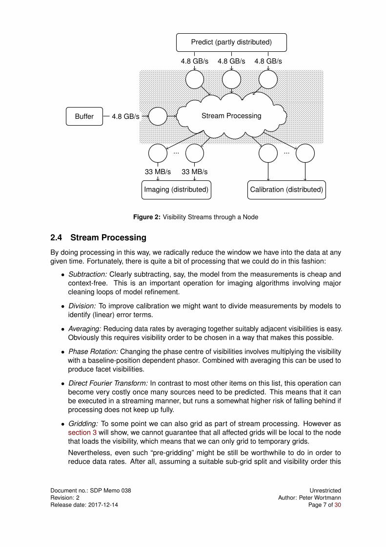
Keeping these processes in alignment will require some careful intermediate caching as shownin Figure 2. This is especially important because as we will see, prediction, imaging andcalibration can not be distributed in a way that aligns with visibility streaming.



of 30

Buffer

Predict (partly distributed)

Stream Processing

... ...

Imaging (distributed) Calibration (distributed)

4.8 GB/s

4.8 GB/s 4.8 GB/s 4.8 GB/s

33 MB/s 33 MB/s

Figure 2: Visibility Streams through a Node

2.4 Stream Processing

By doing processing in this way, we radically reduce the window we have into the data at anygiven time. Fortunately, there is quite a bit of processing that we could do in this fashion:

• Subtraction: Clearly subtracting, say, the model from the measurements is cheap andcontext-free. This is an important operation for imaging algorithms involving majorcleaning loops of model refinement.

• Division: To improve calibration we might want to divide measurements by models toidentify (linear) error terms.

• Averaging: Reducing data rates by averaging together suitably adjacent visibilities is easy.Obviously this requires visibility order to be chosen in a way that makes this possible.

• Phase Rotation: Changing the phase centre of visibilities involves multiplying the visibilitywith a baseline-position dependent phasor. Combined with averaging this can be used toproduce facet visibilities.

• Direct Fourier Transform: In contrast to most other items on this list, this operation canbecome very costly once many sources need to be predicted. This means that it canbe executed in a streaming manner, but runs a somewhat higher risk of falling behind ifprocessing does not keep up fully.

• Gridding: To some point we can also grid as part of stream processing. However assection 3 will show, we cannot guarantee that all affected grids will be local to the nodethat loads the visibility, which means that we can only grid to temporary grids.

Nevertheless, even such “pre-gridding” might be still be worthwhile to do in order toreduce data rates. After all, assuming a suitable sub-grid split and visibility order this



of 30

allows us to reduce data density to one “visibility” per grid cell, and allows us to possiblyaggregate grid data from baselines that are close in uv-space1. We will touch on thisagain in subsection 3.8.

• Degridding: Dual to gridding, if a grid is available we can degrid predicted visibilities fromit. This is the cheaper and less accurate alternative to direct Fourier transforms, but justas with gridding requires appropriate grid data to be made available.

• Calibration: Up to a certain point we can solve for calibration on streaming visibilities.Because of the limited window this will have to be very limited in scope, and it seemslikely that we would only be able to calibrate out very clear signals this way. We will lookmore closely into this idea in subsection 4.3.

So in fact, quite a few of the important operations of radio astronomical pipelines work wellwith small data windows. The two main exceptions we had to make were de/gridding andcalibration. The underlying reason is of course that by design grids, images and calibrationproblems correspond to large windows of visibility data. Therefore we need scatter and gatheroperations around the sketched stream processing. This leads to new working set problems,which we will investigate in the next sections.

3 Continuum Imaging

Processing as discussed so far is so “embarrassingly” parallel that it puts basically no restric-tions on the order we process visibilities. This is in stark contrast to imaging pipelines, whichimpose strong locality requirements on loading and producing data. This means that we needto have a serious look into how we can distribute this processing under the assumptions derivedso far. The hardest case here is the self-calibration pipeline ICAL, as in contrast to spectralpipelines it is meant to identify components and solve calibrations in relatively coarse frequencywindows. This makes it a hard pipeline to distribute effectively. Furthermore, the requirementto image to the third null of the beam yields large images, which blows up the working set sizesignificantly.

So clearly we need to consider imaging locality at least a secondary goal here. To beconcrete, we need to check that the data distribution assumptions we just made about visibilitieswill not make it impossible to deal with the second most data-intensive data object in our pipeline:Raw images and and their underlying grids.

3.1 Sub-Band Split

Despite it being a relatively coarse split compared with spectral pipelines, the most low-hangingfruit here is still the frequency axis. After all, this is where visibility and image locality align:Simply by “pinning” workers to a band we reduce the amount of image information any singlenode has to care about. If visibility data is distributed accordingly, this is basically free2.

1Thanks to Bram Veenboer for noting this!2In fact, if we worked on sub-bands sequentially, we could even spill sub-band images to disk. This is actually

exactly what we are going to do for the spectral pipelines considered in section 5. Yet for continuum pipelines weare actually somewhat short on “cheap” parallelism, so we do not consider that option here.



of 30

However, this is not enough by far – even just the image for one frequency sub-band isalready very heavy. We can calculate:

NttNppMimage = NttNppMpxN2pix,total

≈ 0.278TB for Low ICAL≈ 14.23TB for Mid1 ICAL

Assuming Ntt = 3. This is clearly still too much for a node to aggregate locally. Unfortunately,in terms of the global working set this is actually already the end of the line: No matter howwe turn the problem, every visibility eventually impacts this exact amount of grid/image data.Therefore streaming visibilities requires this amount to be held in memory somewhere.

While we cannot reduce the global working set, we can still reduce the working set per nodeby distributing the load. After all, at this point our distribution degree is just Nsubbands = 7 (Low)or Nsubbands = 4 (Mid1) respectively, which is by far not enough parallelism to use a large-scalecompute facility effectively.

3.2 Cost of Distribution

So we require more distribution, both to split computational cost and to reduce the workingset. Unfortunately, no other distribution option is quite as “embarrassingly parallel” as splits bysub-band. No matter what we do, we have to incur additional cost in some form. Those costsare, in rough order of badness:

Work: In some cases the split might not simply be about selecting or weighting visibilities, butmight involve significant computational splitting/merging work. In that case we have to becareful that we do not introduce a new computational bottleneck into the pipeline.

Communication: We generally assume that visibilities will be distributed “optimally” acrossnodes before we start processing. However, for some distributions the same chunk ofvisibility data might still end up as a data dependency for different nodes. This requiresus to introduce node communication. Depending on how many nodes take part in thedistribution, we might even be forced to exchange data between compute islands.

Note that on paper, we might consider cutting down communication cost by duplicatingvisibility data in the buffer. However, this would directly increase both hot buffer capacityand bandwidth. Furthermore, in practice this would duplicate all visibility stream process-ing discussed before (including direct Fourier transforms and phase rotation). This wouldbecome prohibitively expensive pretty much immediately.

Working Set: Finally we might fall back to having copies of the grid/image that can be updatedor predicted from independently. For the purpose of this analysis, this is going to be ourlast resort once we reach the limits of what our architecture can otherwise support.

3.3 Distribution Options

Fortunately, the Fourier transformation underlying imaging is a rather malleable method. AsTable 1 shows, we can split along quite a number of axes:

• Direction: Imaging with a different phase centres still requires covering the whole uv-gridwith visibilities, leading to an all-to-all communication pattern as shown in Figure 3.



of 30

Axis Size Extra Work Communication Working SetFrequency (subband) 4-7 none none constantPolarisation (separate) 2-4 none none constantDirection (facet) flexible phase rotation roughly constant constantPolarisation (cross) 2-4 none linear constantTaylor terms 2-5 none linear constantFrequency (rest) flexible none none linearTime (snapshot) 3-36 none none linearBaseline flexible imbalances? none linear?

Table 1: Continuum Imaging Distribution Options

Stream

Buf

Grid/FFT

Stream

Buf

Grid/FFT

Stream

Buf

Grid/FFT

Stream

Buf

Grid/FFT

Figure 3: All-to-all Distribution Pattern of Facets, Polarisations and Taylor Terms

This might seem highly undesirable, but fortunately the reduced field of view per facetreduces sampling requirements in the uv-grid, which means that we can average visibilitiesmore aggressively. This mostly offsets the fact that we need to produce visibility sets perdirection: In Figure 3 every arrow only carries data roughly 1

16 the size of the total visibilitydata. The amount of network transfer is effectively the same as if we were re-shuffling allvisibility data between the nodes once.

However, the phase rotation and averaging operations required for producing visibilitiesfor a facet field of view are not free: The obvious implementation would scale quadraticallywith the number of facets, which can easily introduce significant costs. There might besome optimisation potential here – such as employing FFTs or a direct divide-and-conquerapproach – but there is always going to be cost.

• Polarisation: Without cross-polarisation terms, this would actually be another “embarrass-ingly” parallel distribution axis just like sub-bands. However, the assumption is that weneed to account for those terms, which means that the image for any given polarisationwould require the visibility data for all input polarisations.

This introduces the same communication patterns as illustrated in Figure 3, yet in contrastto facets we have no easy in-built mechanism for data reduction. Therefore distributing inpolarisation scales up the amount of network transfer in a linear fashion.



of 30

• Taylor Terms: Based on weighted visibilities, therefore needs all visibilities when dis-tributed. This leads to the same kind of communication as distribution in polarisation.

• Time: Outside of fast imaging (which we do not consider here), no pipeline producesimages split by time, so any distribution would increase working set size by preventingaggregation.

We might still want to distribute along this axis simply because it naturally aligns with howvisibilities are measured and snapshot imaging operates. While this will increase workingset size, it provides a flexible way to scale node load without a lot of communication.

• Baseline: Dual to faceting – accumulate portions of the uv-grid. While this is a verynatural choice for optimising visibility data locality, this makes balancing work harder, asvisibility density varies a lot over the uv plane. Furthermore, in contrast to images uv-gridscan not trivially be accumulated across projection changes (as with w-snapshots).

Therefore this basically requires a full time split (or a second-stage re-distribution), whichwould seem to eliminate the benefit. We will however consider this topic again whenconsidering sequential computation order in subsection 3.8.

3.4 Facetting Working Set

Clearly direction (faceting) is the most promising distribution axis here. If we follow parametricmodel (Bolton et al., 2016) recommendations for sizing, for Mid1 we can cover the field of viewto the third null of Mid1 with 7×7 facets without having too pay too much for phase rotation.This also fits fairly well into the island size of Nisland = 56 (Graser, 2016).

This would reduce the amount of image data every node has to hold to:

Mimage/node,max =MimageNppNtt

N2facet

≈ 8.17GB [Low ICAL]≈ 290.5GB [Mid1 ICAL]

Which is not enough for SKA1 Mid, so we have to look further.At this point we might be tempted to use local storage to off-load some of this working set.

If we assume that we need to write a whole image out after every snapshot (for tsnap = 600s),this would result in the following write rates:

Rimage =NmajorQspeedMimage/node,max

tsnap

≈ 0.204GB/s [Low ICAL]≈ 7.263GB/s [Mid1 ICAL]

Unfortunately, the point where the working set becomes problematic coincides with the pointwhere we go past the hot buffer read rate. As a high write rate is somewhat harder to achievecompared with a high read rate, we must take this seriously – spilling does not help us here.

3.5 Parallelism

If we assume that the cluster will have Nnode ≈ 1500 nodes with Nsubbands = 7 (Low) andNsubbands = 4 (Mid1) this means we would want to aim for Nnode ≈ 218 (Low) or Nnode ≈ 334



of 30

(Mid1) respectively in order to have enough parallelism. This means that assuming a simple7× 7 facet split as recommended by the parametric model provides around 4-7 times lessparallelism than we require.

Note that an alternative strategy here might be to reduce Nnode by splitting compute re-sources between processing blocks (Nikolic and Bolton, 2016). This would require increasinghot buffer capacity, but not hot buffer bandwidth, as computation could take a longer timeto finish. However, while this might introduce enough parallelism from the top level, it wouldnot help with the working set problem: Every node would still have to hold all polarisationsand Taylor terms for a facet. So this does not work well for pipelines involving high-resolutionimages such as SKA1 Mid.

3.6 Distributing Further

At this point, we have run out of “easy” choices. We might simply choose to use more facets,yet 14×14 or 19×19 facets would add significant phase rotation costs (roughly 1-2 Petaflopsper second). So alternatively let us try splitting by another distribution axis mentioned in Table 1.There are only two classes of options left:

• Reduce working set per node at the expense of communication by increasing distributionin Taylor terms or polarisation.

• Keep communication constant at the expense of global working set size by distributing intime or frequency.

As two of the distribution axes each are the same for our purposes, let us say that we have acombined distribution degree of Ndist,pp,tt in either polarisation and Taylor terms (or both), and acombined distribution degree of Ndist,f,t in either time or frequency (or, again, both). If we wantexactly enough parallelism to keep Nnode nodes busy, we can calculate them from each other:

Ndist,f,t = max

{1,

Nnode

NsubbandsN2facetNdist,pp,tt

}This allows us to scale the working set size per node quite a bit, potentially until the point whereevery node only has one facet worth of image data to keep track of for every node:

Mimage/node = max{

Ndist,f,tNsubbandsNppNttMimage

Nnode,Mfacet

}See the solid lines in Figure 4 for values depending on the value of Ndist,pp,tt (and thereforeNdist,f,t). It is clear that we can reduce the working set per node significantly by distributing inpolarisation and Taylor terms. Note that because of the different number of subbands we runinto the lower working set limit at different points for Low and Mid1.

3.7 Communication

Reducing the working set like this is clearly very desirable. However, as noted before we willneed more communication to make it happen. After all, now we need to copy the facet visibilitiesbetween nodes a few times. In fact, we can easily see that this requires communication with allnodes except those working on a different block in time and frequency, which means it worksout as:

Ncopy =Nnode

Ndist,f,tNsubbands= min

{Nnode

Nsubbands,N2

facetNdist,pp,tt

}



of 30

1 2 3 4 5 6 7 80

50

100

150

200

250

300

0

2

4

6

8

10

12

Ndist,pp,tt

Mim

age/

node

[GB

]

Rim

agin

g/no

de[G

B/s

]

LowMid1

Figure 4: Imaging Working Set and Communication per Node (for 7×7 facets)

This means that if we have Rvis,facet as the total averaged visibility rate for a facet, we cancalculate the communication of every node as:

Rimaging/node = (Ncopy−1)QspeedRvis,facet

Nnode

Results depending on the value of Ndist,pp,tt are shown in Figure 4 as dashed lines. As shouldbe expected, every increase of Ndist,pp,tt corresponds to an increase of network I/O in the sameorder of magnitude as the visibility rate.

Especially note that this communication would be between Ncopy nodes in an all-to-allfashion as illustrated back in Figure 3. This means that once the value of Ncopy passes thenumber of nodes that a compute island contains (we assume Nisland = 56) communication musthappen between compute islands.

We can calculate the rate every island would have to emit in a fashion similar to Rimaging/node:

Rimaging/island = (Ncopy−Nisland)NislandQspeedRvis,facet

Nnode

As Figure 5 shows, once Ncopy passes Nisland this adds up rather quickly. This is traffic emittedper island, so for over 20 islands what we are seeing here is global traffic blow way past 10 TB/s.

However, note that traffic between each given pair of islands involved in the all-to-all isroughly constant independent of Ndist,pp,tt and given by:

Rimaging/island2island =N2

islandQspeedRvis,facet

Nnode

≈ 46.72GB/s for SKA1 Low≈ 94.23GB/s for SKA1 Mid1

So whether or not this is possible might depend exactly on whether we can sustain thissort of data rate between islands. It will likely take some careful hardware planning andexperimentation to figure out the most workable compromise here.



of 30

1 2 3 4 5 6 7 80

100

200

300

0

100

200

300

400

500

Ndist,pp,tt

Nco

py

Rim

agin

g/is

land

[GB

/s]

LowMid1

Figure 5: Imaging Island Communication (for 7×7 facets)

3.8 Streaming Order

We have covered how we could distribute the image data across nodes in order to minimiseworking set size and communication. However, to make streaming work as explained insubsection 2.3, we also need to show that we have a viable order in which we can processthe visibilities without the working set blowing up further. Fortunately, sequential distributionhas the significant advantage that we can aggregate in-place somewhat cheaply. We can splitvisibilities almost arbitrarily much in frequency, time and baseline without impacting our abilityto work with the resulting chunks.

The main exception is snapshots: Clearly we would want to work in a way that not toomany snapshots are worked on at the same time, as that would multiply up the amount ofimage/grid data that needs to be in memory at the same time. This means we will want to“softly” synchronise nodes collaborating on an imaging task: The grids for predict and imaginga certain snapshot should become available just as the first node requires them. Note that theoverhead due to this is going to be lower the larger snapshots are.

Furthermore as noted in subsection 3.3, we might have to be quite picky with how wechoose visibility order to optimise de/gridding. After all, w-stacking would become eithermemory inefficient or require many redundant FFTs unless we cluster visibilities that areclose in uvw space together. This would even allow us to move gridding work on the orderside of the communication, replacing phase-rotated visibilities with sub-grids.3. This is avery attractive design point: Even taking baseline-dependent visibility averaging into account,transferring gridded visibilities seems like it could decrease required communication by anorder of magnitude. As illustrated in Figure 6, this suggests a very concrete way to distributeand stream visibilities: After initial chunking to some chosen granularity in baseline, time and

3Obvious choice would be to account for anti-aliasing, A-terms and fine w-terms on the streaming side. The nodeholding the image data would take care of coarse w-terms using w-stacking. Note this also has the nice propertythat most A-patterns are only required on very few nodes.



of 30

t = 0 t = 1 t = 2 t = 3

Figure 6: Sequential Work Order across Snapshot Grids

FFT/Degrid

Stream

Buf

Grid/FFT

FFT/Degrid

Stream

Buf

Grid/FFT

FFT/Degrid

Stream

Buf

Grid/FFT

FFT/Degrid

Stream

Buf

Grid/FFT

Speed up! Slow down!Speed up! Slow down!Speed up! Slow down!Speed up! Slow down!

Skip!

Figure 7: Back-pressure Throttling of Predict

frequency4, we order visibilities first by snapshot, then by position in the uv(w)-grid. Then wewould “stripe” the visibility chunks for this order into distributed storage, so that neighbouringvisibilities will be loaded at roughly the same time.

Making the work order entirely deterministic makes the whole system very easy to describein terms of streams: Facet prediction processes will stream visibilities (degridded or not) tothe visibility processes in exactly the required order, and on the flip side nodes holding facetdata will receive grid contributions back in the same predictable order. This especially makes itrelatively straightforward to load-balance computation and communication. This is a criticallyimportant feature for SDP: Remember that for predict, we want to generate visibilities just asthe measured visibilities get loaded from the buffer. Clearly the cluster collectively must bepowerful enough to supply model visibilities at a higher rate than we can read visibilities fromthe buffer. Therefore there is the real risk that we might overwhelm visibility processing.

4A-kernel scopes are the obvious lower bound. Concrete granularity should depend on visibility density in uv-grid.



of 30

3.9 Implementation Sketch

The standard solution here seems to be to use back-pressure type mechanisms (Collins andCarloni, 2009) as shown in Figure 7 to throttle predict to match the buffer rate:

• Once we reach a high water mark on predicted visibilities, start throttling predict.

• When we reach a low water mark on predicted visibilities, reduce predict throttling.

Note that this balancing process would have to be “democratic”, as every predict has multipleconsumers potentially running at slightly different speeds. This means that it is impossible totruly prevent buffer over- or underflows. Fortunately though, most of the streaming visibilitydata is “non-precious”, so we can actually exhaustively deal with all possible situations:

• If predicted visibilities overflow, this means we stop accepting predicted visibilities, thenjump over buffer visibilities. This will allow the buffer and processing to catch up.

• If we actually run out of data on a buffer, the kernel will have to wait. This might causeother input buffers to overflow and skip data using the same mechanism.

This could be combined with additional load-balancing techniques, but it is likely that our dataflows are predictable enough that this would be needed only rarely. In the end, the SDP shouldlikely prioritise raw I/O at the prize of the risk of some data loss here.

4 Calibration

Outside of refining the sky model, the other primary reason for running the self-calibrationpipeline is to find improved calibration solutions. This is a very complex topic, but the generalgoal is always to calibrate out a certain bias, generally per antenna / station:

• Bandpass: Fine calibration for sensitivity in specific frequencies

• Gains: Phase errors of the visibility

• Pointing: Errors in primary beam position

• Ionosphere: Various delays due to the beam passing through the ionosphere

While there are many different types of calibration, the principle seems to stay the same: Weobtain a model for what we expect visibilities to be, which we then compare with the observedvisibilities. We then proceed to tease apart the bias from other calibration effects or – worse –the signal. This is done by strategically comparing, grouping and averaging the measured andmodel visibilities until enough proof for systematic errors is found.

4.1 Challenges

Unfortunately, the practice of calibration is somewhat at odds with the restrictions on data flowas we have explained them so far. There are two main problems here:

Firstly, there is often significant overlap between calibrations. For example, gain errorsonly differ from ionospheric errors by how and how quickly we assume them to change in time,frequency and direction. Worse, even the same types of calibrations might have non-trivialinteractions: As long as we have not obtained a precise calibration into the direction of a bright



of 30

source, the errors of that miscalculation might throw off all calibration on calibrators in thegeneral vicinity.This leads to algorithms like LOFAR’s facet calibration (Van Weeren et al., 2016),which calibrates facets entirely sequentially. This is a problem for our architecture, because asestablished in subsection 2.3 we can not actually “go back” very often – the system is sized forreading visibilities just about a few dozen times across its lifetime in offline processing.

Furthermore, for calibration to work effectively we must achieve as much signal-to-noise aswe can. This means that we want to involve as many visibilities as possible: For high-qualitybandpass calibration we would ideally want to take all visibility data that applies to a certainfrequency range into account. Unfortunately, by nature different calibrations will want to slicedata in entirely different ways: Just as bandpass calibration requires large time windows butsmall frequency windows, gain calibration would want small time windows, yet relatively largefrequency windows.

4.2 Implementation Options

Viewed in isolation there is no “right” data distribution for visibility data: Every possible choiceforces at least one calibration to perform a – possibly even global – redistribution of calibrationdata before we can solve it. This makes it hard to fit into a situation where we want to streamvisibilities through under high memory pressure like with predict and invert.

This restricts our design space to two distinct algorithmic options:

1. Adopt the order the visibilities are streamed in, and therefore accept extremely limiteddata windows dictated by memory pressure. This forces calibration into the same workingorder as either imaging or ingest, which restricts the types and quality of calibration.

2. Commit to a data reorganisation with heavy aggregation in order to not exhaust memory.This also means large delays for actually obtaining and applying solutions, as collectingall required input data might take a full major loop.

We will look at these two options in detail in the next two sections.

4.3 Streaming Calibration

Let us first consider the option of calibrating within a given visibility stream. While such acalibration might have access to some “wisdom” from visibilities earlier in the stream, previouscalibration runs or (non-guaranteed!) other calibration processes running in parallel – the onlydata window it is really guaranteed to have is what it happens to find in the streaming cache.

The good news is that such streaming calibration has unrestricted access to full-accuracyvisibility data. This especially means that it could iterate and stack calibration methods on topof each other as much as the processing budget allows. This might be the appropriate way toimplement calibration methods such as peeling (Intema et al., 2009) for sources that are brightenough to detect in any visibility snapshot of sufficient size (such as the A-team?).

A significant advantage of such sequential calibration is that we do not need to worry aboutcalibrating out effects twice: We can apply the calibration right after it was solved, and do nothave to worry about residual effects confusing other calibration solvers.

4.3.1 Alongside Imaging

Pairing streaming calibration with imaging might not look too problematic on first glance: Weexpect to have around 64 GB of data to work with, that should allow us to do something, right?However, if we take a closer look back at subsection 3.8, things become a bit more tricky.



of 30

We said that we would expect visibilities to be traversed by snapshot, then by region inuv-space. The former is good, as we would likely stream the types of calibration that arevery localised in time anyway. However the latter is very bad, as calibration typically requiresvisibilities for all baselines, which by design are very spread out over the uv grid. If we assumethat we only re-visit a certain region on the grid for every snapshot with tsnap = 600 s, this meanswe need to hold an entire snapshot worth of visibilities in working memory for:

twork,snap =tsnap

QspeedNmajor≈ 40s

which compares unfavourably with twork < 3s, the time we gave visibilities to stay memory-resident in subsection 2.2. We can easily calculate that in order to give calibration a windowlarge enough to cover a snapshot we would have to hold:

Msnap/node =QspeedNmajorNppRvistsnap

Nnode

≈ 183.60GB [SKA1 Low]≈ 175.29GB [SKA1 Mid1]

Note that in contrast to the calculation in subsection 2.2 we now assume that we do not needto hold model visibilities for this long, which is why this looks less crass. This mostly rulesout distributed predict, and therefore effectively limits us to model visibilities generated byjust-in-time direct Fourier transforms – which seems appropriate in this case.

However, this is still a very significant amount of data, especially considering that this wouldhave to be added on top of all previously mentioned visibility buffering. We might be able toimprove this number by choosing smaller snapshots, or – equivalently – make multiple passesthrough the grid (both would introduce more FFT cost). Also note that this would restrict howwe could stripe visibility data among nodes, as we need to make sure that every one has acomplete set of baseline visibilities to solve calibration for a certain slot in time and frequency.

These are quite thorny requirements – it should illustrate why calibration is such a problemfor our architecture. However, it might still be worth the price: For SKA1 Low we have relativelysmall imaging working sets, and exceptionally tough calibration problems. So setting aside200 GB of visibility re-ordering buffer per node for calibration should not be dismissed.

4.3.2 Pre-Processing

If we take a broader look of the life cycle of visibilities, during continuum imaging might well bethe worst time to try to do streaming calibration. Remember that visibilities are also naturallyingested in a streaming fashion – in an order that is much less problematic for calibrationsolving. After all, we need to be able run the real-time calibration pipeline (RCAL)!

This heavily suggests that calibrations that do not need distributed predict should be solvedbefore we even enter the self-calibration pipeline. We have a good number of options for doingthat within the SDP architecture:

• The obvious first suspects would be Receive and RCAL – we already need to solvesome calibration right away. As these pipelines will primarily serve real-time requirements,there is however no guarantee that this will be of high enough quality for ICAL.

• Real-time stream calibration: We might introduce a proper real-time calibration solvingpipeline (variant/extension of RCAL) that prepares calibration solutions for ICAL. However,note that at this stage we would have no way to look ahead in measurement data.



of 30

• Off-line stream calibration: Once the data has been written into the (cold) buffer, wemight want to re-read the data for refining calibration. In contrast to real-time pipelines,this has the advantage that it could take “wisdom” from adjacent calibrator observationruns into account.

Especially note that this could work interactively: We could use this process to selectivelyinvestigate and re-calibrate suspect parts of the observation. This might be an essentialtool in probing and refining the quality of the data ahead of the expensive ICAL run.

• Staging stream calibration: Before we start the ICAL pipeline, we will presumablytransfer the data to the “hot” high-performance buffer space, re-order it with imagingefficiency in mind.

This is the last time we touch the data in its original order, and at no extra cost architec-turally. This should be seen as a prime opportunity to apply the last touches to streamingcalibration solutions.

In summary: We should be able to go a long way towards exhausting the potential of streamcalibration way ahead of entering ICAL. This should sit well with the types of calibration that wewould want to apply in a streaming fashion. After all, obtaining good calibration solutions forbright sources is going to be an essential first step for any radio astronomy pipeline. Thereforegetting it out of the way early not only makes our life easier in terms of data distribution, butalso reduces the chance that we end up wasting resources on junk data.

4.4 Global Calibration

Instead of trying to stream calibration, we might instead go into the opposite direction andparallelise calibration solving: Instead of generating a solution right when the visibilities areloaded, we “extract” the calibration problem from the data as shown in Figure 2, and solve itonce it has been accumulated in its entirety.

De-coupling calibration solving from the main visibility stream has significant advantages:We can depend on basically arbitrary visibility data, and have until the next major loop to findour solutions. This provides ample time to cooperate with other nodes around the clusterand find a “global” calibration solution, for example using an algorithm like SageCal-Co (Patilet al., 2017). It is especially quite “embarrassingly” parallel, with over half a million mostly (!)independent problems to solve for SKA1 Low, as Table 2 shows. This should make it relativelyeasy to load-balance effectively using classic graph-based scheduling.

And while this means that we cannot work on – say – directions sequentially, this designstill leaves us quite a bit of room to manoeuvre algorithmically: As Figure 8 illustrates, wecan still subtract out effects from outside the facet field of view, then solve calibration for theresidual visibilities. This should be roughly equivalent to the data flow sketched in Van Weerenet al. (2016), except we solve all directions at the same time, and can not iterate as much (aspresumably Nfacet >> Nmajor). Note the complex data flow between Predict and Subtract: This isonly possible because we assume the data streams to end up on common nodes already.

4.5 Calibration Data

To make global calibration work, we have a number of working set considerations to get out ofthe way. After all, we said that we want to solve millions of calibration problems over the courseof a major loop. This is great for parallelism, but bad for the working set: The other side of thecoin is that we now need to account for the combined working set for all of these calibrations.



of 30

Buffer

Facet 1 Facet 2 Facet 3 Facet 4

Loop 1 Predict

Subtract

Solve

Predict

Subtract

Solve

Predict

Subtract

Solve

Predict

Subtract

Solve

Loop 2 Predict

Subtract

Solve

Predict

Subtract

Solve

Predict

Subtract

Solve

Predict

Subtract

Solve

Figure 8: Parallel Facet Calibration

Unfortunately, the combined working set of all calibration problems is basically the entireobservation plus model visibilities, and as established this is more data than we could possiblyhold. However, there is good reason to expect calibration solvers to have good options for inputaggregation. After all, calibration is by nature a very strong data reduction operation. We canfind many examples for calibration solvers using various strategies to reduce their input data:

• Averaging input visibilities is a common strategy when consider specific sky directions,such as with peeling (Intema et al., 2009).

• Measured and model visibilities can also be used to fomulate normal equations, whichcan be averaged (Ord, 2016).

• Finally, as finding calibration solutions is quite cheap we can also solve calibrationsseparately per data window, then average the solutions as in Patil et al. (2017). Notehowever that to effectively reduce the working set this must be a one-way street, we canonly re-visit the calibration input data again for the next major loop.

These approaches could presumably even be combined. Therefore it seems likely that wewould be able to identify some effective aggregation scheme for a significant number of usefulcalibration algorithms . Let us therefore assume that an individual global calibration “problem”resulting in a calibration solution per antenna can be solved from 2 visibilities (measurement +model) worth of data per baseline.

To calculate the working set, we would have to assume this data to be resident throughoutthe major loop. This is because it might take a lot of time to collect all visibilities, plus thecalibration algorithm itself will typically iteratively re-visit the input data until a stable solution

5SKA1 Mid does not require ionospheric calibration. We leave it in as a place-holder for pointing calibration.



of 30

Calibration Ndir,cal Nf,cal tcal # Low # Mid1 Data Low Data Mid1Gains 1 Nsubbands 1 s 151 200 86 400 1.27 GB 0.11 GBBandpass 1 500 3600 s 3 000 3 000 0.03 GB 0.01 GBIonosphere5 30 Nsubbands 10 s 453 600 8 640 3.80 GB 0.01 GB

Table 2: Calibration Windows, Count and Working Set per Node

Ncal/snap Mcal/snap RcalCalibration Low Mid1 Low Mid1 Low Mid1Gains 600 600 7.53 GB 1.11 GB 0.188 GB/s 0.028 GB/sBandpass 72 125 0.90 GB 0.23 GB 0.022 GB/s 0.006 GB/sIonosphere 1 800 60 22.61 GB 0.11 GB 0.565 GB/s 0.003 GB/s

Table 3: Calibration Aggregation Count, Working Set and Data Rate per Node

is obtained. Calibration solvers might obviously have other working set requirements, but itseems like a good starting point. Fortunately as shown on the right side of Table 2, calibrationdata is geberally averaged quite aggressively. We can therefore calculate the working set as:

Minput,cal = 2MvisNppNbaselineNdir,calNf,caltobs

tcal

Note that in contrast to imaging, calibration data will grow depending on how long the observa-tion is – the values in the middle columns of Table 2 have been calculated for tobs = 6h.

This illustrates that on paper it should be entirely possible for the cluster to hold all in-formation required in memory at all times: The 5.1 GB needed for SKA1 Low per node arealmost irrelevant in the grand scheme of things. Especially note that in contrast to image data,calibration solving will likely have long “stale” period – such as while waiting for the calibrationdata aggregation to complete or after convergence has been achieved – where we could spillthe data to disk or remove it from memory entirely.

4.6 Aggregation

However, this working set calculation is only valid once the calibration input has been fullyaggregated, which as established previously is the main problem here. We can not wait withaggregation until all data has been collected on a common node: That could easily overwhelmthe network as well as the working memory of the node in question.

Therefore let us assume that the calibration input aggregation can be done in stages: Givena number of aggregated measured and model calibration data chunks we should be able todetermine the combined calibration problem representation corresponding to the combinedunderlying visibility data sets. This allows us to put calibration input aggregation as a treereduction, which gives us powerful tools for effective distribution (Dean and Ghemawat, 2008).

A natural first aggregation stage is snapshot × sub-band granularity on every node. Thisworks well because the bulk of calibration data (gains and ionosphere) are fairly local in time.Furthermore, as explained in subsection 3.8 we would likely work on snapshots sequentially.This means that at every point a node only needs to hold the calibration data corresponding tothe current snapshot in memory.



of 30

Aggregate Aggregate Aggregate

Stream

Buf

Vis Cal

Stream

Buf

Vis Cal

Stream

Buf

Vis Cal

Stream

Buf

Vis Cal

Stream

Buf

Vis Cal

Stream

Buf

Vis Cal

Solve Solve Solve Solve Solve Solve

(load-balancing)

Figure 9: Calibration Input Aggregation and Re-Distribution Pattern across Islands

We can calculate that for a given calibration, a snapshot would overlap the following numberof calibration problems:

Ncal/snap = Ndir,cal max{Nf,cal

Nsubbands,1}max{

tsnap

tcal,1}

As Table 3 shows, this adds up to a couple thousand calibration problems per snapshot. Now,let us assume a maximally bad visibility distribution, where each node makes some contributionto every baseline of every single calibration problem overlapping the snapshot. Then we couldcalculate the working set size for visibility aggregation over snapshots as:

Mcal/snap = 2MvisNppNbaselineNcal/snap

This results in a working set of about 30 GB per node for SKA1 Low. This is a rather conservativeestimate, and there are obvious ways for improving it (such as aggregating only across partialsnapshots), so this is a very reasonable number.

4.7 Communication

Assuming we have aggregated calibration input data for one snapshot, we still need to bringthe data from all individual nodes into one place. Let us assume that each node needs totransfer the whole calibration input data set over the network each time it finishes processing asnapshot:

Rcal =QspeedNmajorMcal/snap

tsnap

As shown in Table 3, this yields relatively minor data rates of up to 700 MB/s per node. Especiallynote that we can exploit the network infrastructure in a straight-forward way here by introducinganother level of tree reduction at the island level. This is especially effective because as weargued in subsection 3.8, nodes would likely work on snapshots in loose synchronisation, which



of 30

makes it attractive to gather contributions before making the exchange with other islands asillustrated in the upper half of Figure 9. This means that for the last stage of tree reductionevery island would have to emit just Rcal worth of calibration data.

4.8 Distribution

While it is a good idea to aggregate calibration input data for reducing data, we have to keep inmind that in the end we intend to solve the calibration problems in a distributed fashion. Thismeans that conceptually we are not actually talking about a single global tree reduction, butabout a lot of separate tree reductions, culminating on different cluster nodes. This is especiallyimportant to consider because calibration is much less predictable architecturally: Solvingstrategies might vary wildly by calibration type, and might especially introduce distribution andhard-to-predict performance characteristics of their own. Clearly we want to be very carefulwith how we schedule calibration solving!

Fortunately, the island aggregation nodes are also a natural point to schedule calibration.As the lower half of Figure 9 shows, those nodes have relatively free reign in spreadingcalibration solving across the available nodes. And as Table 3 showed, even at the finestpossible calibration problem level we would need to schedule and distribute just a few thousandcalibration problems per snapshot (so roughly every 40 seconds). Even for a very distributedload balancing process, this seems unlikely to become a problem.

5 Spectral Pipelines

So far we have mostly focused on the continuum self-calibration pipeline ICAL. However, clearlythis is not the only pipeline configuration SDP needs to run – it just happens to be the mostimportant one, and most demanding in terms of frequency ranges and field of view to beconsidered. At the same time, most of our arguments apply equally well to other continuumimaging and coarse spectral pipelines. If we set Nsubbands to the required number of outputfrequency channels6 our calculations work out the same way as they did before.

However, the one significant exception is fine spectral pipelines. Way back in subsection 3.1we identified the top-level frequency split as the “easiest” way we could distribute imaging, andhad to find further sources of distribution to get enough parallelism and distribute the workingset. For fine spectral pipelines, the situation is somewhat different: The general working setproblems stay the same, but now we have too much parallelism for the cluster.

5.1 Working Set

We need to adjust our treatment of imaging to allow us to absorb surplus parallelism. If we lookback at subsection 3.6 we quickly find that for spectral pipelines with Nsubbands > Nnode we have:

Ndist,f,tNdist,pp,ttNsubbandsN2facet >> Nnode

which means that we are forced to partly sequentialise work on output frequency channels:

Nseq = max

{1,

Ndist,pp,ttNsubbandsN2facet

Nnode

}6Note we are stretching the meaning of “subbands” a bit, as for our purposes the pixel resolution does not matter.

The parametric model uses Nf,out instead to differentiate these.



of 30

For the definition of Ncopy this means replacing Nnode→ NseqNnode:

Ncopy =NseqNnode

Ndist,f,tNsubbands= min

{NseqNnode

Nsubbands,N2

facetNdist,pp,tt

}Which is already enough to yield a consistent picture of imaging.

DPrepC pipelines do not need to image the field of view out to the third null, which meansthat we have less image data in general. This means that we get relatively good working setseven with just Nfacet = 7 and Ndist,pp,tt = 1:

Mimage/node ≈ 1.12GB for SKA1 Low≈ 39.85GB for SKA1 Mid1

5.2 Communication

However, things look a bit different if we consider data rates, especially for the finest spectralresolutions. As parametrised in the parametric model, DPrepC is meant to produce an imagecube with the full spectral resolution of Nsubbands ≈ 65000 input frequency channels.

Note that this configuration is quite extreme to the point that it seems highly unlikely to everbe run as modelled – even with the smaller field of view this would result in an output imagecube of size 0.83 PB (SKA1 Low) and 29.62 PB (SKA1 Mid) respectively. For comparison: anobservation yields around 2 PB input data per hour. So to give a better idea of what this wouldlook like in reality, we will give results not just for DPrepC, but also for a more reduced DPrepC’configuration with Nsubbands = 3000. This is the maximum spectral resolution that the parametricmodel currently actually lists a scientific use case for.

It might be slightly surprising because we are using the same input visibilities as ICAL, butfor DPrepC we already hit a problem with visibility data rates. Sequentialising the treatmentof output frequency channels is not a problem here, as the visibility data is simply split upbetween (now sequential) output frequency channels, and striped accordingly across nodes.However, what does matter is that by considering frequency channels independently we partlylose the ability to coalesce visibilities. This means that even with just Ndist,pp,tt = 1 and thereforeNcopy = N2

facet = 49, if we re-evaluate the formula from subsection 3.7 for spectral configurations,the visibility rate for DPrepC is a lot higher:

Rimaging/node = (Ncopy−1)QspeedRvis,facet

Nnode

= 23.2GB/s for Low DPrepC= 8.4GB/s for Mid1 DPrepC= 1.16GB/s for Low DPrepC’= 1.03GB/s for Low DPrepC’

It is especially striking how much this affects SKA1 Low, where we get a big rate increase forthe finest spectral configuration due to the high number of baselines. However note that weare not too constrained by the working set for SKA1 Low – so we might be able to just setNfacet = 1, which would eliminate this communication entirely. Furthermore, comparison withDPreC’ shows that this effect reduces quickly as long as we permit some degree of coalescing.



of 30

Predict2Mimage/node

StreamMvis/node

Invert2Mimage/node

AggregateMcal/snap

SolveMinput,cal/node

Rimaging/node

Rimaging/island

Rimaging/node

Rimaging/island

Rcal

0

0Rcal

Figure 10: Illustration of Working Sets and Node/Island Rates

5.3 Data Products

Finally we have to touch on a topic that is entirely specific to spectral pipelines: The productionrate of image data. After all, while working on frequencies in sequence does not increasevisibility data rates, it will increase the rate at which we produce images.

Remember that in subsection 3.4 we pondered whether it might be worth it to “spill” theimage data from individual snapshots to disk. We can modify the formula by introducing Nseqand using tobs as the time basis to arrive at:

Rimage,out =NmajorNseqQspeedMimage/node

tobs

≈ 1.973GB/s for Low DPrepC≈ 80.00GB/s for Mid1 DPrepC≈ 0.090GB/s for Low DPrepC’≈ 3.662GB/s for Mid1 DPrepC’

In contrast to ICAL, DPrepC must write out this data, as it is the primary output of the imagingpipeline. The rates are exceptionally high, which is not entirely surprising given that we thatMid1 DPrepC produces more outputs than it has visibility inputs. Therefore with the possibleexception of Low DPrepC’ we should expect spectral pipelines to be limited by the buffer writerate in the final data product generation step.

6 Conclusion

In this memo we have decomposed the SDP imaging and calibration pipelines into 5 distributedstages as shown in Figure 10. Each of those stages requires a certain working set and datare-organisation in order to achieve the required data locality:

• Stream: We put a visibility streaming process at the centre of the distribution scheme.Theoretically the working set should be very low, but we will need significant visibilitystreaming cache space Mvis/node to ensure efficiency.



of 30

• Predict + Invert: Symmetrical in their requirements, these stages will need to hold im-age/grid data to provide/add (possibly gridded) visibilities from/to. Because of reprojectionthese stages will likely have to hold both a grid and an image each at every point, so itcontributes 4Mimage/node to the working set. Furthermore, re-distributing visibilities towardsthe visibility stream process will require a data rate of 2Rimaging/node per node.

• Aggregate + Solve: We dedicate two stages of data reduction to calibration to ensureflexibility in the types of calibration we can support. Aggregating calibration across asnapshot requires a node to worst-case hold Mcal/snap calibration input data, with theoff-node communication contributing Rcal to the overall network traffic.

As it stands, imaging is generally the most demanding on our architecture. For calibrationwe have the options of solving it ahead of time, trying to fit it in with imaging, or solving itglobally. Each method has their own drawbacks, but neither seems to have a big impact on ourarchitecture.

6.1 Data Flow

For this memo we have mostly focused on working sets and communication, but along the waywe have also gathered a few insights about possible implementation choices. We have comeacross three characteristic types of data flow:

• Grid Data Flow: Possibly gridded visibilities need to be transferred from and to nodesholding the image/grid data. This means shuffling a lot of data between a lot of nodes(possibly across islands) in a predictable all-to-all pattern as illustrated in Figure 3.

The principal concern here is to reach sufficient I/O performance (storage and network)to feed the data streams without running out of memory. As sketched in Figure 7, thismight involve careful throttling of individual processes. Fortunately, this data flow willlook very similar between pipelines, with only minor changes in – say – the number offacets. The processing done with this data would be obviously I/O bound, which suggestsimplementation on host CPUs.

• Visibility Stream Data Flow: Once measurement and model visibilities have beenbrought together, we enter a very different stage: Now we need to perform actual heavyprocessing. After all, if we move gridding and degridding to the stream stage as advocatedin subsection 3.8, this represents roughly 90% of the predicted SDP flop cost!

At the same time, we will have to implement fairly complex data dependency networksto serve different calibration types as noted in subsection 4.4. It is therefore absolutelycrucial that we implement this stage only using operations that we can stream (have workwith small chunks), like the ones listed in subsection 2.4. Fortunately, once we do this wemight be able to reach high levels of memory locality and therefore operational intensity.

Therefore we end up with quite a unique situation: We want high performance, whichsuggests we should target high-performance accelerators. At the same time, we wantmodifiability, which suggests usage of high-level execution frameworks. The good newsis that we have eliminated most requirements for communication between nodes at thisstage, so this might not actually be too hard.

• Global Calibration Data Flow: Finally, one of the outputs of the stream data flow isgoing to be calibration problems, which need to be aggregated and solved. Under theassumptions from subsection 4.6 this boils down to a robust Map/Reduce (Dean and



of 30

Band Pipeline Mvis/node Mimage/node Mcal/snap Minput,cal/node MnodeRimaging/node Rcal RnodeRimaging/island Rcal Risland

Low ICAL 64 GB? 2.04 GB 31.04 GB 4.89 GB 108.15 GB2.79 GB/s 0.78 GB/s 6.36 GB/s

112.35 GB/s 0.78 GB/s 225.45 GB/sMid1 ICAL 64 GB? 72.63 GB 1.45 GB 0.13 GB 356.15 GB

6.43 GB/s 0.06 GB/s 12.95 GB/s258.55 GB/s 0.06 GB/s 517.50 GB/s

Mid2 ICAL 64 GB? 63.39 GB 1.53 GB 0.10 GB 319.25 GB3.49 GB/s 0.04 GB/s 7.02 GB/s

140.45 GB/s 0.04 GB/s 280.85 GB/sMid5A ICAL 64 GB? 64.72 GB 1.69 GB 0.07 GB 324.65 GB


Mid5B ICAL 64 GB? 64.72 GB 2.15 GB 0.04 GB 316.35 GB1.12 GB/s 0.05 GB/s 2.31 GB/s

45.15 GB/s 0.05 GB/s 90.25 GB/sMid5C ICAL 64 GB? 68.48 GB 1.53 GB 0.10 GB 339.55 GB


Table 4: Overview of Pipeline Working Sets and Node/Island Rates

Ghemawat, 2008) type of tree reduction. Computational cost can be expected to berelatively modest, but we have to expect calibration to evolve relatively quickly and displayhard-to-predict performance characteristics.

This paints a pretty clear picture: There is not much to be gained here from chasing highperformance for I/O or compute, instead most of the challenges will likely arise in termsof modifiability and load balancing. Therefore it seems likely that once the appropriateaggregations have been implemented systematically, calibration would be fairly wellsuited for general-purpose distributed execution frameworks.

6.2 Summary

As a final overview, Table 4 shows working sets and rates for different pipelines. All of thesevalues were calculated with Nfacet = 7 and Ndist,pp,tt = 4 to make it easier to compare. Note thatthe Mid1 ICAL configuration still looks the most problematic overall, showing both a big workingset and a lot of inter-island traffic. However, for the moment the Science Data Processorarchitecture seems roughly on track.

List of symbols

Mcal/snap Calibration problem data extracted from a snapshot subbandMfacet Size of an image facetMimage Size of a full image (all facets)



of 30

Mimage/node Image data that needs to be held per nodeMimage/node,max Image data to hold per node for worst configurationMimage/node,min Image data to hold per node for best configurationMinput,cal Size of calibration input dataMinput,cal/node Size of calibration input data per node (after distribution)Mnode Working set per nodeMpx Byte size of a pixelMsnap/node Size of a snapshot subband per node working on itMvis Byte size of a visibilityMvis/node Visibility data streaming cache per nodeNbaseline Number of baselines of a telescopeNcopy Distribution degree of visibilities for predict/imagingNcal/snap Number of calibrations depending on a snapshot subbandNdir,cal Number of directions to calibrate intoNdist,f,t Distribution degree in frequency and/or timeNdist,pp,tt Distribution degree in polarisations and/or Taylor termsNfacet Number of facets in horizontal/vertical directionNf,cal Number of frequency channels to calibrateNisland Number of nodes in an islandNmajor Number of major loops (passes through data for imaging + calibration)Nnode Number of nodes in clusterNpix,total Number of pixels on a side of the final image (all facets)Npp Number of polarisation parametersNpredict Number of model visibility sets neededNseq Sequential distribution degree (used for fine spectral pipelines)Nsubbands Number of subbands. For this memo, the number of output frequency channels

for imaging.Ntt Number of Taylor termsQspeed Factor between observation and processing time for a pipelineRcal Calibration input data rate after subband snapshot aggregationRimage Snapshot image data production rateRimage,out Output image data production rateRimaging/island Island input and output rate for distribution of imaging dataRimaging/island2island Pairwise island input and output rate for imaging dataRimaging/node Node input and output rate for distribution of imaging dataRinput,cal Calibration input data production rateRisland Island input and output communication data rateRnode Node input and output communication data rateRpredict/node Model visibility production rateRvis Visibility ingest rateRvis,facet Visibility rate for a facet after coalescingRvis/node Visibility read rate per nodetcal Time slot size for calibrationtchunk Chunk size for stream processingtobs Observation lengthtsnap Snapshot length. Considered a constant in this memo.twork Time allowed to work on streaming visibilitiestwork,snap Time needed to work on a snapshot



of 30

List of Figures

1 Continuum Pipeline Major Loop Structure . . . . . . . . . . . . . . . . . . . . . 52 Visibility Streams through a Node . . . . . . . . . . . . . . . . . . . . . . . . . . 73 All-to-all Distribution Pattern of Facets, Polarisations and Taylor Terms . . . . . 104 Imaging Working Set and Communication per Node (for 7×7 facets) . . . . . . 135 Imaging Island Communication (for 7×7 facets) . . . . . . . . . . . . . . . . . . 146 Sequential Work Order across Snapshot Grids . . . . . . . . . . . . . . . . . . 157 Back-pressure Throttling of Predict . . . . . . . . . . . . . . . . . . . . . . . . . 158 Parallel Facet Calibration . . . . . . . . . . . . . . . . . . . . . . . . . . . . . . 209 Calibration Input Aggregation and Re-Distribution Pattern across Islands . . . . 2210 Illustration of Working Sets and Node/Island Rates . . . . . . . . . . . . . . . . 25

List of Tables

1 Continuum Imaging Distribution Options . . . . . . . . . . . . . . . . . . . . . . 102 Calibration Windows, Count and Working Set per Node . . . . . . . . . . . . . 213 Calibration Aggregation Count, Working Set and Data Rate per Node . . . . . 214 Overview of Pipeline Working Sets and Node/Island Rates . . . . . . . . . . . . 27

References

Bolton, R. et al.: Parametric models of SDP compute requirements, Tech. Rep. SKA-TEL-SDP-0000040, SDP Consortium, dated 2015-03-24, 2016.

Collins, R. L. and Carloni, L. P.: Flexible filters: load balancing through backpressure for streamprograms, in: Proceedings of the seventh ACM international conference on Embeddedsoftware, pp. 205–214, ACM, 2009.

Cornwell, T., Voronkov, M., and Humphreys, B.: Wide field imaging for the Square KilometreArray, in: SPIE Optical Engineering+ Applications, pp. 85 000L–85 000L, International Societyfor Optics and Photonics, 2012.

Culler, D. E. and Arvind: Resource Requirements of Dataflow Programs, SIGARCH Com-put. Archit. News, 16, 141–150, doi:10.1145/633625.52417, http://doi.acm.org/10.1145/633625.52417, 1988.

Dean, J. and Ghemawat, S.: MapReduce: simplified data processing on large clusters, Com-munications of the ACM, 51, 107–113, 2008.

Graser, F.: SDP Cost Model, Tech. Rep. SKA-TEL-SDP-0000043, SKA SDP Consortium,revision 02E, 2016.

Intema, H., Van der Tol, S., Cotton, W., Cohen, A., Van Bemmel, I., and Rottgering, H.:Ionospheric calibration of low frequency radio interferometric observations using the peelingscheme-I. Method description and first results, Astronomy & Astrophysics, 501, 1185–1205,2009.



of 30

http://doi.acm.org/10.1145/633625.52417

http://doi.acm.org/10.1145/633625.52417

Nikolic, B. and Bolton, R.: A potential alternative architecture for the SDP: Large Visibility Bufferand Observation-based Task Parallelism, Tech. rep., SDP Consortium, https://confluence.ska-sdp.org/x/FoAuCw, dated 2016-04-25, 2016.

Nikolic, B., Dijkema, T.-J., Dodson, R., Mika, A., Ord, S., Salvini, S., and Wieringa, M.:Calibration solvers and MS-MFS CLEAN in dataflow, Tech. Rep. SKA-TEL-SDP-00000??,SDP Consortium, draft dated 2016-12-??, 2016.

Offringa, A., McKinley, B., Hurley-Walker, N., Briggs, F., Wayth, R., Kaplan, D., Bell, M., Feng,L., Neben, A., Hughes, J., et al.: WSCLEAN: an implementation of a fast, generic wide-fieldimager for radio astronomy, Monthly Notices of the Royal Astronomical Society, 444, 606–619,2014.

Ord, S.: ASKAP Approach to Gain Calibration, Tech. rep., CSIRO, https://confluence.ska-sdp.org/download/attachments/210698342/askap_gain_cal_v1.pdf, 2016.

Patil, A., Yatawatta, S., Koopmans, L., de Bruyn, A., Brentjens, M., Zaroubi, S., Asad, K., Hatef,M., Jelic, V., Mevius, M., et al.: Upper Limits on the 21 cm Epoch of Reionization PowerSpectrum from One Night with LOFAR, The Astrophysical Journal, 838, 65, 2017.

Van Weeren, R., Williams, W., Hardcastle, M., Shimwell, T., Rafferty, D., Sabater, J., Heald,G., Sridhar, S., Dijkema, T., Brunetti, G., et al.: LOFAR facet calibration, The AstrophysicalJournal Supplement Series, 223, 2, 2016.



of 30

https://confluence.ska-sdp.org/x/FoAuCw

https://confluence.ska-sdp.org/x/FoAuCw

https://confluence.ska-sdp.org/download/attachments/210698342/askap_gain_cal_v1.pdf

https://confluence.ska-sdp.org/download/attachments/210698342/askap_gain_cal_v1.pdf

SDP Memo 038: Pipeline Working Sets and Communication

Documents

Transcript of SDP Memo 038: Pipeline Working Sets and Communication