“Script” for Interactive whole-class activity with the Electron Microprobe

Background Reading: Any summary of the workings and uses of a microprobe, such as may be found in Potts (1987); alternatively the introduction to EPMA by Goodge in the Teaching Geochemistry site is very good. (http://serc.carleton.edu/research_education/geochemsheets/techniques/EPMA.html)

Learning Objective: to familiarize students with the various tools and functions of an electron microprobe in preparation for individual use of the instrument in class, and to give students some vicarious “practice” for their own use of the instrument.

[Necessary setup for remote operation: A PC with two projectors: one for the instrument operations terminal emulator, and the other for the streaming Website that display microprobe images. I use two laptops (Macintosh) for this demonstration and activity, each with its own projector Necessary software: VNC Viewer (terminal emulator package that is compatible with the FCAEM EMPA/SEM systems); a web browser (Firefox works best, but Safari and Chrome are also good. Avoid Internet Explorer, as there are compatibility problems with the FCAEM streaming video server.)

Necessary bandwidth: ~100 Mbit to the PC (10 Mbit or less creates connectivity problems.)

Recommended: a sample with considerable mineralogical variety (a coarse/medium grained Fe-bearing metapelitic rock works very well).]

Time for instrument usage needs to be secured on the FCAEM calendar about 2-3 weeks ahead of planned use. I recommend also securing a “pre-event” day on the probe to work with the FCAEM staff to set up standards and test out samples.

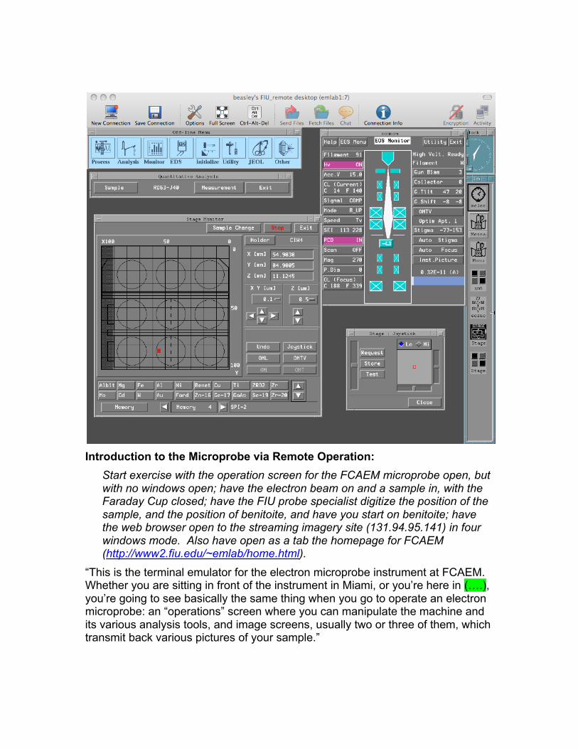
Introduction to the Microprobe via Remote Operation:

Start exercise with the operation screen for the FCAEM microprobe open, but with no windows open; have the electron beam on and a sample in, with the Faraday Cup closed; have the FIU probe specialist digitize the position of the sample, and the position of benitoite, and have you start on benitoite; have the web browser open to the streaming imagery site (131.94.95.141) in four windows mode. Also have open as a tab the homepage for FCAEM (http://www2.fiu.edu/~emlab/home.html).

“This is the terminal emulator for the electron microprobe instrument at FCAEM. Whether you are sitting in front of the instrument in Miami, or you’re here in (….), you’re going to see basically the same thing when you go to operate an electron microprobe: an “operations” screen where you can manipulate the machine and its various analysis tools, and image screens, usually two or three of them, which transmit back various pictures of your sample.”

• Open the EPMA Menu on the operations screen (mouseclick on blank screen for function list: pick EPMA MENU); a functions bar will appear, along with a active functions tab on the right side of the screen.

• Under the “Monitor” tab, open EOS Monitor and Stage. The EOS monitor window is a mock-up of the beam path with controls for various microprobe functions; The Stage monitor is a mock-up of the microprobe stage that provides X-Y-Z coordinates for your location and that of samples and standards

• Under the Analysis tab, click Quantitative Analysis. The Quantitative Analysis menu appears.

• On the Stage window, click Joystick, and move the Joystick window to a clear space on the emulator screen.

Arrange these windows once they appear so that you have a clear view of each one, ideally without tiling them – this will take up most of the screen.

“This is a JEOL 8900R Superprobe, with five WDS spectrometers, and an EDS spectrometer (and I’m sure you all know exactly what that means right now!) Let’s take a little tour of the probe’s operation system. If you want to see a picture of the instrument itself, you can bounce to the FCAEM site.”

Choose the FIU-FCAEM tab on the web browser; click Instrumentation/EPMA on the menu. After pointing it out, and the address for students on their PC’s, tab back to the images window.

“The instrument is at its core an electron gun, represented symbolically here in the EOS Monitor window. You have a tungsten filament at the top of the flight tube (think: like a big incandescent light bulb!) which is heated to produce electrons. The electrons are moved at high velocity toward the sample due to a high potential gradient – typically for our uses about 15 KV. However, the current itself is really low: not more than 20 nanoamps when you’re doing measurements. With such a small current it’s important that nothing get in the way of the electrons, so the whole flight tube is kept at very high vacuum. “The electron beam is focused using electrostatic lenses down to a very small diameter: usually only a couple of micrometers across. One thing that is important to do is figure out where the electron beam is – the tuning and focusing is fussy enough that it’s never perfectly centered. What we do to find the “spot” is we place the mineral benitoite under the beam. Benitoite fluoresces when hit by the beam, so we can see the position and size of our “spot” when we go to measure things on our sample.”

• Open the Faraday cup by clicking on it in EOS Monitor; a bright blue/lavender spot should appear on the upper right window in the image screen; if not, check EOS Monitor and make sure SCAN is off.

• Now click OMTV on the EOS Monitor screen: the reflected light image of the sample should appear with the spot still evident. If it doesn’t flash up on its own, refresh the window on the web browser.

“So, the “spot” is (…almost always somewhere other than) at the crosshairs on our sample. The image we’re looking at here is a reflected light microscope image – the microprobe includes a basic reflected light scope, with a set magnification of 400x (How does this compare to the magnifications you use on your petrographic microscopes?.....). Note how surface roughness is really evident in the reflected light image – we’ll be using that to find good spots to analyze, as we want those places to be as flat and “shiny” as we can find. “Now to actually find and measure things on the microprobe we need better and more flexible imagery than this. Fortunately, we have the ability to image the sample in a couple different ways. I’m going to move us over to our test sample now, and we’ll see how the other imagery works.”

Talk through this as you do it - • On the Quantitative Analysis window, pick your sample:

• under Sample, pick Group; • under Group, pick your group (folder of sample data and functions),

then choose your sample from the list. • On the Quantitative Analysis window, hit Measurement/Stage

Condition. A new window will appear listing digitized positions on the sample – usually only one for new samples.

• Select the position, then hit Position Input – a large new window appears including an image of the stage identifying the position of the point.

• To the right of this image, hit Move to move to the chosen spot on your sample.

• On the EOS Monitor, turn OMTV off and SCAN on; an image of some sort should appear on the upper left window on the images screen, either a Secondary Electron (SEI) or electron backscatter (COMP) image.

“The picture you’re seeing now is generated from the incident electrons on the sample. We’re in SCAN mode, which means the electron beam is diffused and rastered so as to cover a larger area. When we turn SCAN off, we go to single point mode – here the beam is at its smallest diameter (and therefore highest intensity on the sample it’s hitting), and it’s in this mode we do measurements. “We typically look at two different images: a Secondary Electron image (SEI mode on the JEOL probe), which is generated in response to the incident electron beam; and an Electron Backscatter image (or COMP mode), which is an imaging approach related to the early experiments by Ernest Rutherford, where he documented the presence of “nuclei” in gold foil. The backscatter response is correlated directly to the average size of the nuclei in the materials being hit with the electron beam, so the backscatter gets “brighter” as a function of the mean atomic number of the minerals. That is to say, minerals that have high Z atoms in them – like zirconium in zircon, cerium in monazite, or more commonly iron and titanium bearing minerals – will look brighter in backscatter mode than minerals comprised of low Z atoms. We can toggle from SEI to COMP mode under SCAN on the EOS Monitor screen.”

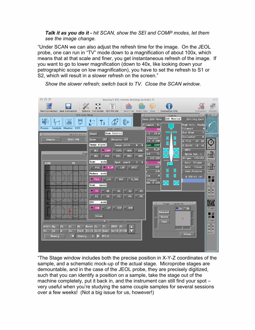
Talk it as you do it - hit SCAN, show the SEI and COMP modes, let them see the image change.

“Under SCAN we can also adjust the refresh time for the image. On the JEOL probe, one can run in “TV” mode down to a magnification of about 100x, which means that at that scale and finer, you get instantaneous refresh of the image. If you want to go to lower magnification (down to 40x, like looking down your petrographic scope on low magnification), you have to set the refresh to S1 or S2, which will result in a slower refresh on the screen.”

Show the slower refresh; switch back to TV. Close the SCAN window.

“The Stage window includes both the precise position in X-Y-Z coordinates of the sample, and a schematic mock-up of the actual stage. Microprobe stages are demountable, and in the case of the JEOL probe, they are precisely digitized, such that you can identify a position on a sample, take the stage out of the machine completely, put it back in, and the instrument can still find your spot – very useful when you’re studying the same couple samples for several sessions over a few weeks! (Not a big issue for us, however!)

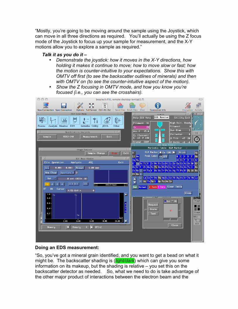
“Mostly, you’re going to be moving around the sample using the Joystick, which can move in all three directions as required. You’ll actually be using the Z focus mode of the Joystick to focus up your sample for measurement, and the X-Y motions allow you to explore a sample as required.”

Talk it as you do it – • Demonstrate the joystick: how it moves in the X-Y directions, how

holding it makes it continue to move; how to move slow or fast; how the motion is counter-intuitive to your expectations. Show this with OMTV off first (to see the backscatter outlines of minerals) and then with OMTV on (to see the counter-intuitive aspect of the motion).

• Show the Z focusing in OMTV mode, and how you know you’re focused (i.e., you can see the crosshairs).

Doing an EDS measurement: “So, you’ve got a mineral grain identified, and you want to get a bead on what it might be. The backscatter shading is (light/dark) which can give you some information on its makeup, but the shading is relative – you set this on the backscatter detector as needed. So, what we need to do is take advantage of the other major product of interactions between the electron beam and the

sample: the emission of X-rays that are characteristic of the elements in the materials analyzed. Electron microprobes have two instruments that do this: a Wavelength Dispersive X-ray Spectrometer (WDS) and an Energy Dispersive X-ray Spectrometer (EDS). For quick-and-dirty non-quantitative examinations, we use the EDS spectrometer.”

Talk it as you do it – • Open up the EDS window by hitting EDS on the EMPA Menu and

selecting EDS from the dropdown list, which opens the EDS window, a graphic interface that is basically a plot of energy versus wavelength for the generated X-rays.

“The EDS spectrometer makes use of a particular kind of X-ray detector (called a Silicon Drift detector) that allows it to look at the entire X-ray spectrum simultaneously. What we’ll get back is a scan of all the X ray wavelengths the sample is emitting, and we can then match these to different elements based on their X ray profiles.”

Talk it as you do it: do an EDS measurement of the mineral under the beam!

• Turn SCAN off on the EOS monitor window • Hit ACQ on the EDS window; let it run for a few seconds to generate

the scan.

“Now that we have X-ray peaks, how do we tell what is what?” Talk it as you do it –

• Open Periodic Table on the EDS window: the periodic table appears. • Pick several elements in the low Z range to see where their peaks are;

iteratively match up the peaks with the right elements. • Identify with the class the elements that are in the mineral being

analyzed. “Note that the program identifies different kinds of X-ray peaks for different elements: for low Z elements (most of the common ones) we get Kα peaks; but for some of the heavier elements (Zr, Ce, Th, etc), we see Lα peaks. What the program is doing is picking based on the most intense X-ray peaks for each element. Note also that on the EDS spectrometer, there is not a simple relationship between peak height and concentration: in fact, as Z goes up, the peak intensity at a given concentration level of an element goes down, and this trend is distinct for the Kα, Kβ, and Lα peaks. So the EDS spectrometer can really only be used as a chemical identification tool of sorts: it can tell you what elements are in the sample, but it can’t quantify them. For that we need a different spectrometer.” Using the Wavelength Dispersive Spectrometer: “The Wavelength Dispersive Spectrometer works on the principle of X-ray diffraction: X-rays entering the spectrometer hit an analyzing crystal, which then diffracts a small subset of them, representing a particular element, at a particular angle of diffraction into a Faraday Cup detector.”

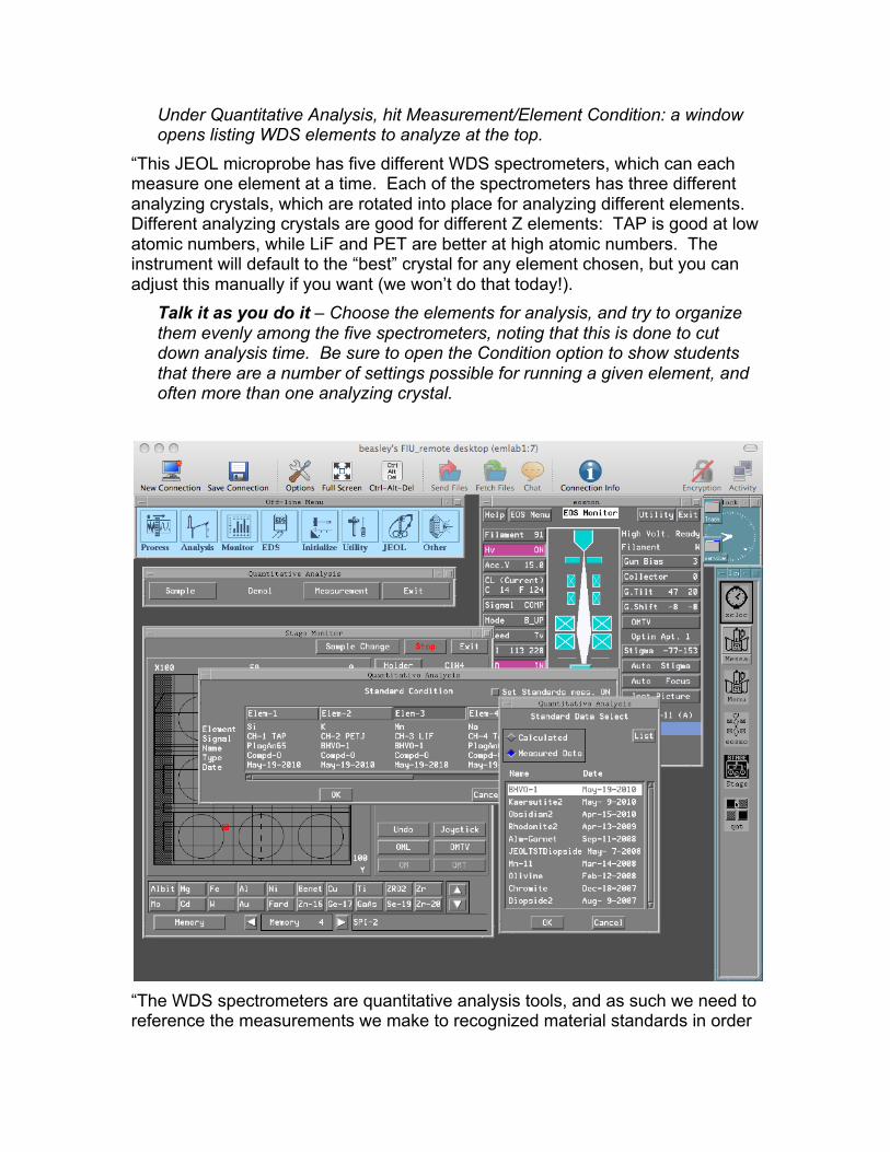
Under Quantitative Analysis, hit Measurement/Element Condition: a window opens listing WDS elements to analyze at the top.

“This JEOL microprobe has five different WDS spectrometers, which can each measure one element at a time. Each of the spectrometers has three different analyzing crystals, which are rotated into place for analyzing different elements. Different analyzing crystals are good for different Z elements: TAP is good at low atomic numbers, while LiF and PET are better at high atomic numbers. The instrument will default to the “best” crystal for any element chosen, but you can adjust this manually if you want (we won’t do that today!).

Talk it as you do it – Choose the elements for analysis, and try to organize them evenly among the five spectrometers, noting that this is done to cut down analysis time. Be sure to open the Condition option to show students that there are a number of settings possible for running a given element, and often more than one analyzing crystal.

“The WDS spectrometers are quantitative analysis tools, and as such we need to reference the measurements we make to recognized material standards in order

to calibrate the spectrometer signals. So, we need to choose an appropriate mineral standard for each element we’re analyzing by WDS.”

Talk it as you do it - Close Element condition, and open Standard Condition on the Measurement drop-down. A list of elements will appear, with a default standard (usually what was run for that element in the last run, whatever that might have been). Click on the header for an element to open the list of possible standards – this is a new, small window that lists all the available standard data for each element and the dates each standard was run.

“The microprobe has a data correction and calibration system called the ZAF system: Z (for atomic number effects – X-ray intensities decline with increasing atomic number), A (for absorbence – some emitted X-rays are absorbed by the materials being hit with the beam), and F (for Fluorescence: some materials emit secondary X-rays related to the primary X-rays passing through them (remember what happens when you put iron-rich samples in an XRD?)). The calibration protocol is complicated and (fortunately) automated, but it depends critically on a good choice of standards. The rule of thumb when doing microprobe standardization is: compare apples to apples whenever possible. So, if we know we have feldspars in our rock, we make sure to use feldspar standards for Si, Al, Ca, Na, and even K; same for pyroxene, olivine, garnet, etc. The problem is that you can’t easily do this for every element in every mineral – ultimately you have to make some compromises (like for example, running Si in all the minerals off of a feldspar standard, Ca off a pyroxene standard, Al off of feldspar, etc.) The challenge is getting the best set of standard choices, which can be difficult for challenging samples.”

Talk it as you do it – Change a couple standards for a few elements to more recent and/or better fit standards.

“When you’re choosing standards, aside from trying to fit them mineralogically to what you’re likely to see in your sample, you also want to choose the most recent data possible, to be sure that the intensity-to-concentration relationship for the standard is likely to be the same as what you’ll find in your unknowns. The beauty of the JEOL microprobe is that the sensitivity of the instrument (that is, the magnitude of signal you get per unit concentration) is very robust over time, so we can use standards data successfully even if it is a month or more old. “So, now that we have standards we like for the run, we should try measuring something!”

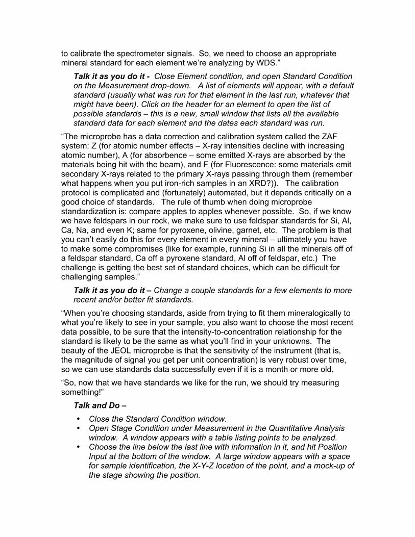
Talk and Do – • Close the Standard Condition window. • Open Stage Condition under Measurement in the Quantitative Analysis

window. A window appears with a table listing points to be analyzed. • Choose the line below the last line with information in it, and hit Position

Input at the bottom of the window. A large window appears with a space for sample identification, the X-Y-Z location of the point, and a mock-up of the stage showing the position.

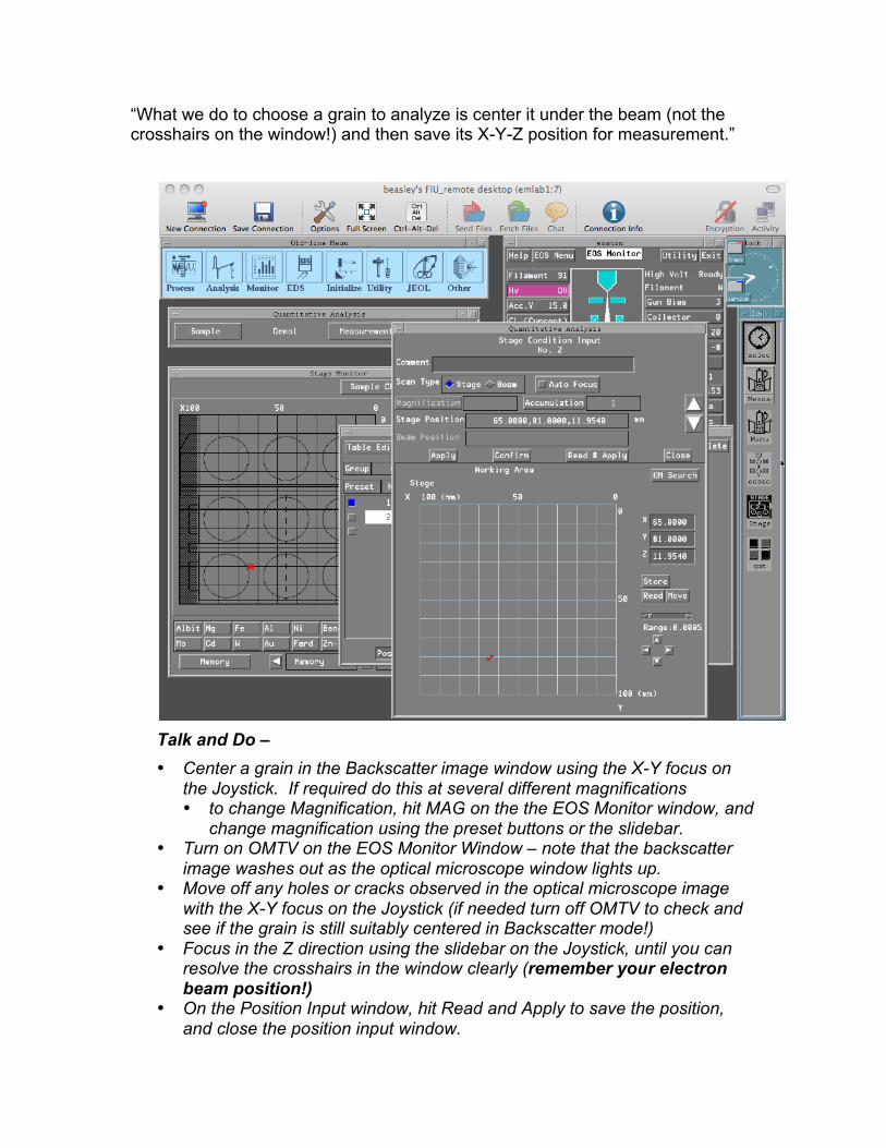
“What we do to choose a grain to analyze is center it under the beam (not the crosshairs on the window!) and then save its X-Y-Z position for measurement.”

Talk and Do – • Center a grain in the Backscatter image window using the X-Y focus on

the Joystick. If required do this at several different magnifications • to change Magnification, hit MAG on the the EOS Monitor window, and

change magnification using the preset buttons or the slidebar. • Turn on OMTV on the EOS Monitor Window – note that the backscatter

image washes out as the optical microscope window lights up. • Move off any holes or cracks observed in the optical microscope image

with the X-Y focus on the Joystick (if needed turn off OMTV to check and see if the grain is still suitably centered in Backscatter mode!)

• Focus in the Z direction using the slidebar on the Joystick, until you can resolve the crosshairs in the window clearly (remember your electron beam position!)

• On the Position Input window, hit Read and Apply to save the position, and close the position input window.

Repeat this procedure several times to digitize 3-4 points on grains with different backscatter brightnesses. Then close the Stage Condition window.

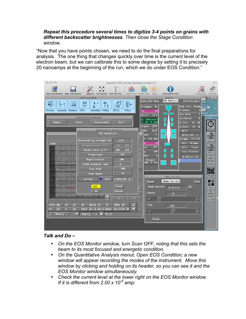
“Now that you have points chosen, we need to do the final preparations for analysis. The one thing that changes quickly over time is the current level of the electron beam, but we can calibrate this to some degree by setting it to precisely 20 nanoamps at the beginning of the run, which we do under EOS Condition.”

Talk and Do –

• On the EOS Monitor window, turn Scan OFF, noting that this sets the beam to its most focused and energetic condition.

• On the Quantitative Analysis menut, Open EOS Condition; a new window will appear recording the modes of the instrument. Move this window by clicking and holding on its header, so you can see it and the EOS Monitor window simultaneously.

• Check the current level at the lower right on the EOS Monitor window. If it is different from 2.00 x 10-8 amp:

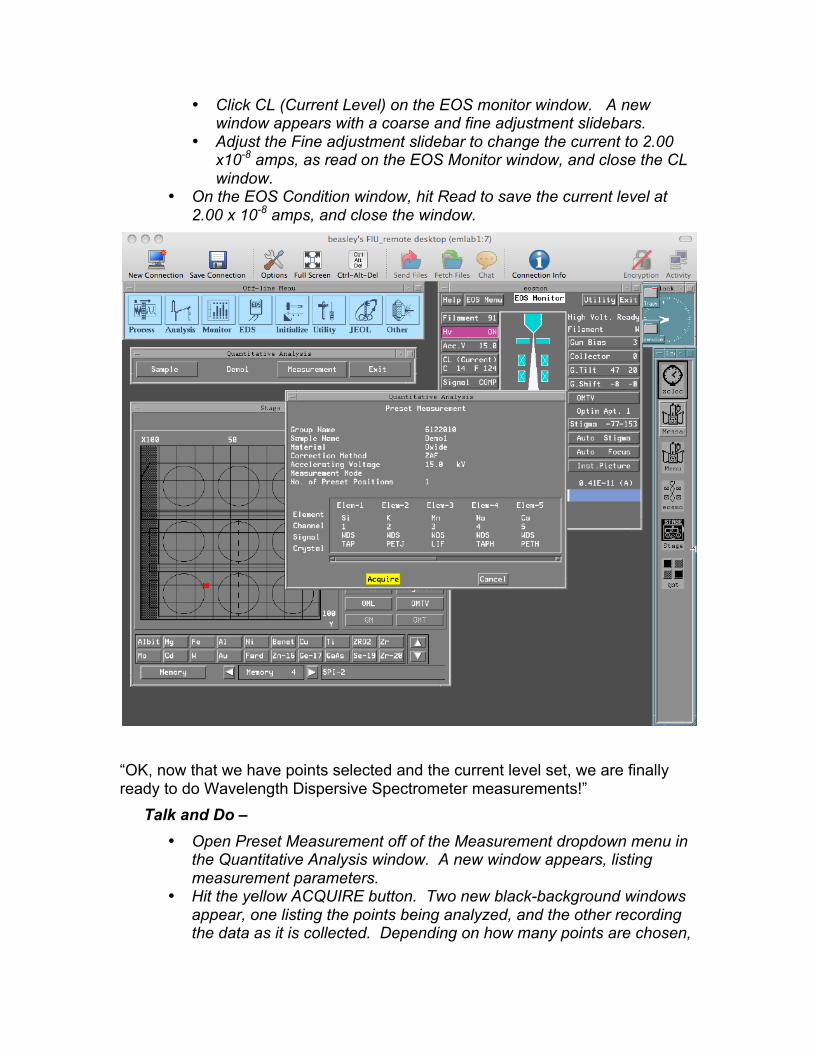
• Click CL (Current Level) on the EOS monitor window. A new window appears with a coarse and fine adjustment slidebars.

• Adjust the Fine adjustment slidebar to change the current to 2.00 x10-8 amps, as read on the EOS Monitor window, and close the CL window.

• On the EOS Condition window, hit Read to save the current level at 2.00 x 10-8 amps, and close the window.

“OK, now that we have points selected and the current level set, we are finally ready to do Wavelength Dispersive Spectrometer measurements!”

Talk and Do – • Open Preset Measurement off of the Measurement dropdown menu in

the Quantitative Analysis window. A new window appears, listing measurement parameters.

• Hit the yellow ACQUIRE button. Two new black-background windows appear, one listing the points being analyzed, and the other recording the data as it is collected. Depending on how many points are chosen,

this may take 5-10 minutes. When data collection is completed, you’ll see MEASUREMENT END in small print in the left-hand analysis window. Usually the elemental readout from the last analysis will also appear here.

• An option: on the Web browser, open MINDAT.org or a like listing of common minerals, and have students try and determine what minerals have just been analyzed based on their oxide analyses on the microprobe. In my course, I refer them back to an exercise I give at the beginning of the term, where I require them to calculate mineral formulas from oxide weight percents.

Repeat the procedure of selecting a grain to analyze, conducting an EDS measurement on the grain, and then digitizing and analyzing it via WDS analysis a couple times, to get the class familiar with the procedure. At this point (time permitting) I recommend letting students in the class direct you to analyze different things they see in the images of the sample – you’re the “driver”, and they tell you precisely what to do to center the sample and make the measurement. This works best if the sample you’re using is one the students have some feeling of ownership over – a sample collected on a class field trip, or the focus of a class lab exercise or project. In this “class driving” activity, it’s important that you do exactly what the students tell you to in terms of every step of picking points and doing the measurements, even if that direction is mistaken (I do what they say, then ask if that’s right, and let other students correct my actions). This helps students recognize the problem places in doing the procedures for analyzing samples, and (important!) it demonstrates to them that making these kinds of mistakes are not dangerous to the machine or their work – they just have to stop and do it over correctly, and it’s easy to do so. I’ll often do this for an hour, or until students stop being responsive. Usually one or two students will want to do some analyses themselves, which I allow. Optional: Generating text files of microprobe results for data download:

• From the EPMA Menu, choose Process. The Process menu appears. • Select Quantitative Analysis from the Process menu. A small window

appears, with a couple option buttons. • Choose Summary. The Summary menu appears. • Ensure that the sample listed in the menu is the one you wish to compile

data for. If not: • Choose Sample. A window appears identifying Groups (folders) and

samples in that Group.

• Choose Group (a pull-down menu of Group folders appears) select your group, and close the menu. If a message appears asking if you want to keep the measurement conditions, select Yes.

• The samples in your Group should now be listed in the Sample window. Choose your sample (say Yes to the measurement condition message if it appears) and close the window.

• Select Summary from the Summary menu. Three options appear; choose Summary again. A window appears that includes a listing for all points analyzed for your sample, and two sets of command buttons for different data reporting options. I typically choose Oxide wt. % in the top set, and Spreadsheet in the bottom one, but you can tailor the data report to your needs.

• At the bottom of the window, choose Type Out. A black-background window appears in which your sample data is tabulated.

• At the top of the window, select Save. A small window appears listing the directory, menu, and file of the saved file – the name of the file is always Summary.tx, which is a default. I recommend changing the filename to a more recognizable title.

• Select OK on this window to save the file, and close all the windows.