Score Function for Data MiningAlgorithms

Chapter 7 of HTF

David Madigan

Algorithm Components1. The task the algorithm is used to address (e.g.classification, clustering, etc.)

2. The structure of the model or pattern we are fitting to thedata (e.g. a linear regression model)

3. The score function used to judge the quality of the fittedmodels or patterns (e.g. accuracy, BIC, etc.)

4. The search or optimization method used to search overparameters and/or structures (e.g. steepest descent,MCMC, etc.)

5. The data management technique used for storing, indexing,and retrieving data (critical when data too large to reside inmemory)

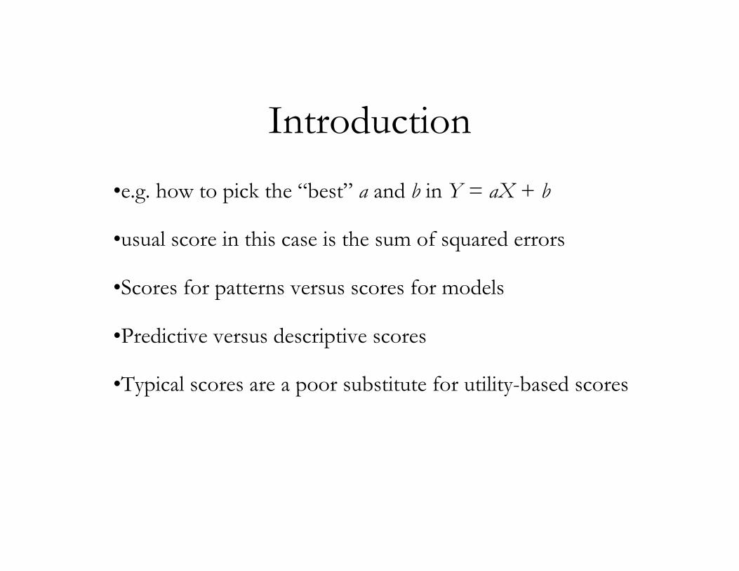
Introduction

•e.g. how to pick the “best” a and b in Y = aX + b

•usual score in this case is the sum of squared errors

•Scores for patterns versus scores for models

•Predictive versus descriptive scores

•Typical scores are a poor substitute for utility-based scores

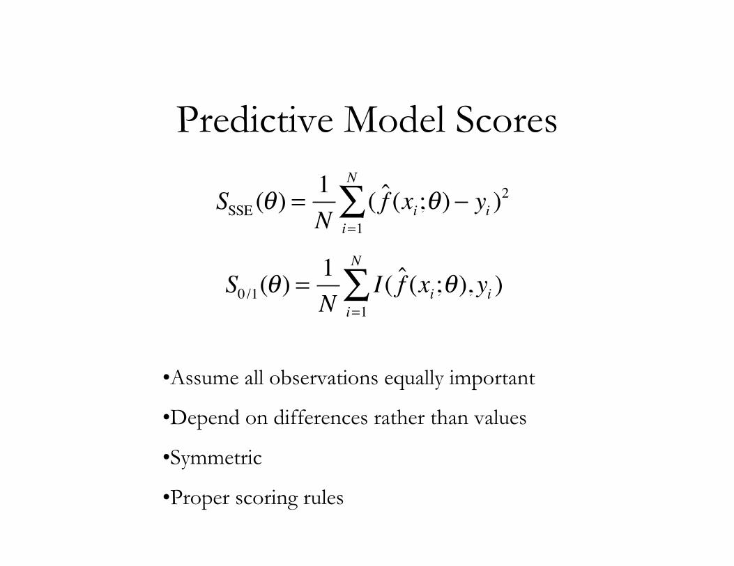
Predictive Model Scores

SSSE(!) =

1

N( f (xi;!) " yi )

2

i=1

N

#

S0 /1(!) =

1

NI( f (xi;!), yi )

i=1

N

"

•Assume all observations equally important

•Depend on differences rather than values

•Symmetric

•Proper scoring rules

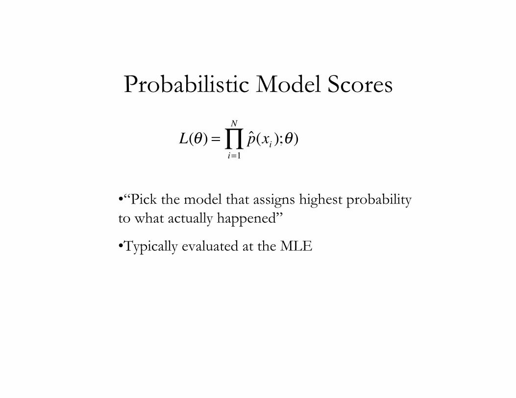
Probabilistic Model Scores

L(!) = p(xi);!)

i=1

N

"

•“Pick the model that assigns highest probabilityto what actually happened”

•Typically evaluated at the MLE

Optimism of the Training Error Rate•Typically the training error rate:

is an optimistically biased estimate of the true error rate:

err =1

NL(yi , f (xi )

i=1

N

!

EX ,y L(yi , f (xi )!"

#$

"in-sample" error

•Consider the error rate with fixed x's

•Can show squared-error, 0-1, and other loss functions:

•For the standard linear model with p predictors:

Errin=1

NE yEY

new L(Yinew, f (xi )

i=1

N

!

Errin! E y (err) =

2

NCov(yi , yi )

i=1

N

"

Errin

= Ey(err) + 2

p

N!

"

2

Cp and AIC

•Leads directly to the Cp statistic for scoring models

•The Akaike Information Criterion (AIC) is derived simialrly

but applies more generally to log likelihood loss

where loglik is the maximized log likelihood. AIC coincides

with Cp for the linear model

Cp= err + 2p

N!

"

2

AIC= -2

N! loglik + 2

p

N

Selects overly complex models?

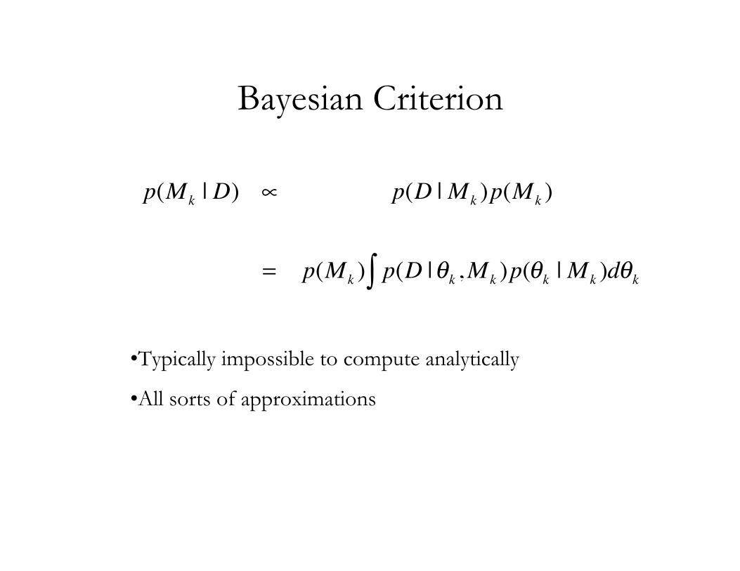
Bayesian Criterion

p(Mk | D) ! p(D |Mk )p(Mk )

= p(Mk ) p(D |"k ,Mk )p("k |Mk )d"k#

•Typically impossible to compute analytically

•All sorts of approximations

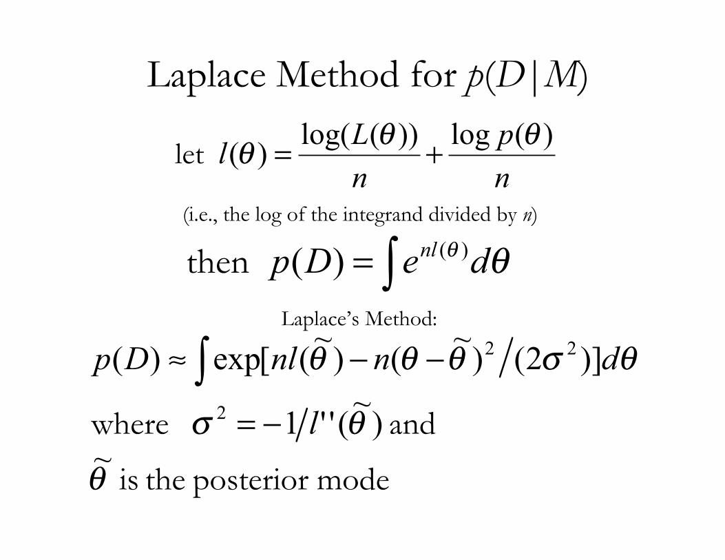
Laplace Method for p(D|M)

n

p

n

Ll

)(log))(log()(

!!! +=let

(i.e., the log of the integrand divided by n)

!= "" deDp nl )()( then

Laplace’s Method:

modeposterior the is

and where

!

!"

!"!!!

~)~(''1

)]2()~

()~([exp)(

2

22

l

dnnlDp

#=

##$ %

Laplace cont.

)}~(exp{2

)]2()~

()~([exp)(

21

22

!"#

!"!!!

nln

dnnlDp

$%

$$= &

•Tierney & Kadane (1986, JASA) show the approximation is O(n-1)

•Using the MLE instead of the posterior mode is also O(n-1)

•Using the expected information matrix in σ is O(n-1/2) butconvenient since often computed by standard software

•Raftery (1993) suggested approximating by a single Newton stepstarting at the MLE

•Note the prior is explicit in these approximations

!~

Monte Carlo Estimates of p(D|M)

!= """ dpDpDp )()|()(

Draw iid θ1,…, θm from p(θ):

!=

=

m

i

iDp

mDp

1

)( )|(1

)(ˆ "

In practice has large variance

Monte Carlo Estimates of p(D|M) (cont.)

Draw iid θ1,…, θm from p(θ|D):

!

!

=

==

m

i

i

m

i

i

i

w

Dpwm

Dp

1

1

)( )|(1

)(ˆ

"

)()|(

)()(

)|(

)()()(

)(

)(

)(

ii

i

i

i

ipDp

Dpp

Dp

pw

!!

!

!

!==

“ImportanceSampling”

Monte Carlo Estimates of p(D|M) (cont.)

1

1

1)(

1)(

1

)(

)(

)|(1

)|(

)(

)|()|(

)(1

)(ˆ

!

=

!

=

=

"#$

%&'

=

=

(

(

(

m

i

i

m

ii

m

i

i

i

Dpm

Dp

Dp

DpDp

Dp

mDp

)

)

))

Newton and Raftery’s “Harmonic Mean Estimator”

Unstable in practice and needs modification

p(D|M) from Gibbs Sampler Output

)|(

)()|()(

*

**

Dp

pDpDp

!

!!=

Suppose we decompose θ into (θ1,θ2) such that p(θ1|D,θ2) and p(θ2|D,θ1) are available in closed-form…

First note the following identity (for any θ* ):

Chib (1995)

p(D|θ*) and p(θ*) are usually easy to evaluate.

What about p(θ*|D)?

p(D|M) from Gibbs Sampler Output

The Gibbs sampler gives (dependent) draws fromp(θ1, θ2 |D) and hence marginally from p(θ2 |D)…

)|(),|()|,( *

1

*

1

*

2

*

2

*

1 DpDpDp !!!!! =

222

*

1

*

1 )|(),|()|( !!!!! dDpDpDp "=

!=

"G

g

gDp

G 1

)(

2

*

1 ),|(1

##

What about 3 parameter blocks…

To get these draws, continue the Gibbs sampler sampling in turn from:

)|(),|(),,|()|,,( *

1

*

1

*

2

*

2

*

1

*

3

*

3

*

2

*

1 DpDpDpDp !!!!!!!!! =

3

*

133

*

1

*

2

*

1

*

2 ),|(),,|(),|( !!!!!!!! dDpDpDp "=

!=

"G

g

gDp

G 1

)(

3

*

1

*

2 ),,|(1

###

OK OK?

),,|( 3

*

12 !!! Dp and ),,|( 2

*

13 !!! Dp

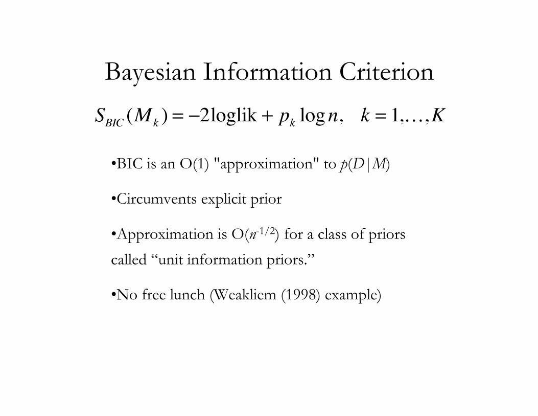
Bayesian Information Criterion

SBIC (Mk ) = !2loglik + pk logn, k = 1,…,K

•BIC is an O(1) "approximation" to p(D|M)

•Circumvents explicit prior

•Approximation is O(n-1/2) for a class of priors

called “unit information priors.”

•No free lunch (Weakliem (1998) example)