SCOPE: parallel databases meet MapReducejrzhou/pub/Scope-VLDBJ.pdfSCOPE: parallel databases meet...

The VLDB JournalDOI 10.1007/s00778-012-0280-z

SPECIAL ISSUE PAPER

SCOPE: parallel databases meet MapReduce

Jingren Zhou · Nicolas Bruno · Ming-Chuan Wu ·Per-Ake Larson · Ronnie Chaiken · Darren Shakib

Received: 15 August 2011 / Revised: 16 February 2012 / Accepted: 14 May 2012© Springer-Verlag 2012

Abstract Companies providing cloud-scale data serviceshave increasing needs to store and analyze massive data sets,such as search logs, click streams, and web graph data. Forcost and performance reasons, processing is typically done onlarge clusters of tens of thousands of commodity machines.Such massive data analysis on large clusters presents newopportunities and challenges for developing a highly scal-able and efficient distributed computation system that iseasy to program and supports complex system optimizationto maximize performance and reliability. In this paper, wedescribe a distributed computation system, Structured Com-putations Optimized for Parallel Execution (Scope), targetedfor this type of massive data analysis. Scope combines bene-fits from both traditional parallel databases and MapReduceexecution engines to allow easy programmability and delivermassive scalability and high performance through advancedoptimization. Similar to parallel databases, the system has aSQL-like declarative scripting language with no explicit par-allelism, while being amenable to efficient parallel executionon large clusters. An optimizer is responsible for convert-ing scripts into efficient execution plans for the distributed

J. Zhou (B) · N. Bruno · M.-C. Wu · P.-A. Larson ·R. Chaiken · D. ShakibMicrosoft Corp., One Microsoft Way, Redmond, WA 98052, USAe-mail: [email protected]

N. Brunoe-mail: [email protected]

M.-C. Wue-mail: [email protected]

P.-A. Larsone-mail: [email protected]

R. Chaikene-mail: [email protected]

D. Shakibe-mail: [email protected]

computation engine. A physical execution plan consists of adirected acyclic graph of vertices. Execution of the plan isorchestrated by a job manager that schedules execution onavailable machines and provides fault tolerance and recovery,much like MapReduce systems. Scope is being used dailyfor a variety of data analysis and data mining applicationsover tens of thousands of machines at Microsoft, poweringBing, and other online services.

Keywords SCOPE · Parallel databases · MapReduce ·Distributed computation · Query optimization

1 Introduction

The last decade witnessed an explosion in the volumes ofdata being stored and processed. More and more companiesrely on the results of such massive data analysis for their busi-ness decisions. Web companies, in particular, have increas-ing needs to store and analyze the ever growing data, such assearch logs, crawled web content, and click streams, usuallyin the range of petabytes, collected from a variety of webservices. Such analysis is becoming crucial for businesses ina variety of ways, such as to improve service quality and sup-port novel features, to detect changes in patterns over time,and to detect fraudulent activities.

One way to deal with such massive amounts of data is torely on a parallel database system. This approach has beenextensively studied for decades, incorporates well-knowntechniques developed and refined over time, and mature sys-tem implementations are offered by several vendors. Paralleldatabase systems feature data modeling using well-definedschemas, declarative query languages with high levels ofabstraction, sophisticated query optimizers, and a rich run-time environment that supports efficient execution strategies.

123

J. Zhou et al.

At the same time, database systems typically run only onexpensive high-end servers. When the data volumes to bestored and processed reaches a point where clusters of hun-dreds or thousands of machines are required, parallel data-base solutions become prohibitively expensive. Worse still,at such scale, many of the underlying assumptions of par-allel database systems (e.g., fault tolerance) begin to breakdown, and the classical solutions are no longer viable with-out substantial extensions. Additionally, web data sets areusually non-relational or less structured and processing suchsemi-structured data sets at scale poses another challenge fordatabase solutions.

To be able to perform the kind of data analysis describedabove in a cost-effective manner, several companies havedeveloped distributed data storage and processing sys-tems on large clusters of low-cost commodity machines.Examples of such initiatives include Google’s MapRe-duce [11], Hadoop [3] from the open-source community, andCosmos [7] and Dryad [31] at Microsoft. These systems aredesigned to run on clusters of hundreds to tens of thousandsof commodity machines connected via a high-bandwidth net-work and expose a programming model that abstracts distrib-uted group-by-aggregation operations.

In the MapReduce approach, programmers provide mapfunctions that perform grouping and reduce functions thatperform aggregation. These functions are written in proce-dural languages like C++ and are therefore very flexible. Theunderlying runtime system achieves parallelism by partition-ing the data and processing different partitions concurrently.

This model scales very well to massive data sets and hassophisticated mechanisms to achieve load-balancing, outlierdetection, and recovery to failures, among others. However,it also has several limitations. Users are forced to trans-late their business logic to the MapReduce model in orderto achieve parallelism. For some applications, this map-ping is very unnatural. Users have to provide implemen-tations for the map and reduce functions, even for simpleoperations like projection and selection. Such custom codeis error-prone and difficult to reuse. Moreover, for appli-cations that require multiple stages of MapReduce, thereare often many valid evaluation strategies and executionorders. Having users implement (potentially multiple) mapand reduce functions is equivalent to asking users to spec-ify physical execution plans directly in relational databasesystems, an approach that became obsolete with the intro-duction of the relational model over three decades ago.Hand-crafted execution plans are more often than not subop-timal and may lead to performance degradation by orders ofmagnitude if the underlying data or configurations change.Moreover, attempts to optimize long MapReduce jobs arevery difficult, since it is virtually impossible to do com-plex reasoning over sequences of opaque MapReduce oper-ations.

Recent work has systematically compared parallel dat-abases and MapReduce systems, and identified their strengthsand weaknesses [27]. There has been a flurry of workto address various limitations. High-level declarative lan-guages, such as Pig [23], Hive [28,29], and Jaql [5], weredeveloped to allow developers to program at a higher levelof abstraction. Other runtime platforms, including Nep-hele/PACTs [4] and Hyracks [6], have been developed toimprove the MapReduce execution model.

In this paper, we describe Scope (Structured Computa-tions Optimized for Parallel Execution) our solution thatincorporates the best characteristics of both parallel dat-abases and MapReduce systems. Scope [7,32] is the com-putation platform for Microsoft online services targeted forlarge-scale data analysis. It executes tens of thousands ofjobs daily and is well on the way to becoming an exabytecomputation platform.

In contrast to existing systems, Scope systematicallyleverages technology from both parallel databases andMapReduce systems throughout the software stack. TheScope language is declarative and intentionally reminis-cent of SQL, similar to Hive [28,29]. The select statementis retained along with joins variants, aggregation, and setoperators. Users familiar with SQL thus require little or notraining to use Scope. Like SQL, data are internally mod-eled as sets of rows composed of typed columns and everyrow set has a well-defined schema. This approach makesit possible to store tables with schemas defined at designtime and to create and leverage indexes during execution.At the same time, the language is highly extensible and isdeeply integrated with the .NET framework. Users can easilydefine their own functions and implement their own versionsof relational operators: extractors (parsing and constructingrows from a data source, regardless of whether it is struc-tured or not), processors (row-wise processing), reducers(group-wise processing), combiners (combining rows fromtwo inputs), and outputters (formatting and outputting finalresults). This flexibility allows users to process both rela-tional and non-relational data sets and solves problems thatcannot be easily expressed in traditional SQL, while at thesame time retaining the ability to perform sophisticated opti-mization of user scripts.

Scope includes a cost-based optimizer based on theCascades framework [15] that generates efficient execu-tion plans for given input scripts. Since the language isheavily influenced by SQL, Scope is able to leverageexisting work on relational query optimization and per-form rich and non-trivial query rewritings that considerthe input script as a whole. The Scope optimizer extendsthe original Cascades framework by incorporating uniquerequirements derived from the context of distributed queryprocessing. In particular, parallel plan optimization is fullyintegrated into the optimizer, instead of being done at the

123


post-optimization phase. The property framework is alsoextended to reason about more complex structural data prop-erties.

The Scope runtime provides implementations of manystandard physical operators, saving users from having imple-menting similar functionality repeatedly. Moreover, differentimplementation flavors of a given physical operator providethe optimizer a rich search space to find an efficient execu-tion plan. At a high level, a script is compiled into units ofexecution and data flow relationships among such units. Thisexecution graph relies on a job manager to schedule work todifferent machines for execution and to provide fault toler-ance and recovery, like in MapReduce systems. Each sched-uled unit, in turn, can be seen as an independent executionplan and is executed in a runtime environment that borrowsideas from traditional database systems.

The rest of this paper is structured as follows. In Sect. 2,we give a high-level overview of the distributed data plat-form that supports Scope. In Sect. 3, we explain how dataare modeled and stored in the system. In Sect. 4, we introducethe Scope language. In Sect. 5, we describe in considerabledetail the compilation and optimization of Scope scripts. InSect. 6, we introduce the code generation and runtime sub-systems, and in Sect. 7, we explain how compiled scriptsare scheduled and executed in the cluster. We present a casestudy in Sect. 8. Finally, we review related work in Sect. 9and conclude in Sect. 10.

2 Platform architecture

Scope relies on a distributed data platform, named Cos-mos [7], for storing and analyzing massive data sets. Cos-mos is designed to run on large clusters consisting of tensof thousands of commodity servers and has similar goals toother distributed storage systems [3,13]. Disk storage is dis-tributed with each server having one or more direct-attacheddisks. High-level design objectives for the Cosmos platforminclude:

Availability: Cosmos is resilient to hardware failures toavoid whole system outages. Data is replicated throughoutthe system and metadata is managed by a quorum groupof servers to tolerate failures.Reliability: Cosmos recognizes transient hardware condi-tions to avoid corrupting the system. System componentsare checksummed end-to-end and the on-disk data is peri-odically scrubbed to detect corrupt or bit rot data before itis used by the system.Scalability: Cosmos is designed from the ground up tostore and process petabytes of data, and resources are eas-ily increased by adding more servers.Performance: Data is distributed among tens of thou-sands of servers. A job is broken down into small units

Fig. 1 Architecture of the cosmos platform

of computation and distributed across a large number ofCPUs and storage devices.Cost: Cosmos is cheaper to build, operate and expand,per gigabyte, than traditional approaches that use smallernumber of expensive large-scale servers.

Figure 1 shows the architecture of the Cosmos platform.We next describe the main components:

Storage system The storage system is an append-only filesystem optimized for large sequential I/O. All writes areappend-only, and concurrent writers are serialized by the sys-tem. Data are distributed and replicated for fault toleranceand compressed to save storage and increase I/O through-put. The storage system provides a directory with a hier-archical namespace and stores sequential files of unlimitedsize. A file is physically composed of a sequence of extents.Extents are the unit of space allocation and replication. Theyare typically a few hundred megabytes in size. Each com-putation unit generally consumes a small number of col-located extents. Extents are replicated for reliability andalso regularly scrubbed to protect against bit rot. The datawithin an extent consist of a sequence of append blocks.The block boundaries are defined by application appends.Append blocks are typically a few megabytes in size andcontain a collection of application-defined records. Appendblocks are stored in compressed form with compressionand decompression done transparently at the client side. Asservers are connected via a high-bandwidth network, thestorage system supports both local and remote reads andwrites.

123

J. Zhou et al.

Computation system The Scope computation system con-tains the compiler, the optimizer, the runtime, and the exe-cution environment. A query plan is modeled as a dataflowgraph: a directed acyclic graph (DAG) with vertices repre-senting processes and edges representing data flows. In therest of this paper, we discuss these components in detail.

Frontend services This component provides both interfacesfor job submission and management, for transferring data inand out of Cosmos for interoperability, and for monitoringjob queues, tracking job status and error reporting. Jobs aremanaged in separate queues, each of which is assigned to adifferent team with different resource allocations.

3 Data representation

Scope supports processing data files in both unstructured andstructured formats. We call them unstructured streams andstructured streams, respectively.1

3.1 Unstructured streams

Data from the web, such as search logs and click streams, areby nature semi-structured or even unstructured. An unstruc-tured stream is logically a sequence of bytes that is interpretedand understood by users by means of extractors. Extrac-tors must specify the schema of the resulting tuples (whichallows the Scope compiler to bind the schema informationto the relational abstract syntax tree) and implement the iter-ator interface for extracting the data. Analogously, output ofscripts (which are rows with a given schema) can be written tounstructured streams by means of outputters. Both extractorsand outputters are provided by the system for common sce-narios and can be supplied by users for specialized situations.Unlike traditional databases, data can be consumed withoutan explicit and expensive data loading process. Scope pro-vides great flexibility to deal with data sources in a varietyof formats.

3.2 Structured streams

Structured data can be efficiently stored as structured streams.Like tables in databases, a structured stream has a well-defined schema that every record follows. Scope providesan built-in format to store records with different schemas,which allows constant-time access to any column. A struc-tured stream is self-contained and includes, in addition tothe data itself, rich metadata information such as schema,

1 For historical reasons we call data files streams, although they arenot related to the more traditional concept of read-once streams in theliterature.

structural properties (i.e., partitioning and sorting informa-tion), and access methods. This design makes it possible tounderstand structured streams and optimize scripts takingadvantage of their properties without the need of a separatemetadata service.

Partitioning Structured streams can be horizontally parti-tioned into tens of thousands of partitions. Scope supportsa variety of partitioning schemes, including hash and rangepartitioning on a single or composite keys. Based on the datavolume and distribution, Scope can choose the optimal num-ber of partitions and their boundaries by means of samplingand calculating distributed histograms. Data in a partitionare typically processed together (i.e., a partition represents acomputation unit). A partition of a structured stream is com-prised of one or several physical extents. The approach allowsthe system to achieve effective replication and fault recov-ery through extents while providing computation efficiencythrough partitions.

Data affinity A partition can be processed efficiently whenall its extents are stored close to each other. Unlike tradi-tional parallel databases, Scope does not require all extentsof a partition to be stored on a single machine that couldlead to unbalanced storage across machines. Instead, Scopeattempts to store the extents close together by utilizing storeaffinity. Store affinity aims to achieve maximum data local-ity without sacrificing uniform data distribution. Every extenthas an optional affinity id, and all extents with the same affin-ity id belong to an affinity group. The system treats storeaffinity as a placement hint and tries to place all the extentsof an affinity group on the same machine unless the machinehas already been overloaded. In this case, the extents areplaced in the same rack. If the rack is also overloaded, thesystem then tries to place the extents in a close rack based onthe network topology. Each partition of a structured streamis assigned an affinity id. As extents are created within thepartition, they get assigned the same affinity id, so that theyare stored close together.

Stream references The store affinity functionality can alsobe used to associate/affnitize the partitioning of an outputstream with that of a referenced stream. This causes the out-put stream to mirror the partitioning choices (i.e., partitioningfunction and number of partitions) of the referenced stream.Additionally, each partition in the output stream uses theaffinity id of the corresponding partition in the referencedstream. Therefore, two streams that are referenced not onlyare partitioned in the same way, but partitions are physicallyplaced close to each other in the cluster. This layout signifi-cantly improves parallel join performance, as less data neednot be transferred across the network.

123


Indexes for random access Within each partition, a localsort order is maintained through a B-Tree index. This orga-nization not only allows sorted access to the content of apartition, but also enables fast key lookup on a prefix of thesort keys. Such support is very useful for queries that selectonly a small portion of the underlying tables and also formore sophisticated strategies such as index-based joins.

Column groups To address scenarios that require process-ing just a few columns of a wide table, Scope supports thenotion of column groups, which contain vertical partitionsof tables over user-defined subsets of columns. As in theDecomposition Storage Model [9], a record-id field (surro-gate) is added in each column group so that records can bepieced together if needed.

Physical design Partitioning, sorting, column groups, andstream references are useful design choices that enable effi-cient execution plans for certain query classes. As in tradi-tional DBMSs, judicious choices based on query workloadscould improve query performance by orders of magnitudes.Supporting automated physical design tools in Scope is partof our future work.

4 Query language

The Scope scripting language resembles SQL but with inte-grated C# extensions. Its resemblance to SQL reduces thelearning curve for users, eases porting of existing SQL scriptsinto Scope, and allows users to focus on application logicrather than dealing with low-level details of distributed sys-tem. But the integration with C# also allows users to writecustom operators to manipulate row sets where needed. User-defined operators (UDOs) are first-class citizens in Scopeand optimized in the same way as all other system built-inoperators.

A Scope script consists of a sequence of commands,which are data manipulation operators that take one or morerow sets as input, perform some operation on the data, andoutput a row set. Every row set has a well-defined schemathat all its rows must adhere to. Users can name the output ofa command using assignment, and output can be consumedby subsequent commands simply by referring to it by name.Named inputs/outputs enable users to write scripts in multi-ple (small) steps, a style preferred by some programmers.

In the rest of this section, we describe individual compo-nents of the language in more detail.

4.1 Input/output

As explained earlier, Scope supports both unstructured andstructured streams.

Unstructured streams Scope provides two customizablecommands, EXTRACT and OUTPUT, for users to easily readin data from a data source and write out data to a data sink.

Input data to a Scope script are extracted by means ofbuilt-in or user-defined extractors. Scope provides standardextractors such as generic text and commonly used log extrac-tors. The syntax for specifying unstructured inputs is as fol-lows:

EXTRACT <column>[:<type>] {,<column>[:<type>]}FROM <stream_name> {,<stream_name>}USING <extractor> [<args>][WITH SAMPLE(<seed>) <number> PERCENT];

The EXTRACT command extracts data from one or multi-ple data sources, specified in the FROM clause, and outputs asequence of rows with the schema specified in the EXTRACTclause. The optional WITH SAMPLE clause allows users toextract samples from the original input files, which is usefulfor quick experimentation.

Scope outputs data by means of built-in or custom output-ters. The system provides an outputter for text files with cus-tom delimiters and other specialized ones for common tasks.Users can specify expiration dates for streams and thus havesome additional control on storage consumption over time.The syntax of the OUTPUT command is defined as follows:

OUTPUT [<named_rowset>]TO <stream_name>[WITH STREAMEXPIRY <timespan>][USING <outputter_name> [<output_args>]];

Structured streams Users can refer to structured streams asfollows:

SSTREAM <stream_name>;

It is not necessary to specify the columns in structuredstreams as they are retrieved from the stream metadata dur-ing compilation. However, for script readability and main-tainability, columns can be explicitly named:

SELECT a, b, c FROM SSTREAM <stream_name>;

When outputting a structured stream, the user can declarewhich fields are used for partitioning (CLUSTERED clause)and for sorting within partitions (SORTED clause). The out-put can be affinitized to another stream by using the REFER-ENCE clause. The syntax for outputting structured streamsis as follows:

OUTPUT [<named_rowset>] TO SSTREAM <stream_name>[ [HASH | RANGE] CLUSTERED BY <cols>

[INTO <number>][REFERENCE STREAM <stream_name>][SORTED BY <cols>] ];

cols := <column> [ASC | DESC]{,<column [ASC | DESC]}

123

J. Zhou et al.

4.2 SQL-like extensions

Scope defines the following relational operators: selection,projection, join, group-by, aggregation and set operatorssuch as union, union-all, intersect, and difference. Supportedjoin types include inner joins, all flavors of outer and semi-joins, and cartesian products. Scope supports user-definedaggregates and MapReduce extensions, which will be furtherdiscussed in the later subsections. The SELECT command inScope is defined as follows:

SELECT [DISTINCT] [TOP <count>]<select_item> [AS <alias>]{,<select_item> [AS <alias>]}

FROM (<named_rowset>|<joined_input>)[AS <alias>]{,(<named_rowset>|<joined_input>)[AS <alias>]}

[WHERE <predicate>][GROUP BY <column> {,<column>}][HAVING <predicate>][ORDER BY <column> [ASC|DESC]{,<column> [ASC|DESC]}];

joined_input :=<input_stream> <join_type><input_stream>[ON <equi_join_predicate>]

join_type := [INNER] JOIN| CROSS JOIN| [LEFT|RIGHT|FULL] OUTER JOIN| [LEFT|RIGHT] SEMI JOIN

Nesting of commands in the FROM clause is allowed(ı.e., named_rowset can be the result of another com-mand). Subqueries with outer references are not allowed.Nevertheless, most commonly used correlated subqueriescan still be expressed in Scope by combinations of outer-join, semi-join, and user-defined combiners.

Scope provides several common built-in aggregate func-tions: COUNT, COUNTIF, MIN, MAX, SUM, AVG, STDEV,VAR, FIRST, and LAST, with optional DISTINCT qual-ifier. FIRST (LAST) returns the first (last) row in thegroup (non-deterministically if the rowset is not sorted).COUNTIF takes a predicate and counts only the rows thatsatisfy the predicate. It is usually used when computing con-ditional aggregates, such as:

SELECT id, COUNTIF(duration<10) AS short,COUNTIF(duration>=10) AS long

FROM RGROUP BY id;

The following example shows a very simple script that(1) extracts data in an unstructured stream log.txt con-taining comma-separated data using an appropriate user-defined extractor, (2) performs a very simple aggregation,and (3) writes the result in an XML file using an appropriateoutputter.

A = EXTRACT a:int, b:float FROM"log.txt" USING CVSExtractor();

B = SELECT a, SUM(b) AS SBFROM AGROUP BY a;

OUTPUT B TO "log2.xml" USINGXMLOutputter();

4.3 .NET integration

In addition to SQL commands, Scope also integrates C#into the language. First, it allows user-defined types (UDT) toenrich its type system, so that applications can stay at a higherlevel of abstraction for dealing with rich data semantics. Sec-ond, it allows user-defined operators (UDO) to complementbuilt-in operators. All C# fragments can be either defined ina separate library, or inlined in the script’s C# block.

4.3.1 User-defined types (UDT)

Scope supports a variety of primitive data types, includ-ing bool, int, decimal, double, string, binary,DateTime, and their nullable counterparts. Yet, most ofthe typical web analysis applications in our environmenthave to deal with complex data types, such as web doc-uments and search engine result pages. Even though it ispossible to shred those complex data types into primitiveones, it results in unnecessarily complex Scope scripts todeal with the serialization and deserialization of the com-plex data. Furthermore, it is common that complex data’sinternal schemas evolve over time. Whenever that happens,users have to carefully review and revise entire scripts tomake sure they will work with newer version of the data.Scope UDTs are arbitrary C# classes that can be used as col-umns in scripts. UDTs provide several benefits. First, appli-cations remain focused on their own requirements, instead ofdealing with the shredding of the complex data. Second, aslong as UDT interfaces (including methods and properties)remain the same, the applications remain intact despite inter-nal UDT implementation changes. Also, if the UDT schemaevolves, the handling of schema versioning and keepingbackward compatibility remain inside the implementation ofthe UDT. The scripts that consume the UDT remain mostlyunchanged.

The following example demonstrates the use of a UDTRequestInfo. Objects of type RequestInfo are des-erialized into column Request from some binary data ondisk using the UDT’s constructor. The SELECT statementwill then return all the user requests that originated from anIE browser by accessing its property Browser and callingthe function IsIE() defined by the UDT Browser.

123


SELECT UserId, SessionId,new RequestInfo(binaryData)AS Request

FROM InputStreamWHERE Request.Browser.IsIE();

4.3.2 Scalar UDOs

Scalar UDOs can be divided into scalar expressions, scalarfunctions, and user-defined aggregates. Scalar expressionsare simply C# expressions, and scalar functions take oneor more scalar input parameters and return a scalar. Scopeaccepts most of the scalar expressions and scalar func-tions anywhere in the script. User-defined aggregates mustimplement the system-definedAggregate interface, whichconsists of initialize, accumulate, and finalize operations.A user-defined aggregate can be declared recursive (i.e.,commutative and distributive) in which case it can be evalu-ated as local and global aggregation.

4.4 MapReduce-like extensions

For complex data mining and analysis applications, itis sometimes complicated or impossible to express theapplication logic by SQL-like commands alone. Further-more, sometimes users have preexisting third-party librariesthat are necessary to meet certain data processing needs. Inorder to accommodate such scenarios, Scope provides threeextensible commands that manipulate row sets: PROCESS(which is equivalent to a Mapper in MapReduce), REDUCE(which is equivalent to a Reducer in MapReduce), andCOMBINE (which generalizes joins and it is not presentin MapReduce). These commands complement SELECT,which offers easy declarative filtering, joining, arithmetic,and aggregation. Detailed description of these extensions canbe found in [7].

Process The PROCESS command takes a row set as input,processes each row in turn using the user-defined proces-sor specified in the USING clause, and then outputs zero,one, or multiple rows. Processors provide functionality fordata transformation in Extract–Transform–Load pipelinesand other analysis applications. A common usage of pro-cessors is to normalize nested data into relational form, ausual first step before further processing. The schema of theoutput row set is either explicitly specified in the PRODUCEclause, or programmatically defined in its interface.

PROCESS [<name_rowset>]USING <processor> [<args>][PRODUCE <column> {, <column>}][WHERE <predicate>][HAVING <predicate>];

Processors can accept arguments (<args>) that influencetheir internal behavior. The WHERE and HAVING clauses areconvenient shorthands that can be used to pre-filter the inputrows and to post-filter the output rows, respectively, withoutseparate SELECT commands.

Reduce The REDUCE command provides a way of toimplement custom grouping and aggregation. It takes as inputa row set that has been grouped by the columns specified inthe ON clause, processes each group using the reducer speci-fied in the USING clause, and outputs zero, one, or multiplerows per group. The reducer function is called once per group.Unlike a user-defined aggregate, it takes a row set and pro-duces a row set, instead of a scalar value. The schema of theoutput row set is either explicitly specified in the PRODUCEclause or defined in the interface of theReducer class. User-defined reducers can be recursive, meaning that the reducerfunction can be applied recursively on partial input groupswithout changing the final result. Users specify the recursiveproperty of a reducer using annotations and must ensure thatthe corresponding reducer is semantically correct. For non-recursive reducers, the processing of each group is holistic;therefore, input groups fed to the reducer function are guar-anteed to be complete, ı.e., containing all rows of the group.Similar to recursive aggregate functions, recursive reducerscan be executed as local and global reduce operations andthe optimizer will leverage this information to generate theoptimal execution plan.

The syntax of REDUCE command is defined as follows.The optional WHERE and HAVING clauses have the samesemantics as in PROCESS command. In addition, REDUCEallows a PRESORT clause, which specifies a given order oftuples on each input group, thereby making it unnecessary tocache and sort data in the reducer itself.

REDUCE [ <named_rowset>[PRESORT <column> [ASC|DESC]

{,<column> [ASC|DESC]}] ]ON <column> {,<column>}USING <reducer> [<args>][PRODUCE <column> {,<column>}][WHERE <predicate>][HAVING <predicate>];

Combine The COMBINE command provides means forcustom join implementations. It takes as inputs two row sets,combines them using the combiner specified in the USINGclause, and outputs a row set. Both inputs are conceptuallydivided into groups of rows that share the same value of thejoin columns (denoted with the ON clause). When the com-biner function is called, it is passed two matching groups,one from each input. One of the inputs can be empty. TheCOMBINE command thus enables a full outer-join and insidethe combiner function, users can implement the actual cus-

123

J. Zhou et al.

Fig. 2 Example of a user-defined combiner

tom join logic. Non-equality predicates can be expressedas residual predicates in the HAVING clause. The optionalPRESORT and PRODUCE are the same as for REDUCE com-mands.

COMBINE <named_input1> [AS <alias1>]<presort_clause>WITH <named_input2> [AS <alias2>]<presort_clause>

ON <column>=<column> {AND <column>=<column>}USING <combiner> [<args>][PRODUCE <column> {, <column>}][HAVING <predicate>];

Figure 2 shows a simple combiner the computes the dif-ferences between two multisets.

4.4.1 Code properties and data properties

In addition to runtime and compile-time interfaces, proces-sors, reducers, and combiners implement optional propertiesthat can be used during optimization.

For any output column, column dependencies describethe set of input columns that this output column function-ally depends on. A special case of column dependencies ispass-through columns. A column of an output row is definedas pass-through, if the value of the column in that output rowis simply a copy of the value from the input row. Pass-throughcolumns allow optimizer to reason about structural proper-ties (defined in Sect. 5) between operator inputs and outputs.In Sect. 5, we show how the optimizer leverages the aboveproperties during optimization.

Fig. 3 Compilation of a Scope script

4.5 Other language components

Due to space constraints, we cannot cover all features of thelanguage. Nevertheless, the following language features areworth mentioning as they are commonly used in our envi-ronment.

– Views: Scope allows users to define views as any com-bination of Scope commands with a single output. Theschema of the output will be the schema of the view.Views provide a mechanism for data owners to definea higher level of abstraction for the data usage withoutexposing the implementation detailed organization of theunderlying data.

– Macros: Scope incorporates a rich macro preprocessor,which is useful for conditional compilation based on inputparameters to the script or view.

– Streamsets: Users can refer to multiple streams simul-taneously using parameterized names. This is useful fordaily streams that need to be processed together in a script.For instance, the following script fragment operates over10 streams:

EXTRACT a, b FROM "log_%n.txt?n=1...10"USING DefaultTextExtractor;

5 Query compilation and optimization

A Scope script goes through a series of transformationsbefore it is executed in the cluster, as shown in Fig. 3. Initially,the Scope compiler parses the input script, unfolds views andmacro directives, performs syntax and type checking, andresolves names. The result of this step is an annotated abstractsyntax tree, which is passed to the query optimizer. The opti-mizer returns an execution plan that specifies the steps thatare required to efficiently execute the script. Finally, codegeneration produces the final algebra (which details the unitsof execution and data dependencies among them) and theassemblies that contain user-defined code. This package isthen sent to the cluster, where it is actually executed. In therest of this section, we take a close look at the Scope queryoptimizer [32].

123


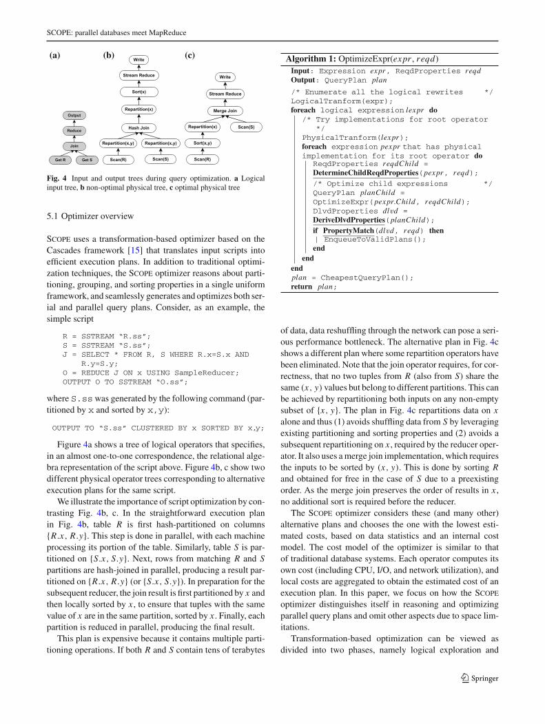
(a) (b) (c)

Fig. 4 Input and output trees during query optimization. a Logicalinput tree, b non-optimal physical tree, c optimal physical tree

5.1 Optimizer overview

Scope uses a transformation-based optimizer based on theCascades framework [15] that translates input scripts intoefficient execution plans. In addition to traditional optimi-zation techniques, the Scope optimizer reasons about parti-tioning, grouping, and sorting properties in a single uniformframework, and seamlessly generates and optimizes both ser-ial and parallel query plans. Consider, as an example, thesimple script

R = SSTREAM “R.ss”;S = SSTREAM “S.ss”;J = SELECT * FROM R, S WHERE R.x=S.x AND

R.y=S.y;O = REDUCE J ON x USING SampleReducer;OUTPUT O TO SSTREAM “O.ss”;

where S.sswas generated by the following command (par-titioned by x and sorted by x,y):

OUTPUT TO “S.ss” CLUSTERED BY x SORTED BY x,y;

Figure 4a shows a tree of logical operators that specifies,in an almost one-to-one correspondence, the relational alge-bra representation of the script above. Figure 4b, c show twodifferent physical operator trees corresponding to alternativeexecution plans for the same script.

We illustrate the importance of script optimization by con-trasting Fig. 4b, c. In the straightforward execution planin Fig. 4b, table R is first hash-partitioned on columns{R.x, R.y}. This step is done in parallel, with each machineprocessing its portion of the table. Similarly, table S is par-titioned on {S.x, S.y}. Next, rows from matching R and Spartitions are hash-joined in parallel, producing a result par-titioned on {R.x, R.y} (or {S.x, S.y}). In preparation for thesubsequent reducer, the join result is first partitioned by x andthen locally sorted by x , to ensure that tuples with the samevalue of x are in the same partition, sorted by x . Finally, eachpartition is reduced in parallel, producing the final result.

This plan is expensive because it contains multiple parti-tioning operations. If both R and S contain tens of terabytes

Algorithm 1: OptimizeExpr(expr , reqd)Input: Expression expr, ReqdProperties reqdOutput: QueryPlan plan

/* Enumerate all the logical rewrites */LogicalTranform(expr);foreach logical expression lexpr do

/* Try implementations for root operator*/

PhysicalTranform(lexpr);foreach expression pexpr that has physicalimplementation for its root operator do

ReqdProperties reqdChild =DetermineChildReqdProperties(pexpr, reqd);

/* Optimize child expressions */QueryPlan planChild =OptimizeExpr(pexpr.Child, reqdChild);DlvdProperties dlvd =DeriveDlvdProperties(planChild);

if PropertyMatch(dlvd, reqd) thenEnqueueToValidPlans();

endend

endplan = CheapestQueryPlan();return plan;

of data, data reshuffling through the network can pose a seri-ous performance bottleneck. The alternative plan in Fig. 4cshows a different plan where some repartition operators havebeen eliminated. Note that the join operator requires, for cor-rectness, that no two tuples from R (also from S) share thesame (x, y) values but belong to different partitions. This canbe achieved by repartitioning both inputs on any non-emptysubset of {x, y}. The plan in Fig. 4c repartitions data on xalone and thus (1) avoids shuffling data from S by leveragingexisting partitioning and sorting properties and (2) avoids asubsequent repartitioning on x , required by the reducer oper-ator. It also uses a merge join implementation, which requiresthe inputs to be sorted by (x, y). This is done by sorting Rand obtained for free in the case of S due to a preexistingorder. As the merge join preserves the order of results in x ,no additional sort is required before the reducer.

The Scope optimizer considers these (and many other)alternative plans and chooses the one with the lowest esti-mated costs, based on data statistics and an internal costmodel. The cost model of the optimizer is similar to thatof traditional database systems. Each operator computes itsown cost (including CPU, I/O, and network utilization), andlocal costs are aggregated to obtain the estimated cost of anexecution plan. In this paper, we focus on how the Scopeoptimizer distinguishes itself in reasoning and optimizingparallel query plans and omit other aspects due to space lim-itations.

Transformation-based optimization can be viewed asdivided into two phases, namely logical exploration and

123

J. Zhou et al.

physical optimization. Logical exploration applies transfor-mation rules that generate new logical expressions. Imple-mentation rules, in turn, convert logical operators to physicaloperators. Algorithm 1 shows a (simplified) recursive opti-mization routine that takes as input a query expression anda set of requirements. We highlight three different contextswhere reasoning about data properties occurs during queryoptimization.

– Determining child required properties. The parent (phys-ical) operator imposes requirements that the outputfrom the current physical operator must satisfy. For exam-ple, the output must be sorted on R.y. To functioncorrectly, the operator may itself impose certain require-ments on its inputs, for example, the two inputs to ajoin must be partitioned on R.x and S.x , respectively.Based on these two requirements, we must then determinewhat requirements to impose on the result of the inputexpressions. The function DetermineChildReqd-Properties is used for this purpose. If the require-ments are incompatible, a compensating operator (e.g.,sort or partition) would be added during the optimizationof the child operator by an enforcer rule (see Sect. 5.5.1).

– Deriving delivered properties. Once physical plans for thechild expressions have been determined, we compute thedata properties of the result of the current physical opera-tor by calling the functionDeriveDlvdProperties.A child expression may not deliver exactly the requestedproperties. For example, we may have requested a resultgrouped on R.x but the chosen plan delivers a result thatis, in addition, sorted on R.x . The delivered propertiesare a function of the delivered properties of the inputsand the behavior of the current operator, for example,whether it is hash or merge join. We explain this processin Sect. 5.4.1.

– Property matching. Once the delivered properties havebeen determined, we test whether they satisfy the requiredproperties, by calling the function PropertyMatch. Ifthey do not match, the plan with the current operator isdiscarded. The match does not have to be exact – a resultwith properties that exceed the requirements is accept-able. We cover the details in Sect. 5.4.3.

We next discuss some key operators in the Scope opti-mizer in Sect. 5.2, our property formalism in Sect. 5.3, rea-soning about data properties in Sect. 5.4, and domain-specifictransformation rules in Sect. 5.5.

5.2 Operators and parallel plans

The Scope optimizer handles all traditional logical and phys-ical operators from relational DBMSs, such as join and union

Fig. 5 Common subexpressions during optimization

variants, filters, and aggregates. It is also enhanced withspecialized operators that correspond to the user-definedoperators described in Sect. 4.4 (i.e., extractors, reducers,processors, combiners, and outputters). We next describetwo operators that allow the optimizer to reuse commonsubexpressions and to consider parallel plans in an integratedmanner.

5.2.1 Common subexpressions

As explained in Sect. 4, Scope allows programmers to writescripts as a series of simple data transformations. Due tocomplex business logics, it is common that scripts explicitlyshare common subexpressions. As an example, the follow-ing script fragment unions two sources into an intermediateresult, which is both aggregated and joined with a differentsource, producing multiple results that are later consumed inthe script:

...U = SELECT * FROM R UNION ALL SELECT * FROM S;G = SELECT a, SUM(b) FROM U GROUP BY a;J = SELECT * FROM U, T ON U.a = T.a AND

U.b = T.b;...

The optimizer represents common subexpressions byspool operators. Figure 5 shows the logical input to the opti-mizer for the fragment above. It is important to note thatspool operators generalize input and output trees to DAGs.A spool operators has a single producer (or child) and multi-ple consumers (or ancestors) in the operator DAG. Detailedcommon subexpression optimization with spool operatorscan be found in [33]. We also note that sharing expressedat the logical level does not necessarily translate into shar-ing in physical plans. The reason is subtle: it might be morebeneficial to execute the shared subexpression twice (eachone with different partitioning or sorting properties).

5.2.2 Data exchange

A key feature of distributed query processing is based on par-titioning data into smaller subsets and processing partitions

123


in parallel on multiple machines. This can done by a singleoperator, the data exchange operator, which repartitions datafrom n inputs to m outputs [14].

Exchange is implemented by one or two physical opera-tors: a partition operator and/or a merge operator. Each par-tition operator simply partitions its input while each mergeoperator collects and merges the partial results that belong toits result partition. Suppose, we want to repartition n inputpartitions, each one on a different machine, into m outputpartitions on a different set of machines. The processing isdone by n partition operators, one on each input machine, andm merge operators, one on each output machine. A partitionoperator reads its input and splits it onto m subpartitions.Each merge operator collects the data for its partition fromthe n corresponding subpartitions.

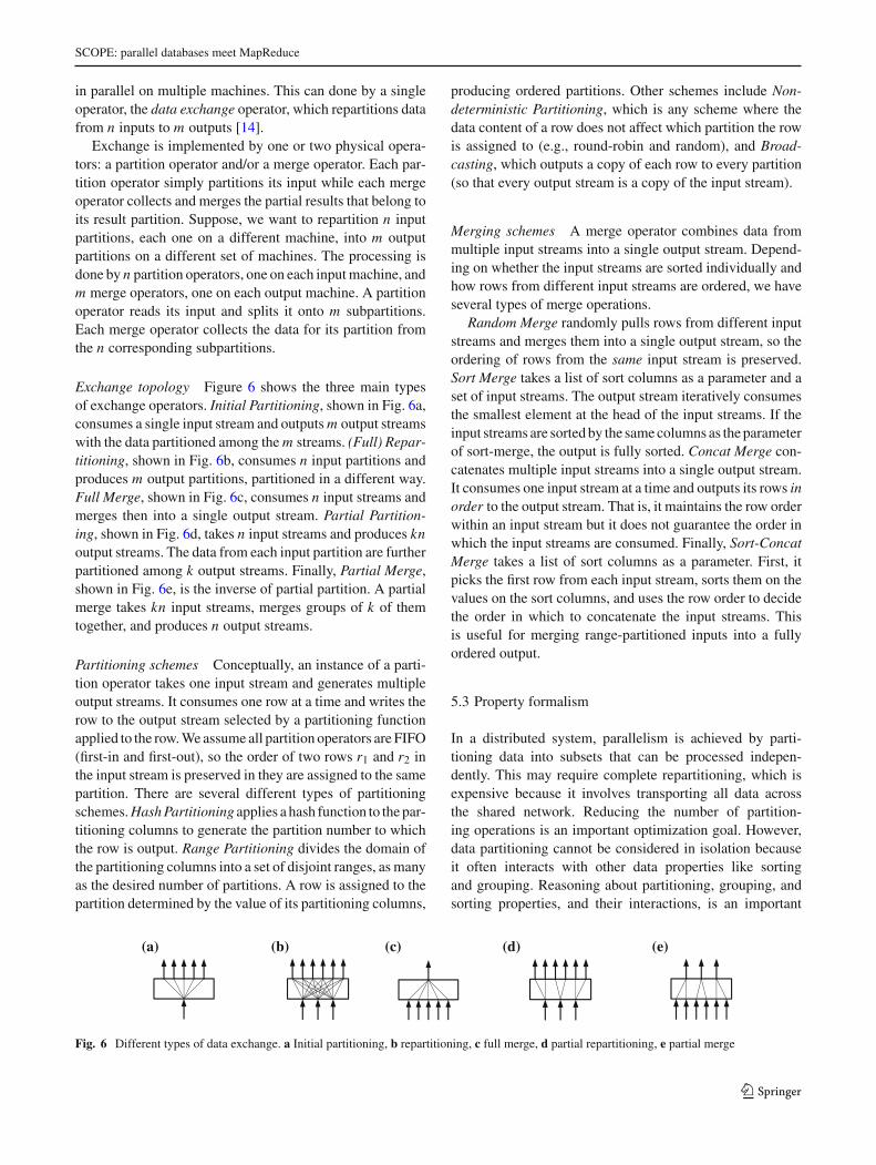
Exchange topology Figure 6 shows the three main typesof exchange operators. Initial Partitioning, shown in Fig. 6a,consumes a single input stream and outputs m output streamswith the data partitioned among the m streams. (Full) Repar-titioning, shown in Fig. 6b, consumes n input partitions andproduces m output partitions, partitioned in a different way.Full Merge, shown in Fig. 6c, consumes n input streams andmerges then into a single output stream. Partial Partition-ing, shown in Fig. 6d, takes n input streams and produces knoutput streams. The data from each input partition are furtherpartitioned among k output streams. Finally, Partial Merge,shown in Fig. 6e, is the inverse of partial partition. A partialmerge takes kn input streams, merges groups of k of themtogether, and produces n output streams.

Partitioning schemes Conceptually, an instance of a parti-tion operator takes one input stream and generates multipleoutput streams. It consumes one row at a time and writes therow to the output stream selected by a partitioning functionapplied to the row. We assume all partition operators are FIFO(first-in and first-out), so the order of two rows r1 and r2 inthe input stream is preserved in they are assigned to the samepartition. There are several different types of partitioningschemes. Hash Partitioning applies a hash function to the par-titioning columns to generate the partition number to whichthe row is output. Range Partitioning divides the domain ofthe partitioning columns into a set of disjoint ranges, as manyas the desired number of partitions. A row is assigned to thepartition determined by the value of its partitioning columns,

producing ordered partitions. Other schemes include Non-deterministic Partitioning, which is any scheme where thedata content of a row does not affect which partition the rowis assigned to (e.g., round-robin and random), and Broad-casting, which outputs a copy of each row to every partition(so that every output stream is a copy of the input stream).

Merging schemes A merge operator combines data frommultiple input streams into a single output stream. Depend-ing on whether the input streams are sorted individually andhow rows from different input streams are ordered, we haveseveral types of merge operations.

Random Merge randomly pulls rows from different inputstreams and merges them into a single output stream, so theordering of rows from the same input stream is preserved.Sort Merge takes a list of sort columns as a parameter and aset of input streams. The output stream iteratively consumesthe smallest element at the head of the input streams. If theinput streams are sorted by the same columns as the parameterof sort-merge, the output is fully sorted. Concat Merge con-catenates multiple input streams into a single output stream.It consumes one input stream at a time and outputs its rows inorder to the output stream. That is, it maintains the row orderwithin an input stream but it does not guarantee the order inwhich the input streams are consumed. Finally, Sort-ConcatMerge takes a list of sort columns as a parameter. First, itpicks the first row from each input stream, sorts them on thevalues on the sort columns, and uses the row order to decidethe order in which to concatenate the input streams. Thisis useful for merging range-partitioned inputs into a fullyordered output.

5.3 Property formalism

In a distributed system, parallelism is achieved by parti-tioning data into subsets that can be processed indepen-dently. This may require complete repartitioning, which isexpensive because it involves transporting all data acrossthe shared network. Reducing the number of partition-ing operations is an important optimization goal. However,data partitioning cannot be considered in isolation becauseit often interacts with other data properties like sortingand grouping. Reasoning about partitioning, grouping, andsorting properties, and their interactions, is an important

(a) (b) (c) (d) (e)

Fig. 6 Different types of data exchange. a Initial partitioning, b repartitioning, c full merge, d partial repartitioning, e partial merge

123

J. Zhou et al.

Table 1 Notation used in the paper

C1, C2, . . . Columns

X , Y, S, G, J Sets of columns

A, B Local structural properties

r1, r2, . . . Tuples

P1, P2, . . . Partitions

r [C], r [X ] Projection of r onto column C andcolumns X , respectively

∗ Any properties (including empty)

⊥, ∅, � Non-partitioned, randomly partitioned,and replicated global properties

foundation for query optimization in a distributed environ-ment.

A partition operation divides a relation into disjoint sub-sets, called partitions. A partition function defines whichrows belong to which partitions. Partitioning applies to thewhole relation; it is a global structural property. Groupingand sorting properties define how the data within each parti-tion is organized and are thus partition-local properties, hererefereed to as local structural properties. We next definethese three properties, collectively referred to as structural(data) properties. Table 1 summarizes the notation used inthis section.

5.3.1 Local structural properties

A sequence of rows r1, r2, . . . , rm is grouped on a set of col-umns X , denoted X g , if between two rows that agree in X ,there is no row with a different value in X . That is, if ∀ri , r j :i < j ∧ ri [X ] = r j [X ] ⇒ ∀k : i < k < j, rk[X ] = ri [X ].Similarly, a sequence of rows r1, r2, . . . , rm is sorted on acolumn C in an ascending (or descending) order, denotedby Co↑ (or Co↓ ), if ∀ri , r j , i < j ⇒ ri [C] ≤ r j [C] (orri [C] ≥ r j [C]). We use Co for simplicity when the contextis clear.

Definition 1 (Local structural properties) Local structuralproperties A are ordered sequences of grouping and sort-ing properties A = (A1, A2, . . . , An), where each Ai iseither X g or Co. A sequence of rows R = (r1, r2, . . . , rm)

satisfies local structural properties A if (1) R satisfies(A1, A2, . . . , An−1), and (2) every subsequence of R thatagrees on the values of columns in A1, A2, . . . , An−1 addi-tionally satisfies An .

We denote (A0 : A) to be the concatenation of a groupingor sorting property A0 to local structural properties A, thatis, (A0, A1, A2, . . . , An).

5.3.2 Global structural properties

There are two major classes of partitioning schemes, orderedand non-ordered. A non-ordered partitioning scheme ensuresonly that all rows with the same values of the partitioningcolumns are contained in the same partition. This is analo-gous to grouping as local property. More formally, a relationR is non-ordered partitioned on columns X with partition-ing function P if ∀r1, r2 ∈ R : r1[X ] = r2[X ] ⇒ P(r1) =P(r2).

An ordered partitioning scheme provides the additionalguarantee that the partitions cover disjoint ranges of the par-titioning columns. In other words, rows assigned to a partitionPi are either all less than or greater than rows in another par-tition P j . This is analogous to ordering as a local property.More formally, a relation R is ordered-partitioned into par-titions P1, P2, . . . , Pm on (Co1

1 , Co22 , . . . , Con

n ) where oi ∈{o↑, o↓}, if it satisfies the non-ordered partitioned conditionabove and, for each pair of partitions Pi and P j with i < j :

∀ri ∈ Pi , r j ∈ P j : ri [C1, . . . , Cn] <o1,...,on r j [C1, . . . , Cn]

where <o1,...,on is the multi-column comparison operator thattakes ascending/descending variants into account, so that forinstance (1, 2, 3) <o↑,o↓,o↑ (1, 5, 2).

Definition 2 (Global structural properties) Given a relationR and columns X = {C1, . . . Cn}, a global structural prop-erty can be (1)⊥, which indicates that data are not partitioned,(2) ∅, which indicates that data are randomly partitioned,(3) �, which indicates that data are completely duplicated,(4) X g , which indicates that R is non-ordered partitioned oncolumns X , and (5) (Co1

1 , . . . , Conn ), which indicates that R is

ordered partitioned on (Co11 , . . . , Con

n ). When it is clear fromthe context, we use (Co1

1 , . . . , Conn ), and X o interchangeably

for an ordered partitioned global property.

5.3.3 Structural properties

The structural properties of a relation R are specified by a pairof global structural property G and local structural proper-ties L, denoted as {G; L}. Additionally, a structural propertyalso defines the exact partitioning function and the numberof partitions, which we omit in this work for the clarity ofexposition.

Table 2 shows an instance of a relation with three columns{C1, C2, C3}, and structural data properties {{C1}g; ({C1,

C2}g, Co3 )}. In words, the relation is partitioned on col-

umn C1 and, within each partition, data are first grouped oncolumns C1, C2, and, within each such group, sorted by col-umn C3.

123


Table 2 Relation with partitioning, grouping, and sorting

Partition 1 Partition 2 Partition 3

{1,4,2}, {1,4,5}, {7,1,2} {4,1,5}, {3,7,8}, {3,7,9} {6,2,1}, {6,2,9}

5.4 Structural properties and query optimization

We next describe how the optimizer reasons about data prop-erties in the three contexts outlined in Algorithm 1.

5.4.1 Deriving structural properties

We first consider how to derive the structural properties ofthe output of a physical operator. Earlier research has shownhow to derive ordering and grouping properties for standardrelational operators executed on non-partitioned inputs [21,22,25,26,30]. Ordering and grouping are local properties,that is, properties of each partition, so previous work stillapplies when the operators are running in partitioned mode.What remains is to reason with global partitioning proper-ties throughout a query plan and their interaction with localproperties.

Properties after a scan operator Recall from Sect. 3 thatdata can be stored either as unstructured or structuredstreams. The scan operator over an unstructured stream deliv-ers a random partitioning. More interestingly, reading a struc-tured stream delivers the partitioning and sorting propertiesthat are defined in the structured stream itself. This can beuseful to avoid further repartitioning operations whenever therequired properties of a subsequent operator can be satisfiedby the delivered properties of the structured stream itself.

Properties after a partitioning operator Partition operatorsare assumed to be FIFO, that is, they output rows in the sameorder that they are read from the input. Thus, they affectthe global properties but not local properties. Every outputpartition inherits the local properties (sorting and grouping)of its input. Table 3 summarizes the properties of the out-put after an initial partitioning operator when the input hasstructural properties {X θ ;A}. Hash partitioning on columnsC1, C2, . . . , Cn produces a non-ordered collection of parti-tions, which is indicated in the table with the global structuralproperty {C1, C2, . . . , Cn}g . Range partitioning on columnsC1, C2, . . . , Cn produces an ordered collection of partitions,which is indicated in the table with global structural prop-erty (Co1

1 , Co22 , . . . , Con

n ). In a non-deterministic partition-ing scheme (round-robin and random partitioning), a row ispartitioned independent on its content, so we indicate thisby ∅.

Table 3 Structural properties of the result after partitioning an inputwith properties {X ; A}Scheme Result

Hash on C1, . . . , Cn {{C1, . . . , Cn}g; A}Range on Co1

1 , . . . , Conn {(Co1

1 , . . . , Conn ); A}

Non-deterministic {∅; A}Broadcast {�; A}

Properties after a merge operator A full merge operatorproduces a single output. Its local properties depend on thelocal properties of the input and the merge operator type:random merge, sort-merge, concat merge, and sort-concatmerge.

Table 4 summarizes the structural properties after a fullmerge, depending on the type of merge operator and whetherthe input partitioning is ordered or non-ordered. A randommerge does not guarantee any row order in the result, so nolocal properties can be derived for the output. For a sort-merge, there are two cases. If the local properties of theinput imply that the input streams are sorted on the col-umns used in the merge (see Sect. 5.4.3 for more details onproperty inference), the output will be sorted, otherwise not.A concat merge operator maintains the row order within eachsource partition. If each source partition is grouped in a sim-ilar way to how it is non-ordered partitioned, the result ofis also grouped, otherwise not. Finally, a sort-concat mergeproduces a sorted result if inputs are range partitioned andeach partition is also sorted on the same columns as it ispartitioned on.

Example 1 A sort-concat full merge on {Co1 , Co

2 } of inputswith properties {(Co

1 , Co2 ); (Co

1 , Co2 , Cg

3 )} generates an out-put with properties {⊥; (Co

1 , Co2 , Cg

3 )}.

Properties after a repartitioning operator The propertiesof the result after repartitioning depend on the partitioningscheme, the merge scheme, and the local properties of theinput. Table 5 summarizes the structural properties after rep-artitioning an input with properties {∗;A}.Example 2 Given inputs with properties {{C1, C2}g;(Co

2 , Co1 , Co

3 )}, concat merging generates an output withproperties {{C1, C2}g; ({C1, C2}g, Co

3 )}, for repartitioning,and {⊥; ({C1, C2}g, Co

3 )}, for a full merge.

5.4.2 Deriving required structural properties

We now consider how to determine required properties of theinputs for different physical operators. Table 6 lists requiredinput properties for the most common physical operators.

123

J. Zhou et al.

Table 4 Structural propertiesof the result after a full merge Input properties {X g; A} Input properties {X o; A}

Random merge {⊥; ∅} {⊥; ∅}Sort merge on So (1). {⊥; So} if A ⇒ So (1). {⊥; So} if A ⇒ So

(2). {⊥; ∅} otherwise (2). {⊥; ∅} otherwise

Concat merge (1). {⊥; (X g : B)} if A ⇒ (X g : B) (1). {⊥; (X g : B)} if A ⇒ (X g : B)


Sort-concat merge on So (1). {⊥; (X g : B)} if A ⇒ (X g : B) (1). {⊥; A} if So ⇔ X o and A ⇒ So


Table 5 Structural properties of the result after repartitioning on X with input properties {∗; A}Hash partitioning Range partitioning Non-determ. partitioning

Random merge {X g; ∅} {X o; ∅} {∅; ∅}Sort merge on So {X g; So} if A ⇒ So {X o; So} if A ⇒ So {∅; So} if A ⇒ So

{X g; ∅} otherwise {X o; ∅} otherwise {∅; ∅} otherwise

Concat merge {X g; (X g : B)} if A ⇒ (X g : B) {X o; (X g : B)} if A ⇒ (X g : B) {∅; (X g : B)} if A ⇒ (X g : B)


Sort-concat merge on So {X g; (X g : B)} if A ⇒ (X g : B) {X o; A} if So ⇔ X o and A ⇒ So {∅; A} if So ⇔ X o and A ⇒ So


Table 6 Required structural properties of inputs to common physical operators

Non-partitioned version Partitioned version

Table scan, select, project {⊥; ∗} {X θ ; ∗}, X �= ∅Hash aggregate on G {⊥; ∗} {X θ ; ∗},∅ ⊂ X ⊆ GStream aggregate on G {⊥; (Gg)} {X θ ; (Gg)},∅ ⊂ X ⊆ GNested-loop or hash join

(equijoin on columnsJ1 ≡ J2)

Both inputs {⊥; ∗} Pair-wise Join:Input 1: {X θ ; ∗},∅ ⊂ X ⊆ J1; Input 2: {Yθ ; ∗},∅ ⊂ Y ⊆ J2; X ≡ YBroadcast Join:Input 1: {�; ∗}; Input 2: {X θ ; ∗}, X �= ∅

Merge join (equijoin oncolumns J1 ≡ J2)

Input 1: {⊥; J o1 } Pair-wise Join:

Input 2: {⊥; J o2 } Input 1: {X θ ; J o

1 },∅ ⊂ X ⊆ J1; Input 2: {Yθ ; J o2 },∅ ⊂ Y ⊆ J2; X ≡ Y

Broadcast Join:Input 1: {�; J o

1 }; Input 2: {Y; J o2 }, Y �= ∅

Note that for the purpose of property derivation, we treatcombiners and reducers as joins and aggregates, respectively.Depending on whether the operator is executed in eitherpartitioned or non-partitioned mode, it imposes differentrequirements on its inputs. A non-partitioned operator runs asa single instance and produces non-partitioned data. A parti-tioned operator runs as multiple instances, each instance con-suming and producing only partitions of the data. However,not all operators can be executed in parallel. For instance,aggregation with no group-by columns can only be executedin non-partitioned mode.

Table scan, select and project process individual rows andimpose no requirements on their inputs (i.e., it does not mat-

ter how the input data are partitioned, sorted, or grouped).Thus, their input requirements are shown as {X θ ; ∗} whereX can be any set of columns.

For a hash aggregation to work correctly, all rows withthe same value of the grouping columns must be in a singlepartition. This is guaranteed as long as the input is partitionedon a subset of the grouping columns. A stream aggregationalso requires that the rows within each partition be groupedon the grouping columns.

We consider two types of partitioned joins: pair-wise joinand broadcast join. A pair-wise join takes two partitionedinputs. The inputs must be partitioned on a subset of the joincolumns in the same way (i.e., on the same set of equivalent

123


columns and into the same number of partitions). Broadcastjoin takes one partitioned input (it does not really matter howit is partitioned) and a second input that is replicated (broad-cast) to each partition of the first input. A merge join has theadditional requirement that each partition be sorted on thejoin columns.

Example 3 Suppose, we are considering using a partitionedmerge join to join tables R and S on R.C1 = S.C1 andR.C2 = S.C2. Based on the rules in Table 6, both inputsmust be partitioned and sorted in the same way. The partition-ing columns must be a subset of or equal to the join columns({R.C1, R.C2} and {S.C1, S.C2}, respectively). The sort col-umns must also be equal to the join columns on each input.Each of the following requirements satisfies the restrictionsand is thus valid input requirements. We do not list all pos-sibilities here and also leave the exact sort order, o↑ and o↓,unspecified.

– {R.Cg1 ; (R.Co

2 , R.Co1 )} and {S.Cg

1 ; (S.Co2 , S.Co

1 )}– {R.Co

2 ; (R.Co1 , R.Co

2 )} and {S.Co2 ; (S.Co

1 , S.Co2 )}

– {{R.C1, R.C2}g; (R.Co2 , R.Co

1 )} and{{S.C1, S.C2}g; (S.Co

2 , S.Co1 )}

As shown by the example, the requirements in Table 6for the child expressions are not always unique and canbe satisfied in several ways. For instance, aggregation on{C1, C2} requires the input to be partitioned on {C1}, {C2}, or{C1, C2}. Conceptually, each requirement corresponds to onespecific implementation. This situation could be handled bygenerating multiple alternatives, one for each requirement.However, this approach would generate a large number ofalternatives, making optimization more expensive. Instead,we allow required properties to cover a range of possibili-ties and rely on enforcer rules, described in Sect. 5.5.1, togenerate valid rewrites. To this end, the optimizer encodesrequired structural properties as follows.

– Partitioning requirement, which can be either broad-cast (�), non-partitioned (⊥), or a partition requirementincluding minimum partitioning columns Xmin and max-imum partitioning columns Xmax

(∅ ⊆ Xmin ⊆ Xmax).– Sorting requirement, which consists of a sequence of sort-

ing columns (So1 , So

2 , . . . , Son ), o ∈ {o↑, o↓}.

– Grouping requirement, which consist of a set of groupingcolumns {G1, G2, . . . , Gn}g .

In the previous example of aggregation on {C1, C2}, the par-titioning requirement is any subset of the grouping columns,so Xmin = ∅,Xmax = {C1, C2}. This requirement is satis-fied by a hash or range partition with column set X whereXmin ⊂ X ⊆ Xmax.

Some operators are by themselves invariant to partition-ing and ordering (e.g., filters) and simply pass parent require-ments down to their children.

User-defined operators deserve a special mention. In prin-ciple, a Processor can execute arbitrary code to produceoutput rows given its input. Therefore, it would seem thatany property inference cannot propagate past such opera-tors. The properties described in Sect. 4.4.1 provide a wayfor users to specify additional information to the optimizer.For instance, if a processor marks a column as pass-through,it essentially means that input and output rows would satisfyall structural properties on such column. Therefore, we canpush down a partitioning requirement through a processor asfor the case of filters whenever all the structural property col-umns are marked as pass-through. These and other properties(e.g., column dependencies) are also used to determine therequired output columns from a child operator, essentiallyperforming a guided data-flow analysis on the query DAG.

The rules in Table 6 do not consider requirements imposedon the operator by its parent. In that case, some operatorsare able to do early pruning due to conflicting properties.For instance, if a merge join is required to produce a resultsorted on (C1, C2) but its equality join predicates are onC3, there is no merge join implementation that could sat-isfy its sorting requirements, assuming that sorting on (C3)

does not imply sorting on (C1, C2). This merge join is aninvalid alternative—it can never produce an output that sat-isfies the requirements. The optimizer checks for such invalidalternatives and discards them immediately.

5.4.3 Property matching

The optimizer ensures that a physical plan is valid bychecking that its delivered properties satisfy the requiredproperties. Property matching checks whether one set ofproperties {X θ1;A} satisfies another {Yθ2;B}, that is, whether{X θ1;A} ⇒ {Yθ2;B}. Matching of structural properties isdone by matching global and local properties separately:

({X θ1;A} ⇒ {Yθ2;B}) ⇔ (X θ1 ⇒ Yθ2 ∧ A ⇒ B)

Two structural properties may be equivalent even if theyappear different because of column equivalences (e.g., viajoins) or functional dependencies. Normalization and match-ing of local properties (sorting and grouping) have beenstudied extensively in [21,22]. We next review functionaldependencies, constraints, and column equivalences, andthen describe a number of inference rules to reason withstructural properties.

A set of columns X functionally determines a set of col-umns Y , if for any two rows that agree on the values of

123

J. Zhou et al.

columns in X , they also agree on values of columns in Y .We denote such functional dependency by X → Y .

Functional dependencies appear in several ways:

Trivial FDs: X → Y whenever X ⊇ Y .Key constraints: Keys are a special case of functionaldependencies. If X is a key of relation R, then X func-tionally determines every column of R.Column equality constraints: A selection or join with apredicate C1 = C2 implies that the functional dependen-cies {C1} → {C2} and {C2} → {C1} hold in the result.Constant constraints: After a selection with a predicateC = constant all rows in the result have the same valuefor column C . This can be viewed as a functional depen-dency which we denote by ∅ → C .Grouping columns: After a group-by with columns X , Xis a key of the result and, thus, functionally determines allother columns in the result.

If all tuples of a relation must agree on the values of aset of columns, such columns belong to a column equiva-lence class. An equivalence class may also contain a con-stant, which implies that all columns in the class have thesame constant value. Equivalence classes are generated byequality predicates, typically equijoin conditions and equal-ity comparisons with a constant.

Both functional dependencies and column equivalenceclasses can be computed bottom up in an expression tree [10,21,22,26], and in the following, we assume that these havebeen computed.

Inference rules

We next briefly discuss inference rules for structural prop-erties. The first rule shows that local properties can betruncated.

{∗; (A1, . . . , Am−1, Am)} ⇒ {∗; (A1, . . . , Am−1)} (1)

Global properties cannot be truncated but they can beexpanded. A result that is partitioned on columns C1, C2 isnot partitioned on C1 because two rows with the same valuefor C1 may be in different partitions. However, a result par-titioned on C1 alone is in fact partitioned on C1, C2 becausetwo rows that agree on C1, C2 also agree on C1 alone and,consequently, they are in the same partition. More formally,

{{C1, . . . , Cm}g; ∗} ⇒ {{C1, . . . , Cm, Cm+1}g; ∗} (2)

{(Co11 , . . . , Com

m ); ∗} ⇒ {(Co11 , . . . , Com

m , Com+1m+1 ); ∗} (3)

If a sequence of rows is sorted, it is also grouped, so:

{∗; (A1, . . . , Co, . . . , Am)}⇒{∗; (A1, . . . , {C}g, . . . , Am)}(4)

{(Co11 , . . . , Con

n ); ∗} ⇒ {{C1, . . . , Cn}g; ∗} (5)

Functional dependencies allow us to eliminate groupingcolumns from both global and individual local structuralproperties:

if ∃ C ∈ X : (X − {C}) → C, then X g ⇒ (X − {C})g

(6)

The following rule can be applied to eliminate sortingcolumns in global structural properties:

if ∃ {C1, . . . , Ci−1} → Ci , then

{{Co11 , . . . , Coi−1

i−1 , Coii , Coi+1

i+1 , . . .};A}⇒ {{Co1

1 , . . . , Coi−1i−1 , Coi+1

i+1 , . . .};A} (7)

Finally, the following rule eliminates individual localstructural properties altogether:

if X1 ∪ . . . ∪ Xi−1 → Xi , then

{∗; (X θ11 , . . . ,X θi−1

i−1 ,X θii ,X θi+1

i+1 , . . .)}⇒ {∗; (X θ1

1 , . . . ,X θi−1i−1 ,X θi+1

i+1 , . . .)}. (8)

Property normalization

To simplify property matching, properties are converted to anormalized form. The basic idea of the normalization proce-dure is as follows. First, in each partitioning, sorting, group-ing property, and functional dependency replace each columnwith the representative column in its equivalence class. Then,in each partitioning, sorting and grouping property removecolumns that are functionally determined by some other col-umns. We illustrate this procedure with an example.

Example 4 We want to test whether the structural propertiesP1 = {{C7, C1, C3}g; (C

o↑6 , C

o↓2 , C

o↑5 )} satisfy the structural

properties P2 = {{C1, C2, C4}g; ({C1, C2}g)}. We know thatthe data satisfy the functional dependency {C6, C2} → {C3}.There are two column equivalence classes {C1, C6} and{C2, C7} with C1 and C2 as representative columns, respec-tively. After replacing columns by representative columns,we have that:

P1 = {{C2, C1, C3}g; (Co↑1 , C

o↓2 , C

o↑5 )}

P2 = {{C1, C2, C4}g; ({C1, C2}g)}{C1, C2} → {C3}.

123


Next, we apply the functional dependency to eliminate C3,which changes P1 to {{C2, C1}g; (C

o↑1 , C

o↓2 , C

o↑5 )} while P2

is unchanged.We first consider global properties. We want to prove that

{C2, C1}g ⇒ {C1, C2, C4}g . According to the expansionrule for global properties (inference rule (2)), the implica-tion holds and thus the global properties match. Next, forlocal properties, we need to show that (C

o↑1 , C

o↓2 , C

o↑5 ) ⇒

({C1, C2}g). Applying the truncation rule for local properties(inference rule (1)), we obtain (C

o↑1 , C

o↓2 ) ⇒ ({C1, C2}g)

because sorting implies grouping (inference rule (4)). Sinceboth global and local properties match, P1 satisfy P2.

5.5 The rule set

A crucial component in our optimizer is the rule set. In fact,the set of rules available to the optimizer is one of the deter-mining factors in the quality of the resulting plans. Many ofthe traditional optimization rules from database systems areclearly applicable also in our context, for example, remov-ing unnecessary columns, pushing down selection predicates,and pre-aggregating when possible. However, the highly dis-tributed execution environment offers new opportunities andchallenges, making it necessary to explicitly consider theeffects of large-scale parallelism during optimization. Forexample, choosing the right partition scheme and decidingwhen to partition are crucial for finding an optimal plan. It isalso important to correctly reason about partitioning, group-ing, and sorting properties, and their interaction, to avoidunnecessary computations.

5.5.1 Enforcer rules

Query optimizers in database systems typically start with anoptimal serial plan and then add parallelism in a postpro-cessing step. This approach may result in sub-optimal plans.The challenge is to seamlessly integrate consideration ofparallel plans into the normal optimization process. In thissection, we describe optimization rules that automaticallyintroduce data exchange operators and thus seamlessly gen-erate and optimize distributed query plans. We enhance theoptimization framework in two ways. First, for each log-ical operator, we consider both non-partitioned and parti-tioned implementations, as long as they can ever satisfytheir requirements. Second, we rely on a series of enforcerrules (explained below) to modify requirements for structuralproperties, say, from non-partitioned to partitioned, or fromsorted to non-sorted, etc. Together, with other optimizationrules and property inferences, this enables the optimizer toconsider both serial and parallel in a single integrated frame-work. It greatly enhances the power of a traditional queryoptimizer without dramatic infrastructure changes.

We begin with a simple example of sort optimization. Sup-pose that, during optimization, there is a request to optimizean expression with a specific local sort requirement S2. Theoptimizer then considers different alternative physical oper-ators for the root operator of the expression tree, derives whatproperties their inputs must satisfy, and requests an optimalplan for each input. There are typically three possible ways ofensuring that the result will be sorted. It is up to the optimizerto choose the best plan based on its cost estimates.

– If a physical operator itself can generate a sorted output,try this operator and push requirements imposed by theoperator itself to its child expressions.

– If a physical operator retains the input order, try the oper-ator and push the sort requirement plus requirements ofthe operator itself to its children.

– Otherwise, try the operator but add an explicit sort match-ing the requirement and then optimize the child expres-sions without the sort requirement.

In the last case, the optimizer enforces a sort requirementon top of the physical operator. We call such optimizationrules enforcer rules. Grouping requirements can be handledin a similar way, except we may not have an explicit group-only operator. A grouped result is usually produced as aside effect of another operator, for example, a one-to-manynested-loop join.

A data exchange operator is similar to sorting. Its onlyeffect is to change structural properties; it does not add oreliminate rows, nor does it modify individual rows in anyway. Therefore, we model data exchange operators as enforc-ers of structural properties.

Algorithm 2 shows simplified pseudo-code for enforcingpartitioning. For simplicity, handling of sorting and group-ing requirements is not shown. When a sorting requirementexists, we consider both sort-merge exchange and regularexchange operations. We also ignore the details of the parti-tioning requirement.

Although the pseudo-code is much simplified, it capturesthe core ideas of enforcing partitioning requirements. Forany expression with particular partitioning requirements, theoptimizer (1) uses an operator that itself satisfies the require-ments, (2) uses a partition-preserving operator and pushes therequirements to its children, (3) adds data exchange opera-tors that allow the requirements for its child expressions to berelaxed or modified. The optimizer tries all the alternativesand selects the best plan based on estimated costs.

2 For global sort requirements, such as those coming from ORDER BYclauses, the optimizer considers an alternative that requires its input tobe both range partitioned and locally sorted by the original sort columns,which is subsequently handled by the enforcer rules.

123

J. Zhou et al.

Algorithm 2: EnforceDataExchange(expr , reqd)Input: Expression expr, ReqdProperties reqd

ReqdProperties reqd New;Plan plan;if Serial(reqd) then

/* Require a serial output */reqd New = GenParallel(reqd);plan =AddExchangeFullMerge(OptimizeExpr(expr,reqd New));

else/* Require a parallel output. Enumerate

all possible partitioning alternativessuch that Xmin ⊆ X ⊆ Xmax */

cPlans = {};foreach valid partition schema X do

/* Case 1: repartition. Generate newpartitioning requirements for itschildren; remove specificpartitioning columns */

reqd New = GenParallel(reqd);cPlans +=AddExchangeRepartition(OptimizeExpr(expr,reqd New));/* Case 2: initial partition. Force

the child to generate a serialoutput */

cPlans += AddExchangeInitialPartition(Opti-mizeExpr(expr, reqd New));

plan = GetCheapestPlan(cPlans);end

endreturn plan;

Enforcer rules can seamlessly enable a single instance ofan operator to work on a partitioned input by introducing afull merge operator, multiple instances of an operator to workon a non-partitioned input by introducing an initial partitionoperator, and also multiple instances of an operator with spe-cific partitioning requirements to work on any partitionedinput sets by introducing a repartition operator. The numberof alternatives generated by enforcers could be large so usu-ally the optimizer applies cost-based heuristics to prioritizealternatives and prune out less promising ones.

5.5.2 Other specialized rules

In addition to the rules described earlier, the optimizer hasseveral exploration rules that deal with user-defined opera-tors (e.g., processors and reducers). We next briefly describesome of these specialized rules.

– Pushing selections below processors and reducers. Byleveraging pass-through columns (Sect. 4.4.1), we pushselection predicates below processors and reducers pro-vided that all predicate columns are annotated as pass-

through. This is required even if the input and outputschemas of a processor have the same names, as in gen-eral the values of such columns in input and output rowsmight not be correlated.

– Unfolding recursive reducers into local/global pairs.A recursive reducer requires that the input and outputschemas be identical. In these situations, we can explorean alternative that performs partial reduction on inputsthat are not necessarily partitioned by the reducer col-umns. These partial results are usually smaller than theraw input, and we can obtain the final result by reparti-tioning them and performing a final global reducer. Thisis similar to the traditional local/global aggregate optimi-zation in relational databases.

– Pushing processors and reducers below unions: Similarto the optimization that pushes filters closer to the sourcetables, the Scope optimizer considers alternatives thatpush down processors below union-all operators. If theoperator is a reducer, this optimization cannot always bedone, since for correctness the children of the union-allmust each have a distinct set of values for the reduc-ing columns. In that case, however, we can leveragethe previous optimization and convert a reducer into alocal/global pair. The local reducer can be pushed belowthe union all, effectively pre-aggregating data and result-ing in a more efficient plan. Also, if the optimizer candeduce that the values of the reducing columns on eachchildren of a union-all operator are disjoint (leveragingconstraints or script annotations), the optimizer can effec-tively push the reducer below the union all without requir-ing a global reducer afterwards, greatly improving overallperformance of the resulting execution plans.

6 Code generation and runtime engine

The Scope runtime engine implements a rich class ofcomposable physical operators. It supports variousimplementation of relational operations, such as filtering,projection, sorting, aggregation, and join. For instance,Scope provides three join operators: sort-merge join, (index)nested-loop join, and hash join. The engine contains a fewbuilt-in and optimized UDOs for common tasks. For exam-ple, DefaultTextExtractor and DefaultTextOutputter are pro-vided for users to extract inputs from and output results totext files. The engine supports different access methods forstructured streams, including table scan and index lookup.

Each Scope operator implements open, next, and closefunctions that allow a parent operator to get the result onetuple at a time. Such database-like iterator interface supportspipelining of operators naturally.

After optimization, a physical execution tree is generated.The runtime engine performs the following tasks. First, the

123


engine walks through the plan bottom up and generates codefor the corresponding operator, based on internal operatortemplate. Then, it combines a series of physical operatorsinto a super vertex, obtained by splitting the output tree atexchange and spool operators. In addition to these mandatorysuper vertex boundaries, it sometimes breaks large super ver-tices into smaller ones to avoid having execution units that runfor a long time (and thus would make recovery in the pres-ence of failures more time-consuming). All the generatedcode is compiled into an assembly, and the entry functionfor each super vertex is written into a super vertex defini-tion file. Each super vertex is scheduled and executed in onemachine. Operators within a super vertex are executed in away very similar to a single-node database engine. Specifi-cally, every super vertex is given enough memory to satisfyits requirements (e.g., hash tables or work tables for sorts),up to a certain fraction of total available memory and a frac-tion of the available processors. This procedure sometimesprevents a new super vertex from being run immediately on abusy machine. Similar to traditional database systems, eachmachine uses admission control techniques and queues out-standing super vertices until the required resources are avail-able. As we discuss later, in contrast to DBMSs, the overallsystem has additional scheduling choices for such queuedsuper vertices that reduce overall latency.

The output of the compilation of a script thus consistsof three components: (1) the algebra file that enumerates allsuper vertices and the data flow relationships among them,(2) the super vertex definition file, which contains the spec-ification and entry points in the generated code for all supervertices, and (3) the assembly itself, which contains the gen-erated code. This package is sent to the cluster for execution.

The Scope code generation mechanism is flexible andcan generate specific and highly optimized code for a script.The system knows precisely the input and output schema foreach operator. The generated code is specific to the schemasand completely avoids any runtime tuple interpretation. Thesystem also has many opportunities to further optimize thegenerated code. For instance, the intermediate record formatcan be changed to address the needs of subsequent operators.

6.1 Execution model

During execution, a super vertex reads inputs either locallyor remotely. Operators within a super vertex are executed in apipelined fashion. The final result of a super vertex is writtento local disks, waiting for the next vertex to pull data. Thispull execution model is much like to the MapReduce exe-cution model. However, the Scope engine does not requireevery function to be mapped into a super vertex as in theMapReduce model, potentially in a unnatural way. The opti-mizer has great flexibility to break arbitrary functions intosuper vertices based on a principled cost model.

This execution model is very different from that of tra-ditional parallel databases, which is optimized to avoid hit-ting disks and instead transfer intermediate data on the fly.Passing data on the fly requires that both producer and con-sumer machines are running concurrently and extensive syn-chronization between them. This approach does not scale tothousands of machines and is less reliable when one of theinvolved machines can crash in the middle of execution.

The pull execution model and materializing intermediateresults to disk may sound inefficient at first glance. However,it has many advantages in the context of highly distributedcomputation. First, it does not require both producer and con-sumer vertices to run concurrently, which greatly simplifiesjob scheduling. As we shall describe in Sect. 7, the job man-ager guarantees the two vertices are executed in sequence andhas great flexibility when to schedule the vertices. Second, allintermediate results are written to local disks. In case of ver-tex failures, which are inevitable, all that is required is rerunthe failed vertex from the cached inputs on disks. Only a smallportion of a query plan may need to be re-executed. Finally,writing intermediate results to disks frees system memory toexecute other vertices and simplifies computation resourcemanagement.

6.2 Runtime data exchange

We next describe in some detail the support of data exchangeoperations in the Scope runtime engine. Having efficientimplementations of such operators is crucial as data shufflingis a common and expensive operation. The Scope runtimeengine supports multiple variants of partitioning and merg-ing operators. For merging operators, the system attempts tooverlap network transfer with subsequent operations as muchas possible.

For partitioning operators, Scope supports hash and rangepartitioning over one or more columns. The total number ofpartitions can be either predefined or determined at runtimebased on intermediate data size.

Hash partitioning: A hash value is computed from the parti-tioning columns and taken modulo the number of total par-titions to get the destination partition.

Range partitioning: Calculating partitioning boundaries thatproduce partitions of uniform size is crucial for avoiding out-liers and achieving high query performance but challengingin a distributed fashion. Figure 7 presents a job graph thatthe Scope uses to range partition the input into 250 buck-ets. First, each input machine generates a local histogramover its local data. Second, a single coordinator combinesall the local histograms and calculate the partition bound-aries based on the global histogram (a detailed descriptionof histogram computation is beyond the scope of this paper).Finally, partitioning information is broadcast to all the input

123

J. Zhou et al.

Fig. 7 Range partitioning

machines, which then partition their local data accordingly.This dynamic partitioning strategy greatly improves parti-tioning quality.

Index-based partitioning: Independent of partitioning type,the partitioned outputs are first written to local disks in sep-arate files. When the number of partitions is large, writ-ing too many intermediate files at the same time incurslots of random I/O and significantly increases the overalllatency. The Scope runtime engine supports a novel par-titioning operation that relies on the indexing provided bystructured streams. For each tuple, the destination partitionID, called “PID,” is calculated using the partition func-tion in a normal way and is added to the tuple as a vir-tual column. A stable sort on PID is performed, so thatthe original tuple order within the same PID value is main-tained. (This is crucial when maintaining the tuple orderwithin each partition is required for subsequent operators).The sorted results are finally bulk written into a singleindex file. The following merging operator reads the cor-responding partition by index lookup on the desired PID.Index-based partitioning allows the system to partition largedata into thousands of partitions without penalizing the I/Osystem.

7 Job scheduling

Execution of a Scope job is coordinated by a job manager(JM), adapted from Dryad [17]. The JM is responsible forconstructing the job graph and scheduling work across theavailable resources in the cluster. As described in Sect. 6, aScope execution plan consists of a DAG of Scope super verti-ces that can be scheduled and executed on different machinesindependent of each other. The JM groups distinct types ofvertices into separate stages to simplify job management.All the vertices in a stage perform the same computation,defined in the query plan, on a different partition of inputdata. The JM maintains the job graph and keeps track of thestate and history of each vertex in the graph.

Fig. 8 Scope job scheduling

7.1 Job manager overview

Figure 8 shows a simplified overview of scheduling a Scopejob. Each machine in the cluster is capable of both data stor-age and computation. Besides storage services (not shownin the figure), a processing node (PN) service runs on eachmachine to manage local system resources (e.g., memory anddisk) and schedules execution of local vertices. PN nodesmaintain a local queue of vertex execution requests from dif-ferent JMs and create processes on behalf of the JMs takinginto account vertex priorities and available resources. Thefirst time a vertex is executed on a machine, its assembly issent from the JM to the PN and subsequently it is executedfrom a cache. PN also monitors the state of each running ver-tex, such as whether it succeeds or fails and how much datahave been read and written, and communicates the informa-tion back to the JM periodically through a heartbeat mech-anism. This feedback mechanism allows the JM to monitorthe time a super vertex is queued a busy PN machine; Ifnecessary, the JM can schedule duplicate instances of long-delayed vertices on different machines to reduce latencies.Whenever the first instance of a super vertex starts executing,all duplicate instances are eliminated from the correspondingPN queues.

When the job starts, the system picks one machine tolaunch the JM, which becomes responsible for schedulingthe Scope job. An initial DAG is built to track relation-ship among different vertices. As we shall describe later inSect. 7.2, the job graph may adapt itself dynamically as theexecution proceeds and system environment changes. Whenall of a vertex’s inputs become ready, the JM considers thevertex runnable and places it in a scheduling queue. Theactual vertex scheduling order is based on vertex priorityand resource availability. One scheduling principle is basedon data locality. That is, the JM tries to schedule the vertex

123


on a machine that stores or is close to its input wheneverpossible. If the selected machine is temporarily overloaded,the JM may scale back to another machine that is close innetwork topology (possibly in the same rack), so reading theinput can be done efficiently with minimum network traffic.A Scope vertex may also specify a “constraint” listing a pre-ferred set of machines to run. Once the machine is chosen,the JM places a request to run the vertex, together with itsassemblies, onto its PN queue.

For each vertex, the JM keeps track of all of inputs’ avail-ability and locations. It has no information about the actualcomputation performed by the vertex but it receives initialestimates of resource consumption from the optimizer. Asthe job proceeds, the JM tracks actual resource consump-tion for vertices in a stage. This information is used to refineresource estimates for the remaining vertices in the samestage to improve the local scheduling decisions made byPNs.

When a vertex execution fails for any reason, the JM isinformed. The failure could be due to user code errors orsystem transient failures, such as machine reboot or networktemporal congestion. Depending on the failure type, the JMapplies different policies and acts accordingly, including fail-ing the job or retrying the failed vertex. A failed vertex canbe rerun without rerunning the entire job [17].

There are several other interesting aspects of the JM. Mul-tiple instances of vertex may be scheduled speculatively,anticipating system transient failures. It is important for theJM to detect and act on vertex outliers early in order toavoid prolonged job runtime [2]. Hundreds of Scope jobsare often running concurrently, so scheduling them with fine-grain resource sharing is done by a global scheduler [18].

7.2 Runtime optimizations

Accurate information such as data location or systemenvironment properties are not always available at compi-lation time. Similar to traditional databases, the Scope opti-mizer generates the optimal plan “skeleton” based on querysemantics but certain decisions are better left to runtime whenadditional information is available. In this section, we brieflydescribe two dynamic optimizations to illustrate the interac-tions between the Scope runtime engine and the JM at queryruntime.

A large cluster typically has a hierarchically structurednetwork. Each rack of machines has its own dedicated mini-switch, and the per-rack switches are then connected to asingle common switch. In this network topology, it is impor-tant to not overload the common switch and use the per-rackswitches as much as possible. Whenever possible, the JMschedules vertices to execute on the same machine as theirinput data or at least within the same rack as the data.

(a) (b)

Fig. 9 Dynamic aggregation optimization. a Before optimization,b after optimization

Dynamic aggregation optimization As described in Sect. 5,the last stage of data exchange operation requires aggregatinginputs from a large number of source machines. The numberof source machines could be hundreds or even thousands fora large data set. This scale presents challenges on how toefficiently aggregate data distributed among machines con-nected by a hierarchal network.

Figure 9 shows a simplified example of aggregating inputsfrom 6 machines in 3 racks. The default approach, shown inFig. 9a, is to aggregate all the inputs together in a single ver-tex. The approach works fine when the number of inputs isrelatively small but not when there are thousands of inputs.Reading from thousands of remote machines concurrentlyacross the network could result in a network traffic spike andsuffer from high probability of network failures. Further-more, the merge vertex could be quite expensive to execute,so in case of failure, the cost of rerunning the vertex wouldbe high and the likelihood of encountering another networkfailure would be high.

Figure 9b shows the job graph as refined at runtime. TheJM includes heuristics to add intermediate aggregation ver-tices at runtime so as to ensure that each vertex has no morethan a set number of inputs or a set volume of input data toavoid overloading the I/O system of the vertex. This workswell for some Scope queries with merge operation followedby partial aggregation. As partial aggregation reduces theinput data size and can be applied multiple times at differ-ent levels without changing the correctness of the query, itmakes sense to aggregate the inputs within the same rackbefore sending them out, thereby reducing the overall net-work traffic among racks.

Dynamic broadcast optimization When joining a largeinput with small input, the Scope optimizer may choose abroadcast join. Typically, the large input is distributed amongseveral machines while the small input is located in a singlemachine. Figure 10 illustrates an example of broadcastingthe small input from one machine to 5 different machinesacross the cluster.

The default approach, shown in Fig. 10a, is to let the JMchoose the vertex placement based on data locality. It couldend up placing all 5 join vertices into rack 2 and overloadthe system or transferring the data from input2 five times

123

J. Zhou et al.

(a) (b)

Fig. 10 Dynamic broadcast optimization. a Before optimization,b after optimization

(shown in solid arrows) across racks, wasting the scarcenetwork bandwidth. With dynamic broadcast optimization,shown in Fig. 10b, the JM can detect that multiple verticesreside in one destination rack. A “copy” vertex is created forthe rack that copies the data across racks once. Any verti-ces in the destination rack can now read the data cheaplyfrom the copy vertex (shown in dashed arrows) within thesame rack. In this case, the data are only transferred acrossracks twice with two copy vertices, saving network band-width. Even with overhead of copy vertices, the saving typ-ically translates into overall improvements in query latency.This optimization cannot be done at compilation time as thedata locations are unknown until runtime. However, Scope isable to identify the pattern and explicitly include a dynamicbroadcast manager at runtime.

8 Case studies

At Microsoft, tens of thousands of Scope jobs are executeddaily that read and write tens of petabytes of data poweringthe whole online services division. The number of daily jobshas doubled every six months for the past two years, puttingthe system performance and scalability to test every day. Dueto business and IP reasons, we cannot include absolute perfor-mance numbers that could reveal confidential business intel-ligence unless they have been publicly disclosed elsewhere.Thus, in this section, we include one case study showing thebenefits of query optimization. In addition, we report per-formance results on a known benchmark. Some additionalperformance results can be found in [7].

8.1 Benefits of systematic query optimization

We show an example of a Scope script that is used internallyfor system diagnosis. During execution of all Scope jobs,the system logs various types of events. Two examples ofthose events that we use in our example areVertexStart-ed and VertexEnded. As their names suggest, Vertex-Started logs information when a vertex process starts torun. The information includes the machine name on whichthe vertex runs, the job GUID, the vertex GUID, vertex pri-ority, and the time stamp when the vertex starts. Similarly,

VertexEnded logs information when a vertex process ter-minates. Due to the distributed environment, raw events maybe duplicated and thus log processing must perform duplicateelimination. The script below calculates how much machinetime has been spent on jobs issued by different user groupsduring last month. This is a rough estimate of the systemresources used by each user group.

startData =SELECT DISTINCT CurrentTimeStamp AS

StartTime, VertexGUIDFROM “VertexStartEvents?Date=(Today-30)...

Today”USING EventExtractor(“VertexStarted”);

endData =SELECT DISTINCT CurrentTimeStamp AS EndTime,

UserGroupName, VertexGUIDFROM “VertexEndEvents?Date=(Today-30)...

Today”USING EventExtractor(“VertexEnded”);

SELECT UserGroupName,SUM((EndTime-StartTime).TotalHours) ASTotalCPUHours

FROM startData JOIN endDataON startData.VertexGUID == endData.Vertex

GUIDGROUP BY UserGroupName

The script first selects events from last month and extractstime stamp information when each vertex starts and ends,respectively, plus the vertex GUID and user group infor-mation. Next, duplicates in the raw events are removed byapplying a DISTINCT aggregate on all columns. Finally,the cleansed data are joined on the vertex GUID and the totalCPU time per user group is calculated.

Figure 11 compares query plans with and without optimi-zation. A partitioned stream is shown as three arrows. Par-titioning operators are shown with a dark gray background.A partitioning operator may consist of two sub-operators—the first generating partitions on source machines and the sec-ond merging corresponding source partitions on destinationmachines. A sequence of operators between two partitioningoperators are grouped into a super vertex, which is depictedin light gray circles with annotated SV numbers.

The default plan in Fig. 11a performs the following steps.It extracts the VertexStarted event, sorts this input oneach machine by the grouping columns {starttime, guid}and removes duplicates locally (local streaming aggregation)to reduce data before hitting the network in the next stage.Similar operations are performed on columns{endtime, usergroup, guid} for the VertexEndedstream. Then, both the intermediate results are repartitionedby the grouping columns, so all rows with the same valueof the grouping columns end up on the same destinationmachine. Each destination machine sort-merges its inputsfrom the source machines, so the sort order is maintained.

123


(a) (b)

Fig. 11 Query plan comparison. a Default plan, b optimized plan

Similar operations apply to both inputs, except that one sideis partitioned and sort-merged by {starttime, guid} and theother side is by {endtime, usergroup, guid}. After the rep-artitioning, the global aggregates are then calculated in par-allel. On each machine, the results are sorted again by theguid column in preparation for the subsequent merge join.The intermediate results are repartitioned by the join col-umn guid. Each destination machine sort-merges its parti-tions to maintain the sort order on guid and the results flowdirectly into the merge join instance on that machine. Atthis point, join results are resorted locally on the subsequentgrouping column usergroup and a local aggregate is appliedimmediately to reduce the data. The data are subsequentlyrepartitioned on usergroup, and each destination machinesort-merges its inputs to retain the sort order on usergroup.All rows from the usergroup now reside on the samemachine, and the global aggregate on usergroup is calcu-lated. Finally, all results are aggregated to a single machineto produce the final results.

Figure 11b shows the plan generated by the optimizer.We first determine input properties required by individualoperators. Based on the rules in Table 6, the partitionedmerge join requires both inputs to have structural prop-erties {{guid}θ ; (guido)}. The partitioned stream aggre-gate on VertexStarted events requires the input tosatisfy {X θ ; ({starttime, guid}g)}, where ∅ ⊂ X ⊆{starttime, guid} and the partitioned stream aggregateon VertexEnded events requires the inputs to satisfy

{Yθ ; ({endtime, usergroup, guid}g)}, where ∅ ⊂ Y ⊆{endtime, usergroup, guid}.

In Fig. 11b, inputs are extracted and sorted by columns(guido, starttimeo) and (guido, endtimeo, usergroupo),respectively, and then hash repartitioned on guid. Based onthe rules in Table 5, the results have properties {{guid}g;(guido, starttimeo)} and {{guid}g; (guido, endtimeo,

usergroupo)}, respectively, which satisfy the requirementsof its DISTINCT aggregate. The outputs from the DIS-TINCT aggregates, in turn, also satisfy {{guid}g; (guido,

starttimeo)} and {{guid}g; (guido, endtimeo, usergroupo)}, respectively. The properties satisfy the require-ments of the partitioned merge join, so there is no needto resort or repartition the inputs before joining. The joinresults are small, so the optimizer decides not to repartitionon usergroup. Instead, it sort-merges the inputs into a singleserial output and performs the global aggregate on a singlemachine.

Compared with the default query plan, the optimized planruns 1.9× faster. This result clearly shows the benefits ofa high-level declarative language coupled with a cost-basedoptimizer. It would be difficult and time-consuming to man-ually tune individual MapReduce tasks, especially when thepipeline they are part of needs to evolve to satisfy newrequirements.

8.2 Performance micro-benchmark

To showcase raw performance numbers, we next reportresults on sorting one terabyte of uniformly distributed data,composed of 100-byte rows (20-byte key and 80-byte pay-load). The input data are distributed in a test cluster of 1,000machines. Each machine has two six-core AMD Opteronprocessors running at 1.8 GHz, 24 GB of DRAM, and four1 TB SATA disks. All machines run Windows Server 2008R2 Enterprise X64 Edition. The Scope script is as follows:

D = EXTRACT c1, c2 FROM “input.txt”USING DefaultTextExtractor();

S = SELECT * FROM D ORDER BY c1;

OUTPUT TO “output.txt”USING DefaultTextOutputter();

Figure 12 shows the execution plan for the script aboveand some execution statistics. SV1 vertices read and par-tition the input in parallel. Based on the uniformity distri-bution assumption, the range repartition operator calculatespartition boundaries at compile time. SV2 vertices gatherthe corresponding buckets across the network and perform alocal sorting before writing the final result back to disk. Localsorting tries to overlap with reads to hide network latency.Overall, the latency for the job is 57 s, which roughly corre-sponds to sorting over 17GB per second.

123

J. Zhou et al.

Fig. 12 Sorting 1 TB of data in scope

9 Related work

The last decade witnessed the emergence of various solu-tions for massive distributed data storage and computation.Distributed file systems such as Google File System [13],Hadoop Distributed File System [3], and Microsoft Cos-mos [7] provide scalable and fault-tolerant storage solutions.Simple programming models have also been designed fordistributed computing. For instance, MapReduce [11] pro-vides a simple abstraction of common group-by-aggrega-tion operations where map functions correspond to groupingsand reduce functions correspond to aggregations. Microsoft’sDryad [17] provides additional flexibility where a distrib-uted computation job is represented as a dataflow graph andsupports scripting languages that allow users to easily com-pose distributed data-flow programs. These programmingmodels help programmers write distributed applications, butstill require developers to deal with implementation detailslike data distribution and system configuration to achievegood performance. A MapReduce program written in C++is longer than the corresponding Scope script (e.g., a wordcount example [11] requires 70 lines of C++ and 6 lines ofScope ).

To tackle these issues, higher level programming lan-guages plus conceptual data models have been proposed.Pig [23] is a system developed by Yahoo! and Apache tosupport large-scale data processing. Users write applicationsin a data flow language using a nested data model. Each stepin a program specifies a single, high-level data transforma-tion. A complex computation is expressed as a series of suchtransformations. A Pig program is compiled by the underly-ing system into a sequence of MapReduce operators that areexecuted using Hadoop. Hive [28,29] is another open-sourcesolution built on top of Hadoop, which supports a SQL var-iant. Programs written in Hive are transformed into a set ofMapReduce jobs by a rule-based query optimizer. In addi-tion to query operator like select, project, join, aggregation,Hive supports both data definition and data manipulation lan-guages. Both Pig and Hive use a MapReduce execution envi-ronment, which requires every computation to be structuredas a sequence of map-reduce pairs. In Scope , any compu-tation can be expressed as an acyclic dataflow graph and

each node can execute one or a pipeline of operations, whichresults in a richer execution model.

Other high-level languages/systems were recently pro-posed in the community. Sawzall [24] is a procedural lan-guage mimicking database cursors, which traverses througha rowset and processes one row at a time. Jaql [5] is a declar-ative scripting language on top of MapReduce, which uses aJSON-like data model. Dremel [20] is designed for interac-tive ad-hoc aggregation queries on read-only nested colum-nar data. Tenzing [8] is a SQL-based query engine built ontop of MapReduce for ad-hoc data analysis. DryadLINQ [31]integrates Dryad with .NET Language INtegrated Query(LINQ). The Nephele/PACTs system [4] extends the MapRe-duce programming model by adding second-order operatorsthat declare parallelization contracts. Finally, the Hyrackssystem [6] improves the MapReduce runtime system by rep-resenting a job as a DAG of operators and connectors.

HadoopDB [1] uses Hadoop as the communication layerto connect shared-nothing processing nodes running instancesof PostgreSQL. It performs query compilation and pro-cessing in two stages. Queries expressed in Hive aretransformed into MapReduce programs by Hive’s querycompiler. Before execution, the SMS planner interceptsthe execution plan and finds the largest subtrees that canbe pushed to individual PostgreSQL servers without rep-artitioning the data. The results returned by PostgreSQLmay still need to be aggregated or further processed usingHive.

The Scope system has a powerful cost-based queryoptimizer that considers and optimizes performance trade-offs of the entire system, including language, runtime, anddistributed store. It leverages database optimization tech-niques and also incorporates unique requirements derivedfrom the context of distributed query processing. TheScope system also supports data in both unstructured andstructured formats. Rich structural properties and accessmethods from structured streams provide many uniqueopportunities for efficient physical data design and distrib-uted query processing.

Many of the core optimization techniques that the Scopeoptimizer implemented originated from early research pro-jects in parallel databases [12] and traditional databases[16,19,21,22,25,26,30]. The Scope optimizer enhances pre-vious work in several ways. For example, it fully integratesparallel plan optimization and reasoning with more complexproperties derivation relying on structural data properties.

10 Conclusion

In this paper, we present Scope, a scripting language for mas-sive data analysis on large clusters. The Scope language ishigh-level and declarative, with a strong resemblance to SQL,so as to provide a single machine programming abstraction

123


Table 7 Scope innovations inspired from both parallel databases and MapReduce systems

Parallel databases MapReduce/dryad

Data representation Schemas Extractors and outputters

Structured streams (tables)

Partitioning, indexing, affinity, column groups

Programming model Relational algebra MapReduce extensions

Declarative language .NET integration, User defined types

Compilation and optimization Query optimization Code generation

Structural properties, parallel plan generation, etc. Super vertex generation

Runtime and optimization Intra-vertex pipelining/iterator model Inter-vertex pull model

Relational physical operators Job scheduling (Fault tolerance, outlierdetection)

Index-based execution strategies Runtime graph optimizations

and enable systematic and transparent optimization. Richstructural properties and access methods allow sophisticatedquery optimization and efficient query processing. At thesame time, Scope is also highly extensible. Users can easilycreate customized processors, reducers, and combiners byextending corresponding built-in C# interfaces. Such exten-sions allow users to efficiently solve problems that are oth-erwise difficult to express in SQL. Scope incorporates thebest characteristics from parallel databases and MapReducesystems, as summarized in Table 7, achieving both good per-formance and scalability. The Scope system is running inproduction over tens of thousands of machines at Microsoft,serving a variety of Microsoft online services.

Acknowledgments We would like thank the following people fortheir contributions to the Scope system: Roni Burd, Jon Fowler, PatHelland, Sapna Jain, Bob Jenkins, Pavel Iakovenko, Wei Lin, JingweiLu, Martin Neupauer, Thomas Phan, Bill Ramsey, Bikas Saha, Bing Shi,Liudmila Sudanava, Simon Weaver, Reid Wilkes, Fei Xu, Eugene Zab-okritski, and Grace Zhang. We would also like to thank all the membersof Bing infrastructure team for their support and collaboration.

References

1. Abouzeid, A., Bajda-Pawlikowski, K., Abadi, D., Silberschatz, A.,Rasin, A.: HadoopDB: an architectural hybrid of MapReduce andDBMS technologies for analytical workloads. In: Proceeding ofVLDB Conference (2009)

2. Ananthanarayanan, G., Kandula, S., Greenberg, A., Stoica, I., Lu,Y., Saha, B., Harris, E.: Reining in the outliers in map-reduce clus-ters using Mantri. In: Proceedings of OSDI Conference (2010)

3. Apache. Hadoop. http://hadoop.apache.org/4. Battré, D., Ewen, S., Hueske, F., Kao, O., Markl, V., Warneke, D.:

Nephele/PACTs: a programming model and execution frameworkfor web-scale analytical processing. In: Proceedings of the ACMSymposium on Cloud Computing (2010)

5. Beyer, K.S., Ercegovac, V., Gemulla, R., Balmin, A., Eltabakh, M.,Kanne, C.-C., Ozcan, F., Shekita, E.J.: Jaql: a scripting language forlarge scale semistructured data analysis. In: Proceedings of VLDBConference (2011)

6. Borkar, V., Carey, M., Grover, R., Onose, N., Vernica, R.: Hyracks:a flexible and extensible foundation for data-intensive computing.In: Proceedings of ICDE Conference (2011)

7. Chaiken, R., Jenkins, B., Larson, P.-Å., Ramsey, B., Shakib, D.,Weaver, S., Zhou, J.: SCOPE: easy and efficient parallel process-ing of massive data sets. In: Proceedings of VLDB Conference(2008)

8. Chattopadhyay, B., Lin, L., Liu, W., Mittal, S., Aragonda, P.,Lychagina, V., Kwon, Y., Wong, M.: Tenzing: a SQL implemen-tation on the MapReduce framework. In: Proceedings of VLDBConference (2011)

9. Copeland, G.P., Khoshafian, S.N.: A decomposition storage model.In: Proceedings of SIGMOD Conference (1985)

10. Darwen, H., Date, C.: The role of functional dependencies in querydecomposition. In: Relational Database Writings 1989-1991. Addi-son Wesley (1992)

11. Dean, J., Ghemawat, S.: MapReduce: simplified data processingon large clusters. In: Proceedings of OSDI Conference (2004)

12. DeWitt, D., Gray, J.: Parallel database systems: the future ofhigh performance database processing. Commun. ACM 35(6)85–98 (1992)

13. Ghemawat, S., Gobioff, H., Leung, S.-T.: The Google file system.In: Proceedings of SOSP Conference (2003)

14. Graefe, G.: Encapsulation of parallelism in the Volcano queryprocessing system. In: Proceeding of SIGMOD Conference(1990)

15. Graefe, G.: The Cascades framework for query optimization. DataEng. Bull. 18(3) 19–29 (1995)

16. Graefe, G., McKenna, W.J.: The Volcano optimizer generator:extensibility and efficient search. In: Proceeding of ICDE Con-ference (1993)

17. Isard, M. et al.: Dryad: distributed data-parallel programs fromsequential building blocks. In: Proceedings of EuroSys Conference(2007)

18. Isard, M., Prabhakaran, V., Currey, J., Wieder, U., Talwar, K., Gold-berg, A.: Quincy: fair scheduling for distributed computing clus-ters. In: Proceedings of SOSP Conference (2009)

19. Lu, H., Ooi, B.-C., Tan, K.L.: Query Processing in Parallel Rela-tional Database Systems. IEEE Computer Society Press, LosAlamitos (1994)

20. Melnik, S., Gubarev, A., Long, J.J., Romer, G., Shivakumar, S.,Tolton, M., Vassilakis, T.: Dremel: interactive analysis of webscaledatasets. In: Proceedings of VLDB Conference (2010)

21. Neumann, T., Moerkotte, G.: A combined framework for group-ing and order optimization. In: Proceedings of VLDB Conference(2004)

123

http://hadoop.apache.org/

J. Zhou et al.

22. Neumann, T., Moerkotte, G.: An efficient framework for order opti-mization. In: Proceedings of ICDE Conference (2004)

23. Olston, C., Reed, B., Srivastava, U., Kumar, R., Tomkins, A.: Piglatin: a not-so-foreign language for data processing. In: Proceed-ings of SIGMOD Conference (2008)

24. Pike, R., Dorward, S., Griesemer, R., Quinlan, S.: Interpreting thedata: parallel analysis with sawzall. Sci. Program. J. 13(4) 277–298(2005)

25. Selinger, P.G., Astrahan, M.M., Chamberlin, D.D., Lorie, R.A.,Price, T.G.: Access path selection in a relational database manage-ment system. In: Proceedings of SIGMOD Conference (1979)

26. Simmen, D., Shekita, E., Malkenus, T.: Fundamental techniquesfor order optimization. In: Proceedings of SIGMOD Conference(1996)

27. Stonebraker, M., Abadi, D., DeWitt, D.J., Madden, S., Paulson, E.,Pavlo, A., Rasin, A.: MapReduce and parallel DBMSs: friends orfoes? Commun. ACM 53(1) 64–71 (2010)

28. Thusoo, A., Sarma, J.S., Jain, N., Shao, Z., Chakka, P., Anthony,S., Liu, H., Wyckoff, P., Murthy, R.: Hive—a warehousing solutionover a MapReduce framework. In: Proceedings of VLDB Confer-ence (2009)

29. Thusoo, A., Sarma, J.S., Jain, N., Shao, Z., Chakka, P., Zhang, N.,Antony, S., Liu, H., Murthy, R.: Hive—a petabyte scale data ware-house using Hadoop. In: Proceedings of ICDE Conference (2010)

30. Wang, X., Cherniack, M.: Avoiding sorting and grouping in pro-cessing queries. In: Proceeding of VLDB Conference (2003)

31. Yu, Y. et al.: DryadLINQ: a system for general-purpose distributeddata-parallel computing using a high-level language. In: Proceed-ings of OSDI Conference (2008)

32. Zhou, J., Larson, P.-Å., Chaiken, R.: Incorporating partitioning andparallel plans into the SCOPE optimizer. In: Proceedings of ICDEConference (2010)

33. Zhou, J., Larson, P.-Å., Freytag, J.-C., Lehner, W.: Efficient exploi-tation of similar subexpressions for query processing. In: Proceed-ings of SIGMOD Conference (2007)

123

SCOPE: parallel databases meet MapReducejrzhou/pub/Scope-VLDBJ.pdfSCOPE: parallel databases meet...

Documents

Transcript of SCOPE: parallel databases meet MapReducejrzhou/pub/Scope-VLDBJ.pdfSCOPE: parallel databases meet...