SCNN: An Accelerator for Compressed-sparseConvolutional Neural Networks

Angshuman Parashar† Minsoo Rhu† Anurag Mukkara‡ Antonio Puglielli∗

Rangharajan Venkatesan† Brucek Khailany† Joel Emer†‡ Stephen W. Keckler† William J. Dally†⋄

NVIDIA† Massachusetts Institute of Technology‡ UC-Berkeley∗ Stanford University⋄aparashar@nvidia.com

ABSTRACTConvolutional Neural Networks (CNNs) have emerged as a fun-damental technology for machine learning. High performance andextreme energy efficiency are critical for deployments of CNNs, es-pecially in mobile platforms such as autonomous vehicles, cameras,and electronic personal assistants. This paper introduces the SparseCNN (SCNN) accelerator architecture, which improves performanceand energy efficiency by exploiting the zero-valued weights that stemfrom network pruning during training and zero-valued activationsthat arise from the common ReLU operator. Specifically, SCNN em-ploys a novel dataflow that enables maintaining the sparse weightsand activations in a compressed encoding, which eliminates unnec-essary data transfers and reduces storage requirements. Furthermore,the SCNN dataflow facilitates efficient delivery of those weights andactivations to a multiplier array, where they are extensively reused;product accumulation is performed in a novel accumulator array.On contemporary neural networks, SCNN can improve both perfor-mance and energy by a factor of 2.7× and 2.3×, respectively, over acomparably provisioned dense CNN accelerator.

CCS CONCEPTS• Computer systems organization → Architectures; Parallel ar-chitectures; Special purpose systems;

KEYWORDSConvolutional neural networks, accelerator architecture

ACM Reference format:A. Parashar, M. Rhu, A. Mukkara, A. Puglielli, R. Venkatesan, B. Khailany,J. Emer, S.W. Keckler, and W.J. Dally. 2017. SCNN: An Accelerator forCompressed-sparse Convolutional Neural Networks. In Proceedings of ISCA

’17, Toronto, ON, Canada, June 24-28, 2017, 14 pages.https://doi.org/10.1145/3079856.3080254

This research was, in part, funded by the U.S. Government. The views and conclusionscontained in this document are those of the authors and should not be interpretedas representing the official policies, either expressed or implied, of the U.S. Government.

Permission to make digital or hard copies of all or part of this work for per-sonal or classroom use is granted without fee provided that copies are not made ordistributed for profit or commercial advantage and that copies bear this notice and thefull citation on the first page. Copyrights for components of this work owned by othersthan ACM must be honored. Abstracting with credit is permitted. To copy otherwise, orrepublish, to post on servers or to redistribute to lists, requires prior specific permissionand/or a fee. Request permissions from permissions@acm.org.ISCA ’17, June 24-28, 2017, Toronto, ON, Canada© 2017 Association for Computing Machinery.ACM ISBN 978-1-4503-4892-8/17/06. . . $15.00https://doi.org/10.1145/3079856.3080254

1 INTRODUCTIONDriven by the availability of massive data and the computational ca-pability to process it, deep learning has recently emerged as a criticaltool for solving complex problems across a wide range of domains,including image recognition [22], speech processing [3, 14, 18],natural language processing [9], language translation [11], and au-tonomous vehicles [23]. Convolutional neural networks (CNNs) havebecome the most popular algorithmic approach for deep learning formany of these domains. Employing CNNs can be decomposed intotwo tasks: (1) training — in which the parameters of a neural networkare learned by observing massive numbers of training examples, and(2) inference — in which a trained neural network is deployed in thefield and classifies the observed data. Today, training is often doneon GPUs [27] or farms of GPUs, while inference depends on theapplication and can employ CPUs, GPUs, FPGAs or specially-builtASICs.

During the training process, a deep learning expert will typi-cally architect the network, establishing the number of layers, theoperation performed by each layer, and the connectivity betweenlayers. Many layers have parameters, typically filter weights, whichdetermine their exact computation. The objective of the trainingprocess is to learn these weights, usually via a stochastic gradientdescent-based excursion through the space of weights. This processtypically employs a forward-propagation calculation for each train-ing example, a measurement of the error between the computedand desired output, and then back-propagation through the networkto update the weights. Inference has similarities, but only includesthe forward-propagation calculation. Nonetheless, the computationrequirements for inference can be enormous, particularly with theemergence of deeper networks (hundreds of layers [19, 20, 29])and larger inputs sets, such as high-definition video. Furthermore,the energy efficiency of this computation is important, especiallyfor mobile platforms, such as autonomous vehicles, cameras, andelectronic personal assistants.

Recent published works have shown that common networkshave significant redundancy and can be pruned dramatically dur-ing training without substantively affecting accuracy [17]. Our ex-perience shows that the number of weights that can be eliminatedvaries widely across the layers but typically ranges from 20% to80% [16, 17]. Eliminating weights results in a network with a sub-stantial number of zero values, which can potentially reduce thecomputational requirements of inference.

The inference computation also offers a further optimization op-portunity, as many networks employ as their non-linear operator

ISCA ’17, June 24-28, 2017, Toronto, ON, Canada A. Parashar et al.

the ReLU (rectified linear unit) function which clamps all negativeactivation values to zero. The activations are the output values ofan individual layer that are passed as inputs to the next layer. Ourexperience shows that for typical data sets, 50–70% of the activa-tions are clamped to zero. Since the multiplication of weights andactivations is the key computation for inference, the combination ofthese two factors can reduce the amount of computation requiredby over an order of magnitude. Additional benefits can be achievedby a compressed encoding for zero weights and activations, thusallowing more to fit in on-chip RAM and eliminating energy-costlyDRAM accesses.

This paper introduces the Sparse CNN (SCNN) accelerator archi-tecture, a new CNN inference architecture that exploits both weightand activation sparsity to improve the performance and power ofDNNs. Our SCNN accelerator is designed to optimize the compu-tation of the convolutional layers as state-of-the-art DNNs for com-puter vision are primarily dominated by these compute-intensivelayers [24, 31]. Previous works have employed techniques for ex-ploiting sparsity, including saving computation energy for zero-valued activations and compressing weights and activations storedin DRAM [7, 8]. Other works have used either a compressed en-coding of activations [1] or compressed weights [34] in parts oftheir dataflow to reduce data transfer bandwidth and save time forcomputations of some multiplications with a zero operand. Whilethese prior architectures have largely focused on eliminating com-putations and exploiting some data compression, SCNN is the firstsparse CNN accelerator that effectively handles both the ineffectualactivations and weights at the same time. Furthermore, SCNN em-ploys both an algorithmic dataflow that eliminates all multiplicationswith a zero and a compressed representation of both weights andactivations through almost the entire computation.

At the heart of the SCNN design is a processing element (PE)with a multiplier array that accepts a vector of weights and a vectorof activations. Unlike previous convolutional dataflows [6, 8, 12, 28],the SCNN dataflow only delivers to the multiplier array weights andactivations that can all be multiplied with one another in the man-ner of a Cartesian product. To reduce data accesses, the activationvectors are reused in an input stationary [7] fashion while beingmultiplied with a series of weight vectors. Finally, only non-zeroweights and activations are fetched from the input storage arraysand delivered to the multiplier array. As with any CNN accelerator,SCNN must accumulate the partial products generated by the multi-pliers. However, since the products generated by the multiplier arraycannot be directly summed together, SCNN tracks the output coordi-nates associated with each multiplication and sends the coordinateand product to a scatter accumulator array for summation.

To increase performance and capacity beyond a single PE, mul-tiple PEs can run in parallel, each working on a disjoint 3D tile ofinput activations. The compression and tiling of the CNN data en-ables two energy-saving optizations. First, maintaining the weightsand activations in a compressed form throughout the pipeline re-duces energy-hungry data staging and transmission costs. Second,the entire volume of activations of larger CNNs can remain in on-diebuffers between layers, entirely eliminating expensive cross-layerDRAM references for a large number of networks. Overall, thisdesign provides efficient compressed storage and delivery of input

Table 1: Network characteristics. Weights and activations as-sume a data-type size of two bytes.

# Conv. Max. Layer Max. Layer Total #Network Layers Weights Activations Multiplies

AlexNet [22] 5 1.73 MB 0.31 MB 0.69 BGoogLeNet [31] 54 1.32 MB 1.52 MB 1.1 B

VGGNet [30] 13 4.49 MB 6.12 MB 15.3 B

operands, exploits high reuse of the input operands in the multiplierarray, and spends no time on multiplications with zero operands.

To evaluate SCNN, we developed a cycle-level performancemodel and a validated analytical model that allows us to quicklyexplore the design space of different types of accelerators. We alsoimplemented an SCNN PE in synthesizable System C and compiledthe design into gates using a combination of commercial high-levelsynthesis (HLS) tools and a traditional Verilog compiler. Our re-sults show that a 64 PE SCNN implementation with 16 multipliersper PE (1,024 multipliers in total) can be implemented in approxi-mately 7.4mm2 in a 16nm technology, which is a bit larger than anequivalently provisioned dense accelerator architecture due to theoverheads of managing the sparse dataflow. On a range of networks,SCNN provides a factor of 2.7× speedup and a 2.3× energy reduc-tion relative to a comparably provisioned dense CNN accelerator.

2 MOTIVATIONConvolutional Neural Network algorithms (CNNs) are essentially acascaded set of pattern recognition filters that need to be trained [23].A CNN consists of a series of layers, which include convolutionallayers, non-linear scalar operator layers, and layers that downsamplethe intermediate data, for example by pooling. The convolutionallayers represent the core of the CNN computation and are character-ized by a set of filters that are usually 1×1 or 3×3, and occasionally5×5 or larger. The values of these filters are the weights that arelearned using a training set for the network. Some deep neural net-works (DNNs) also include fully-connected layers, typically towardthe end of the DNN. During inference, a new image (in the caseof image recognition) is presented to the network, which classifiesinto the training categories by computing each of the layers in thenetwork, in succession. The intermediate data between the layers arecalled activations, and the output activations of one layer becomesthe input activations of the next layer. In this paper, we focus onaccelerating the convolutional layers as they constitute the majorityof the computation [10].

Table 1 lists the attributes of three commonly used networks in im-age processing: AlexNet [22], GoogLeNet [31], and VGGNet [30],whose specifications come from the Caffe BVLC Model Zoo [5].The increasing layer depth across the networks represents the suc-cessively more accurate networks in the ImageNet [21] competition.The Maximum Weights and Activations columns indicate the sizeof the largest weight and activation matrices in the network. Thelast column lists the total number of multiplies required to computea single inference pass through all of the convolutional layers ofthe network. These data and computational requirements are de-rived from the standard ImageNet inputs images of 224×224 pixels.Processing larger, higher resolution images will result in greatercomputational and data requirements.

SCNN ISCA ’17, June 24-28, 2017, Toronto, ON, Canada

0

0.2

0.4

0.6

0.8

1

0

0.2

0.4

0.6

0.8

1

conv1 conv2 conv3 conv4 conv5

Wo

rk (

# o

f m

ult

iplie

s)

De

nsi

ty (

IA, W

)

Density (IA)Density (W)Work (# of multiplies)

(a) AlexNet

0

0.2

0.4

0.6

0.8

1

0

0.2

0.4

0.6

0.8

1

po

ol_

pro

j

1x1

3x3

_red

uce

3x3

5x5

_red

uce

5x5

po

ol_

pro

j

1x1

3x3

_red

uce

3x3

5x5

_red

uce

5x5

inception_3a inception_5b

Wo

rk (

# o

f m

ult

iplie

s)

De

nsi

ty (

IA, W

)

Density (IA)

Density (W)

Work (# of multiplies)

(b) GoogLeNet

0

0.2

0.4

0.6

0.8

1

0

0.2

0.4

0.6

0.8

1

Wo

rk (

# o

f m

ult

iplie

s)

De

nsi

ty (

IA, W

)

Density (IA)Density (W)Work (# of multiplies)

(c) VGGNet

Figure 1: Input activation and weight density and the reductionin the amount of work achievable by exploiting sparsity.

Sparsity in CNNs. Sparsity in a CNN layer is defined as thefraction of zeros in the layer’s weight and input activation matrices.The primary technique for creating weight sparsity is to prune thenetwork during training. Han, et al. developed a pruning algorithmthat operates in two phases [17]. First, any weight with an absolutevalue that is close to zero (e.g. below a defined threshold) is setto zero. This process has the effect of removing weights from thefilters, sometimes even forcing an output activation to always be zero.Second, the remaining network is retrained, to regain the accuracylost through naïve pruning. The result is a smaller network withaccuracy extremely close to the original network. The process canbe iteratively repeated to reduce network size while maintainingaccuracy.

Activation sparsity occurs dynamically during inference and ishighly dependent on the data being processed. Specifically, the rec-tified linear unit (ReLU) function that is commonly used as thenon-linear operator in CNNs forces all negatively valued activations

Table 2: Qualitative comparison of sparse CNN accelerators.

GateMACC

SkipMACC

SkipInner spatial

dataflowbuffer/

Architecture DRAMaccess

Eyeriss [7] A – A Row StationaryCnvlutin [1] A A A Vector Scalar + ReductionCambricon-X [34] W W W Dot ProductSCNN A+W A+W A+W Cartesian Product

to be clamped to zero. After completing computation of a convolu-tional layer, a ReLU function is applied point-wise to each elementin the output activation matrices before the data is passed to the nextlayer.

To measure the weight and activation sparsity, we used the Caffeframework [4] to prune and train the three networks listed in Ta-ble 1, using the pruning algorithm of [17]. We then instrumentedthe Caffe framework to inspect the activations between the convo-lutional layers. Figure 1 shows the weight and activation density(fraction of non-zeros or complement of sparsity) of the layers of thenetworks, referenced to the left-hand y-axes. As GoogLeNet has 54convolutional layers, we only show a subset of representative layers.The data shows that weight density varies across both layers andnetworks, reaching a minimum of 30% for some of the GoogLeNetlayers. Activation density also varies, with density typically beinghigher in early layers. Activation density can be as low as 30% aswell. The triangles show the ideal number of multiplies that couldbe achieved if all multiplies with a zero operand are eliminated. Thisis calculated by by taking the product of the weight and activationdensities on a per-layer basis.

Exploiting sparsity. Since multiplication by zero just results ina zero, it should require no work. Thus, typical layers can reducework by a factor of four, and can reach as high as a factor of ten. Inaddition, those zero products will contribute nothing to the partialsum it is part of, so the addition is unnecessary as well. Furthermore,data with many zeros can be represented in a compressed form.Together these characteristics provide a number of opportunities foroptimization:

• Compressing data: Encoding the sparse weights and/oractivations provides an architecture an opportunity to re-duce the amount of data that must be moved throughout thememory hierarchy. It also reduces the data footprint, whichallows larger matrices to be held in a storage structure of agiven size.

• Eliminating computation: For multiplications that have azero weight and/or activation operand, the operation canbe data gated, or the operands might never be sent to themultiplier. This optimization can save energy consumptionor both time and energy consumption, respectively.

Table 2 describes how several recent CNN accelerator architectureexploit sparsity. Eyeriss [7] exploits sparsity in activations by storingthem in compressed form in DRAM and by gating computation cy-cles for zero-valued activations to save energy. Cnvlutin [1] is moreaggressive—the architecture moves and stages sparse activationsin compressed form and skips computation cycles for zero-valuedactivations to improve both performance and energy efficiency. Both

ISCA ’17, June 24-28, 2017, Toronto, ON, Canada A. Parashar et al.

1

7-dimensional network layer

.

.

.N

.

.

.N

C

C

K

K

CW-R+1

Weights InputsOutputs

S

R

H

W

H-S+1

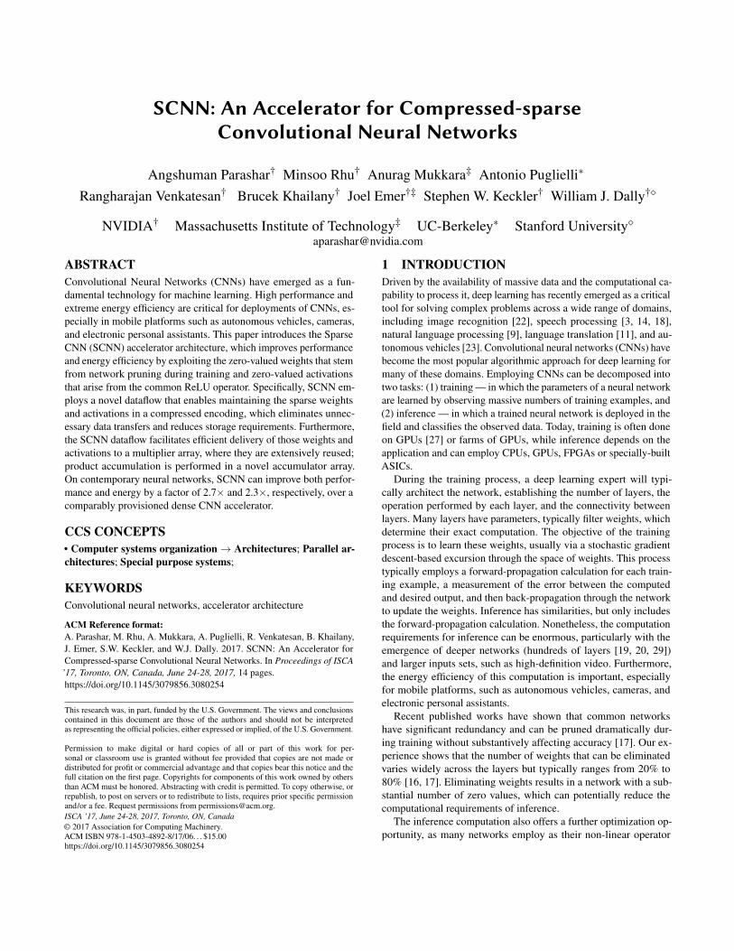
Figure 2: CNN computations and parameters.

these architectures are also able to partially elide inner-buffer ac-cesses for weights if those weights were only to be multiplied with azero-valued activation. Conversely, the Cambricon-X [34] architec-ture exploits sparsity by compressing the pruned weights, skippingcomputation cycles for zero-valued weights, but it still suffers fromwasted computation cycles when the non-zero weight is to be multi-plied with zero-valued activations.

In addition to the different approaches of exploiting sparsity,these architectures also employ distinct dataflows [7] to executea sparse convolutional layer. The most relevant distinction amongthese architectures’ dataflows is how the innermost computationdatapath exploits spatial reuse and sparsity patterns. Eyeriss uses arow-stationary dataflow, multicasting weights and activations acrossmultiple scalar processing elements (PEs), with each PE indepen-dently performing zero-activation detection. Cnvlutin multiplies asingle scalar non-zero activation across a vector of weights (orga-nized by output-channel), and then reduces these output vectorsacross different input-channels. Cambricon-X fetches activation vec-tors across input-channels based on non-zero weight vectors andcomputes their dot product, including unnecessary work for zero-valued elements of the activation vector.

SCNN’s objective is to exploit sparseness in both activationsand pruned weights to eliminate as many computation cycles anddata movement and storage operations as possible. SCNN employsa dense encoding of both sparse weights and activations so thatonly non-zero data values are retrieved from DRAM and on-chipbuffers. Unfortunately, orchestrating a dataflow to deliver thesesparse datasets to an array of multipliers while maximizing datareuse and multiplier utilization is non-trivial. Instead of coercingany of the previously proposed dataflows to suit our purpose, weemploy a novel Cartesian product dataflow that exploits both weightand activation reuse while delivering only non-zero weights andactivations to the multipliers. This dataflow performs an all-to-allmultiply of non-zero weight and activation vector elements that canavoid any arithmetic based on zero-valued operands and achieve fullmultiplier utilization in steady-state.

3 SCNN DATAFLOWWhile the inner core of the dataflow in SCNN is based on a spatialCartesian product, the complete dataflow requires a deep nestedloop structure, mapped both spatially and temporally across mul-tiple processing elements. We call the full dataflow PlanarTiled-InputStationary-CartesianProduct-sparse, or PT-IS-CP-sparse. This

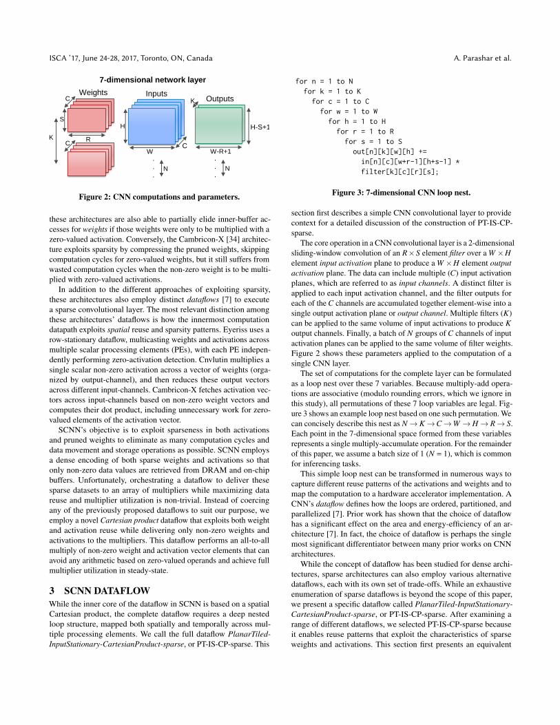
for n = 1 to Nfor k = 1 to K

for c = 1 to Cfor w = 1 to W

for h = 1 to Hfor r = 1 to R

for s = 1 to Sout[n][k][w][h] +=

in[n][c][w+r-1][h+s-1] *filter[k][c][r][s];

Figure 3: 7-dimensional CNN loop nest.

section first describes a simple CNN convolutional layer to providecontext for a detailed discussion of the construction of PT-IS-CP-sparse.

The core operation in a CNN convolutional layer is a 2-dimensionalsliding-window convolution of an R×S element filter over a W ×Helement input activation plane to produce a W ×H element outputactivation plane. The data can include multiple (C) input activationplanes, which are referred to as input channels. A distinct filter isapplied to each input activation channel, and the filter outputs foreach of the C channels are accumulated together element-wise into asingle output activation plane or output channel. Multiple filters (K)can be applied to the same volume of input activations to produce Koutput channels. Finally, a batch of N groups of C channels of inputactivation planes can be applied to the same volume of filter weights.Figure 2 shows these parameters applied to the computation of asingle CNN layer.

The set of computations for the complete layer can be formulatedas a loop nest over these 7 variables. Because multiply-add opera-tions are associative (modulo rounding errors, which we ignore inthis study), all permutations of these 7 loop variables are legal. Fig-ure 3 shows an example loop nest based on one such permutation. Wecan concisely describe this nest as N → K →C →W → H → R → S.Each point in the 7-dimensional space formed from these variablesrepresents a single multiply-accumulate operation. For the remainderof this paper, we assume a batch size of 1 (N = 1), which is commonfor inferencing tasks.

This simple loop nest can be transformed in numerous ways tocapture different reuse patterns of the activations and weights and tomap the computation to a hardware accelerator implementation. ACNN’s dataflow defines how the loops are ordered, partitioned, andparallelized [7]. Prior work has shown that the choice of dataflowhas a significant effect on the area and energy-efficiency of an ar-chitecture [7]. In fact, the choice of dataflow is perhaps the singlemost significant differentiator between many prior works on CNNarchitectures.

While the concept of dataflow has been studied for dense archi-tectures, sparse architectures can also employ various alternativedataflows, each with its own set of trade-offs. While an exhaustiveenumeration of sparse dataflows is beyond the scope of this paper,we present a specific dataflow called PlanarTiled-InputStationary-CartesianProduct-sparse, or PT-IS-CP-sparse. After examining arange of different dataflows, we selected PT-IS-CP-sparse becauseit enables reuse patterns that exploit the characteristics of sparseweights and activations. This section first presents an equivalent

SCNN ISCA ’17, June 24-28, 2017, Toronto, ON, Canada

dense dataflow (PT-IS-CP-dense) to explain the decomposition ofthe computations and then adds the specific features for PT-IS-CP-sparse.

3.1 The PT-IS-CP-dense DataflowSingle-multiplier temporal dataflow. The IS term in PT-IS-CP-dense describes the temporal component of the dataflow. First, con-sider the operation of a scalar processing element (PE) with a singlemultiply-accumulate unit. We employ an input-stationary (IS) com-putation order in which an input activation is held stationary atthe computation units as it is multiplied by all of the filter weightsneeded to make all of its contributions to each of the the K outputchannels (a K ×R×S sub-volume). Thus each input activation willcontribute to a volume of K ×W ×H output activations. This ordermaximizes the reuse of the input activations, while paying a costto stream the weights to the computation units. Accommodatingmultiple input channels (C) adds an additional outer loop and resultsin the loop nest C →W → H → K → R → S.

The PT-IS-CP-dense dataflow requires input buffers for weightsand input activations, and an accumulator buffer to store the partialsums of the output activations. The accumulator buffer must performa read-add-write operation for every access to a previously-writtenindex. We call this accumulator buffer along with the attached adderan accumulation unit.

One of the objectives of the SCNN architecture is to maximize op-portunities to store compressed activations on-die between networklayers. This requires a moderately large input buffer, which can beenergy-expensive to access. The input-stationary temporal loop nestamortizes the energy cost of accessing the input buffer over multipleweight and accumulator buffer accesses. More precisely, the registerin which the stationary input is held over K ×R×S iterations servesas an inner buffer that filters accesses to the larger input buffer.

Unfortunately, the stationarity of input activations comes at thecost of more streaming accesses to the weights and to the partialsums in the accumulator buffer. Blocking the weights and partialsums in the output channel (K) dimension can increase reuse of thesedata structures and improve energy efficiency. We therefore factorthe K output channels into K/Kc output-channel groups of sizeKc, and only store weights and outputs for a single output-channelgroup at a time inside the weight and accumulator buffers. Thus thesub-volumes that are housed in buffers at the computation unit are:

• Weights: C×Kc ×R×S• Inputs: C×W ×H• Partial Sums: Kc ×W ×H

An outer loop over all the K/Kc output-channel groups resultsin the complete loop nest K/Kc → C → W → H → Kc → R → S.Each iteration of this outer loop will require the weight buffer to berefilled and the accumulator buffer to be drained and cleared, whilethe contents of the input buffer will be fully reused because the sameinput activations are used across all output channels.

Intra-PE parallelism. The CP term in PT-IS-CP-dense describeshow parallelism of many multipliers within a PE can be exploitedwhile maximizing spatial reuse. A vector of F filter-weights fetchedfrom the weight buffer and a vector of I inputs fetched from theinput activation buffer are delivered to an array of F×I multipliers tocompute a full Cartesian product (CP) of output partial-sums. This

all-to-all operation has two useful properties. First, each fetchedweight is reused (via wire-based multicast) over all I activations;each activation is reused over all F weights. Second, each productyields a useful partial sum such that no extraneous fetches or compu-tations are performed. PT-IS-CP-sparse will exploit these same prop-erties to make computation efficient on compressed-sparse weightsand input activations.

The multiplier outputs are sent to the accumulation unit, whichupdates the partial sums of the output activation. Each multiplieroutput is accumulated with a partial sum at the matching outputcoordinates in the output activation space. These coordinates arecomputed in parallel with the multiplications. The accumulation unitmust employ at least F×I adders to match the throughput of themultipliers.

Inter-PE parallelism. Finally, the PT term in PT-IS-CP-densedescribes how to scale beyond the practical limits of multiplier countand buffer sizes within a PE. We employ a spatial tiling strategy tospread the work across an array of PEs so that each PE can operateindependently. The W×H element activation plane is partitioned intosmaller Wt×Ht element planar tiles (PT) that are distributed acrossthe PEs. Each tile extends fully into the input-channel dimensionC, resulting in an input-activation volume of C×Wt×Ht assigned toeach PE. Weights are broadcast to the PEs, and each PE operates onits own subset of the input and output activation space.

Unfortunately, strictly partitioning both input and output activa-tions into Wt ×Ht tiles does not work because the sliding-windownature of the convolution operation introduces cross-tile dependen-cies at tile edges. These data halos [13] can be resolved in one oftwo ways:

• Input halos: The input buffers at each PE are sized to beslightly larger than C×Wt ×Ht to accommodate the halos.These halo input values are replicated across adjacent PEs,but outputs are strictly private to each PE. Replicated inputvalues can be multicast when they are being fetched intothe buffers.

• Output halos: The accumulation buffers at each PE aresized to be slightly larger than Kc ×Wt ×Ht to accommo-date the halos. The halos now contain incomplete partialsums that must be communicated to neighbor PEs for ac-cumulation, which occurs at the end of computing eachoutput-channel group.

Our PT-IS-CP-dense dataflow uses output halos, though the effi-ciency difference between the two approaches is minimal.

Figure 4 shows pseudo-code for a single PE’s loop nest in the PT-IS-CP-dense dataflow, including blocking in the K dimension (A,C),fetching vectors of input activations and weights (B,D), and comput-ing the Cartesian product in parallel (E,F). X and Y coordinates forthe accumulation buffer that are either negative or greater than Wt −1and Ht −1 correspond to the locations of incomplete partial sums inthe halo regions. Communication of these halos to neighboring PEsis not shown in the figure. The Kcoord (), Xcoord (), and Y coord ()functions compute the k, x, and y coordinates of the uncompressedoutput volume using a de-linearization of the temporal loop indices aand w, the spatial loop indices i and f , and the known filter width andheight. Overall, this PT-IS-CP-dense dataflow is simply a reordered,partitioned, and parallelized version of Figure 3.

ISCA ’17, June 24-28, 2017, Toronto, ON, Canada A. Parashar et al.

BUFFER wt_buf[C][Kc*R*S/F][F];BUFFER in_buf[C][Wt*Ht/I][I];BUFFER acc_buf[Kc][Wt+R-1][Ht+S-1];BUFFER out_buf[K/Kc][Kc*Wt*Ht];

(A) for k' = 0 to K/Kc-1{

for c = 0 to C-1for a = 0 to (Wt*Ht/I)-1{

(B) in[0:I-1] = in_buf[c][a][0:I-1];(C) for w = 0 to (Kc*R*S/F)-1

{(D) wt[0:F-1] = wt_buf[c][w][0:F-1];(E) parallel_for (i = 0 to I-1) x (f = 0 to F-1)

{k = Kcoord(w,f);x = Xcoord(a,i,w,f);y = Ycoord(a,i,w,f);

(F) acc_buf[k][x][y] += in[i]*wt[f];}

}}

out_buf[k'][0:Kc*Wt*Ht-1] =acc_buf[0:Kc-1][0:Wt-1][0:Ht-1];

}

Figure 4: PT-IS-CP-dense dataflow, single-PE loop nest.

3.2 PT-IS-CP-sparse DataflowPT-IS-CP-sparse is a natural extension of PT-IS-CP-dense that ex-ploits sparsity in the weights and input activations. The dataflow isspecifically designed to operate on compressed-sparse encodings ofthe weights and input activations and produces a compressed-sparseencoding of the output activations. At a CNN layer boundary, theoutput activations of the previous layer become the input activa-tions of the next layer. While prior work has proposed a number ofcompressed-sparse representations [1, 15, 34], the specific formatused is orthogonal to the sparse architecture itself. The key feature isthat decoding a sparse format ultimately yields a non-zero data valueand an index indicating the coordinates of the value in the weight orinput activation matrices.

To facilitate easier decoding of the compressed-sparse blocks,weights are grouped into compressed-sparse blocks at the granular-ity of an output-channel group, with Kc×R×S weights encoded intoone compressed block. Likewise, input activations are encoded at thegranularity of input channels, with a block of Wt×Ht encoded intoone compressed block. At each access, the weight buffer delivers avector of F non-zero filter weights along with each of their coordi-nates within the Kc×R×S region. Similarly, the input buffer deliversa vector of I non-zero input activations along with each of theircoordinates within the Wt×Ht region. Similar to the dense dataflow,the multiplier array computes the full cross-product of F×I partialsum outputs, with no extraneous computations. Unlike a dense ar-chitecture, output coordinates are not derived from loop indices in astate machine but from the coordinates of non-zero values embeddedin the compressed format.

Even though calculating output coordinates is trivial, the multi-plier outputs are not typically contiguous as they are in PT-IS-CP-dense. Thus the F×I multiplier outputs must be scattered to discon-tiguous addresses within the Kc×Wt×Ht output range. Because any

PE

Weights

IA OA

PE

PE PE

PE PE PE

PE

DRAM

Layer

Sequ

encer

PE

Figure 5: Complete SCNN architecture.

value in the output range can be non-zero, the accumulation buffermust be kept in an uncompressed format. In fact, output activationswill probabilistically have high density even with a very low densityof weights and input activations, until they pass through a ReLUoperation.

To accommodate the needs of accumulation of sparse partialsums, we modify the monolithic Kc×Wt×Ht accumulation bufferfrom the PT-IS-CP-dense dataflow into a distributed array of smalleraccumulation buffers accessed via a scatter network which can be im-plemented as a crossbar switch. The scatter network routes an arrayof F×I partial sums to an array of A accumulator banks based on theoutput index associated with each partial sum. Taken together, thecomplete accumulator array still maps the same Kc×Wt×Ht addressrange, though the address space is now split across a distributed set ofbanks. PT-IS-CP-sparse can be implemented via small adjustmentsof Figure 4. Instead of a dense vector fetches, (B) and (D) fetch thecompressed sparse input activations and weights, respectively. Inaddition, the coordinates of the non-zero values in the compressed-sparse form of these data structures must be fetched from theirrespective buffers (not shown). Then the accumulator buffer (F)must be indexed with the computed output coordinates from thesparse weights and activations. Finally when the computation for theoutput-channel group has been completed, the accumulator buffer isdrained and compressed into the output buffer.

4 SCNN ACCELERATOR ARCHITECTURECNNs typically consist of a series of layers, including convolution,non-linear, pooling, and fully-connected. As the convolution layerstypically dominate both arithmetic and computation time, the SCNNarchitecture is optimized for efficiency on these layers. For example,on GoogLeNet, the number of multiplies in the fully connectedlayers only account for 1% of the total computation. However, SCNNalso includes dedicated logic for the simple localized non-linear andpooling layers. The non-linear layer is applied on a per-elementbasis at the end of a convolution or fully-connected layer, and isoften implemented using the ReLU operator. A pooling layer can beapplied after the ReLU layer; a typical 2×2 max pooling operatorretains the maximum value in a window of four elements, thusreducing the volume of data passed to the next layer. While fully

SCNN ISCA ’17, June 24-28, 2017, Toronto, ON, Canada

1

F

F�I

FxI multiplier array

Coordinate Computation

F

I F�I

A accumulator buffers

Neighbors

PPU Halos ReLU

Compress

IARAM (sparse)

IARAM indices

OARAM (sparse)

OARAM indices

Buffer bank

…

Buffer bank

…

…

…

I

F�I x

A

arbi

trat

ed X

BAR

Weight FIFO (sparse)

indices

DRAM

DRAM

Figure 6: SCNN PE employing the PT-IS-CP-sparse dataflow.

connected layers are similar in nature to the convolution layers, theydo require much larger weight matrices. However, recent work hasdemonstrated effective DNNs without fully connected layers [24].Section 4.3 describes further how FC layers can be processed bySCNN.

4.1 Tiled ArchitectureA full SCNN accelerator employing the PT-IS-CP-sparse dataflowof Section 3 consists of multiple SCNN processing elements (PEs)connected via simple interconnections. Figure 5 shows an array ofPEs, with each PE including channels for receiving weights andinput activations, and channels delivering output activations. ThePEs are connected to their nearest neighbors to exchange halo valuesduring the processing of each CNN layer. The PE array is drivenby a layer sequencer that orchestrates the movement of weightsand activations and is connected to a DRAM controller that canbroadcast weights to the PEs and stream activations to/from the PEs.SCNN can use an arbitrated bus as the global network to facilitatethe weight broadcasts, the point-to-point delivery of input activations(IA) from DRAM, and the return of output activations (OA) back toDRAM. The figure omits these links for simplicity.

4.2 Processing Element (PE) ArchitectureFigure 6 shows the microarchitecture of an SCNN PE, includ-ing a weight buffer, input/output activation RAMs (IARAM andOARAM), a multiplier array, a scatter crossbar, a bank of accumu-lator buffers, and a post-processing unit (PPU). To process the firstCNN layer, the layer sequencer streams a portion of the input imageinto the IARAM of each PE and broadcasts the compressed-sparseweights into the weight buffer of each PE. Upon completion of thelayer, the sparse-compressed output activation is distributed acrossthe OARAMs of the PEs. When possible, the activations are held inthe IARAMs/OARAMs and are never swapped out to DRAM. If theoutput activation volume of a layer can serve as the input activationvolume for the next layer, the IARAMs and OARAMs are logically

23

18 42

0

0

0

0 0

0

0

0 8

77

0

0

0 24

0

R

S

K

datavector

indexvector

23 18 42 2477 8

6 1 4 01 33

Figure 7: Weight compression.

swapped between the two layers’ computation sequences. Each layerof the CNN has a set of parameters that configure the controllers inthe layer sequencer, the weight FIFO, the IARAMs/OARAMs, andthe PPU to execute the required computations.

Input weights and activations. Each PE’s state machine oper-ates on the weight and input activations in the order defined bythe PT-IS-CP-sparse dataflow to produce a output-channel group ofKc ×Wt ×Ht partial sums inside the accumulation buffers. First, avector F of compressed weights and a vector I of compressed inputactivations are fetched from their respective buffers. These vectorsare distributed into the F×I multiplier array which computes a formof the Cartesian product of the vectors, i.e, every input activation ismultiplied by every weight to form a partial sum. At the same time,the indices from the sparse-compressed weights and activations areprocessed to compute the output coordinates in the dense outputactivation space.

Accumulation. The F×I products are delivered to an array of Aaccumulator banks, indexed by the output coordinates. To reducecontention among products that hash to the same accumulator bank,A is set to be larger than F×I. Our results show that A = 2×F×Isufficiently reduces accumulator bank contention. Each accumulatorbank includes adders and small set of entries for the output channelsassociated with the output-channel group being processed. The ac-cumulation buffers are double-buffered so that one set of banks canbe updated by incoming partial sums while the second set of banksare drained out by the PPU.

Post-processing. When the output-channel group is complete, thePPU performs the following tasks: (1) exchange partial sums withneighbor PEs for the halo regions at the boundary of the PE’s outputactivations, (2) apply the non-linear activation (e.g. ReLU), pooling,and dropout functions, and (3) compress the output activations intothe compressed-sparse form and write them into the OARAM. Asidefrom the neighbor halo exchange, these operations are confined tothe data values produced locally by the PE.

Compression. To compress the weights and activations, we usevariants of previously proposed compressed sparse matrix represen-tations [15, 33]. Figure 7 shows an example of SCNN’s compressed-sparse encoding for R = S = 3 and K = 2 with 6 non-zero elements.The encoding includes a data vector consisting of the non-zero values

ISCA ’17, June 24-28, 2017, Toronto, ON, Canada A. Parashar et al.

and an index vector that includes the number of non-zero values fol-lowed by the number of zeros before each value. The 3-dimensionalR×S×K volume is effectively linearized, enabling full compressionacross the dimension transitions. The activations are encoded in asimilar fashion, but across the H×W×C dimensions. As the activa-tions are divided among the PEs, each tile of compressed activationsis actually Ht×Wt×C.

We use four bits per index to allow for up to 15 zeros to appearbetween any two non-zero elements. Non-zero elements that arefurther apart can have a zero-value placeholder without incurringany noticeable degradation in compression efficiency. The original(dense) coordinates of the weights and activations are recomputed bykeeping a running sum of the number of zero and non-zero elementsand the dividing by the appropriate dimension. Determining thecoordinates in the accumulator buffer for each multiplier outputrequires reconstructing the coordinates from index vectors for Fand I and combining them with the coordinates of the portion ofthe output activation space currently being processed. The encodingscheme can be enhanced with optimizations such as rounding up thedimension of each weight filter to a power of two to make divisioneasier or using the four index bits per entry to encode a non-uniformnumber of zeros. While these optimizations would increase densitysomewhat, they do not substantively affect the SCNN architectureor our observed results.

4.3 Fully-connected LayersWhile our Cartesian product-based SCNN dataflow dramaticallyimproves its efficiency at the convolutional layers, it does imposesome challenges when handling fully-connected layers. Concretely,unlike a convolution filter, an individual weight connection in a fully-connected layer is not reused across multiple input activations. Thus,the Cartesian product approach of SCNN does not automaticallyalign non-zero weights and activations that must be multiplied. Asa result, the SCNN 4×4 multiplier array can only operate at a peakrate of 4 multiplies per cycles (25% of peak throughput) because the4 input activations and 4 weights can produce only 4 useful products.Another challenge with fully-connected layers is aligning the sparseweights and the sparse activations so that the appropriate non-zerovalues are delivered into the multiplier array at the same time. TheSCNN’s logic for processing the activation and weight indices can bereused to determine the alignment, but some additional multiplexinghardware would be required to move the non-zero weights intoposition.

While the loss of average throughput at the fully-connected layerswould make SCNN unattractive for networks that are dominatedby fully-connected layers, state-of-the-art CNNs for image classi-fication, detection, and segmentation are primarily dominated bythe convolutional layers; in the networks we used in our study, thefully-connected layers accounted for only 8%, 1%, and 2% of themultiplication operations in AlexNet, GoogLeNet, and VGGNet,respectively. In addition, networks for computer vision are decreas-ing their reliance of fully-connected networks and in fact, recentnetworks eliminate these layers completely [24]. Furthermore, thefully-connected layers are generally memory-bandwidth limited asthey spend most of their execution time delivering network weightsfrom DRAM. While SCNN’s noticeable throughput reduction on

Table 3: SCNN design parameters.

PE Parameter ValueMultiplier width 16 bitsAccumulator width 24 bitsIARAM/OARAM (each) 10KBWeight FIFO 50 entries (500 B)Multiply array (F×I) 4×4Accumulator banks 32Accumulator bank entries 32

SCNN Parameter Value# PEs 64# Multipliers 1,024IARAM + OARAM data 1MBIARAM + OARAM indices 0.2MB

fully-connected layers is not ideal, it is not a significant performancelimiter for these memory-hungry layers. We argue that systems de-siring optimal efficiency for both convolution and fully-connectedlayers should consider employing both SCNN and an architecturesuch as EIE that is optimized for fully-connected layers [15].

4.4 Temporal Tiling for Large ModelsSCNN compresses weights and activations to reduce both arithmeticoperations and data movement. Ideally, the degree of compressionand the capacity of the IARAMs and OARAMs are large enough sothat the activations are never evicted to outer layers of the memoryhierarchy. While we size our activation RAMs to capture the capacityrequirements of nearly all of the layers in the networks we examined,a few layers of VGGNet require activations to be saved to andrestored from DRAM. Like other accelerator architectures, SCNNcan temporally tile the activation space so that the collection of PEsoperate on a sub-volume of the activations at a time. This temporaltiling can be applied in addition to the spatial tiling that SCNNalready employs to partition the activation volume across the PEs.

While a temporally tiled convolution layer still broadcasts weightsto all of the PEs, the input activation planes are partitioned intocoarse-grained tiles (across all channels) that each fit into the totalIARAM capacity of the accelerator. The output activation tile isoffloaded to DRAM and then reloaded into the IARAM when thedata is needed as the input activation to the next layer. This type oftiling leads to a small halo at the edge of each input activation tile,resulting in a few additional input activation fetches from DRAM.The temporally tiled PT-IS-CP-sparse dataflow still exploits the reuseof each input activation value from the IARAM R×S×Kc times.

In the networks we analyzed, only 9 of the 72 total layers failto fit entirely within the IARAM/OARAM structures, with all ofthem coming from VGGNet. Our analysis shows that for both denseand sparse architectures, the DRAM accesses for one temporal tilecan be hidden by pipelining them in tandem with the computationof another tile. Our nominal DRAM bandwidth configuration of 50GB/s provides ample bandwidth to absorb the additional activationtraffic. Only when DRAM bandwidth drops to around 4 GB/s doesperformance degrade. On these 9 layers, the per-layer energy penaltyof activation data transfer ranges from 5–62%, with a mean of 18%.This overhead is fairly low and will be born by all CNN architectureswith similar levels of on-chip RAM for activations; overheads will

SCNN ISCA ’17, June 24-28, 2017, Toronto, ON, Canada

Table 4: SCNN PE area breakdown.

PE Component Size Area (mm2)

IARAM + OARAM 20 KB 0.031Weight FIFO 0.5 KB 0.004Multiplier array 16 ALUs 0.008Scatter network 16×32 crossbar 0.026Accumulator buffers 6 KB 0.036Other — 0.019Total — 0.123

Accelerator total 64 PEs 7.9

be higher for accelerators that do not compress activations. While thetiling approach is attractive, we expect some low power deploymentscenarios to motivate neural networks designers to size them so thatthey fit completely in the on-chip SRAM capacity provided by theaccelerator implementation.

4.5 SCNN Architecture ConfigurationWhile the SCNN architecture can be scaled across a number ofdimensions, Table 3 lists the key parameters of the SCNN designwe explore in this paper. The design employs an 8×8 array of PEs,each with a 4×4 multiplier array, and an accumulator buffer with32 banks. We chose a design point of 1,024 multipliers to matchthe expected computation throughput required to process HD videoin real-time at acceptable frame rates. The IARAM and OARAMare sized so that the sparse activations of AlexNet and GoogLeNetcan fit entirely within these RAMs so that activations need not spillto DRAM. The weight FIFO and the activation RAMs each carrya 4-bit overhead for each 16-bit value to encode the coordinates inthe compressed-sparse format. In total, the SCNN design includesa total of 1,024 multipliers and 1MB of activation RAM. At thesynthesized clock speed of the PE of slightly more than 1 GHz ina 16nm technology, this design achieves a peak throughput of 2Tera-ops (16-bit multiplies plus 24-bit adds).

Area Analysis. To prototype the SCNN architecture, we designedan SCNN PE in synthesizable SystemC and then used the Catapulthigh-level synthesis (HLS) tool [25, 26] to generate Verilog RTL.During this step, we used HLS design constraints to optimize the de-sign by mapping different memory structures to synchronous RAMsand latch arrays and pipelining the design to achieve full throughput.We then used Synopsys Design Compiler to perform placement-aware logic synthesis and obtain post-synthesis area estimates in aTSMC 16nm FinFET technology. Table 4 summarizes the area of themajor structures of the SCNN PE. A significant fraction of the PEarea is contributed by memories (IARAM, OARAM, accumulatorbuffers), which consume 57% of the PE area, while the multiplierarray only consumes 6%. IARAM and OARAM are large in sizeand consume 25% of the PE area. Accumulator buffers, thoughsmaller in size compared to IARAM/OARAM, are heavily banked(32 banks), contributing to their large area.

5 EXPERIMENTAL METHODOLOGYCNN performance and power measurements. To model the per-formance of the SCNN architecture, we rely primarily on a custom-built cycle-level simulator. This simulator is parameterizable across

Table 5: CNN accelerator configurations.

# PEs # MULs SRAM Area (mm2)

DCNN 64 1,024 2MB 5.9DCNN-opt 64 1,024 2MB 5.9

SCNN 64 1,024 1MB 7.9

dimensions including number of processing element (PE) tiles, RAMcapacity, multiplier array dimensions (F and I), and accumulatorbuffers (A). The SCNN simulator is driven by the pruned weightsand sparse input activation maps extracted from the Caffe Pythoninterface (pycaffe) [4] and executes each layers of the network oneat a time. As a result, the simulator precisely captures the effects ofthe sparsity of the data and its effect on load balancing within theSCNN architecture.

We also developed TimeLoop, a detailed analytical model forCNN accelerators to enable an exploration of the design space ofdense and sparse architectures. TimeLoop can model a wide rangeof dataflows, including PT-IS-CP-sparse and PT-IS-CP-dense, aswell as the dataflows described in Table 2. Architecture parametersto TimeLoop include the memory hierarchy configuration (buffersize and location), ALU count and partitioning, and dense/sparsehardware support. TimeLoop also includes DRAM bandwidth andenergy models for off-chip accesses. TimeLoop analyzes the in-put data parameters, the architecture, and the dataflows, and thencomputes (1) the number of cycles to process the layer based ona bottleneck analysis, and (2) the counts of ALU operations andaccesses to different buffers in the memory hierarchy. We apply anenergy model to the TimeLoop events derived from the synthesismodeling to compute the overall energy required to execute the layer.TimeLoop also computes the overall area of the accelerator based onthe inputs from the synthesis modeling. For SCNN, the area modelincludes all of the elements from the synthesizable SystemC imple-mentation. For dense architectures, area is computed using area ofthe major structures (RAMs, ALUs, and interconnect) derived fromthe SystemC modeling.

Architecture configurations. Table 5 summarizes the major ac-celerator configurations that we explore, including both dense andsparse accelerators. All of the accelerators employ the same num-ber of multipliers so that we can compare the performance of theaccelerators with the same computational resources. The dense DCNNaccelerator operates solely on dense weights and activations andemploys a dot-product dataflow called PT-IS-DP-dense. Dot prod-ucts are usually efficient for dense accelerators because of reducedaccumulation-buffer accesses, although this comes at the cost ofreduced spatial reuse of weights and input activations. The opti-mized DCNN-opt architectures have the same configuration as DCNNbut employ two optimizations: (1) compression/decompression ofactivations as they are transferred out of/into DRAM, and (2) mul-tiply ALU gating to save energy when a multiplier input is zero.The DCNN architectures are configured with 2MB of SRAM for hold-ing inter-layer activations, and can hold all of them for AlexNetand GoogLeNet. The SCNN configuration matches the architecturedescribed in Section 4, and includes a total of 1MB of IARAM+ OARAM. Because the activations are compressed, this capacityenables all of the activation data for the two networks to be held on

ISCA ’17, June 24-28, 2017, Toronto, ON, Canada A. Parashar et al.

chip, without requiring DRAM transfers for activations. The largerVGGNet requires the activation data to be transferred in and out ofDRAM. The last column of the table lists the area required for eachaccelerator; for simplicity, we total only the area for the PE arrayand SRAM banks, and omit any area for wiring among the PEs. Asthe interconnect bandwidth requirements for SCNN are less than fordense architectures due to the compression, including interconnectarea for both dense and sparse architectures would close the areagap somewhat between the two. While SCNN has smaller activa-tion RAM capacity, its larger size is due to the banked accumulatorbuffers, as described in Section 4.

Benchmarks. As described in Section 2, we use AlexNet andGoogLeNet for the bulk of our experiments. For GoogLeNet, weprimarily focus on the convolutional layers that are within the in-ception modules [31]. VGGNet is known to be over-parameterized,which results in an excessively large amount of inter-layer activationdata (6 MB or about 4× the largest GoogLeNet layer). Nonetheless,we use VGGNet as a proxy for large input data (such has high-resolution images) to explore the implications of coarse-grainedtemporal tiling on accelerator architectures. We leverage two differ-ent types of benchmarks to evaluate SCNN’s efficiency. First, wedeveloped synthetic network models where we can adjust the degreeof sparsity of both weights and activations. These synthetic modelsare used to explore the sensitivity of the architectures to sparsityparameters (detailed in Section 6.1.). Second, we generate the actualsparse network models using the CNN pruning algorithm proposedby Han et al. [17], which we employ in cycle-level performancesimulation. The pruned models have been retrained to achieve thesame level of classification accuracy provided by the dense model,and we use this pruned model to obtain the post-ReLU activationmaps to feed it into our performance simulator.

6 EVALUATIONThis section first evaluates the sensitivity of SCNN to the sparsenessof weights and activations using a synthetic CNN benchmark. Wethen measure the performance and energy-efficiency of SCNN versusa dense CNN accelerator, using AlexNet, GoogLeNet, and VGGNet.For brevity, all the inception modules in GoogLeNet are denoted asIC_id in all of the figures discussed in this section.

6.1 Sensitivity to CNN SparsityWe first compare the performance and energy-efficiency of the SCNN,DCNN, and DCNN-opt architectures as we artificially sweep the weightand activation densities in GoogLeNet’s layers from 100% (fullydense) down to 10%. The X-axis of Figure 8 simultaneously scalesboth weight and activation density. The 0.5/0.5 point correspondsto 50% weight density, 50% activation density, and 25% of themultiplication operations relative to the fully-dense 1.0/1.0 point.Figure 8a shows that at full density, SCNN only achieves about 79%of the performance of DCNN/DCNN-opt1 because of SCNN’s dataflowis more susceptible to certain multiplier underutilization effects thanDCNN’s dot-product dataflow. As density decreases to about 0.85/0.85,SCNN starts to perform better than DCNN, ultimately reaching a 24×improvement at the sparsest evaluated point with a density of 0.1/0.1.

1DCNN-opt performance is identical to DCNN because it only optimizes for energy.

0

0.2

0.4

0.6

0.8

1

1.2

1.4

0.1/0.1 0.2/0.2 0.3/0.3 0.4/0.4 0.5/0.5 0.6/0.6 0.7/0.7 0.8/0.8 0.9/0.9 1.0/1.0

Late

ncy

(cy

cle

s)

Weight / Activation Density

DCNN/DCNN-opt SCNN

(a) Performance

0

0.2

0.4

0.6

0.8

1

1.2

1.4

0.1/0.1 0.2/0.2 0.3/0.3 0.4/0.4 0.5/0.5 0.6/0.6 0.7/0.7 0.8/0.8 0.9/0.9 1.0/1.0

Ene

rgy

Weight / Activation Density

DCNN DCNN-opt SCNN

(b) Energy

Figure 8: GoogLeNet performance and energy versus density.

Figure 8b first shows that DCNN-opt’s energy optimizations ofzero gating and DRAM traffic compression enable it to be better thanDCNN at every level of density. These energy optimizations are sur-prisingly effective despite their minimal effect on the design of theaccelerator. At full density, SCNN consumes 33% more energy thaneither dense architecture due to the overheads of storing and main-taining the sparse data structures. SCNN becomes more efficient thanDCNN at about 0.83/0.83 density and more efficient than DCNN-optat 0.6/0.6 density. At the sparsest evaluated point of 0.1/0.1 density,SCNN consumes 6% of the energy of DCNN and 23% of the energyof DCNN-opt. Given the density measurements of the networks inFigure 1, we expect SCNN to (a) significantly outperform the densearchitectures on nearly all the layers of the networks we examined,(b) surpass the energy efficiency of DCNN on a majority of layers, and(c) stay roughly competitive with the energy-efficiency of DCNN-optacross most layers.

6.2 SCNN Performance and EnergyPerformance. We compare the performance of SCNN to the base-line dense DCNN accelerator and to an oracular SCNN design(SCNN(oracle)) that represents an upper bound on performance.The performance of SCNN(oracle) is derived by dividing the num-ber of multiplication operations required for a Cartesian product-based convolution (Section 3) by 1,024, the number of multipliersin the architectures we examine. Figure 9 summarizes the speedupsoffered by SCNN versus a dense CNN accelerator. Overall, SCNNconsistently outperforms the DCNN design across all the layers ofAlexNet, GoogLeNet, and VGGNet, achieving an average 2.37×,2.19×, and 3.52× network-wide performance improvement, respec-tively.

SCNN ISCA ’17, June 24-28, 2017, Toronto, ON, Canada

0

2

4

6

8

10

12

conv1 conv2 conv3 conv4 conv5 all

Per-layer Network

Speedup

DCNN/DCNN-opt SCNN SCNN (oracle)

(a) AlexNet

0

2

4

6

8

10

12

14

IC_3a IC_3b IC_4a IC_4b IC_4c IC_4d IC_4e IC_5a IC_5b all

Per-layer Network

Speedup

DCNN/DCNN-opt SCNN SCNN (oracle)

(b) GoogLeNet

0

3

6

9

12

15

con

v1_1

con

v1_2

con

v2_1

con

v2_2

con

v3_1

con

v3_2

con

v3_3

con

v4_1

con

v4_2

con

v4_3

con

v5_1

con

v5_2

con

v5_3 al

l

Per-layer Network

Speedup

DCNN/DCNN-opt SCNN SCNN (oracle)

(c) VGGNet

Figure 9: SCNN performance comparison.

The performance gap between SCNN versus SCNN(oracle) widensin later layers of the network, i.e., the rightmost layers on the x-axisof Figure 9. SCNN suffers from two forms of inefficiency that causethis gap. First, the working set allocated to each PE tends to besmaller in the later layers (e.g., IC_5b) than in the earlier layers(e.g., IC_3a). As a result, assigning enough non-zero activations andweights in the later layers to fully utilize a PE’s multiplier arraybecomes difficult. In other words, SCNN can suffer from intra-PEfragmentation when layers do not have enough useful work to fullypopulate the vectorized arithmetic units.

The second source of inefficiency stems from the way the PT-IS-CP-sparse dataflow partitions work across the array of PEs, whichcould lead to load imbalance among the PEs. Load imbalance resultsin under-utilization because the work corresponding to the nextoutput-channel group Kc+1 can only start after the PEs complete thecurrent output-channel group Kc. The PEs effectively perform aninter-PE synchronization barrier at the boundaries of output-channelgroups which can cause early-finishing PEs to idle while waiting forlaggards.

Figure 10 quantitatively demonstrates the intra-PE fragmentationin the multiplier arrays. Fragmentation is severe in the last twoinception modules of GoogLeNet, with average multiplier utilizationat less than 20%. In this layer, three out of the six convolutional sub-layers within the inception module have a filter size of 1×1, resulting

0

0.2

0.4

0.6

0.8

1

0

0.2

0.4

0.6

0.8

1

conv1 conv2 conv3 conv4 conv5

Avg

. PE

idle

cyc

les

Avg

. mu

ltip

lier

uti

l.

Multiplier util.

PE idle cycles

(a) AlexNet

0

0.2

0.4

0.6

0.8

1

0

0.2

0.4

0.6

0.8

1

IC_3a IC_3b IC_4a IC_4b IC_4c IC_4d IC_4e IC_5a IC_5b

Avg

. PE

idle

cyc

les

Avg

. mu

ltip

lier

uti

l.

mul_util

idle_cycles

(b) GoogLeNet

0

0.2

0.4

0.6

0.8

1

0

0.2

0.4

0.6

0.8

1

Avg

. PE

idle

cyc

les

Avg

. mu

ltip

lier

uti

l.

mul_utilidle_cycles

(c) VGGNet

Figure 10: Average multiplier array utilization (left-axis) andthe average fraction of time PEs are stalled on a global barrier(right-axis), set at the boundaries of output channel groups.

in a maximum of 8 non-zero weights within an output-channel groupwith a Kc value of 8. Nonetheless, later layers generally account fora small portion of the overall execution time as the input activationvolume (i.e., H×W×C) gradually diminishes across the layers.

The right y-axis of Figure 10 demonstrates the effect of loadimbalance across the PEs by showing the fraction of cycles spentwaiting at an inter-PE barrier. Although the inter-PE global barriersand intra-PE fragmentation prevents SCNN from reaching similarspeedups offered by SCNN(oracle), it still provides an average2.7× network-wide performance boost over DCNN across the threeCNNs we examined.

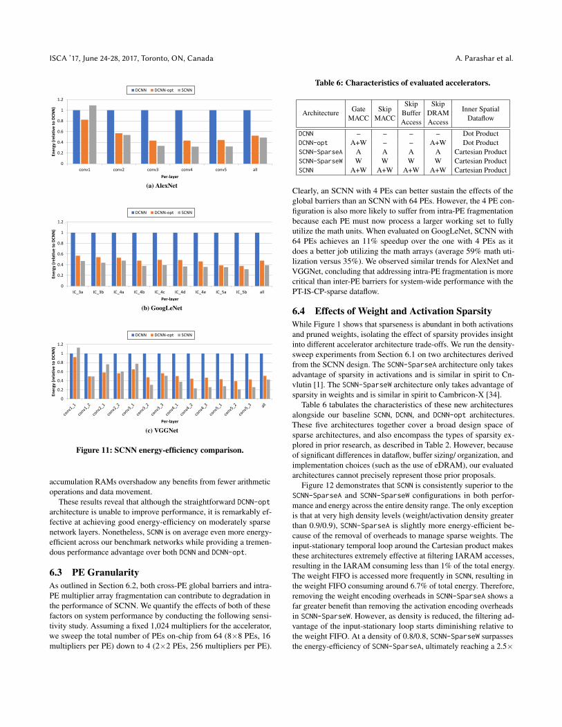
Energy-efficiency. Figure 11 compares the energy of the threeaccelerator architectures across the layers of the three networks. Onaverage, DCNN-opt improves energy-efficiency by 2.0× over DCNN,while SCNN improves efficiency by 2.3× . SCNN’s effectiveness varieswidely across layers depending on the layer density, ranging from0.89× to 4.7× improvement over DCNN and 0.76× to 1.9× improve-ment over DCNN-opt. Input layers such as VGGNet_conv1_1 andAlexNet_conv1 usually present a challenge for sparse architecturesbecause of their 100% input activation density. In such cases, theoverheads of SCNN’s structures such as the crossbar and distributed

ISCA ’17, June 24-28, 2017, Toronto, ON, Canada A. Parashar et al.

0

0.2

0.4

0.6

0.8

1

1.2

conv1 conv2 conv3 conv4 conv5 all

Ene

rgy

(re

lati

ve t

o D

CN

N)

Per-layer

DCNN DCNN-opt SCNN

(a) AlexNet

0

0.2

0.4

0.6

0.8

1

1.2

IC_3a IC_3b IC_4a IC_4b IC_4c IC_4d IC_4e IC_5a IC_5b all

Ene

rgy

(re

lati

ve t

o D

CN

N)

Per-layer

DCNN DCNN-opt SCNN

(b) GoogLeNet

0

0.2

0.4

0.6

0.8

1

1.2

Ene

rgy

(re

lati

ve t

o D

CN

N)

Per-layer

DCNN DCNN-opt SCNN

(c) VGGNet

Figure 11: SCNN energy-efficiency comparison.

accumulation RAMs overshadow any benefits from fewer arithmeticoperations and data movement.

These results reveal that although the straightforward DCNN-optarchitecture is unable to improve performance, it is remarkably ef-fective at achieving good energy-efficiency on moderately sparsenetwork layers. Nonetheless, SCNN is on average even more energy-efficient across our benchmark networks while providing a tremen-dous performance advantage over both DCNN and DCNN-opt.

6.3 PE GranularityAs outlined in Section 6.2, both cross-PE global barriers and intra-PE multiplier array fragmentation can contribute to degradation inthe performance of SCNN. We quantify the effects of both of thesefactors on system performance by conducting the following sensi-tivity study. Assuming a fixed 1,024 multipliers for the accelerator,we sweep the total number of PEs on-chip from 64 (8×8 PEs, 16multipliers per PE) down to 4 (2×2 PEs, 256 multipliers per PE).

Table 6: Characteristics of evaluated accelerators.

GateMACC

SkipMACC

Skip SkipInner Spatial

DataflowArchitecture Buffer DRAM

Access Access

DCNN – – – – Dot ProductDCNN-opt A+W – – A+W Dot ProductSCNN-SparseA A A A A Cartesian ProductSCNN-SparseW W W W W Cartesian ProductSCNN A+W A+W A+W A+W Cartesian Product

Clearly, an SCNN with 4 PEs can better sustain the effects of theglobal barriers than an SCNN with 64 PEs. However, the 4 PE con-figuration is also more likely to suffer from intra-PE fragmentationbecause each PE must now process a larger working set to fullyutilize the math units. When evaluated on GoogLeNet, SCNN with64 PEs achieves an 11% speedup over the one with 4 PEs as itdoes a better job utilizing the math arrays (average 59% math uti-lization versus 35%). We observed similar trends for AlexNet andVGGNet, concluding that addressing intra-PE fragmentation is morecritical than inter-PE barriers for system-wide performance with thePT-IS-CP-sparse dataflow.

6.4 Effects of Weight and Activation SparsityWhile Figure 1 shows that sparseness is abundant in both activationsand pruned weights, isolating the effect of sparsity provides insightinto different accelerator architecture trade-offs. We run the density-sweep experiments from Section 6.1 on two architectures derivedfrom the SCNN design. The SCNN-SparseA architecture only takesadvantage of sparsity in activations and is similar in spirit to Cn-vlutin [1]. The SCNN-SparseW architecture only takes advantage ofsparsity in weights and is similar in spirit to Cambricon-X [34].

Table 6 tabulates the characteristics of these new architecturesalongside our baseline SCNN, DCNN, and DCNN-opt architectures.These five architectures together cover a broad design space ofsparse architectures, and also encompass the types of sparsity ex-plored in prior research, as described in Table 2. However, becauseof significant differences in dataflow, buffer sizing/ organization, andimplementation choices (such as the use of eDRAM), our evaluatedarchitectures cannot precisely represent those prior proposals.

Figure 12 demonstrates that SCNN is consistently superior to theSCNN-SparseA and SCNN-SparseW configurations in both perfor-mance and energy across the entire density range. The only exceptionis that at very high density levels (weight/activation density greaterthan 0.9/0.9), SCNN-SparseA is slightly more energy-efficient be-cause of the removal of overheads to manage sparse weights. Theinput-stationary temporal loop around the Cartesian product makesthese architectures extremely effective at filtering IARAM accesses,resulting in the IARAM consuming less than 1% of the total energy.The weight FIFO is accessed more frequently in SCNN, resulting inthe weight FIFO consuming around 6.7% of total energy. Therefore,removing the weight encoding overheads in SCNN-SparseA shows afar greater benefit than removing the activation encoding overheadsin SCNN-SparseW. However, as density is reduced, the filtering ad-vantage of the input-stationary loop starts diminishing relative tothe weight FIFO. At a density of 0.8/0.8, SCNN-SparseW surpassesthe energy-efficiency of SCNN-SparseA, ultimately reaching a 2.5×

SCNN ISCA ’17, June 24-28, 2017, Toronto, ON, Canada

0

0.2

0.4

0.6

0.8

1

1.2

1.4

0.1/0.1 0.2/0.2 0.3/0.3 0.4/0.4 0.5/0.5 0.6/0.6 0.7/0.7 0.8/0.8 0.9/0.9 1.0/1.0

Late

ncy

(cy

cle

s)

Weight / Activation Density

DCNN/DCNN-opt SCNN-SparseWeights SCNN-SparseActivations SCNN

(a) Performance

0

0.2

0.4

0.6

0.8

1

1.2

1.4

0.1/0.1 0.2/0.2 0.3/0.3 0.4/0.4 0.5/0.5 0.6/0.6 0.7/0.7 0.8/0.8 0.9/0.9 1.0/1.0

Ene

rgy

Weight / Activation Density

DCNN DCNN-opt SCNN-SparseWeights SCNN-SparseActivations SCNN

(b) Energy

Figure 12: GoogLeNet performance and energy versus densityfor sparse weights, sparse activations, and both

advantage at 0.1/0.1. For a nominal density of 0.4/0.4, SCNN achievesperformances advantages of 1.7× and 2.6× over SCNN-SparseW andSCNN-SparseA, respectively; SCNN achieves energy-efficiency ad-vantages of 1.6× and 2.1× over SCNN-SparseW and SCNN-SparseA,respectively.

7 RELATED WORKPrevious efforts to exploit sparsity in CNN accelerators have focusedon reducing energy or saving time, which will invariably also saveenergy. Eliminating the multiplication when an input operand iszero is a natural way to save energy. Eyeriss [8] gates the multiplierwhen it sees an input activation of zero. Because the sparsity ofweights is not significant for non-pruned networks, Eyeriss optednot to gate the multiplier on zero weights. This gating approach willsave energy, but not execution time. Not only does SCNN obtainenergy efficiency by eliminating unnecessary multiplications, it alsoreduces execution time by eliminating the dead multiplier cyclesinherent in zero-gating approaches.

Another approach to reducing energy is to reduce data transfercosts when the data is sparse. Eyeriss uses a run length encodingscheme when transferring activations to and from DRAM. Thisapproach saves energy (and time) by reducing the number of DRAMaccesses. However because the data is kept in an expanded form inthe on-chip memory hierarchy, such architectures cannot completelyeliminate energy on the data transfers from one internal buffer toanother internal buffer or to the multipliers. Eyeriss does, however,save the energy for accessing the weight buffer when the associatedactivation is zero. SCNN also uses a compressed representation forall data coming from DRAM, but also maintains that compressedrepresentation in all the on-die buffers.

Other sparse CNN accelerator architectures do not exploit all ofthe sparsity opportunities leveraged by SCNN. For example, Cn-vlutin compresses activation values based on the ReLU operator, butit does not employ pruning to exploit weight sparsity [1]. Cambricon-X employs weight sparsity to keep only non-zero weights in itsinternal buffers [34]. However, it does not compress activation databetween DRAM and the accelerator. Nor does it keep activationsin a compressed form in the internal buffers, except in the queuesdirectly delivering activations to the multipliers. In contrast, SCNNkeeps both weights and activations in a compressed form in bothDRAM and internal buffers. This approach saves data transfer timeand energy on all data transfers and allows the chip hold largermodels for a given amount of internal storage.

Avoiding delivery of zero-valued activations or weights to themultipliers can save time by eliminating ineffectual multiplier cy-cles. Cnvlutin selects only non-zero activation values for deliveryas multiplier operands, but does occupy a multiplier with zero-valued weights. Cambricon-X can save a compute cycle for zero-valued weights, but still wastes times computing multiplications foroperands with zero-valued activations. The Deep Learning Accel-erator Core (DLAC) architecture paper mentions that it can skipcomputation on zero-valued operands to improve performance, butthe architecture does not appear to employ zero compression [32].SCNN does not deliver either zero activations or weights to themultipliers and maximally exploits opportunities of CNN sparsity.

The EIE CNN accelerator uses a compressed representation ofboth activations and weights, and only delivers non-zero operandsto the multipliers [15]. However, EIE is designed for the fully con-nected layers of a CNN model, while SCNN targets the convolutionallayers, which encompass the vast majority of the computations inCNNs [10, 24]. Finally, Alwani et al. propose to fuse adjacent layersin a dense CNN accelerator so that intermediate activations betweenlayers can be kept on chip [2]. By compressing the activations,SCNN can typically keep all of the activations on-chip, withoutrequiring a more complicated fused algorithm.

8 CONCLUSIONThis paper presents the Sparse CNN (SCNN) accelerator architec-ture for inference in convolutional neural networks. SCNN exploitssparsity in both weights and activations using the sparse planar-tiledinput-stationary Cartesian product (PT-IS-CP-sparse) dataflow. Thisapproach enables SCNN to use a novel Cartesian product-basedcomputation architecture that maximizes reuse of weights and acti-vations within a set of distributed processing elements. In addition, itallows the use of a dense compressed representation for both weightsand activations to be used through almost the entire processing flow.This allows for reduced data movement and increased on-die storagecapacity than alternatives approaches. Our results show that withequivalent area, the SCNN architecture starts to beat an energy-optimized dense architecture on energy efficiency when the weightsand activations are each less than 85% dense. On three contempo-rary networks (AlexNet, GoogLeNet, and VGGNet) SCNN achievesperformance improvements over a comparably provisioned denseCNN accelerator by a factor of 2.7×, while still being 2.3× moreenergy-efficient.

ISCA ’17, June 24-28, 2017, Toronto, ON, Canada A. Parashar et al.

REFERENCES[1] Jorge Albericio, Patrick Judd, Tayler Hetherington, Tor Aamodt, Natalie Enright

Jerger, and Andreas Moshovos. 2016. Cnvlutin: Ineffectual-Neuron-Free DeepConvolutional Neural Network Computing. In Proceedings of the InternationalSymposium on Computer Architecture (ISCA). 1–13.

[2] Manoj Alwani, Han Chen, Michael Ferdman, and Peter Milder. 2016. Fused-Layer CNN Accelerators. In Proceedings of the International Symposium onMicroarchitecture (MICRO).

[3] Dario Amodei, Rishita Anubhai, Eric Battenberg, Carl Case, Jared Casper, BryanCatanzaro, Jingdong Chen, Mike Chrzanowski, Adam Coates, Greg Diamos, ErichElsen, Jesse Engel, Linxi Fan, Christopher Fougner, Tony Han, Awni Hannun,Billy Jun, Patrick LeGresley, Libby Lin, Sharan Narang, Andrew Ng, Sherjil Ozair,Ryan Prenger, Jonathan Raiman, Sanjeev Satheesh, David Seetapun, ShubhoSengupta, Yi Wang, Zhiqian Wang, Chong Wang, Bo Xiao, Dani Yogatama, JunZhan, and Zhenyao Zhu. 2015. Deep Speech 2: End-To-End Speech Recognitionin English and Mandarin. https://arxiv.org/abs/1512.02595. (2015).

[4] Caffe 2016. Caffe. http://caffe.berkeleyvision.org. (2016).[5] Caffe 2017. Caffe Model Zoo. https://github.com/BVLC/caffe/wiki/Model-Zoo.

(2017).[6] Tianshi Chen, Zidong Du, Ninghui Sun, Jia Wang, Chengyong Wu, Yunji Chen,

and Olivier Temam. 2014. DianNao: A Small-footprint High-throughput Ac-celerator for Ubiquitous Machine-learning. In Proceedings of the InternationalConference on Architectural Support for Programming Languages and OperationSystems (ASPLOS). 269–284.

[7] Yu-Hsin Chen, Joel Emer, and Vivienne Sze. 2016. Eyeriss: A Spatial Architecturefor Energy-Efficient Dataflow for Convolutional Neural Networks. In Proceedingsof the International Symposium on Computer Architecture (ISCA). 367–379.

[8] Yu-Hsin Chen, Tushar Krishna, Joel Emer, and Vivienne Sze. 2016. Eyeriss:An Energy-efficient Reconfigurable Accelerator for Deep Convolutional NeuralNetworks. In Proceedings of the International Solid State Circuits Conference(ISSCC).

[9] Ronan Collobert, Jason Weston, Leon Bottou, Michael Karlen, KorayKavukcuoglu, and Pavel Kuksa. 2011. Natural Language Processing (Almost)From Scratch. https://arxiv.org/abs/1103.0398. (2011).

[10] Jason Cong and Bingjun Xiao. 2014. Minimizing Computation in ConvolutionalNeural Networks. In Proceedings of the International Conference on ArtificialNeural Networks (ICANN). 281–290.

[11] Gregory Diamos, Shubho Sengupta, Bryan Catanzaro, Mike Chrzanowski, AdamCoates, Erich Elsen, Jesse Engel, Awni Hannun, and Sanjeev Satheesh. 2016.Persistent RNNs: Stashing Recurrent Weights On-Chip. In Proceedings of theInternational Conference on Machine Learning (ICML).

[12] Zidong Du, Robert Fasthuber, Tianshi Chen, Paolo Ienne, Ling Li, Tao Luo,Xiaobing Feng, Yunji Chen, and Olivier Temam. 2015. ShiDianNao: ShiftingVision Processing Closer to the Sensor. In Proceedings of the InternationalSymposium on Computer Architecture (ISCA). 92–104.

[13] Mingyu Gao, Jing Pu, Xuan Yang, Mark Horowitz, and Christos Kozyrakis. 2017.TETRIS: Scalable and Efficient Neural Network Acceleration with 3D Memory.In Proceedings of the International Conference on Architectural Support forProgramming Languages and Operation Systems (ASPLOS). 751–764.

[14] Alex Graves and Jurgen Schmidhuber. 2005. Framewise Phoneme ClassificationWith Bidirectional LSTM and Other Neural Network Architectures. In NeuralNetworks.

[15] Song Han, Xingyu Liu, Huizi Mao, Jing Pu, Ardavan Pedram, Mark Horowitz,and Bill Dally. 2016. EIE: Efficient Inference Engine on Compressed DeepNeural Network. In Proceedings of the International Symposium on Computer

Architecture (ISCA). 243–254.[16] Song Han, Huizi Mao, and William J. Dally. 2015. Deep Compression: Com-

pressing Deep Neural Networks with Pruning, Trained Quantization and HuffmanCoding. https://arxiv.org/abs/1510.00149. (2015).

[17] Song Han, Jeff Pool, John Tran, and William J. Dally. 2015. Learning BothWeights and Connections for Efficient Neural Networks. In Proceedings of theInternational Conference on Neural Information Processing Systems (NIPS).1135–1143.

[18] Awni Hannun, Carl Case, Jared Casper, Bryan Catanzaro, Greg Diamos, ErichElsen, Ryan Prenger, Sanjeev Satheesh, Shubho Sengupta, Adam Coates, andAndrew Y. Ng. 2014. Deep Speech: Scaling Up End-To-End Speech Recognition.https://arxiv.org/abs/1412.5567. (2014).

[19] Kaming He, Xiangyu Zhang, Shaoqing Ren, and Jian Sun. 2015. Deep ResidualLearning for Image Recognition. https://arxiv.org/abs/1512.03385. (2015).

[20] Gao Huang, Yu Sun, Zhuang Liu, Daniel Sedra, and Kilian Weinberger. 2016.Deep Networks with Stochastic Depth. https://arxiv.org/abs/1603.09382. (2016).

[21] ImageNet. 2016. http://image-net.org. (2016).[22] Alex Krizhevsky, Ilya Sutskever, and Geoffrey E. Hinton. 2012. ImageNet Classi-

fication with Deep Convolutional Neural Networks. In Proceedings of the Inter-national Conference on Neural Information Processing Systems (NIPS).

[23] Yann LeCun, Yoshua Bengio, and Geoffrey Hinton. 2015. Deep Learning. Nature521 (May 2015), 436–444.

[24] Jonathan Long, Evan Shelhamer, and Trevor Darrell. 2015. Fully ConvolutionalNetworks for Semantic Segmentation. In Proceedings of the Conference on Com-puter Vision and Pattern Recognition (CVPR).

[25] Grant Martin and Gary Smith. 2009. High-Level Synthesis: Past, Present, andFuture. IEEE Design & Test of Computers 26, 4 (July/August 2009), 18–25.

[26] Mentor 2017. Catapult High-Level Synthesis. https://www.mentor.com/hls-lp/catapult-high-level-synthesis. (2017).

[27] NVIDIA 2016. NVIDIA cuDNN. https://developer.nvidia.com/cudnn. (2016).[28] Brandon Reagen, Paul Whatmough, Robert Adolf, Saketh Rama, Hyunkwang

Lee, Saekyu Lee, Jose Miguel Hernandez Lobato, Gu-Yeon Wei, and DavidBrooks. 2016. Minerva: Enabling Low-Power, High-Accuracy Deep Neural Net-work Accelerators. In Proceedings of the International Symposium on ComputerArchitecture (ISCA). 267–278.

[29] Minsoo Rhu, Natalia Gimelshein, Jason Clemons, Arslan Zulfiqar, and Stephen W.Keckler. 2016. vDNN: Virtualized Deep Neural Networks for Scalable, Memory-Efficient Neural Network Design. In Proceedings of the International Symposiumon Microarchitecture (MICRO).

[30] Karen Simonyan and Andrew Zisserman. 2015. Very Deep Convolutional Net-works for Large-Scale Image Recognition. https://arxiv.org/abs/1409.1556. (May2015).

[31] Christian Szegedy, Wei Liu, Yangqing Jia, Pierre Sermanet, Scott Reed, DragomirAnguelov, Dumitru Erhan, Vincent Vanhoucke, and Andrew Rabinovich. 2015.Going Deeper with Convolutions. In Proceedings of the Conference on ComputerVision and Pattern Recognition (CVPR).

[32] Ganesh Venkatesh, Eriko Nurvitadhi, and Debbie Marr. 2016. Accelerating DeepConvolutional Networks Using Low-precision and Sparsity. https://arxiv.org/abs/1610.00324. (2016).

[33] Richard W. Vuduc. 2003. Automatic Performance Tuning of Sparse MatrixKernels. Ph.D. Dissertation. University of California, Berkeley.

[34] Shijin Zhang, Zidong Du, Lei Zhang, Huiying Lan, Shaoli Liu, Ling Li, QiGuo, Tianshi Chen, and Yunji Chen. 2016. Cambricon-X: An Accelerator forSparse Neural Networks. In Proceedings of the International Symposium onMicroarchitecture (MICRO).