SCM300 Survey Design Lecture 4 Statistical Analysis For use in fall semester 2015 Lecture notes were...

SCM300 Survey Design

Lecture 4Statistical Analysis

For use in fall semester 2015Lecture notes were originally designed by Nigel Halpern. This lecture set may be modified during the semester.

Last modified: 4-8-2015


Lecture Aim & Objectives

Aim• To investigate methods of statistical analysisObjectives• Research questions & hypotheses• Statistical tests


Introduction

• Survey research is all about answering questions• Analytical techniques covered in lecture 3 are used to

answer descriptive questions– They were univariate in nature

• i.e. only use information from a single variable

• Questions are often more complicated & require analysis of 2+ variables– e.g. Do the personal characteristics of shoppers affect

customer satisfaction?


Variables

• The research question is– Do the personal characteristics of shoppers affect customer

satisfaction?

• The variables required are– Personal characteristics and satisfaction

• Personal characteristics is an independent variable (IV)– Causes change in the DV

• Customer satisfaction is the dependent variable (DV)– Influenced by changes in the IV


Independent & Dependent Variables

IV 1 (age)

IV 2 (experience)

IV 3 (gender)

DV (satisfaction)


Hypotheses

• You may then have a hypothesis– A statement used to test a particular proposition

• i.e. older shoppers have significantly higher levels of customer satisfaction than younger shoppers

• i.e. more experienced shoppers have significantly higher levels of customer satisfaction than less experienced shoppers

• i.e. female shoppers have significantly higher levels of customer satisfaction than male shoppers


Null & Alternative Hypotheses

• Null hypothesis (H0)– “There is no significant difference or relationship”

• Alternative hypothesis (H1)– “There is a significant difference or relationship”– One-tailed is directional

• i.e. X is significantly different to Y

– Two-tailed is non-directional• i.e. There is a significant difference between X and Y



• Hypotheses are normally labelled– H0¹– H0²– H0³– H1¹– H1²– H1³– etc



• Null hypothesis– There is no significant difference in customer

satisfaction of older versus younger shoppers

• Alternative hypothesis– Customer satisfaction is significantly higher for older

than younger shoppers (one-tailed)– There is a significant difference in customer

satisfaction for older versus younger shoppers (two-tailed)

• I’d recommend 2-tailed over 1-tailed


Your turn…..

• Which of the following are IV’s and which are DVs?

1. Sales volume affects profits

2. Advertisting affects volume of customers

3. Customer service levels affect customer retention

4. Study time influences exam results

5. Academic performance is affected by gender

6. Increases in aviation fuel burn reduce air quality

7. Older staff work harder


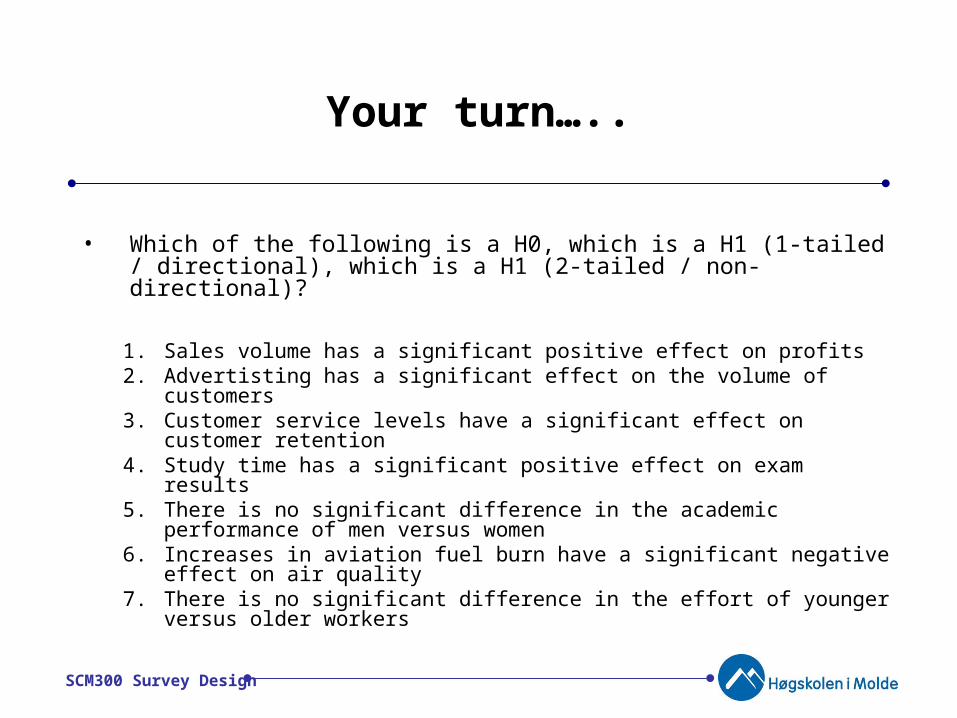
Your turn…..

• Which of the following is a H0, which is a H1 (1-tailed / directional), which is a H1 (2-tailed / non-directional)?

1. Sales volume has a significant positive effect on profits2. Advertisting has a significant effect on the volume of customers3. Customer service levels have a significant effect on customer

retention4. Study time has a significant positive effect on exam results5. There is no significant difference in the academic performance of

men versus women6. Increases in aviation fuel burn have a significant negative effect on

air quality7. There is no significant difference in the effort of younger versus

older workers


Your Survey

You are expected to develop a research question(s) based on theoretical context

Example• Customer-supplier relationships affect the

performance of supply chain networks (Ellinger et al, 1999). This has never been investigated in Norway so this study asks:

Do customer-supplier relationships affect the performance of supply chain networks in Norway?


Your Survey

• The study by Ellinger et al. (1999) and others such as Jammernegg & Kischka (2005) suggest that frequent customer satisfaction surveys affect performance.

• Discussions with industry experts (e.g…..) suggest performance may also be affected by the frequency of meetings with customers and personal visits by senior managers.

• This study will investigate the overall effect of the customer-supplier relationship as well as the effect of individual aspects of the customer-supplier relationship

• What variables are needed…..?


Your Survey

• Variables:– Performance– Customer-supplier relationship

• Frequent customer satisfaction surveys• Frequency of meetings with customers• Personal visit by senior managers

• How might you create the variables using a survey?

• What hypotheses might you use…..?


Statistical Analysis

• The significance of each hypothesis is then tested using statistical analysis

• The objective is to ‘prove’ or ‘disprove’ each hypothesis


What Tests?

Task Data Types of V Test

Relationship between 2 variables

Cross-tabs of frequencies

Nominal Chi-square

Difference between 2 means – paired

Means – whole sample

Ratio or ordinal t-test - paired

Difference between 2 means independent samples

Means – 2 sub-groups

-Ratio or ordinal (means)

-Nominal (2 groups only)

t-test – independent samples


Means – 3+ sub-groups

-Ratio or ordinal (means)

-Nominal (3+ groups)

One-way analysis of variance (ANOVA)


What Tests?

Task Data Types of V Test

Relationship between 3+ variables

Means – cross tabulated

- Ratio or ordinal (means)

- Nominal (2+)

Factorial analysis of variance


Individual measures

Ratio or ordinal (2)

Correlation

Linear relationship between 2 variables

Individual measures

Ratio or ordinal (2)

Linear regression

Linear relationship between 3+ variables

Individual measures

Ratio or ordinal (3+)

Multiple regression

Relationship between large no.s of variables

Individual measures

Ratio or ordinal Factor or cluster analysis


Nature of the Question

The way a question is posed suggests different statistical tests

Inferential statisticsAre there differences in levels of satisfaction between younger

and older students?

Are younger students more satisfied with their course than older students?

Measures of associationIs there a relationship between

age of student and levels of satisfaction?


Inferential Statistics

• Chi-square• One Sample t-test• Paired Samples t-test• Independent Samples t-test• One-Way Analysis of Variance (ANOVA)


Chi-square

• Crosstabs can provide initial analysis but…..– It is difficult to interpret the data– It does not comment on the significance of any

differences

• Chi-square can be used to investigate the significance of the difference between observed and expected values– Used for 2 nominal variables

• e.g. course enrolments & gender


Chi-squareCross-tabulations may suggest a trend

e.g. course enrolments according to gender

Course * Gender Crosstabulation

Count

7 16 23

9 5 14

9 4 13

25 25 50

BSc

MSc

PhD

Course

Total

Female Male

Gender

Total


Chi-square Procedure SPSS

1. Analyse2. Descriptive statistics3. Crosstabs4. Select a variable for rows5. Select a variable for columns6. Statistics7. Tick Chi-square8. Cells9. Tick Expected10. Continue11. OK


Chi-square Output SPSS

• Use Pearson Chi-square• The value is 6.588

– The greater the value, the greater the difference between observed and expected values

• Significance of the difference is 0.037 (i.e. 3.7%)– This means we can be 96.3% confident that the difference is

not down to chance

• We therefore reject the null hypothesis and accept the alternative hypothesis

Chi-Square Tests

6,588a 2 ,037

6,750 2 ,034

5,649 1 ,017

50

Pearson Chi-Square

Likelihood Ratio

Linear-by-LinearAssociation

N of Valid Cases

Value dfAsymp. Sig.

(2-sided)

0 cells (,0%) have expected count less than 5. Theminimum expected count is 6,50.

a.


Probability - remember this…..?

Probability as %

Probability on a 0-1 scale (p)

Confidence level

5 0.05 95%

1 0.01 99%

0.1 0.001 99.9%

i.e. 95% confidence level means we are saying that we believe that there is a 95% chance that what we found is true

(and 5% chance that it is not): written as p<0.05


One Sample t-test

• Compares the mean of a single sample with the population mean– e.g. a University claims that it’s BSc graduates

have an average starting salary that is ’significantly’ higher than the national average


One Sample t-test Procedure SPSS

• Analyse• Compare means• One Sample t-test• Enter test variable

– i.e. graduate salary of the sample

• Enter test value– i.e. national average of 2.5mn NOK

• OK


One Sample t-test Output SPSS

• Sample average of 2.6mn NOK is higher than the national average of 2.5mn NOK (t=1.551)

• But the difference is not significant (p=0.135)• Accept null hypothesis, reject alternative

One-Sample Statistics

23 2615217 356254,11724 74284,12GradSalaryN Mean Std. Deviation

Std. ErrorMean

One-Sample Test

1,551 22 ,135 115217,39 -38838,4 269273,2GradSalaryt df Sig. (2-tailed)

MeanDifference Lower Upper

95% ConfidenceInterval of the

Difference

Test Value = 2500000


Paired & Independent Samples t-tests

• Compares 2 means– i.e. are they statistically different?

• ORDINAL or RATIO variables• Two main situations:

– Compare means of 2 variables for whole sample• Paired samples test e.g. average spend on shoes v food

– Compare means of 1 variable for 2 sub-groups• Independent samples test e.g. average spend on shoes

by men v women


Paired Samples t-test Procedure SPSS

Average spend on shoes v food• Analyse• Compare means• Paired Samples t-test• Select the two variables to be compared• OK


Paired Samples t-test Output SPSS

• Averages can be compared• t = -0.937 (food spend is lower)• But the difference is not significant (p=0.353,

i.e. 35.3%)• Accept null hypothesis, reject alternative

Paired Samples Test

-6,26000 47,22582 6,67874 -19,68143 7,16143 -,937 49 ,353FoodSpend - ShoeSpendPair 1Mean Std. Deviation

Std. ErrorMean Lower Upper


Difference

Paired Differences

t df Sig. (2-tailed)

Paired Samples Statistics

44,4200 50 40,25282 5,69261

50,6800 50 33,77986 4,77719

FoodSpend

ShoeSpend

Pair1

Mean N Std. DeviationStd. Error

Mean


Independent Samples t-test Procedure SPSS

Average spend on shoes by men v women 1. Analyse2. Compare means3. Independent Samples t-test4. Select the test variable

• i.e. shoe spend

5. Select the grouping variable• i.e. gender

6. Define groups for the grouping variable• i.e. 1 for group 1 and 2 for group 2 – this corresponds to 1

for female and 2 for male

7. OK


• Averages can be compared• t = 5.862 (female more than male)• Difference is significant (p=0.000, i.e. 99.9%+)• Reject null hypothesis, accept alternative

Independent Samples t-test Output SPSS

Group Statistics

25 72,2800 29,91310 5,98262

25 29,0800 21,51534 4,30307

GenderFemale

Male

ShoeSpendN Mean Std. Deviation

Std. ErrorMean

Independent Samples Test

2,652 ,110 5,862 48 ,000 43,20000 7,36941 28,38282 58,01718

5,862 43,589 ,000 43,20000 7,36941 28,34399 58,05601

Equal variancesassumed

Equal variancesnot assumed

ShoeSpendF Sig.

Levene's Test forEquality of Variances

t df Sig. (2-tailed)Mean

DifferenceStd. ErrorDifference Lower Upper


Difference

t-test for Equality of Means


• t-test examines differences between 2 means• Analysis of Variance (ANOVA) examines 3+

means– e.g. average spend on shoes by course (BSc, MSc,

PhD)

• Examines whether means for each group vary– Labelled as ’between groups’ in the output

One-Way ANOVA


Average spend on shoes by course

1. Analyse

2. Compare means

3. One-Way Anova

4. Select the DV• i.e. shoe spend

5. Select the factor• i.e. course

6. OK

One-Way ANOVA Procedure SPSS


• F = 3.966 (variance test statistic)• Differences are significant (p=0.026, i.e. 2.6%)• Reject null hypothesis, accept alternative

One-Way ANOVA Output SPSS

ANOVA

ShoeSpend

8073,620 2 4036,810 3,966 ,026

47839,260 47 1017,857

55912,880 49

Between Groups

Within Groups

Total

Sum ofSquares df Mean Square F Sig.


Measures of Association

• Correlation Analysis• Linear Regression Analysis• Multiple Regression Analysis


Correlation Analysis

• Examines relationship between 2 or more ORDINAL or INTERVAL/RATIO variables

• They are ‘CORRELATED’ if they are systematically related– POSITIVELY: as one increases, so does other– NEGATIVELY: as one decreases, so does other– UN-CORRELATED: no relationship


Correlation Analysis

• Correlation is measured by the correlation co-efficient, ‘r’. The co-efficient is:

• Helps to think of correlation in visual terms– e.g. see next slide

Perfect –ve

Moderate –ve

No rel. Moderate +ve

Perfect +ve

-1 -0.7 -0.5 -0.1 0 0.1 0.5 0.7 1

Strong -ve

Weak –ve

Weak +ve

Strong +ve


y

xr close to 1

y

xr close to -1

y

x

y

xboth of these would have r close to 0


Association for Income & Profit

Business Income

(NOKmn)

Profit

(NOKmn)

Business Income

(NOKmn)

Profit

(NOKmn)

1 370 308 14 283 208

2 283 211 15 275 204

3 360 264 16 284 201

4 361 242 17 264 191

5 386 260 18 329 223

6 361 252 19 334 252

7 307 257 20 334 249

8 326 225 21 285 294

9 309 300 22 276 224

10 256 194 23 297 237

11 312 221 24 290 223

12 361 263 25 350 232

13 274 177 26 315 238


Scatter-plot Procedure SPSS

1. Graphs

2. Interactive

3. Scatterplot

4. IV for the x-axis

5. DV for the y-axis

6. OK


Scatter-plot Output SPSS


Correlation Procedure SPSS

1. Analyse

2. Correlate

3. Bivariate

4. Add variables to variables list

5. Tick Pearson’s for interval/ratio data (Spearman’s for ordinal)

6. OK


• r = .617 (moderate-strong positive relationship)• Relationship is significant (p=0.001, i.e. 0.1%)• Reject null hypothesis, accept alternative

Correlation Output SPSS

Correlations

1 .617**

. .001

26 26

.617** 1

.001 .

26 26

Pearson Correlation

Sig. (2-tailed)

N

Pearson Correlation

Sig. (2-tailed)

N

INCOME

PROFIT

INCOME PROFIT

Correlation is significant at the 0.01 level(2-tailed).

**.


Linear Regression Analysis

• Correlation shows strength of relationship but not the causality– Causality indicates the likely impact of IV on DV– e.g. How many pax would visit AMS if more flights

were provided (forecasting)

• Regression calculates equation for ‘best fit line’:y = a + bx

a = a constant representing the point the line crosses the y-axisb = a co-efficient representing the gradient of the slope

y & x = DV & IV


Region Sales (NOKmn) Profits (NOKmn)

North East 1181 38.4

North West 1140 49.3

Yorkshire Humber 740 31.9

East Midlands 1050 39.9

West Midlands 1165 52.1

East of England 1129 32.1

London 1134 65.4

South East 1497 58.9

South West 687 30

Wales 912 27.2

Scotland 808 26.6

Northern Ireland 551 10.3

Annual ticket sales & profits data p/region for HiMolde Airlines


xy scatter plot indicates possible linear relationship (or not)


Best Fit Line

• Perhaps we wish to predict profit for given values of sales– Profit is the dependent variable (y)– Sales the independent variable (x)

• Data seems scattered around a straight line• Then need to find the equation of a ‘best fit’ line:

y = a + bxProfit = ‘a number’ + (‘some other number’ x sales)


Linear Regression Procedure SPSS

1. Analyse

2. Regression

3. Linear

4. Place DV and IV in relevant box

5. OK


Coefficientsa

-9,237 11,080 -,834 ,424

,048 ,011 ,815 4,446 ,001

(Constant)

SalesNOKmn

Model1

B Std. Error

UnstandardizedCoefficients

Beta

StandardizedCoefficients

t Sig.

Dependent Variable: ProfitsNOKmna.

Model Summary

,815a ,664 ,630 9,46114Model1

R R SquareAdjustedR Square

Std. Error ofthe Estimate

Predictors: (Constant), SalesNOKmna.

Linear Regression Output SPSS

Profit = a + b x sales

Extent to which DV can be predicted by the

IV(s) i.e. 66%

Effect of IV on DV is

significant (p=0.001, i.e.

0.1%)


Best Fit Line Procedure SPSS

1. Analyse

2. Regression

3. Curve estimation

4. Place DV and IV in relevant box

5. Tick linear

6. OK


Best Fit Line


Multiple Regression Analysis

• Other factors/IVs may affect DV– i.e. A study may find that:

• ‘Airline choice is dependent on income’

– But airline choice may actually be dependent on age or occupation and income may just be a consequence of those factors

• Multiple regression tries to control for such effects


Region Sales (NOKmn) Customers (mn) Profit (NOKmn)

North East 1181 36 38.4

North West 1140 47 49.3

Yorkshire Humber 740 29 31.9

East Midlands 1050 39 39.9

West Midlands 1165 52 52.1

East of England 1129 31 32.1

London 1134 68 65.4

South East 1497 59 58.9

South West 687 29 30

Wales 912 28 27.2

Scotland 808 24 26.6

Northern Ireland 551 15 10.3

Annual ticket sales, customers & profit data p/region for HiMolde Airlines


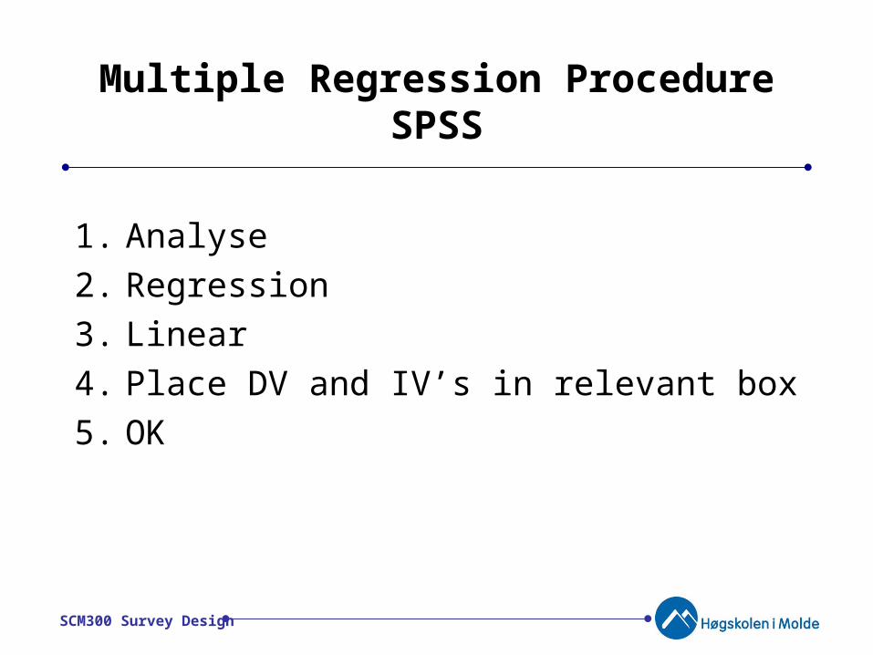
Multiple Regression Procedure SPSS

1. Analyse

2. Regression

3. Linear

4. Place DV and IV’s in relevant box

5. OK


Coefficientsa

-1,745 2,781 -,628 ,546

,005 ,004 ,089 1,215 ,255

,920 ,073 ,919 12,548 ,000

(Constant)

SalesNOKmn

Customersmn

Model1

B Std. Error

UnstandardizedCoefficients

Beta

StandardizedCoefficients

t Sig.

Dependent Variable: ProfitsNOKmna.

Model Summary

,991a ,982 ,978 2,31904Model1

R R SquareAdjustedR Square

Std. Error ofthe Estimate

Predictors: (Constant), Customersmn, SalesNOKmna.

Multiple Regression Output SPSS


Summary

• Variables are defined as a DV or as IV’s– A dependent variable is influenced by changes in the

independent variable(s)

• Hypotheses test specific propositions– They can be null or alternative (one-tailed or two-tailed)

• Statistical tests measure the significance of each hypothesis (and prove or disprove them)

• Inferential statistics measure differences• Measures of association measure relationships


Recommended Reading

• Chapters 4-9 in Gaur, A.S. and Gaur, S.S. (2006). Statistical Methods for Practice and Research: A Guide to Data Analysis Using SPSS. New Delhi: Response Books.


“Thank you for your attention”

Questions.…….

SCM300 Survey Design Lecture 4 Statistical Analysis For use in fall semester 2015 Lecture notes were...

Documents

Transcript of SCM300 Survey Design Lecture 4 Statistical Analysis For use in fall semester 2015 Lecture notes were...