Scilab Manual for Signals and Systems by Dr Dr. R. Anjana ...
54
Scilab Manual for Signals and Systems by Dr Dr. R. Anjana Electrical Engineering Laxmi Institute Of Technology, Sarigam, Gujarat 1 Solutions provided by Dr Dr. R. Anjana Electrical Engineering Laxmi Institute Of Technology, Sarigam, Gujarat February 12, 2022 1 Funded by a grant from the National Mission on Education through ICT, http://spoken-tutorial.org/NMEICT-Intro. This Scilab Manual and Scilab codes written in it can be downloaded from the ”Migrated Labs” section at the website http://scilab.in
Transcript of Scilab Manual for Signals and Systems by Dr Dr. R. Anjana ...

Scilab Manual forSignals and Systemsby Dr Dr. R. AnjanaElectrical Engineering
Laxmi Institute Of Technology, Sarigam,Gujarat1
Solutions provided byDr Dr. R. Anjana
Electrical EngineeringLaxmi Institute Of Technology, Sarigam, Gujarat
February 12, 2022
1Funded by a grant from the National Mission on Education through ICT,http://spoken-tutorial.org/NMEICT-Intro. This Scilab Manual and Scilab codeswritten in it can be downloaded from the ”Migrated Labs” section at the websitehttp://scilab.in

1
Contents
List of Scilab Solutions 4
1 Waveform generation for continuous signals 6
2 Waveform generation for Discrete signals 10
3 Basic Operations on DT signals 14
4 ADDITION AND MULTIPLICATION ON DT SIGNALS 18
5 EVEN and ODD SIGNALS 22
6 Linear and Non-linear Signals 25
7 Energy and Power Signal 29
8 Time Variance and Time Invariance 31
9 DISCRETE CONVOLUTION 34
10 Z- TRANSFORMS AND INVERSE Z - TRANFORM 37
11 Fourier Transform 39
12 Fourier Series 43
13 Causal and Non-Causal 46
14 Sampling Theorem 48
2

15 Sampling rate Conversion 51
3
List of Experiments
Solution 1.01 PROGRAM TO GENERATE COMMON CON-TINUOUS TIME SIGNALS . . . . . . . . . . . . 6
Solution 2.02 PROGRAMTOGENERATE COMMONDISCRETETIME SIGNALS . . . . . . . . . . . . . . . . . . 10
Solution 3.03 TO PERFORM BASIC OPERATIONS ON DTSIGNALS . . . . . . . . . . . . . . . . . . . . . . 14
Solution 4.04 To perform addition and subtraction of the follow-ing two DT signals . . . . . . . . . . . . . . . . . 18
Solution 5.05 EVEN and ODD SIGNALS . . . . . . . . . . . . 22Solution 6.06 To find wheather the system is linear or non linear
for the given signal . . . . . . . . . . . . . . . . . 25Solution 7.7 To find the energy and power of a signal . . . . . 29Solution 8.08 To find wheather the signal is time variant or time
invariant for the signal . . . . . . . . . . . . . . . 31Solution 9.09 To perform discrete convolution for two given se-
quences . . . . . . . . . . . . . . . . . . . . . . . 34Solution 10.10 To find Z Transform and inverse Z Transform for
the given sequence . . . . . . . . . . . . . . . . . 37Solution 11.11 Fourier Transform . . . . . . . . . . . . . . . . . . 39Solution 12.12 Write a program to find the fourier series coeffi-
cients of a signal . . . . . . . . . . . . . . . . . . 43Solution 13.13 To find whether the system is causal or non causal 46Solution 14.14 To find the sampling theoram . . . . . . . . . . . 48Solution 15.15 Sampling Rate Conversion . . . . . . . . . . . . . 51
4
List of Figures
1.1 PROGRAMTOGENERATE COMMONCONTINUOUS TIMESIGNALS . . . . . . . . . . . . . . . . . . . . . . . . . . . . 7
2.1 PROGRAM TO GENERATE COMMON DISCRETE TIMESIGNALS . . . . . . . . . . . . . . . . . . . . . . . . . . . . 11
3.1 TO PERFORM BASIC OPERATIONS ON DT SIGNALS . 15
4.1 To perform addition and subtraction of the following two DTsignals . . . . . . . . . . . . . . . . . . . . . . . . . . . . . . 19
5.1 EVEN and ODD SIGNALS . . . . . . . . . . . . . . . . . . 23
6.1 To find wheather the system is linear or non linear for thegiven signal . . . . . . . . . . . . . . . . . . . . . . . . . . . 26
8.1 To find wheather the signal is time variant or time invariantfor the signal . . . . . . . . . . . . . . . . . . . . . . . . . . 32
9.1 To perform discrete convolution for two given sequences . . . 35
11.1 Fourier Transform . . . . . . . . . . . . . . . . . . . . . . . . 40
12.1 Write a program to find the fourier series coefficients of a signal 44
14.1 To find the sampling theoram . . . . . . . . . . . . . . . . . 49
5

Experiment: 1
Waveform generation forcontinuous signals
Scilab code Solution 1.01 PROGRAMTOGENERATE COMMONCON-TINUOUS TIME SIGNALS
1 // VERSION : S c i l a b : 5 . 4 . 12 // OS : windows 73 // CAPTION: PROGRAM TO GENERATE COMMON CONTINUOUS
TIME SIGNALS4
5 //UNIT IMPULSE SIGNAL6 clc;
7 clear all;
8 close;
9 N=5; //SET LIMIT10 t1= -5:5;
11 x1=[ zeros(1,N),ones (1,1),zeros(1,N)];
12 subplot (2,3,1);
13 plot(t1,x1)
14 xlabel( ’ t ime ’ );15 ylabel( ’ Amplitude ’ );
6

Figure 1.1: PROGRAM TO GENERATE COMMON CONTINUOUS TIMESIGNALS
7

16 title( ’ Unit impu l s e s i g n a l ’ );17
18
19
20 //UNIT STEP SIGNAL21 t2=0:4;
22 x2=ones (1,5);
23 subplot (2,3,2);
24 plot(t2,x2);
25 xlabel( ’ t ime ’ );26 ylabel( ’ ampl i tude ’ );27 title( ’ Unit Step Cont inuous S i g n a l ’ );28
29 title( ’ Unit s t e p s i g n a l ’ );30
31 //EXPONENTIAL SIGNAL32 t3 =0:1:20;
33 x3=exp(-t3);
34 subplot (2,3,3);
35 plot(t3,x3);
36 xlabel( ’ t ime ’ );37 ylabel( ’ Amplitude ’ );38 title( ’ Exponen t i a l s i g n a l ’ );39
40
41
42 //UNIT RAMP SIGNAL43 t4= -0:20;
44 x4=t4;
45 subplot (2,3,4);
46 plot(t4,x4);
47 xlabel( ’ t ime ’ );48 ylabel( ’ Amplitude ’ );49 title( ’ Unit ramp s i g n a l ’ );50
51 //SINUSOIDAL SIGNAL52 t5 =0:0.04:1;
53 x5=sin(2* %pi*t5);
8

54 subplot (2,3,5);
55 plot(t5,x5);
56 title( ’ S i n u s o i d a l S i g n a l ’ )57 xlabel( ’ t ime ’ );58 ylabel( ’ Amplitude ’ );59
60 //RANDOM SIGNAL61 t6= -10:1:20;
62 x6=rand (1,31);
63 subplot (2,3,6);
64 plot(t6,x6);
65 xlabel( ’ t ime ’ );66 ylabel( ’ Amplitude ’ );67 title( ’Random s i g n a l ’ );
9

Experiment: 2
Waveform generation forDiscrete signals
Scilab code Solution 2.02 PROGRAMTOGENERATE COMMONDIS-CRETE TIME SIGNALS
1 // VERSION : S c i l a b : 5 . 4 . 12 // OS : windows 73 // CAPTION: PROGRAM TO GENERATE COMMON DISCRETE TIME
SIGNALS4
5 //UNIT IMPULSE SIGNAL6 clc;
7 clear all;
8 close;
9 N=5; //SET LIMIT10 t1= -5:5;
11 x1=[ zeros(1,N),ones (1,1),zeros(1,N)];
12 subplot (2,4,1);
13 plot2d3(t1,x1)
14 xlabel( ’ t ime ’ );15 ylabel( ’ Amplitude ’ );
10
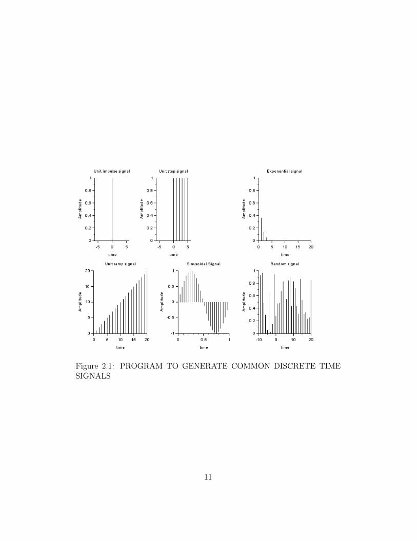
Figure 2.1: PROGRAM TO GENERATE COMMON DISCRETE TIMESIGNALS
11
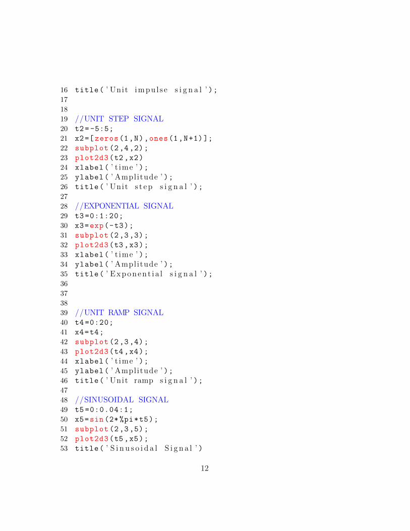
16 title( ’ Unit impu l s e s i g n a l ’ );17
18
19 //UNIT STEP SIGNAL20 t2= -5:5;
21 x2=[ zeros(1,N),ones(1,N+1)];
22 subplot (2,4,2);
23 plot2d3(t2,x2)
24 xlabel( ’ t ime ’ );25 ylabel( ’ Amplitude ’ );26 title( ’ Unit s t e p s i g n a l ’ );27
28 //EXPONENTIAL SIGNAL29 t3 =0:1:20;
30 x3=exp(-t3);
31 subplot (2,3,3);
32 plot2d3(t3,x3);
33 xlabel( ’ t ime ’ );34 ylabel( ’ Amplitude ’ );35 title( ’ Exponen t i a l s i g n a l ’ );36
37
38
39 //UNIT RAMP SIGNAL40 t4 =0:20;
41 x4=t4;
42 subplot (2,3,4);
43 plot2d3(t4,x4);
44 xlabel( ’ t ime ’ );45 ylabel( ’ Amplitude ’ );46 title( ’ Unit ramp s i g n a l ’ );47
48 //SINUSOIDAL SIGNAL49 t5 =0:0.04:1;
50 x5=sin(2* %pi*t5);
51 subplot (2,3,5);
52 plot2d3(t5,x5);
53 title( ’ S i n u s o i d a l S i g n a l ’ )
12

54 xlabel( ’ t ime ’ );55 ylabel( ’ Amplitude ’ );56
57 //RANDOM SIGNAL58 t6= -10:1:20;
59 x6=rand (1,31);
60 subplot (2,3,6);
61 plot2d3(t6,x6);
62 xlabel( ’ t ime ’ );63 ylabel( ’ Amplitude ’ );64 title( ’Random s i g n a l ’ );
13
Experiment: 3
Basic Operations on DT signals
Scilab code Solution 3.03 TO PERFORM BASIC OPERATIONS ONDT SIGNALS
1 // VERSION : S c i l a b : 5 . 4 . 12 // OS : windows 73
4 //CAPTION:TO PERFORM BASIC OPERATIONS ON D.T SIGNALS5
6 clc;
7 clear all;
8 close;
9
10 // amp l i f i c a t i o n11 x=input( ’ Enter i nput s equence x : ’ );12 a=input( ’ Enter amp l i f i c a t i o n f a c t o r a : ’ );13 b=input( ’ Enter a t t e nu a t i o n f a c t o r b : ’ );14 c=input( ’ Enter ampl i tude r e v e r s a l f a c t o r c : ’ );15 y1=a*x;
16 y2=b*x;
17 y3=c*x;
18 n=length(x);
14

Figure 3.1: TO PERFORM BASIC OPERATIONS ON DT SIGNALS
15
19
20 // Input s i g n a l p l o t21 subplot (2,3,1);
22 plot2d3 (0:n-1,x);
23 xlabel( ’ t ime ’ );24 ylabel( ’ ampl i tude ’ );25 title( ’ Input s i g n a l ’ );26
27 // Amp l i f i c a t i o n28 subplot (2,3,2);
29 plot2d3 (0:n-1,y1);
30 xlabel( ’ t ime ’ );31 ylabel( ’ Amplitude ’ );32 title( ’ Amp l i f i ed s i g n a l ’ );33
34 // a t t e nu a t i o n35 subplot (2,3,3);
36 plot2d3 (0:n-1,y2);
37 xlabel( ’ t ime ’ );38 ylabel( ’ Amplitude ’ );39 title( ’ Attenuated s i g n a l ’ );40
41 // Amplitude Rev e r a s l42 subplot (2,3,4);
43 plot2d3 (0:n-1,y3);
44 xlabel( ’ t ime ’ );45 ylabel( ’ Amplitude ’ );46 title( ’ Amplitude r e v e r s a l s i g n a l ’ );47
48 // f o l d i n g and S h i f t i n g49
50 n0=input( ’ Enter the +ve s h i f t : ’ );51 n1=input( ’ Enter the −ve s h i f t : ’ );52 l=length(x);
53 i=n0:l+n0 -1;
54 j=n1:l+n1 -1;
55 subplot (2,3,5);
56 plot2d3(i,x);
16

57 xlabel( ’ t ime ’ );58 ylabel( ’ Amplitude ’ );59 title( ’ P o s i t i v e s h i f t e d s i g n a l ’ );60 subplot (2,3,6);
61 plot2d3(j,x);
62 xlabel( ’ t ime ’ );63 ylabel( ’ Amnplitude ’ );64 title( ’ Nega t i v e s h i f t e d s i g n a l ’ );65
66
67 // ∗∗∗∗∗∗∗∗∗∗∗∗∗∗∗∗∗∗∗∗∗∗∗∗∗∗//68 //INPUT : In Conso l e Window69 // ∗∗∗∗∗∗∗∗∗∗∗∗∗∗∗∗∗∗∗∗∗∗∗∗//70
71 // Enter the Input Sequence x ( n ) =[1 2 3 4 5 ]72 // Enter the amp l i f i c a t i o n f a c t o r a = 0 . 373 // Enter the a t t e n u a t i o n f a c t o r b = 0 . 574 // Enter the ampl i tude r e v e r s a l f a c t o r c = −375 // Enter the p o s i t i v e s h i f t : 276 // Enter the n e g a t i v e s h i f t : −577
78 //OUTPUT: In Graphic Windows
17

Experiment: 4
ADDITION ANDMULTIPLICATION ON DTSIGNALS
Scilab code Solution 4.04 To perform addition and subtraction of the fol-lowing two DT signals
1 // VERSION : S c i l a b : 5 . 4 . 12 // OS : windows 73
4 //CAPTION: To per fo rm add i t i o n and s u b t r a c t i o n o fthe f o l l o w i n g two DT s i g n a l s
5 //Xa( t ) = 1 ; 0<t<16 // 2 ; 1<t <2;7 // 1 ; 2<t<38
9 // &10 // Xb( t ) = t ; 0<t<111 // 1 ; 1<t <2;12 // 3− t ; 2<t<313
18
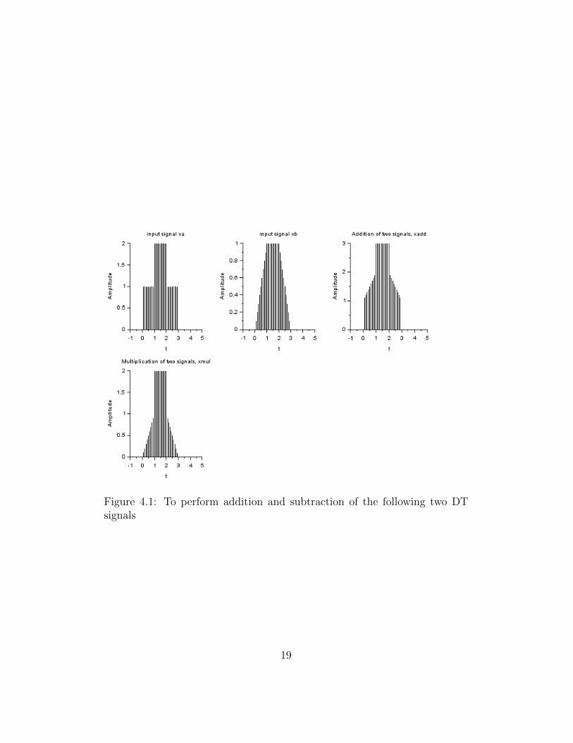
Figure 4.1: To perform addition and subtraction of the following two DTsignals
19

14 //////∗∗∗∗∗∗∗∗∗∗∗∗∗∗∗∗∗∗∗∗∗∗∗∗∗∗∗∗∗∗∗////////////////////////
15
16 clc;
17 clear all;
18 close
19 t = -1:0.1:5;
20 x1 = 1;
21 x2 = 2;
22 x3 = 3-t;
23
24 xa = x1.*(t>0 & t<1) + x2.*(t>=1 & t<=2) + x1.*(t>2
& t<3);
25 xb = t.*(t>0 &t<1) + x1*(t>=1 &t<=2)+x3.*(t>2 &t<3);
26
27 xadd = xa +xb;
28 xmul = xa.*xb;
29 subplot (2,3,1);
30 plot2d3(t,xa) // P l o t s i nput s i g n a l xa31 xlabel( ’ t ’ );32 ylabel( ’ Amplitude ’ );33 title( ’ i npu t s i g n a l xa ’ );34 subplot (2,3,2);
35 plot2d3(t,xb) // P l o t s i nput s i g n a l xb36 xlabel( ’ t ’ );37 ylabel( ’ Amplitude ’ );38 title( ’ i npu t s i g n a l xb ’ );39 subplot (2,3,3);
40 plot2d3(t,xadd) // P l o t s a d d i t i o n o f s i g n a l xa andxb
41 xlabel( ’ t ’ );42 ylabel( ’ Amplitude ’ );43 title( ’ Add i t i on o f two s i g n a l s , xadd ’ );44 subplot (2,3,4);
45 plot2d3(t,xmul) // P l o t s Mu l t i p l i c a t i o n o f s i g n a l xaand xb
46 xlabel( ’ t ’ );
20

47 ylabel( ’ Amplitude ’ );48 title( ’ M u l t i p l i c a t i o n o f two s i g n a l s , xmul ’ );49
50 // // Output : In Graphic Window
21

Experiment: 5
EVEN and ODD SIGNALS
Scilab code Solution 5.05 EVEN and ODD SIGNALS
1 // VERSION : S c i l a b : 5 . 4 . 12 // OS : windows 73
4 //CAPTION: EVEN and ODD SIGNALS f o r x ( t )=s i n t ( t )+co s( t )
5
6 clc;
7 close;
8 clear all;
9 t=0:.005:4* %pi;
10 x=sin(t)+cos(t); // Given s i g n a l : x ( t )=s i n t ( t )+co s ( t)
11 subplot (2,2,1)
12 plot(t,x)
13 xlabel( ’ t ’ );14 ylabel( ’ ampl i tude ’ )15 title( ’ i npu t s i g n a l ’ )16 y=sin(-t)+cos(-t) // Put t = −t i n x ( t )17 subplot (2,2,2)
22

Figure 5.1: EVEN and ODD SIGNALS
23

18 plot(t,y)
19 xlabel( ’ t ’ );20 ylabel( ’ ampl i tude ’ )21 title( ’ x(− t ) ’ )22 z=x+y
23 subplot (2,2,3)
24 plot(t,z/2) // to p l o t even s i g n a l25 xlabel( ’ t ’ );26 ylabel( ’ ampl i tude ’ )27 title( ’ even pa r t o f the s i g n a l ’ )28 p=x-y
29 subplot (2,2,4)
30 plot(t,p/2) // to p l o t odds s i g n a l31 xlabel( ’ t ’ );32 ylabel( ’ ampl i tude ’ );33 title( ’ odd pa r t o f the s i g n a l ’ );34
35 //Output : In g r aph i c window
24

Experiment: 6
Linear and Non-linear Signals
Scilab code Solution 6.06 To find wheather the system is linear or nonlinear for the given signal
1 // VERSION : S c i l a b : 5 . 4 . 12 // OS : windows 73
4 //CAPTION: To f i n d wheather the system i s l i n e a r ornon l i n e a r f o r the g i v en s i g n a l y ( n ) =[x ( n ) ]ˆ2+B;
5
6 clc;
7 clear all;
8 close;
9
10 // P r o p e r t i e s o f DT Systems ( L i n e a r i t y )11 //y ( n ) =[x ( n ) ]ˆ2+B;12
13 x1=input( ’ Enter f i r s t i nput s equence : ’ );14 n=length(x1);
15 x2=input( ’ Enter second input s equence : ’ );16 a=input( ’ Enter s c a l i n g c on s t an t ( a ) : ’ );17 b=input( ’ Enter s c a l i n g c on s t an t ( b ) : ’ );
25
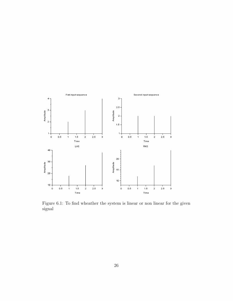
Figure 6.1: To find wheather the system is linear or non linear for the givensignal
26

18 B=input( ’ Enter s c a l i n g c on s t an t (B) : ’ );19
20 y1=x1.^2+B;
21 y2=x2.^2+B;
22 rhs=a*y1+b*y2;
23 x3=a*x1+b*x2;
24 lhs=x3.^2+B;
25
26 subplot (2,2,1);
27 plot2d3 (0:n-1,x1);
28 xlabel( ’ Time ’ );29 ylabel( ’ Amplitude ’ );30 title( ’ F i r s t i nput s equence ’ );31 subplot (2,2,2);
32 plot2d3 (0:n-1,x2);
33 xlabel( ’ Time ’ );34 ylabel( ’ Amplitude ’ );35 title( ’ Second input s equence ’ );36 subplot (2,2,3);
37 plot2d3 (0:n-1,lhs);
38 xlabel( ’ Time ’ );39 ylabel( ’ Amplitude ’ );40 title( ’LHS ’ );41 subplot (2,2,4);
42 plot2d3 (0:n-1,rhs);
43 xlabel( ’ Time ’ );44 ylabel( ’ Amplitude ’ );45 title( ’RHS ’ );46
47 if(lhs==rhs)
48 disp( ’ system i s l i n e a r ’ );49 else
50 disp( ’ system i s non− l i n e a r ’ );51
52 end;
53
54
55 // // Input Data
27

56
57 // Enter f i r s t i nput s equence : [ 1 2 3 4 ]58 // Enter second input s equence : [ 2 2 2 2 ]59 // Enter s c a l i n g c on s t an t ( a ) : 160 // Enter s c a l i n g c on s t an t ( b ) : 161 // Enter s c a l i n g c on s t an t (B) : 262
63 // / Output : system i s non− l i n e a r64 // See g r aph i c window
28

Experiment: 7
Energy and Power Signal
Scilab code Solution 7.7 To find the energy and power of a signal
1 // VERSION : S c i l a b : 5 . 4 . 12 // OS : windows 73
4 //CAPTION: To f i n d the ene rgy and power o f a s i g n a l5
6
7 //To f i n d ene rgy o f a s i g n a l8 clc;
9 clear all;
10 close;
11 E =0;
12 for n =0:50
13 x ( n +1) =( 0.5) ^ n ;
14 end
15 for n =0:100
16 E = E + x (n +1) ^2;
17 end
18 if E < %inf then
19 disp (E , ’ The Energy o f the g i v en s i g n a l i s E = ’ );
20 else
29

21 disp ( ’ The g i v en s i g n a l i s ene rgy s i g n a l i s not anEnergy S i g n a l ’ ) ;
22 end
23
24 // /// To f i n d power o f the S i g n a l25 T=10; // Tota l e v a l u a t i o n t ime26 Ts =0.001; // Sampl ing t ime => ; 1000 sample s per
second27 Fs=1/Ts; // Sampl ing p e r i o d28 t=[0:Ts:T]; // d e f i n e s imu l a t i o n t ime29 x=cos(2*%pi *100*t)+cos (2*%pi *200*t)+sin(2* %pi *300*t)
;
30 power = (norm(x)^2)/length(x);
31 disp(power , ’ The power o f the g i v en s i g n a l i s P = ’ )32
33
34 // output35 //The Energy o f the g i v en s i g n a l i s E =51.33333336
37 // The power o f the g i v en s i g n a l i s P = 1 . 50025
30

Experiment: 8
Time Variance and TimeInvariance
Scilab code Solution 8.08 To find wheather the signal is time variant ortime invariant for the signal
1 // VERSION : S c i l a b : 5 . 4 . 12 // OS : windows 73
4 //CAPTION: To f i n d wheather the s i g n a l i s t imev a r i a n t or t ime i n v a r i a n t f o r the s i g n a l y ( n )=n ∗ [x ( n ) ] ;
5 clc;
6 clear all;
7 close ;
8 x1=input( ’ Enter i nput s equence x1 : ’ );9 n1=length(x1);
10 for n=1:n1
11 y1(n1)=n.*x1(n);
12 end;
13 n0=input( ’ Enter s h i f t : ’ );14 x2=[ zeros(1,n0),x1];
31
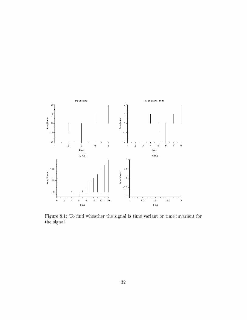
Figure 8.1: To find wheather the signal is time variant or time invariant forthe signal
32

15 for n2=1:n1+n0
16 y2(n2)=n2.*x2(n2);
17 end;
18 y3=[ zeros(1,n0)],y1;
19 if(y2==y3)
20 disp( ’ system i s t ime i n v a r i a n t ’ );21 else
22 disp( ’ system i s t ime v a r i a n t ’ );23 end;
24 subplot (2,2,1);
25 plot2d3(x1);
26 xlabel( ’ t ime ’ );27 ylabel( ’ Amplitude ’ );28 title( ’ Input s i g n a l ’ );29 subplot (2,2,2);
30 plot2d3(x2);
31 xlabel( ’ t ime ’ );32 ylabel( ’ Amplitude ’ );33 title( ’ S i g n a l a f t e r s h i f t ’ );34 subplot (2,2,3);
35 plot2d3(y2);
36 xlabel( ’ t ime ’ );37 ylabel( ’ Amplitude ’ );38 title( ’L .H. S ’ );39 subplot (2,2,4);
40 plot2d3(y3);
41 xlabel( ’ t ime ’ );42 ylabel( ’ Amplitude ’ );43 title( ’R .H. S ’ );44
45
46 // // Sample Input47 // / Enter i nput s equence x1 : [ 1 −1 −2 1 2 ]48 // Enter s h i f t : 349
50 // Output51 // system i s t ime v a r i a n t
33

Experiment: 9
DISCRETE CONVOLUTION
Scilab code Solution 9.09 To perform discrete convolution for two givensequences
1 // VERSION : S c i l a b : 5 . 4 . 12 // OS : windows 73
4 //CAPTION: To per fo rm d i s c r e t e c o nv o l u t i o n f o r twog i v en s e qu en c e s
5
6 clc;
7 clear all;
8 close ;
9 a=input( ’ Enter the s t a r t i n g po i n t o f x [ n]= ’ );10 b=input( ’ Enter the s t a r t i n g po i n t o f h [ n]= ’ );11 x=input( ’ Enter the co− e f f i c i e n t s o f x [ n]= ’ );12 h=input( ’ Enter the co− e f f i c i e n t s o f h [ n]= ’ );13 y=conv(x,h);
14 subplot (3,1,1);
15 p=a:(a+length(x) -1);
16 plot2d3(p,x);
17 xlabel( ’ Time ’ );
34

Figure 9.1: To perform discrete convolution for two given sequences
35
18 ylabel( ’ Amplitude ’ );19 title( ’ INPUT x (n ) ’ );20 subplot (3,1,2);
21 q=b:(b+length(h) -1);
22 plot2d3(q,h);
23 xlabel( ’ Time ’ );24 ylabel( ’ Amplitude ’ );25 title( ’ IMPULSE RESPONSE h ( n ) ’ );26 subplot (3,1,3);
27 n=a+b:length(y)+a+b-1;
28 plot2d3(n,y);
29
30 disp(y)
31 xlabel( ’ Time ’ );32 ylabel( ’ Amplitude ’ );33 title( ’LINEAR CONVOLUTION ’ );34
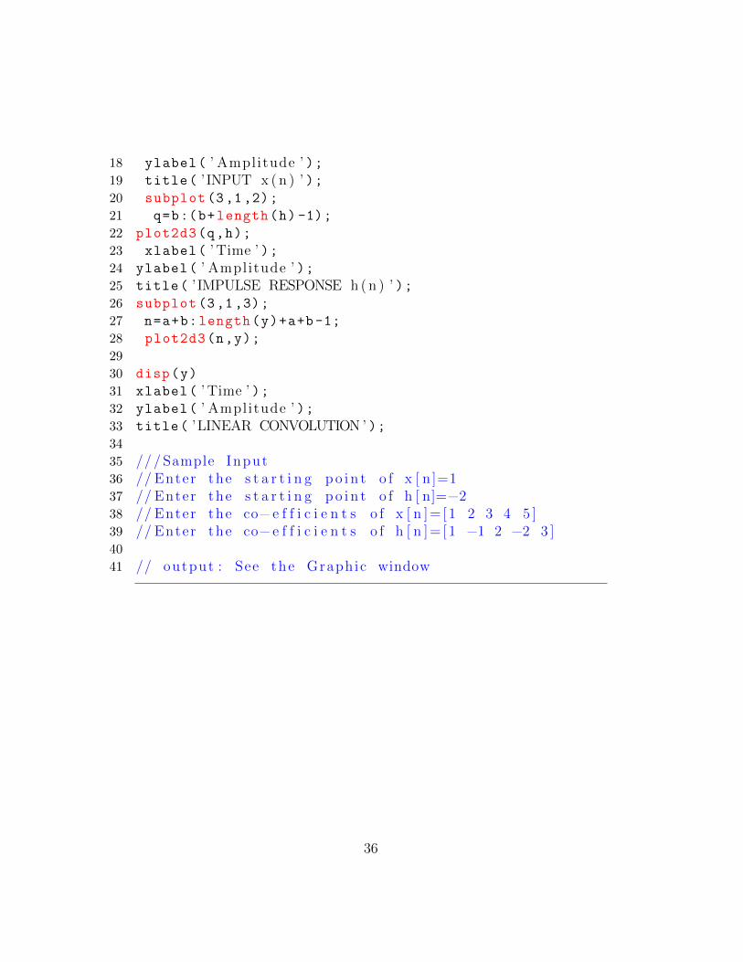
35 // /Sample Input36 // Enter the s t a r t i n g po i n t o f x [ n ]=137 // Enter the s t a r t i n g po i n t o f h [ n]=−238 // Enter the co− e f f i c i e n t s o f x [ n ]= [1 2 3 4 5 ]39 // Enter the co− e f f i c i e n t s o f h [ n ]= [1 −1 2 −2 3 ]40
41 // output : See the Graphic window
36

Experiment: 10
Z- TRANSFORMS ANDINVERSE Z - TRANFORM
Scilab code Solution 10.10 To find Z Transform and inverse Z Transformfor the given sequence
1
2 // VERSION : S c i l a b : 5 . 4 . 13 // OS : windows 74
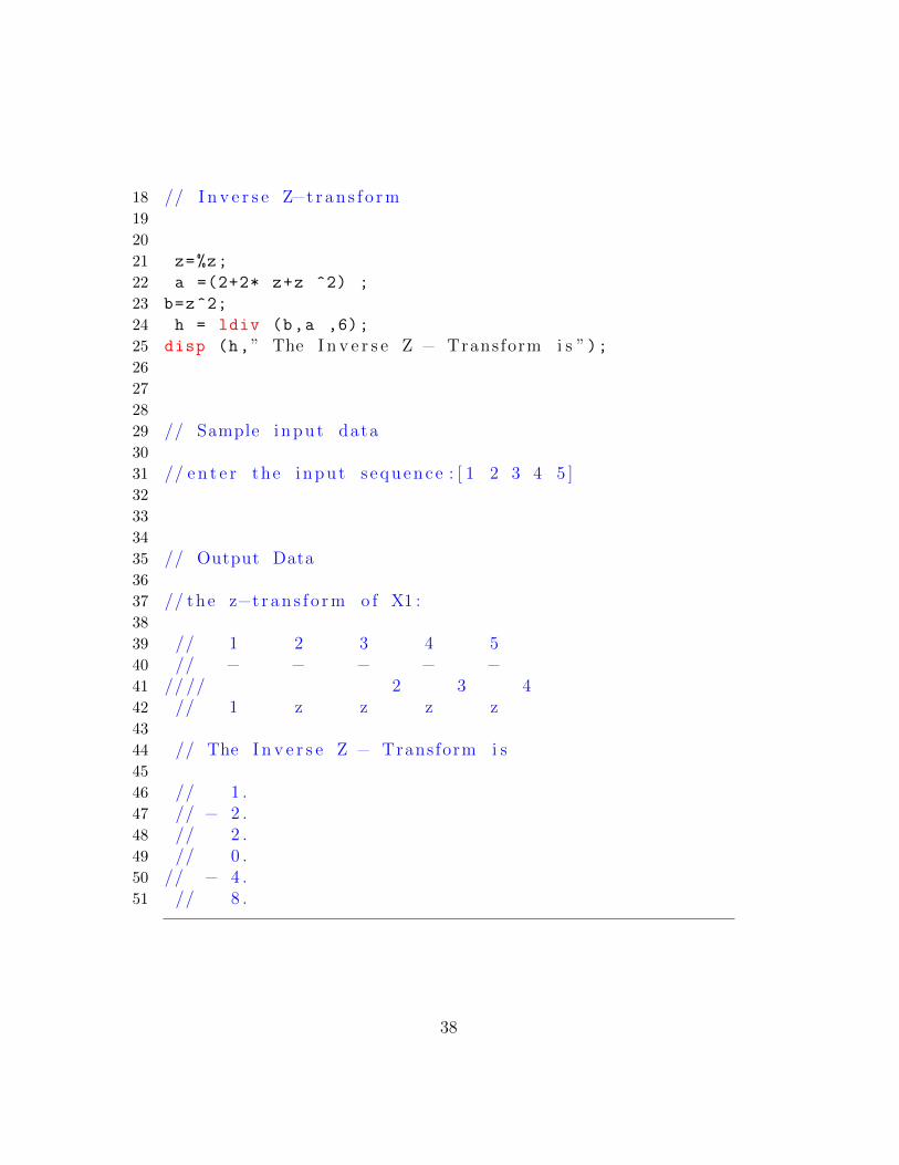
5 //CAPTION: To f i n d Z−Transform and i n v e r s e Z−Transform f o r the g i v en s equence
6
7 // Z t r an s f o rm o f g i v en s equence8 clear all;
9 clc ;
10 close ;
11 z = poly (0 , ’ z ’ , ’ r ’ );12 x1 = input( ’ e n t e r the input s equence : ’ );13 n1 = 0: length ( x1 ) -1;
14 X1 = x1 .*[(1/ z ) .^n1];
15 disp(X1, ’ the z−t r an s f o rm o f X1 : ’ )16
17
37
18 // I n v e r s e Z−t r an s f o rm19
20
21 z=%z;
22 a =(2+2* z+z ^2) ;
23 b=z^2;
24 h = ldiv (b,a ,6);
25 disp (h,” The I n v e r s e Z − Transform i s ”);26
27
28
29 // Sample input data30
31 // e n t e r the input s equence : [ 1 2 3 4 5 ]32
33
34
35 // Output Data36
37 // the z−t r an s f o rm o f X1 :38
39 // 1 2 3 4 540 // − − − − −41 // // 2 3 442 // 1 z z z z43
44 // The I n v e r s e Z − Transform i s45
46 // 1 .47 // − 2 .48 // 2 .49 // 0 .50 // − 4 .51 // 8 .
38

Experiment: 11
Fourier Transform
Scilab code Solution 11.11 Fourier Transform
1 // VERSION : S c i l a b : 5 . 4 . 12 // OS : windows 73
4 //CAPTION:A symmet r i c a l r e c t a n g u l a r pu l s e i s g i v enby R(n ) = 1 ; −N<n<N = 0 ; o t h e rw i s e ;
5 // Determine The DTFT f o r N = {5 , 1 5 , 2 5 , 1 0 0} . S c a l ethe DTFT so tha t x ( 0 ) = 1 , a l s o p l o t theno rma l i z ed DTFT over − to .
6
7
8 clc;
9 clear all;
10 close
11 N=input( ’ Enter The Value Of N1 = ’ );12 n=-N:1:N;
13 x=ones(1,length(n));
14 w=(-%pi:(%pi /100):%pi);
15 z=x*exp(-%i*n’*w);
16 subplot (2,2,1);
39
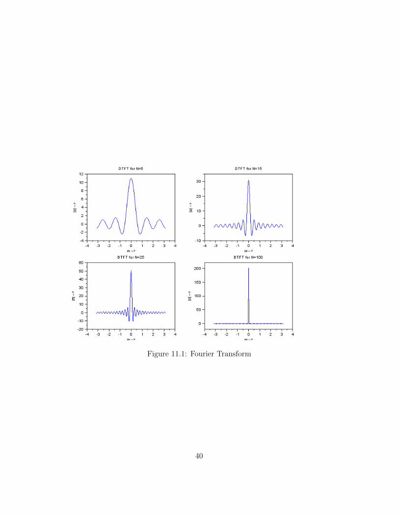
Figure 11.1: Fourier Transform
40
17 plot(w,z);
18 xlabel( ’w −−> ’ );19 ylabel( ’ | z | −−> ’ );20 title( ’DTFT f o r N=5 ’ );21
22 N=input( ’ Enter The Value Of N2 = ’ );23 n=-N:1:N;
24 x=ones(1,length(n));
25 w=(-%pi:(%pi /100):%pi);
26 z=x*exp(-%i*n’*w);
27 subplot (2,2,2);
28 plot(w,z);
29 xlabel( ’w −−> ’ );30 ylabel( ’ | z | −−> ’ );31 title( ’DTFT f o r N=15 ’ );32
33 N=input( ’ Enter The Value Of N3 = ’ );34 n=-N:1:N;
35 x=ones(1,length(n));
36 w=(-%pi:(%pi /100):%pi);
37 z=x*exp(-%i*n’*w);
38 subplot (2,2,3);
39 plot(w,z);
40 xlabel( ’w −−> ’ );41 ylabel( ’ | z | −−> ’ );42 title( ’DTFT f o r N=25 ’ );43
44 N=input( ’ Enter The Value Of N4 = ’ );45 n=-N:1:N;
46 x=ones(1,length(n));
47 w=(-%pi:(%pi /100):%pi);
48 z=x*exp(-%i*n’*w);
49 subplot (2,2,4);
50 plot(w,z);
51 xlabel( ’w −−> ’ );52 ylabel( ’ | z | −−> ’ );53 title( ’DTFT f o r N=100 ’ );54
41
55 // //////////////////////56 // / SAMPLE INPUTS//////57
58 // Enter The Value Of N1 = 559 // Enter The Value Of N2 = 1560 // Enter The Value Of N3 = 2561 // Enter The Value Of N4 = 100
42

Experiment: 12
Fourier Series
Scilab code Solution 12.12 Write a program to find the fourier series co-efficients of a signal
1
2 // VERSION : S c i l a b : 5 . 4 . 13 // OS : windows 74
5 //CAPTION: Write a program to f i n d the f o u r i e rs e r i e s c o e f f i c i e n t s o f a s i g n a l .
6
7 fig_size = [232 84 774 624];
8 x = [0.1 0.9 0.1]; // % 1 pe r i o d o f x ( t )9 x = [x x x x]; //% 4 p e r i o d s o f x ( t )10 tx = [-2 -1 0 0 1 2 2 3 4 4 5 6]; //% time p o i n t s
f o r x ( t )11 subplot (2,2,1)
12 plot(tx,x)
13 xlabel( ’ Time ( s ) ’ )14 ylabel( ’ Amplitude ’ ) ,...15 title( ’ P e r i o d i c S i g n a l x ( t ) ’ )16
43
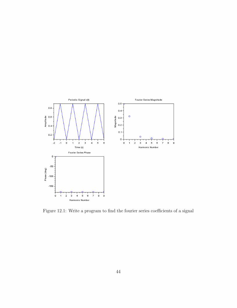
Figure 12.1: Write a program to find the fourier series coefficients of a signal
44

17 a0 = 0.5; // DC component o f Fou r i e r S e r i e s18 ph0 = 0;
19 n = [1 3 5 7 9]; // Values o f n to be eva l u a t ed20 an = -3.2 ./ (%pi * n).^2; //% Fou r i e r S e r i e s
c o e f f i c i e n t s21 mag_an = abs(an);
22 ph_an = -180 * ones(1,length(n));
23 n = [0 n];
24 mag_an = [a0 mag_an ]; // % In c l u d i n g a0 with a n25 ph_an = [ph0 ph_an];
26
27 // P l o t t i n g f o u r i e r s e r i e s magnitude28 subplot (2,2,2)
29 plot(n,mag_an , ’ o ’ );30 xlabel( ’ Harmonic Number ’ );31 ylabel( ’ Magnitude ’ );32 title( ’ F ou r i e r S e r i e s Magnitude ’ )33
34 // P l o t t i n g f o u r i e r s e r i e s phase35 subplot (2,2,3)
36 plot(n,ph_an , ’ o ’ )37 xlabel( ’ Harmonic Number ’ )38 ylabel( ’ Phase ( deg ) ’ )39 title( ’ F ou r i e r S e r i e s Phase ’ ),
45

Experiment: 13
Causal and Non-Causal
Scilab code Solution 13.13 To find whether the system is causal or noncausal
1
2 // VERSION : S c i l a b : 5 . 4 . 13 // OS : windows 74
5 //CAPTION: To f i n d whether the system i s c a u s a l ornon−c a u s a l
6
7 clc;
8 clear all;
9 close;
10 // %Prope r t i e s o f DT Systems ( Cau s a l i t y )11 //%y( n )=x(−n ) ;12
13 x1=input( ’ Enter i nput s equence x1 : ’ );14 n1=input( ’ Enter upper l i m i t n1 : ’ );15 n2=input( ’ Enter l owe r l i m i t n2 : ’ );16 flag =0;
17 for n=n1:n2
18 arg=-n;
19 if arg >n;
46
20 flag =1;
21 end;
22 end;
23 if(flag ==1)
24 disp( ’ system i s c a u s a l ’ );25 else
26 disp( ’ system i s non−c a u s a l ’ );27 end
28
29 // / Sample i npu t s30 // Enter i nput s equence x1 : [ 1 2 −1 3 −4 5 −5]31 // Enter upper l i m i t n1 : 232 // Enter l owe r l i m i t n2 :−233
34 // output :35 // system i s non−c a u s a l
47
Experiment: 14
Sampling Theorem
Scilab code Solution 14.14 To find the sampling theoram
1
2 // VERSION : S c i l a b : 5 . 4 . 13 // OS : windows 74
5 //CAPTION: To f i n d the sampl ing theoram6
7 clc;
8 T=0.04;
9 t=0:0.0005:0.02;
10 f = 1/T;
11 n1 =0:40;
12 size(n1)
13 xa_t=sin(2* %pi*2*t/T);
14 subplot (2,2,1);
15 plot2d3 (200*t,xa_t);
16 title( ’ V e r i f i c a t i o n o f sampl ing theorem ’ );17 title( ’ Cont inuous s i g n a l ’ );18 xlabel( ’ t ’ );19 ylabel( ’ x ( t ) ’ );
48

Figure 14.1: To find the sampling theoram
49
20
21 // g r e a t e r than nyqu i s t r a t e22 ts1 =0.002; //>n iq r a t e23 n=0:20;
24 x_ts1 =2* sin(2*%pi*n*ts1/T);
25 subplot (2,2,2);
26 plot2d3(n,x_ts1);
27 title( ’ g r e a t e r than Nq ’ );28 xlabel( ’ n ’ );29 ylabel( ’ x ( n ) ’ );30
31 // Equal to nyqu i s t r a t e32
33 ts2 =0.01; // n iq r a t e34 n=0:4;
35 x_ts2 =2* sin(2*%pi*n*ts2/T);
36 subplot (2,2,3);
37 plot2d3(n,x_ts2);
38 title( ’ Equal to Nq ’ );39 xlabel( ’ n ’ );40 ylabel( ’ x ( n ) ’ );41
42 // l e s s than nyqu i s t r a t e43 ts3 =0.1; //<n iq r a t e44 n=0:10;
45 x_ts3 =2* sin(2*%pi*n*ts3/T);
46 subplot (2,2,4);
47 plot2d3(n,x_ts3);
48 title( ’ l e s s than Nq ’ );49 xlabel( ’ n ’ );50 ylabel( ’ x ( n ) ’ );
50
Experiment: 15
Sampling rate Conversion
Scilab code Solution 15.15 Sampling Rate Conversion
1 // VERSION : S c i l a b : 5 . 4 . 12 // OS : windows 73
4 //CAPTION: Sampl ing Rate Conver s i on5
6 //Down Sampl ing ( or Dec imat ion ) :7
8 xn = input( ’ Enter the number o f sample s xn : ’ );[1 2
3 4 5 6 8 ]
9 N=length(xn);
10 n=0:1:N-1;
11 D=3;
12 xDn=xn(1:D:N);
13 n1=1:1:N/D;
14 // f i g u r e ;15 disp(xDn , ’ the downsampling ( or ) Dec imat ion f o r D = 3
i s :−−−−−> ’ )16
17 //Up Sampl ing ( or I n t e r p o l a t i o n )18 yn = input( ’ Enter the number o f sample s yn : ’ )// / [ 1
−2 3 4 8 9 10 4 4 ]
51
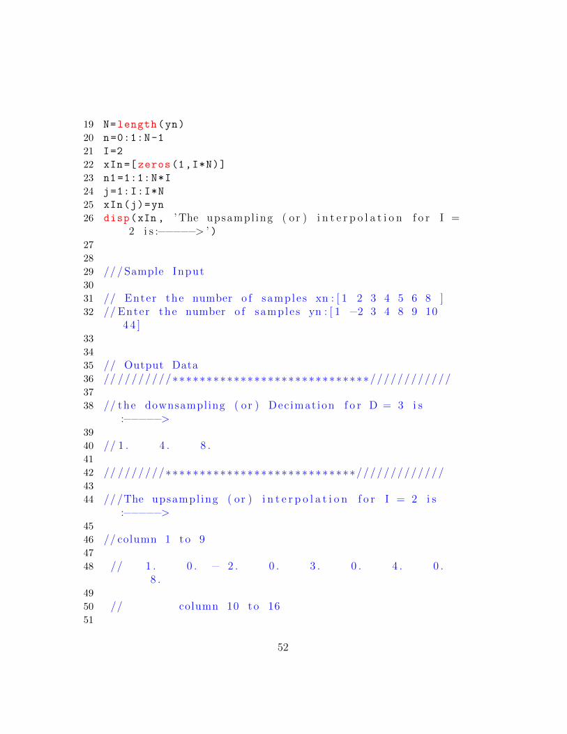
19 N=length(yn)
20 n=0:1:N-1
21 I=2
22 xIn=[zeros(1,I*N)]
23 n1=1:1:N*I
24 j=1:I:I*N
25 xIn(j)=yn
26 disp(xIn , ’ The upsampl ing ( or ) i n t e r p o l a t i o n f o r I =2 i s :−−−−−> ’ )
27
28
29 // /Sample Input30
31 // Enter the number o f sample s xn : [ 1 2 3 4 5 6 8 ]32 // Enter the number o f sample s yn : [ 1 −2 3 4 8 9 10
4 4 ]33
34
35 // Output Data36 // ////////∗∗∗∗∗∗∗∗∗∗∗∗∗∗∗∗∗∗∗∗∗∗∗∗∗∗∗∗∗////////////37
38 // the downsampling ( or ) Dec imat ion f o r D = 3 i s:−−−−−>
39
40 // 1 . 4 . 8 .41
42 // ///////∗∗∗∗∗∗∗∗∗∗∗∗∗∗∗∗∗∗∗∗∗∗∗∗∗∗∗∗/////////////43
44 // /The upsampl ing ( or ) i n t e r p o l a t i o n f o r I = 2 i s:−−−−−>
45
46 // column 1 to 947
48 // 1 . 0 . − 2 . 0 . 3 . 0 . 4 . 0 .8 .
49
50 // column 10 to 1651
52

52 // 0 . 9 . 0 . 1 0 . 0 . 4 4 . 0 .
53