Scikit-plot Documentation

Scikit-plot DocumentationRelease

Reiichiro S. Nakano

Sep 17, 2017

Contents

1 First steps with Scikit-plot 11.1 Installation . . . . . . . . . . . . . . . . . . . . . . . . . . . . . . . . . . . . . . . . . . . . . . . . 11.2 Your First Plot . . . . . . . . . . . . . . . . . . . . . . . . . . . . . . . . . . . . . . . . . . . . . . 11.3 The Functions API . . . . . . . . . . . . . . . . . . . . . . . . . . . . . . . . . . . . . . . . . . . . 31.4 More Plots . . . . . . . . . . . . . . . . . . . . . . . . . . . . . . . . . . . . . . . . . . . . . . . . 5

2 Factory API Reference 72.1 Classifier Plots . . . . . . . . . . . . . . . . . . . . . . . . . . . . . . . . . . . . . . . . . . . . . . 72.2 Clustering Plots . . . . . . . . . . . . . . . . . . . . . . . . . . . . . . . . . . . . . . . . . . . . . 19

3 Functions API Reference 23

4 Indices and tables 39

Python Module Index 41

i

CHAPTER 1

First steps with Scikit-plot

Eager to use Scikit-plot? Let’s get started! This section of the documentation will teach you the basic philosophybehind Scikit-plot by running you through a quick example.

Installation

Before anything else, make sure you’ve installed the latest version of Scikit-plot. Scikit-plot is on PyPi, so simply run:

$ pip install scikit-plot

to install the latest version.

Alternatively, you can clone the source repository and run:

$ python setup.py install

at the root folder.

Scikit-plot depends on Scikit-learn and Matplotlib to do its magic, so make sure you have them installed as well.

Your First Plot

For our quick example, let’s show how well a Random Forest can classify the digits dataset bundled with Scikit-learn.A popular way to evaluate a classifier’s performance is by viewing its confusion matrix.

Before we begin plotting, we’ll need to import the following for Scikit-plot:

>>> import matplotlib.pyplot as plt

matplotlib.pyplot is used by Matplotlib to make plotting work like it does in MATLAB and deals with thingslike axes, figures, and subplots. But don’t worry. Unless you’re an advanced user, you won’t need to understand any of

1

https://github.com/reiinakano/scikit-plot

http://scikit-learn.org/

http://matplotlib.org/

Scikit-plot Documentation, Release

that while using Scikit-plot. All you need to remember is that we use the matplotlib.pyplot.show() functionto show any plots generated by Scikit-plot.

Let’s begin by generating our sample digits dataset:

>>> from sklearn.datasets import load_digits>>> X, y = load_digits(return_X_y=True)

Here, X and y contain the features and labels of our classification dataset, respectively.

We’ll proceed by creating an instance of a RandomForestClassifier object from Scikit-learn with some initial parame-ters:

>>> from sklearn.ensemble import RandomForestClassifier>>> random_forest_clf = RandomForestClassifier(n_estimators=5, max_depth=5, random_→˓state=1)

The magic happens in the next two lines:

>>> from scikitplot import classifier_factory>>> classifier_factory(random_forest_clf)RandomForestClassifier(bootstrap=True, class_weight=None, criterion='gini',

max_depth=5, max_features='auto', max_leaf_nodes=None,min_impurity_split=1e-07, min_samples_leaf=1,min_samples_split=2, min_weight_fraction_leaf=0.0,n_estimators=5, n_jobs=1, oob_score=False, random_state=1,verbose=0, warm_start=False)

In detail, here’s what happened. classifier_factory() is a function that modifies an instance of a scikit-learn classifier. When we passed random_forest_clf to classifier_factory(), it appended newplotting methods to the instance, while leaving everything else alone. The original variables and methods ofrandom_forest_clf are kept intact. In fact, if you take any of your existing scripts, pass your classifier in-stances to classifier_factory() at the top and run them, you’ll likely never notice a difference! (If somethingdoes break, though, we’d appreciate it if you open an issue at Scikit-plot’s Github repository.)

Among the methods added to our classifier instance is the plot_confusion_matrix() method, used to generatea colored heatmap of the classifier’s confusion matrix as evaluated on a dataset.

To plot and show how well our classifier does on the sample dataset, we’ll run random_forest_clf‘s new instancemethod plot_confusion_matrix(), passing it the features and labels of our sample dataset. We’ll also passnormalize=True to plot_confusion_matrix() so the values displayed in our confusion matrix plot willbe from the range [0, 1]. Finally, to show our plot, we’ll call plt.show().

>>> random_forest_clf.plot_confusion_matrix(X, y, normalize=True)<matplotlib.axes._subplots.AxesSubplot object at 0x7fe967d64490>>>> plt.show()

2 Chapter 1. First steps with Scikit-plot

https://github.com/reiinakano/scikit-plot


And that’s it! A quick glance of our confusion matrix shows that our classifier isn’t doing so well with identifying thedigits 1, 8, and 9. Hmm. Perhaps a bit more tweaking of our Random Forest’s hyperparameters is in order.

Note

The more observant of you will notice that we didn’t train our classifier at all. Exactly how was the confusion matrixgenerated? Well, plot_confusion_matrix() provides an optional parameter do_cv, set to True by default,that determines whether or not the classifier will use cross-validation to generate the confusion matrix. If True,the predictions generated by each iteration in the cross-validation are aggregated and used to generate the confusionmatrix.

If you do not wish to do cross-validation e.g. you have separate training and testing datasets, simply set do_cv toFalse and make sure the classifier is already trained prior to calling plot_confusion_matrix(). In this case,the confusion matrix will be generated on the predictions of the trained classifier on the passed X and y.

The Functions API

Although convenient, the Factory API may feel a little restrictive for more advanced users and users of externallibraries. Thus, to offer more flexibility over your plotting, Scikit-plot also exposes a Functions API that, well, exposes

1.3. The Functions API 3


functions.

The nature of the Functions API offers compatibility with non-scikit-learn objects.

Here’s a quick example to generate the precision-recall curves of a Keras classifier on a sample dataset.

>>> # Import what's needed for the Functions API>>> import matplotlib.pyplot as plt>>> import scikitplot.plotters as skplt>>> # This is a Keras classifier. We'll generate probabilities on the test set.>>> keras_clf.fit(X_train, y_train, batch_size=64, nb_epoch=10, verbose=2)>>> probas = keras_clf.predict_proba(X_test, batch_size=64)>>> # Now plot.>>> skplt.plot_precision_recall_curve(y_test, probas)<matplotlib.axes._subplots.AxesSubplot object at 0x7fe967d64490>>>> plt.show()

And again, that’s it! You’ll notice that in this plot, all we needed to do was pass the ground truth labels and predictedprobabilities to plot_precision_recall_curve() to generate the precision-recall curves. This means youcan use literally any classifier you want to generate the precision-recall curves, from Keras classifiers to NLTK NaiveBayes to XGBoost, as long as you pass in the predicted probabilities in the correct format.



More Plots

Want to know the other plots you can generate using Scikit-plot? Visit the Factory API Reference or the FunctionsAPI Reference.

1.4. More Plots 5

CHAPTER 2

Factory API Reference

This document contains the plotting methods that are embedded into scikit-learn objects by the factory functionsclustering_factory() and classifier_factory().

Important Note

If you want to use stand-alone functions and not bother with the factory functions, view the Functions API Referenceinstead.

Classifier Plots

scikitplot.classifier_factory(clf)Takes a scikit-learn classifier instance and embeds scikit-plot instance methods in it.

Parameters clf – Scikit-learn classifier instance

Returns The same scikit-learn classifier instance passed in clf with embedded scikit-plot instancemethods.

Raises ValueError – If clf does not contain the instance methods necessary for scikit-plot in-stance methods.

scikitplot.classifiers.plot_learning_curve(clf, X, y, title=u’Learning Curve’, cv=None,train_sizes=None, n_jobs=1, ax=None,figsize=None, title_fontsize=u’large’,text_fontsize=u’medium’)

Generates a plot of the train and test learning curves for a given classifier.

Parameters

• clf – Classifier instance that implements fit and predict methods.

• X (array-like, shape (n_samples, n_features)) – Training vector, wheren_samples is the number of samples and n_features is the number of features.

7


• y (array-like, shape (n_samples) or (n_samples, n_features)) –Target relative to X for classification or regression; None for unsupervised learning.

• title (string, optional) – Title of the generated plot. Defaults to “LearningCurve”

• cv (int, cross-validation generator, iterable, optional) – Deter-mines the cross-validation strategy to be used for splitting.

Possible inputs for cv are:

– None, to use the default 3-fold cross-validation,

– integer, to specify the number of folds.

– An object to be used as a cross-validation generator.

– An iterable yielding train/test splits.

For integer/None inputs, if y is binary or multiclass, StratifiedKFold used. If theestimator is not a classifier or if y is neither binary nor multiclass, KFold is used.

• train_sizes (iterable, optional) – Determines the training sizes used to plotthe learning curve. If None, np.linspace(.1, 1.0, 5) is used.

• n_jobs (int, optional) – Number of jobs to run in parallel. Defaults to 1.

• ax (matplotlib.axes.Axes, optional) – The axes upon which to plot the learningcurve. If None, the plot is drawn on a new set of axes.

• figsize (2-tuple, optional) – Tuple denoting figure size of the plot e.g. (6, 6).Defaults to None.

• title_fontsize (string or int, optional) – Matplotlib-style fontsizes. Usee.g. “small”, “medium”, “large” or integer-values. Defaults to “large”.

• text_fontsize (string or int, optional) – Matplotlib-style fontsizes. Usee.g. “small”, “medium”, “large” or integer-values. Defaults to “medium”.

Returns The axes on which the plot was drawn.

Return type ax (matplotlib.axes.Axes)

Example

>>> import scikitplot.plotters as skplt>>> rf = RandomForestClassifier()>>> skplt.plot_learning_curve(rf, X, y)<matplotlib.axes._subplots.AxesSubplot object at 0x7fe967d64490>>>> plt.show()

8 Chapter 2. Factory API Reference


scikitplot.classifiers.plot_confusion_matrix(clf, X, y, labels=None, title=None, normal-ize=False, do_cv=True, cv=None, shuf-fle=True, random_state=None, ax=None,figsize=None, title_fontsize=u’large’,text_fontsize=u’medium’)

Generates the confusion matrix for a given classifier and dataset.

Parameters



• y (array-like, shape (n_samples) or (n_samples, n_features)) –Target relative to X for classification.

• labels (array-like, shape (n_classes), optional) – List of labels to in-dex the matrix. This may be used to reorder or select a subset of labels. If none is given,those that appear at least once in y are used in sorted order. (new in v0.2.5)

• title (string, optional) – Title of the generated plot. Defaults to “ConfusionMatrix” if normalize is True. Else, defaults to “Normalized Confusion Matrix.

• normalize (bool, optional) – If True, normalizes the confusion matrix before plot-ting. Defaults to False.

• do_cv (bool, optional) – If True, the classifier is cross-validated on the dataset usingthe cross-validation strategy in cv to generate the confusion matrix. If False, the confusion

2.1. Classifier Plots 9


matrix is generated without training or cross-validating the classifier. This assumes that theclassifier has already been called with its fit method beforehand.








• shuffle (bool, optional) – Used when do_cv is set to True. Determines whether toshuffle the training data before splitting using cross-validation. Default set to True.

• random_state (int RandomState) – Pseudo-random number generator state used forrandom sampling.







Example

>>> rf = classifier_factory(RandomForestClassifier())>>> rf.plot_learning_curve(X, y, normalize=True)<matplotlib.axes._subplots.AxesSubplot object at 0x7fe967d64490>>>> plt.show()



scikitplot.classifiers.plot_roc_curve(clf, X, y, title=u’ROC Curves’, do_cv=True, cv=None,shuffle=True, random_state=None, curves=(u’micro’,u’macro’, u’each_class’), ax=None, figsize=None, ti-tle_fontsize=u’large’, text_fontsize=u’medium’)

Generates the ROC curves for a given classifier and dataset.

Parameters

• clf – Classifier instance that implements “fit” and “predict_proba” methods.



• title (string, optional) – Title of the generated plot. Defaults to “ROC Curves”.

• do_cv (bool, optional) – If True, the classifier is cross-validated on the dataset usingthe cross-validation strategy in cv to generate the confusion matrix. If False, the confusionmatrix is generated without training or cross-validating the classifier. This assumes that theclassifier has already been called with its fit method beforehand.












• curves (array-like) – A listing of which curves should be plotted on the resultingplot. Defaults to (“micro”, “macro”, “each_class”) i.e. “micro” for micro-averaged curve,“macro” for macro-averaged curve







Example

>>> nb = classifier_factory(GaussianNB())>>> nb.plot_roc_curve(X, y, random_state=1)<matplotlib.axes._subplots.AxesSubplot object at 0x7fe967d64490>>>> plt.show()



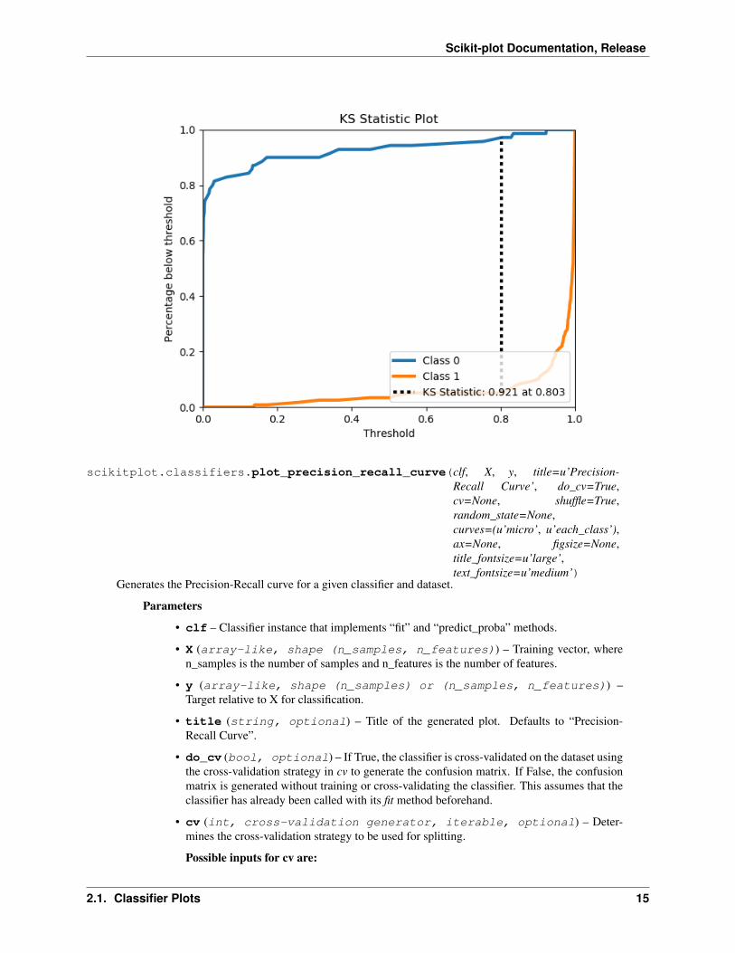
scikitplot.classifiers.plot_ks_statistic(clf, X, y, title=u’KS Statistic Plot’, do_cv=True,cv=None, shuffle=True, random_state=None,ax=None, figsize=None, title_fontsize=u’large’,text_fontsize=u’medium’)

Generates the KS Statistic plot for a given classifier and dataset.

Parameters




• title (string, optional) – Title of the generated plot. Defaults to “KS StatisticPlot”.



















Example

>>> lr = classifier_factory(LogisticRegression())>>> lr.plot_ks_statistic(X, y, random_state=1)<matplotlib.axes._subplots.AxesSubplot object at 0x7fe967d64490>>>> plt.show()



scikitplot.classifiers.plot_precision_recall_curve(clf, X, y, title=u’Precision-Recall Curve’, do_cv=True,cv=None, shuffle=True,random_state=None,curves=(u’micro’, u’each_class’),ax=None, figsize=None,title_fontsize=u’large’,text_fontsize=u’medium’)

Generates the Precision-Recall curve for a given classifier and dataset.

Parameters




• title (string, optional) – Title of the generated plot. Defaults to “Precision-Recall Curve”.













• curves (array-like) – A listing of which curves should be plotted on the resultingplot. Defaults to (“micro”, “each_class”) i.e. “micro” for micro-averaged curve







Example

>>> nb = classifier_factory(GaussianNB())>>> nb.plot_precision_recall_curve(X, y, random_state=1)<matplotlib.axes._subplots.AxesSubplot object at 0x7fe967d64490>>>> plt.show()



scikitplot.classifiers.plot_feature_importances(clf, title=u’Feature Impor-tance’, feature_names=None,max_num_features=20, or-der=u’descending’, ax=None, fig-size=None, title_fontsize=u’large’,text_fontsize=u’medium’)

Generates a plot of a classifier’s feature importances.

Parameters

• clf – Classifier instance that implements fit and predict_proba methods. The clas-sifier must also have a feature_importances_ attribute.

• title (string, optional) – Title of the generated plot. Defaults to “Feature impor-tances”.

• feature_names (None, list of string, optional) – Determines the feature names usedto plot the feature importances. If None, feature names will be numbered.

• max_num_features (int) – Determines the maximum number of features to plot. De-faults to 20.

• order ('ascending', 'descending', or None, optional) – Determinesthe order in which the feature importances are plotted. Defaults to ‘descending’.









Example

>>> import scikitplot.plotters as skplt>>> rf = RandomForestClassifier()>>> rf.fit(X, y)>>> skplt.plot_feature_importances(rf, feature_names=['petal length', 'petal width→˓',... 'sepal length', 'sepal width→˓'])<matplotlib.axes._subplots.AxesSubplot object at 0x7fe967d64490>>>> plt.show()



Clustering Plots

scikitplot.clustering_factory(clf)Takes a scikit-learn clusterer and embeds scikit-plot plotting methods in it.

Parameters clf – Scikit-learn clusterer instance

Returns The same scikit-learn clusterer instance passed in clf with embedded scikit-plot instancemethods.

Raises ValueError – If clf does not contain the instance methods necessary for scikit-plot in-stance methods.

scikitplot.clustering.plot_silhouette(clf, X, title=u’Silhouette Analysis’, met-ric=u’euclidean’, copy=True, ax=None,figsize=None, title_fontsize=u’large’,text_fontsize=u’medium’)

Plots silhouette analysis of clusters using fit_predict.

Parameters

• clf – Clusterer instance that implements fit and fit_predict methods.

• X (array-like, shape (n_samples, n_features)) – Data to cluster, wheren_samples is the number of samples and n_features is the number of features.

• title (string, optional) – Title of the generated plot. Defaults to “SilhouetteAnalysis”

• metric (string or callable, optional) – The metric to use when calculatingdistance between instances in a feature array. If metric is a string, it must be one of theoptions allowed by sklearn.metrics.pairwise.pairwise_distances. If X is the distance arrayitself, use “precomputed” as the metric.

• copy (boolean, optional) – Determines whether fit is used on clf or on a copy ofclf.







Example

>>> import scikitplot.plotters as skplt>>> kmeans = KMeans(n_clusters=4, random_state=1)>>> skplt.plot_silhouette(kmeans, X)<matplotlib.axes._subplots.AxesSubplot object at 0x7fe967d64490>>>> plt.show()

2.2. Clustering Plots 19


scikitplot.clustering.plot_elbow_curve(clf, X, title=u’Elbow Plot’, cluster_ranges=None,ax=None, figsize=None, title_fontsize=u’large’,text_fontsize=u’medium’)

Plots elbow curve of different values of K for KMeans clustering.

Parameters

• clf – Clusterer instance that implements fit and fit_predict methods and a scoreparameter.


• title (string, optional) – Title of the generated plot. Defaults to “Elbow Plot”

• cluster_ranges (None or list of int, optional) – List of n_clusters for which to plotthe explained variances. Defaults to range(1, 12, 2).










Example

>>> import scikitplot.plotters as skplt>>> kmeans = KMeans(random_state=1)>>> skplt.plot_elbow_curve(kmeans, cluster_ranges=range(1, 11))<matplotlib.axes._subplots.AxesSubplot object at 0x7fe967d64490>>>> plt.show()

2.2. Clustering Plots 21

CHAPTER 3

Functions API Reference

This document contains the stand-alone plotting functions for maximum flexibility. If you want to use factory func-tions clustering_factory() and classifier_factory(), use the Factory API Reference instead. Thismodule contains a more flexible API for Scikit-plot users, exposing simple functions to generate plots.

scikitplot.plotters.plot_learning_curve(clf, X, y, title=u’Learning Curve’, cv=None,train_sizes=None, n_jobs=1, ax=None,figsize=None, title_fontsize=u’large’,text_fontsize=u’medium’)

Generates a plot of the train and test learning curves for a given classifier.

Parameters



• y (array-like, shape (n_samples) or (n_samples, n_features)) –Target relative to X for classification or regression; None for unsupervised learning.

• title (string, optional) – Title of the generated plot. Defaults to “LearningCurve”








23


• train_sizes (iterable, optional) – Determines the training sizes used to plotthe learning curve. If None, np.linspace(.1, 1.0, 5) is used.

• n_jobs (int, optional) – Number of jobs to run in parallel. Defaults to 1.







Example

>>> import scikitplot.plotters as skplt>>> rf = RandomForestClassifier()>>> skplt.plot_learning_curve(rf, X, y)<matplotlib.axes._subplots.AxesSubplot object at 0x7fe967d64490>>>> plt.show()

24 Chapter 3. Functions API Reference


scikitplot.plotters.plot_confusion_matrix(y_true, y_pred, labels=None, ti-tle=None, normalize=False, ax=None,figsize=None, title_fontsize=u’large’,text_fontsize=u’medium’)

Generates confusion matrix plot for a given set of ground truth labels and classifier predictions.

Parameters

• y_true (array-like, shape (n_samples)) – Ground truth (correct) target val-ues.

• y_pred (array-like, shape (n_samples)) – Estimated targets as returned by aclassifier.

• labels (array-like, shape (n_classes), optional) – List of labels to in-dex the matrix. This may be used to reorder or select a subset of labels. If none is given,those that appear at least once in y_true or y_pred are used in sorted order. (new inv0.2.5)

• title (string, optional) – Title of the generated plot. Defaults to “ConfusionMatrix” if normalize is True. Else, defaults to “Normalized Confusion Matrix.

• normalize (bool, optional) – If True, normalizes the confusion matrix before plot-ting. Defaults to False.







Example

>>> import scikitplot.plotters as skplt>>> rf = RandomForestClassifier()>>> rf = rf.fit(X_train, y_train)>>> y_pred = rf.predict(X_test)>>> skplt.plot_confusion_matrix(y_test, y_pred, normalize=True)<matplotlib.axes._subplots.AxesSubplot object at 0x7fe967d64490>>>> plt.show()

25


scikitplot.plotters.plot_roc_curve(y_true, y_probas, title=u’ROC Curves’, curves=(u’micro’,u’macro’, u’each_class’), ax=None, figsize=None, ti-tle_fontsize=u’large’, text_fontsize=u’medium’)

Generates the ROC curves for a set of ground truth labels and classifier probability predictions.

Parameters


• y_probas (array-like, shape (n_samples, n_classes)) – Predictionprobabilities for each class returned by a classifier.

• title (string, optional) – Title of the generated plot. Defaults to “ROC Curves”.

• curves (array-like) – A listing of which curves should be plotted on the resultingplot. Defaults to (“micro”, “macro”, “each_class”) i.e. “micro” for micro-averaged curve,“macro” for macro-averaged curve









Example

>>> import scikitplot.plotters as skplt>>> nb = GaussianNB()>>> nb = nb.fit(X_train, y_train)>>> y_probas = nb.predict_proba(X_test)>>> skplt.plot_roc_curve(y_test, y_probas)<matplotlib.axes._subplots.AxesSubplot object at 0x7fe967d64490>>>> plt.show()

scikitplot.plotters.plot_ks_statistic(y_true, y_probas, title=u’KS Statistic Plot’,ax=None, figsize=None, title_fontsize=u’large’,text_fontsize=u’medium’)

Generates the KS Statistic plot for a set of ground truth labels and classifier probability predictions.

Parameters



27


• title (string, optional) – Title of the generated plot. Defaults to “KS StatisticPlot”.







Example

>>> import scikitplot.plotters as skplt>>> lr = LogisticRegression()>>> lr = lr.fit(X_train, y_train)>>> y_probas = lr.predict_proba(X_test)>>> skplt.plot_ks_statistic(y_test, y_probas)<matplotlib.axes._subplots.AxesSubplot object at 0x7fe967d64490>>>> plt.show()



scikitplot.plotters.plot_precision_recall_curve(y_true, y_probas, title=u’Precision-Recall Curve’, curves=(u’micro’,u’each_class’), ax=None, fig-size=None, title_fontsize=u’large’,text_fontsize=u’medium’)

Generates the Precision Recall Curve for a set of ground truth labels and classifier probability predictions.

Parameters



• curves (array-like) – A listing of which curves should be plotted on the resultingplot. Defaults to (“micro”, “each_class”) i.e. “micro” for micro-averaged curve





29




Example

>>> import scikitplot.plotters as skplt>>> nb = GaussianNB()>>> nb = nb.fit(X_train, y_train)>>> y_probas = nb.predict_proba(X_test)>>> skplt.plot_precision_recall_curve(y_test, y_probas)<matplotlib.axes._subplots.AxesSubplot object at 0x7fe967d64490>>>> plt.show()

scikitplot.plotters.plot_feature_importances(clf, title=u’Feature Importance’, fea-ture_names=None, max_num_features=20,order=u’descending’, ax=None, fig-size=None, title_fontsize=u’large’,text_fontsize=u’medium’)

Generates a plot of a classifier’s feature importances.

Parameters

• clf – Classifier instance that implements fit and predict_proba methods. The clas-sifier must also have a feature_importances_ attribute.



• title (string, optional) – Title of the generated plot. Defaults to “Feature impor-tances”.

• feature_names (None, list of string, optional) – Determines the feature names usedto plot the feature importances. If None, feature names will be numbered.

• max_num_features (int) – Determines the maximum number of features to plot. De-faults to 20.

• order ('ascending', 'descending', or None, optional) – Determinesthe order in which the feature importances are plotted. Defaults to ‘descending’.







Example

>>> import scikitplot.plotters as skplt>>> rf = RandomForestClassifier()>>> rf.fit(X, y)>>> skplt.plot_feature_importances(rf, feature_names=['petal length', 'petal width→˓',... 'sepal length', 'sepal width→˓'])<matplotlib.axes._subplots.AxesSubplot object at 0x7fe967d64490>>>> plt.show()

31


scikitplot.plotters.plot_silhouette(clf, X, title=u’Silhouette Analysis’, met-ric=u’euclidean’, copy=True, ax=None, figsize=None,title_fontsize=u’large’, text_fontsize=u’medium’)

Plots silhouette analysis of clusters using fit_predict.

Parameters

• clf – Clusterer instance that implements fit and fit_predict methods.


• title (string, optional) – Title of the generated plot. Defaults to “SilhouetteAnalysis”

• metric (string or callable, optional) – The metric to use when calculatingdistance between instances in a feature array. If metric is a string, it must be one of theoptions allowed by sklearn.metrics.pairwise.pairwise_distances. If X is the distance arrayitself, use “precomputed” as the metric.










Example

>>> import scikitplot.plotters as skplt>>> kmeans = KMeans(n_clusters=4, random_state=1)>>> skplt.plot_silhouette(kmeans, X)<matplotlib.axes._subplots.AxesSubplot object at 0x7fe967d64490>>>> plt.show()

scikitplot.plotters.plot_elbow_curve(clf, X, title=u’Elbow Plot’, cluster_ranges=None,ax=None, figsize=None, title_fontsize=u’large’,text_fontsize=u’medium’)

Plots elbow curve of different values of K for KMeans clustering.

Parameters

• clf – Clusterer instance that implements fit and fit_predict methods and a scoreparameter.

33



• title (string, optional) – Title of the generated plot. Defaults to “Elbow Plot”

• cluster_ranges (None or list of int, optional) – List of n_clusters for which to plotthe explained variances. Defaults to range(1, 12, 2).








Example

>>> import scikitplot.plotters as skplt>>> kmeans = KMeans(random_state=1)>>> skplt.plot_elbow_curve(kmeans, cluster_ranges=range(1, 11))<matplotlib.axes._subplots.AxesSubplot object at 0x7fe967d64490>>>> plt.show()



scikitplot.plotters.plot_pca_component_variance(clf, title=u’PCA ComponentExplained Variances’, tar-get_explained_variance=0.75,ax=None, figsize=None,title_fontsize=u’large’,text_fontsize=u’medium’)

Plots PCA components’ explained variance ratios. (new in v0.2.2)

Parameters

• clf – PCA instance that has the explained_variance_ratio_ attribute.

• title (string, optional) – Title of the generated plot. Defaults to “PCA Compo-nent Explained Variances”

• target_explained_variance (float, optional) – Looks for the minimumnumber of principal components that satisfies this value and emphasizes it on the plot. De-faults to 0.75.4





35




Example

>>> import scikitplot.plotters as skplt>>> pca = PCA(random_state=1)>>> pca.fit(X)>>> skplt.plot_pca_component_variance(pca)<matplotlib.axes._subplots.AxesSubplot object at 0x7fe967d64490>>>> plt.show()

scikitplot.plotters.plot_pca_2d_projection(clf, X, y, title=u’PCA 2-D Projection’, ax=None, fig-size=None, title_fontsize=u’large’,text_fontsize=u’medium’)

Plots the 2-dimensional projection of PCA on a given dataset. (new in v0.2.2)

Parameters

• clf – PCA instance that can transform given data set into 2 dimensions.

• X (array-like, shape (n_samples, n_features)) – Feature set to project,where n_samples is the number of samples and n_features is the number of features.

• y (array-like, shape (n_samples) or (n_samples, n_features)) –Target relative to X for labeling.



• title (string, optional) – Title of the generated plot. Defaults to “PCA 2-D Pro-jection”







Example

>>> import scikitplot.plotters as skplt>>> pca = PCA(random_state=1)>>> pca.fit(X)>>> skplt.plot_pca_2d_projection(pca, X, y)<matplotlib.axes._subplots.AxesSubplot object at 0x7fe967d64490>>>> plt.show()

37

CHAPTER 4

Indices and tables

• genindex

• modindex

• search

39


40 Chapter 4. Indices and tables

Python Module Index

sscikitplot.classifiers, 7scikitplot.clustering, 19scikitplot.plotters, 23

41


42 Python Module Index

Index

Cclassifier_factory() (in module scikitplot), 7clustering_factory() (in module scikitplot), 19

Pplot_confusion_matrix() (in module scikitplot.classifiers),

9plot_confusion_matrix() (in module scikitplot.plotters),

24plot_elbow_curve() (in module scikitplot.clustering), 20plot_elbow_curve() (in module scikitplot.plotters), 33plot_feature_importances() (in module scikit-

plot.classifiers), 17plot_feature_importances() (in module scikit-

plot.plotters), 30plot_ks_statistic() (in module scikitplot.classifiers), 13plot_ks_statistic() (in module scikitplot.plotters), 27plot_learning_curve() (in module scikitplot.classifiers), 7plot_learning_curve() (in module scikitplot.plotters), 23plot_pca_2d_projection() (in module scikitplot.plotters),

36plot_pca_component_variance() (in module scikit-

plot.plotters), 35plot_precision_recall_curve() (in module scikit-

plot.classifiers), 15plot_precision_recall_curve() (in module scikit-

plot.plotters), 29plot_roc_curve() (in module scikitplot.classifiers), 11plot_roc_curve() (in module scikitplot.plotters), 26plot_silhouette() (in module scikitplot.clustering), 19plot_silhouette() (in module scikitplot.plotters), 32

Sscikitplot.classifiers (module), 7scikitplot.clustering (module), 19scikitplot.plotters (module), 23

43

Scikit-plot Documentation

Documents

Transcript of Scikit-plot Documentation