
Scientific International Journal - SCPE
161
Scalable Computing: Practice and Experience Scientific International Journal for Parallel and Distributed Computing ISSN: 1895-1767 ⑦ ⑦ ⑦ ⑦ ⑦ ⑦ t Volume 21(1) March 2020
Transcript of Scientific International Journal - SCPE

Scalable Computing:Practice and Experience
Scientific International Journalfor Parallel and Distributed Computing
ISSN: 1895-1767
~~~~~~t
Volume 21(1) March 2020

Editor-in-ChiefDana PetcuComputer Science DepartmentWest University of Timisoaraand Institute e-Austria TimisoaraB-dul Vasile Parvan 4, 300223Timisoara, [email protected]
Managinig andTEXnical EditorSilviu PanicaComputer Science DepartmentWest University of Timisoaraand Institute e-Austria TimisoaraB-dul Vasile Parvan 4, 300223Timisoara, [email protected]
Book Review EditorShahram RahimiDepartment of Computer ScienceSouthern Illinois UniversityMailcode 4511, CarbondaleIllinois [email protected]
Software Review EditorHong ShenSchool of Computer ScienceThe University of AdelaideAdelaide, SA [email protected] TaliaDEISUniversity of CalabriaVia P. Bucci 41c87036 Rende, [email protected]
Editorial Board
Peter Arbenz, Swiss Federal Institute of Technology, Zürich,[email protected]
Dorothy Bollman, University of Puerto Rico,[email protected]
Luigi Brugnano, Università di Firenze,[email protected]
Giacomo Cabri, University of Modena and Reggio Emilia,[email protected]
Bogdan Czejdo, Fayetteville State University,[email protected]
Frederic Desprez, LIP ENS Lyon, [email protected] Fet, Novosibirsk Computing Center, [email protected] Fortino, University of Calabria,
[email protected] Goscinski, Deakin University, [email protected] Loulergue, Northern Arizona University,
[email protected] Ludwig, German Climate Computing Center and Uni-
versity of Hamburg, [email protected] Margenov, Institute for Parallel Processing and Bul-
garian Academy of Science, [email protected] Negru, West University of Timisoara,
[email protected] Ouedraogo, CRP Henri Tudor Luxembourg,
[email protected] Paprzycki, Systems Research Institute of the Polish
Academy of Sciences, [email protected] Trobec, Jozef Stefan Institute, [email protected] Vajtersic, University of Salzburg,
[email protected] R. Welch, Ohio University, [email protected] Zalewski, Florida Gulf Coast University,
SUBSCRIPTION INFORMATION: please visit http://www.scpe.org

Scalable Computing: Practice and ExperienceVolume 21, Number 1, March 2020
TABLE OF CONTENTS
Special Issue on Role of Scalable Computing and Data Analytics in Evolutionof Internet of Things:Introduction to the Special Issue 1
J.N. Swaminathan, Gopi Ram, Sureka Lanka
Brain Tumor Detection from MRI using Adaptive Thresholding andHistogram based Techniques 3
E. Murali, K. Meena
An Ensemble Integrated Security System with Cross Breed Algorithm 11Suresh Mundru, K. Meena
Background Modelling using a Q-Tree Based Foreground Segmentation 17S. Shahidha Banu, S. Maheswari
Topological ordering Signal Selection Technique for Internet of Thingsbased Devices using Combinational Gate for Visibility Enhancement 33
Agalya Rajendran, Muthaiah Rajappa
Secured Identity Based Cryptosystem Approach for Intelligent RoutingProtocol in VANET 41
A. Karthikeyan, P.G. Kuppusamy, Iraj S. Amiri
An Application based Efficient Thread Level Parallelism Scheme onHeterogeneous Multicore Embedded System for Real Time ImageProcessing 47
K. Indragandhi, P.K. Jawahar
A Study to Analyze Enhancement Techniques on Sound Quality forBone Conduction and Air Conduction Speech Processing 57
Putta Venkata Subbaiah, Hima Deepthi V.
A Novel Approach Based on Modified Cycle Generative AdversarialNetworks for Image Steganography 63
P.G. Kuppusamy, K.C. Ramya, S. Sheeba Rani, M. Sivaram,Vigneswaran Dhasarathan
Minimizing Deadline Misses and Total Run-time with Load Balancingfor a Connected Car Systems in Fog Computing 73
K. Jairam Naik, D. Hanumanth Naik

Long and Strong Security using Reputation and ECC for CloudAssisted Wireless Sensor Networks 85
D. Antony Joseph Rajan, E.R. Naganathan
Detection and Classification of 2D And 3D Hyper Spectral ImageUsing Enhanced Harris Corner Detector 93
S. Pavithra, A. Karthikeyan, P.M. Anu
SPCACF: Secured Privacy-Conserving Authentication Scheme usingCuckoo Filter in VANET 101
A. Rengarajan, M. Mohammed Thaha
Logistics Optimization in Supply Chain Management using ClusteringAlgorithms 107
R. Mahesh Prabhu, M.S. Hema, Srilatha Chepure, M. Nageswara Guptha
Acoustic Feedback Cancellation in Efficient Hearing Aids using GeneticAlgorithm 115
G. Jayanthih, Latha Parthiban
Analysis on Deep Learning methods for ECG based CardiovascularDisease Prediction 127
S. Kusuma, J. Divya Udayan
A Hybrid Intrusion Detection System for Mobile Adhoc Networksusing FBID Protocol 137
D. Rajalakshmi, K. Meena
Regular Papers:
Monte Carlo Simulations of Coupled Transient Seepage Flow and SoilDeformation in Levees 147
Fred Thomas Tracy, Jodi L. Ryder, Martin T. Schultz, Ghada S. Ellithy,Benjamin R. Breland, T. Chris Massey, Maureen K. Corcoran
© SCPE, Timişoara 2020

Scalable Computing: Practice and Experience, ISSN 1895-1767, http://www.scpe.org© 2020 SCPE. Volume 21, Issue 1, pp. 1–2, DOI 10.12694:/scpe.v21i1.1576
INTRODUCTION TO THE SPECIAL ISSUE ON ROLE OF SCALABLE COMPUTINGAND DATA ANALYTICS IN EVOLUTION OF INTERNET OF THINGS
J.N. SWAMINATHAN∗, GOPI RAM†, AND SUREKA LANKA‡
The evolution of Internet of Things has given way to a Smart World where there is an improved integrationof devices, systems and processes in humans through all pervasive connectivity. Anytime, anywhere connectionand transaction is the motto of the Internet of things which brings comfort to the users and sweeps the problemof physical boundary out of the way. Once it has come into the purview of developers, new areas have beenidentified and new applications have been introduced. Small wearables which can track your health to bigautomated vehicles which can move from one place to another self navigating without human intervention arethe order of the day. This has also brought into existence a new technology called cloud, since with IoT comesa large number of devices connected to the internet continuously pumping data into the cloud for storage andprocessing. Another area benefited from the evolution of IoT is the wireless and wired connectivity through awide range of connectivity standards.
As with any technology, it has also created a lot of concerns regarding the security, privacy and ethics.Data protection issues created by new technologies are a threat which has been recognized by developers, publicand also the governing body long back. The complexity of the system arises because of the various sensors andtechnologies which clearly tell the pattern of the activities of the individual as well an organization making usthreat prone. Moreover, the volume of the data in the cloud makes it too difficult to recognize the privacyrequirement of the data or to segregate open data from private data. Data analytics is another technology whichsupposedly increases the opportunity of increasing business by studying this private data collected from IoTand exploring ways to monetize them. It also helps the individual by recognizing their priorities and narrowingtheir search. But the data collected are real world data and aggregation of this data in the cloud is an openinvitation to the hackers to study about the behaviors of the individuals.
The special issues of Scalable Computing has attract related to the Role of Scalable Computing and DataAnalytics in Evolution of Internet of Things has attracted 28 submissions from which were selected 12. In whatfollows we present them shortly:
1. Murali et. al has executed on detecting brain tumor using thresholding and histogram techniques.2. Suresh et. al has introduced an ensemble integrated security system with cross breed technique.3. Shahidha Bhanu has done background modeling using a Q-Tree based foreground segmentation.4. Agalya et. al has executed topological ordering signal selection techniques for iot based devices. The
work has been funded under dst-inspire program.5. Karthikeyan et. al has introduced secured identity based cryptosystem approach for intelligent routing
protocol in vanet.6. Indragandhi et.al has developed an application based ETLP scheme on heterogeneous multicore em-
bedded system for real time image processing.7. Putta Venkata Subbaiah et.al has done a study to analyze enhancement techniques on sound quality
for bone conduction and air conduction speech processing.8. Kuppusamy et.al has introduced a novel approach based on modified cycle generative adversarial net-
works for image steganography.
∗QIS College of Engineering and Technology, Ongole, Andhra Pradesh, India†National Institute of Technology, Warangal, Telangana, India‡Stamford International University, Bangkok, Thailand.
1

9. Jairam Naik et.al has executed minimizing deadline misses and total run-time with load balancing fora connected car systems in fog computing.
10. Antony Joseph Rajan et. al has proposed long and strong security using reputation and ecc for cloudassisted wireless sensor networks.
11. Pavithra et. al has detected and classified 2D and 3D hyper spectral image using enhanced harriscorner detector.
12. Rengarajan et. al has proposed secured privacy-conserving authentication scheme using cuckoo filterin vanet.
13. Hema et. al has introduced logistics optimization in supply chain management using clustering algo-rithms.
14. Jayanthi et. al has executed acoustic feedback cancellation in efficient hearing aids using geneticalgorithm.
15. Kusma et. al has analysed on deep learning methods for ECG based cardiovascular disease prediction.16. Finally Rajalakshmi et. al has introduced a hybrid intrusion detection system for mobile adhoc networks
using fbid protocol.
Acknowledgement: The Guest editorial members want to acknowledge Dr. N. S. Kalyan Chakravarthy,Chairman & Correspondent, QIS Group of Institutions, Ongole, Andhra Pradesh.
2

Scalable Computing: Practice and Experience, ISSN 1895-1767, http://www.scpe.org© 2020 SCPE. Volume 21, Issue 1, pp. 3–10, DOI 10.12694:/scpe.v21i1.1600
BRAIN TUMOR DETECTION FROM MRI USING ADAPTIVE THRESHOLDINGAND HISTOGRAM BASED TECHNIQUES
E. MURALI∗AND K. MEENA†
Abstract. This paper depicts a computerized framework that can distinguish brain tumor and investigate the diverse highlightsof the tumor. Brain tumor segmentation means to isolated the unique tumor tissues, for example, active cells, edema and necroticcenter from ordinary mind tissues of WM, GM, and CSF. However, manual segmentation in magnetic resonance data is a time-consuming task. We present a method of automatic tumor segmentation in magnetic resonance images which consists of severalsteps. The recommended framework is helped by image processing based technique that gives improved precision rate of thecerebrum tumor location along with the computation of tumor measure. In this paper, the location of brain tumor from MRI isrecognized utilizing adaptive thresholding with a level set and a morphological procedure with histogram. Automatic brain tumorstage is performed by using ensemble classification. Such phase classifies brain images into tumor and non-tumors using FeedForwarded Artificial neural network based classifier. For test investigation, continuous MRI images gathered from 200 people areutilized. The rate of fruitful discovery through the proposed procedure is 97.32 percentage accurate.
Key words: MRI, Morphological, Thresholding, Brain tumor, Level set, Histogram
AMS subject classifications. 92B20, 68U10
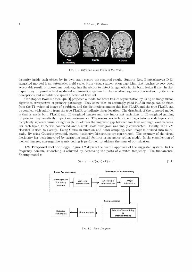
1. Introduction. One of the necessary steps in most of the medical imaging analysis is to extract theboundary of a locality of our interest. Precise location is vital in cerebrum tumor identification. The level ofexactness can be expanded through the use of computer aided system. Such framework can assist the radiologistwith detecting brain tumor all the more properly. Magnetic resonance image have been extensively approvedfor imaging because of its competences are generating precise brain scan in less interval time, with changingcontrasts, such as T1-weighted, T2-weighted and Flair. Respectively difference yields intensity dissimilaritiesin MRI scans. Cerebrum is a 3-D composite structure. Numerous views of brain images are axial, sagittal andcoronal. In axial view the brain image was divided by a horizontal plane. The sagittal view, the brain image isdivided into right and left part of the median plane and in coronal view, the brain is divided into ventral anddorsal by frontal plane. Figure 1.1 shows views of MRI brain scan.
Image enhancement techniques are used to develop the image feature for human perception. They aredefined as methods of image processing such that, the result is more appropriate than the original image.Histogram equalization is a fundamental tool in image enhancement. It is likely to aid in perceptive of howthey function on digital images. The equalization of intensity level method is an enhanced image with dynamicrange, which will tend to have high difference. The increased in contrast is owing to the circumstance that theaverage intensity level of the equalized image is enhanced by the original. Overall, the increased in intensity isdue to the reality that the average intensity level in the equalized image histogram is better than the original.
1.1. Related work. Mouli Laha [1] introduced an approach that embedded iterative thresholding inparallel to Otsu’s global threshold. There is no need to set any limit value before the procedure. Similarly, thecropping skull stripped techniques from brain scan is efficient for three views. This method operates very wellin the case of 2D.
K Sudharani and T.C Sarma [2] proposed an algorithm that calculates the threshold qualitatively andquantitatively by methods of the standard images. It diminishes misclassification errors where the insignificant
∗Research Scholar, Vel Tech Rangarajan Dr.Sagunthala R&D Institute of Science and Technology, Avadi, Chennai, India.†CSE Department, Professor, Vel Tech Rangarajan Dr.Sagunthala R&D Institute of Science and Technology, Avadi, Chennai,
India
3
4 E. Murali, K. Meena
Fig. 1.1. Different angle Views of the Brain.
disparity inside each object by its own can’t ensure the required result. Sudipta Roy, Bhattacharyya D [3]suggested method is an automatic, multi-scale, brain tissue segmentation algorithm that reaches to very goodacceptable result. Proposed methodology has the ability to detect irregularity in the brain lesion if any. In thatpaper, they proposed a level set-based minimization system for the variation segmentation method by iterativeperceptions and mutable the speed function of level set.
Christopher Bowels, Chen Qin [4] proposed a model for brain tissues segmentation by using an image fusionalgorithm, irrespective of primary pathology. They show that an seemingly good FLAIR image can be fusedfrom the T1-weighted image of a subject, and the distinctions among this fake FLAIR and the true FLAIR canbe coupled with validity from the true FLAIR to indicate tissue location. The drawback of the proposed modelis that is needs both FLAIR and T1-weighted images and any important variations in T1-weighted gainingproprieties may negatively impact on performance. The researchers isolate the images into n- scale layers withcompletely separate visual categories [5] to address the linguistic gap between low level and high level features.For each layer, FDA was conducted and a multi scale histogram was finally constructed. Finally, the SVMclassifier is used to classify. Using Gaussian function and down sampling, each image is divided into multi-scale. By using Gaussian pyramid, several distinctive histograms are constructed. The accuracy of the visualdictionary has been improved by extracting spatial features using sparse coding model. In the classification ofmedical images, non-negative scanty coding is performed to address the issue of optimization.
1.2. Proposed methodology. Figure 1.2 depicts the overall approach of the suggested system. In thefrequency domain, smoothing is achieved by decreasing the parts of elevated frequency. The fundamentalfiltering model is
G(u, v) = H(u, v) · F (u, v) (1.1)
Fig. 1.2. Flow Diagram

Brain Tumor Detection from MRI using Adaptive Thresholding and Histogram based Techniques 5
The image was filtered with Fourier transform F (u, v) and filtered function is H(u, v). From that point onward,gray level normalization is connected to change the scope of the pixel intensity. By utilizing anisotropic diffusionfilter to diminish the image noise without evacuating critical parts of the image content, commonly edges, linesor different subtleties that is vital for the elucidation of the image. By using imsubtract, features are subtractfrom one image from another image, or to subtract a constant value from an image. Imsubtract subtracts eachpixel value from the comparing pixel in the other input image in one of the input image and returns the resultin the related pixel in the output image.
In adaptive thresholding modifications the threshold is dynamically over the image. Thresholding commonlytakes a grayscale or colour image as an input and, in the least complex usage, yields a binary image speakingto the segmentation. The process of shape analysis consists of two main steps: (1) the extraction of imagecomponents of the target (e.g., area, boundary, network pattern and skeleton), (2) the description of the shapefeatures (e.g., size, perimeter, circularity and compactness) and finally show the detected tumor area.
1.3. Organization of the paper. This paper is organized as follows. Section 1 describes the introduction,literature review and block diagram of the proposed method. Section 2 shows the various methodologies such asHistogram Method, Adaptive Threshold, Anisotropic Diffusion filtering and Level set method in detail. Section3 presents the experimental results and discussion. Section 4 concludes the paper.
2. Methodology. The algorithm introduced in this section is performed by an automatic thresholdingmethod in its place of physically changing the threshold for each image. The threshold range is done automat-ically dependent on the mean and standard deviation of every area among four sub regions.
2.1. Histogram Method. This technique is used to convert the input image into a gray image. Ahistogram equalization technique has been connected to this grayscale image to enhance the intensity imagecontract, which aids to recognize the brightest portion of the image. Before applying adaptive thresholdingwith ostu value 0.31, we shift just over white pixels into full white and others into dark ones. The image isconverted to binary after that, morphological dilation and erosion with basic component of [1;1;1] that hasbetter segmentation was implemented at that point. The pixels less than 250 pixels have been expelled as thisprecisely portioned the districts of the tumor. At long last tumor area is recognized. The histogram strategy forordering a pixel-by-pixel image characterizes single or multiple thresholds. A fundamental way to determiningthe threshold value T is by studying the histogram for maximum values and fining the smallest point, typicallybetween two consecutive maximum values of histograms. The statistics method will provide a good result,when a histogram is bi-modal. By equating the gray value of each pixel with the specified threshold T , a pixelcan be classified into one or two classes. An image f(x, y) may be split into two classes by a gray value limit T .
g(x, y) =
{1, if f(x, y) > T
0, if f(x, y) ≤ T(2.1)
Here g(x, y) is the segmented image with two binary values “1” and “0” and T is the threshold assigned to thesmallest point between two histogram peak values.
2.2. Adaptive Threshold. Thresholding is entitled adaptive since a different type of threshold is used fordifferent regions in the image. Thresholding expect that the image has pixel values generally different from thebackground. This technique approves the threshold value T to alternate depending on the image’s progressivelydifferent function characteristics. Threshold T relies on the coordinated spatial (x, y) itself. This technique isadapted with some optimization. Following is the outline of adaptive thresholding:
1. Binarizing the image with a single threshold T ;2. Thinning the threshold image;3. Remove all branch points in the thin image;4. All remaining endpoints are located in the analysis queue and used as an initial point for tracking;5. Track the region with threshold T6. If the region has passed, T = T − 1, go to 5
The adaptive thresholding algorithm used a recursive filter to determine the nearby weighted mean in theimage just along the row, or set of rows. Here, to calculate the local mean, we use symmetrical 2D Gaussian

6 E. Murali, K. Meena
Fig. 2.1. Histogram Equilization with White Pixels
smoothing. This is slower yet gradually wide. Median filtration is an alternative to the mean and offers theoption to use a fixed threshold relative to the mean / median.
Let fs(n) is the sum of the s pixel values at point n.The resulting T (n) is either 1 or 0 depending on whether it is t percent darker than the previous s pixels
average value.
g(x, y) =
1, if Pn <(fs(n)
s
)(100− t100
)0, otherwise
(2.2)
2.3. Anisotropic Diffusion filtering. In order to lighten the noise effects, noise reduction is frequentlyused before segmentation, characterization and recognition to expel or lessen the noise. Noise reduction is animportant approach for image processing that has broad implementation in various areas [7, 8]. The key is todecrease the noise without breaking down the vital highlights in the image. In this way, noise decrease hastwo objectives. One is to expel the noise from the image, and the other is to save the imperative highlights,for example, the edges in the image. A uproarious image can frequently be shown as one of the two modelsdepending on the type of noise: a linear model and a nonlinear model. A MR image is commonly demonstratedas a noise model.
The anisotropic diffusion filtering is a general scale space way to deal with edge detection presented byPerona and Malik. In their work they moved from the linear scale-space model which considers the filteredimage I(x, y, t) and unique image Io(x, y) implanted in a novel group of functions characterized by
I(x, y, t) = Io(x, y) ·G(x, y, t) (2.3)
The simple equation of anisotropic diffusion as presented in [5] is
∂I(x, y, t)
∂t= div[g(|∆I(x, y, t)|)∆I(x, y, t)] (2.4)
where t is the time parameter, the original image is I(x, y, 0), the gradient of the image version at the time t,and the so-called conductivity function is g.
2.4. Level set method. Interested object’s rough boundaries are divided by thresholding method. Theextracted portion is regarded as a level-set method initialization [9]. Methods of level-sets rely on partialdifferential equation to the surfaces of model deformation. Level sets techniques rely on two key embeddingtechniques; first, the implantation of the surface as the zero level set of a greater velocity to this greater pointset feature. A level set equation represents the assessment of the shape or surface. The solution to which this

Brain Tumor Detection from MRI using Adaptive Thresholding and Histogram based Techniques 7
partial differential equation tends is calculated iteratively by updating at each interval of moment, below isshown the overall form of the level set equation:
∂φ
∂t= −|∆φ| · F (2.5)
Here, F is the frequency that defines the assessment of the level set. By using F , given a specific initializationof the level set function, we can guide the level set to the different areas or shapes. It is also essential to havean initial mask for the level set function, which can take the form of a two-dimensional square or any otherclosed form. In this article, threshold findings act as a seed for a level-set method and the final tumor regionis acquired after a few iterations.
2.5. Feed Forward Artificial Neural network. Feed forward Artificial Neural Network One of thesimplest feed forward neural networks (FFNN, consists of three layers: an input layer, hidden layer and outputlayer. In each layer there are one or more Processing Elements (PEs). PEs is meant to simulate the neuronsin the brain and this is why they are often referred to as neurons or nodes. PE receives inputs from either theoutside world or the previous layer. There are connections between the PEs in each layer that have a weight(parameter) associated with them. This weight is adjusted during training. Information only travels in theforward direction through the network -there are no feedback loops.
3. Results and discussion.
3.1. Performance evaluation. Table 3.1 gives the details of the tumor are present along with the locationof it in the brain according the hemispheres of the brain.
The following performance metrics are used to evaluate the efficiency of the proposed algorithm.
True Positive (TP ) = the no. of images correctly identified as tumorTrue Negative (TN) = the no. of images correctly identified as healthyFalse Negative (FN) = the no. of images incorrectly identified as healthy.False Positive (FP ) = the no. of images incorrectly identified as tumor.
Table 3.1Tumor segmentation and its location
Input Image Histogram Equalization Tumor Outline Brain Area (B) Tumor Area(T) Ratio(B/T)
12046 114 0.946
24283 1435 5.90
1523 98 0.639
21652 1142 5.274
32970 848 2.572
126793 3368 12.570

8 E. Murali, K. Meena
Fig. 3.1. Tumor detection using level set and bounding box with bias corrected image
Accuracy: It is a measure of the closeness of the measurements to true value
Accuracy =
∑(TP + TN)∑
(TP + TN + FN + FP )× 100 (3.1)
Precision: It is definite as the accuracy as the combination of both actuality and exactness
Precision =
∑(TP )∑
(TP + FP )× 100 (3.2)
3.2. Results. In this module, the suggested structure is the detection of tumor slices in which the bound-ary box is situated around the tumor and acts as a seed for brain tumor segmentation (Figure 3.1). Thealgorithm set threshold and level set is used to obtain the accurate tumor.
Table 3.2 shows the segmentation of the image with delta value is 0.1429 and different threshold value forthe different images.
Table 3.2Performance of brain tumour segmentation based on three evaluation indexes
Subject Density ThresholdP1 0.0745 0.3725P2 0.0487 0.2196P3 0.7941 0.2588P4 0.0961 0.2471: : :: : :: : :: : :
P212 0.1669 0.1569Mean 0.2869 0.2492Std 0.0141 0.0123

Brain Tumor Detection from MRI using Adaptive Thresholding and Histogram based Techniques 9
Table 3.3Performance of brain tumour segmentation
Subject TP TN FP FN Precision RecallP1 1 0 0 0 1 1P2 1 0 0 0 1 1P3 1 0 0 0 1 1P4 1 0 0 0 1 1: : : : : : :: : : : : : :: : : : : : :: : : : : : :
P212 1 0 0 0 1 1Total 212 182 25 0 5 99.52 98.87
Table 3.4Performance of the proposed system
Total Number of Images TP TN FP FN Sensitivity Specificity Accuracy212 182 25 0 5 97.76 100 97.32
Of the 187 images taken with the tumor, 182 images were evaluated by the framework efficiently. Other5 images are incorrectly acknowledged without a tumor. The reason for this failure was that there is no cleardifference in pixel intensity between the tumor region and the rest of the brain. The framework correctlyrecognized 25 images without a tumor as images without a 100 percent successful tumor. The outcome of thesuggested framework is shown in Table 3.4.
As discussed above, segmentation of brain tumour plays an important role in diagnostic procedures. Theaccurate segmentation helps in clinical diagnostic, but also helps to increase the lifetime of the patient. Basedon the conventional histogram equalization algorithm, the paper presented an adaptive gray level mappingalgorithm which takes the entropy and visual effects as the target function. The selection rule of parameter indifferent conditions and the identification method of the image gray type are also presented. The result showsthat the implemented method helps in detection of enhancing tumour as well as specifying tumour to the actualtumour region only.
4. Conclusion. In identifying tumor tissues in the medicine sector, this paper suggested an outstandingand innovative classification of brain image. The paper provided an adaptive gray level mapping algorithmbased on the histogram equalization algorithm that takes entropy and visual effects as the target function. Theenhanced images are reconfigured using histogram equalization to reconfigure their pixel levels in histogramtechniques. Developing more suitable techniques for detecting malignant brain tumors that are tiny in sizewould be excellent. The real tumor size can also be calculated from the 3D image.
REFERENCES
[1] Mouli Laha, Prasun Chandra Tripathi, and Soumen Bag, A Skull stripping from brain MRI Using Adaptive Iterativethresholding and Mathematical Morphology,recent advances in Information Technology RAIT-2018.
[2] K Sudharani, T.C. Sarma and K Satya Prasad , Histogram related threshold techniques for region based automatic braintumor detection,Indian journal of science and technology, dec-2016.
[3] Sudipta Roy, Bhattacharyya D, Samir kumar and Taihoon Kim, An iterative implementation of level set for precisesegmentation of brain tissues and abnormality detection from MR Images,IETE Journal of Research, June 2017.
[4] Christopher Bowles, Chen Qin, Ricardo Guerrero, Roger Gunn, and David Alexander Dickie, Brain lesion seg-mentation through image synthesis and outlier detection, Neuro Image: clinical Elsevier 2017.
[5] Zhang, R., Shen, J., Wei, F., Li, X., and Sangaiah, A. K, LU-Medical image classification based on multi-scale non-negative sparse coding, Artif. Intell. Med., 2017. https://doi.org/10.1016/j.artmed.2017. 05.006

10 E. Murali, K. Meena
[6] Chourmouzios Tsiotsios and Maria Petrou, On the choice the parameter for anisotropic diffusion in image processing,Pattern recognition in Elsevier, 2012.
[7] G. Gerig, O. Kubler, R. Kikinis, and F. A. Jolesz, Nonlinear anisotropic filtering of MRI data, IEEE Transactions onMedical Imaging, vol. 11, no. 2, pp. 221–232, 1992.
[8] J. Tang, S. Millington, S. T. Acton, J. Crandall, and S. Hurwitz, Surface extraction and thickness measurement ofthe articular cartilage from MR images using directional gradient vector flow snakes, IEEE Transactions on BiomedicalEngineering, vol. 53, no. 5, pp. 896–907, 2006.
[9] C. Li. R. Huang, Z. Ding, J. Chris Gatenby, N. Dimtris Metaxas, A level set method for Image segmentation in thePresence of Intensity in homogeneities with application to MRI, IEEE transactions on image processing, vol.20, No. 7,July 2011.
[10] M.H.O. Rashid, M.A Mamun, M.A Hossain and M.P Uddin, Brain tumor detection using Anisotropic Filtering SVM Clas-sifier and Morphologival Operation from MR Images, International conference on Computer, Communication, Chemical,Materials and Electronics Engineering, Feb 2018.
[11] H.R. Shahdoosti, A. Mehrabi, MRI and PET image fusion using structure tensor and dual ripplet-II transform, Multimed.Tools Appl. 77 (17) (2017)22649–22670.
[12] G. Litjens et al., A survey on deep learning in medical image analysis, Med. Image Anal., vol. 42, pp. 60–88, Dec. 2017.[13] X. Zhao, Y. Wu, G. Song, Z. Li, Y. Zhang, and Y. Fan, A deep learning model integrating FCNNs and CRFs for brain
tumor segmentation,Med. Image Anal., vol. 43, pp. 98–111, Jan. 2017.[14] M. Havaei et al., Brain tumor segmentation with deep neural networks, Med. Image Anal., vol. 35, pp. 18–31, Jan. 2017.[15] S. Pereira, A. Pinto, V. Alves, and C. A. Silva, Brain tumor segmentation using convolutional neural networks in MRI
images,IEEE Trans.Med. Image vol. 35, no. 5, pp. 1240–1251, May 2016
Edited by: Swaminathan JNReceived: Sep 3, 2019Accepted: Nov 30, 2019

Scalable Computing: Practice and Experience, ISSN 1895-1767, http://www.scpe.org© 2020 SCPE. Volume 21, Issue 1, pp. 11–15, DOI 10.12694:/scpe.v21i1.1602
AN ENSEMBLE INTEGRATED SECURITY SYSTEMWITH CROSS BREED ALGORITHM
SURESH MUNDRU∗AND K. MEENA†
Abstract. Blockchain and IoT are two technologies are most widely popular in present scenario, but technologies are morecomplicated. The blockchain used to transforms storage and data analysis. In recent years, the blockchain is at the heart ofcomputer technologies. It is a cryptographically secure distributed database technology for storing and transmitting information.Various attacks are done in many networks. Many research articles discussed about the security issues over the IoT based secureusing block chain technology. In this paper, an Ensemble Integrated Security System (EISS) is introduced to improve the securityfor the heterogeneous network which consists of normal and abnormal nodes which is processed with the block chain, IoT. Resultsshow the performance of the OUATH-2 and EISS algorithm.
Key words: Blockchain, Internet of things, Networks.
AMS subject classifications. 68M11, 68M10
1. Introduction. Security is most widely used in many applications. In routing protocols it is veryimportant to secure the routing. If the WSN is integrated with IoT and blockchain it becomes more compatiblefor security. IoT is the fast-growing technology in the present world [1]. In 2015, i.e., around 20 years afterthe term was authored, the IEEE IoT Initiative discharged a report whose principle objective was to set upa benchmark meaning of the IoT, with regards to applications extending from little, confined frameworksobliged to a particular area, to enormous worldwide frameworks made out of complex sub-frameworks thatare geologically circulated [2]. In this archive, we can discover an outline of the IoT’s design necessities,its empowering advancements, just as a brief meaning of the IoT as an ”application space that incorporatesdistinctive innovative and social fields”. At its center, the IoT comprises of arranged items that sense andassemble information from their environment, which is then used to perform robotized capacities to helphuman clients. The IoT is still relentlessly developing around the world, on account of extending Internetand remote access, the presentation of wearable gadgets, the falling costs of installed PCs, the advancementof capacity innovation and distributed computing [3]. Today, the IoT pulls in a large number of research andmodern interests. As time passes, littler and more intelligent gadgets are being executed in numerous IoT areas,including lodging, exactness agribusiness, foundation observing, individual medicinal services, and independentvehicles just to give some examples.
Blockchain is the technology which is used to improve the performance in terms of security. Users can usevarious private and public keys to solve the security issues to transfer the data. The most serious issue withIoT security is that ”there is no most concerning issue [4] [5] [6].” IoT has more mind-boggling details thanconventional data innovation (IT) framework. It is significantly more liable to comprise of different equipmentand programming items. As indicated by Forrester senior investigator Merit Maxim, the three primary regionsof IoT security are a gadget, arrange, and back-end, which can all be objective and we ought to be cautiousabout.
Providing security for the IoT and nodes in the Network. In this paper, an ensemble integrated securitysystem (EISS) is introduced to provide security between the nodes. To improve the performance of the security
∗Research Scholar, Vel Tech Rangarajan, Dr. Sagunthala R&D Institute of Science and Technology,Chennai-600062, India. &Assistant Professor, CSE Department, KKR&KSR Institute of Technology and Sciences, Andhra Pradesh, India.
†Professor, CSE Department, Vel Tech Rangarajan, Dr.Sagunthala R & D Institute of Science and Technology, Chennai-600062,India.
11

12 S. Mundru, K. Meena
Fig. 1.1. Architecture Diagram for EISS
within the nodes which are integrated with IoT and blockchain. All the domains are integrated and calledas EISS.
2. Problem Statement. The present problem is addressed in IOT devices is security. Many routingprotocols have the problem with security and certainty. Many researches have been done on providing securityand predictable issues with IOT and routing protocols. Blockchain is updated technology to improve thesecurity in IOT and routing protocols.
3. Releated Work. A basic security challenge of the IoT originates from its consistently extending edge.In an IoT arrange, hubs at the edge are potential purposes of disappointment where assaults, for example,Distributed Denial-of-Service (DDoS) can be propelled [7]. Inside the IoT edge, a lot of adulterated hubs andgadgets can act together to fall the IoT administration arrangement, as observed as of late in botnet attacks [8].
A main issue of disappointment not exclusively is a danger to accessibility, yet additionally to classifica-tion and approval [9]. A concentrated IoT does not give worked in ensures that the specialist co-op won’tabuse or alter clients IoT information. Besides, classification assaults emerge from personality parodying anddissecting directing and traffic data. In an information driven economy, ensures are important to anticipatemisappropriation of IoT information.
IoT faces classification assaults that emerge from character parodying and examining steering and trafficdata, just as uprightness assaults, for example, change assaults and Byzantine directing data assaults [10]. In-formation honesty in the incorporated IoT arrangement is tested by infusion assaults in applications where basicleadership depends on approaching information streams. IoT information modification, information burglaryand personal time can bring about shifting degrees of misfortune. Guaranteeing security is vital in a frameworkwhere keen gadgets are required to connect self-ruling and take part in financial exchanges. Current securityarrangements in the IoT are incorporated, including outsider security administrations. Utilizing blockchains forsecurity strategy implementation and keeping up openly auditable record of IoT connections, without relyingupon an outsider, can demonstrate to be profoundly beneficial to the IoT.
IoT frameworks produce huge volumes of information that require arrange network and power, preparingand capacity assets to change this information into significant data or administrations. Close to dependableavailability and system versatility, digital security and information protection of are significant significance inutilizing IoT systems. Right now, unified engineering models broadly used to validate, approve and interfacevarious hubs in an IoT organize. With the developing number of gadgets to many billions, incorporatedframeworks will separate and bomb when they brought together server winds up inaccessible. DecentralizedIoT design was proposed to understand this issue, wherein it moves away a portion of the system handling

An Ensemble Integrated Security System with Cross Breed Algorithm 13
assignments to the edge [11]. For example, in haze registering models, a portion of the basic activities thatused to be handled by cloud servers are currently relegated to be performed by IoT centers or haze [12].Distributed (P2P) engineering gives another arrangement, where neighbouring gadgets legitimately connectwith one another in lattices to distinguish, verify and trade data without utilizing any incorporated hub oroperator between them [13].
4. Block Chain. The blockchain, consists of a chain of blocks. In every block, the data structure is allowedto blockchain to save the transactions done on every block which is linked to the chain by cryptography. Inblockchain there are basic fundamental attributes such as Saved, transparent, and decentralized [14]. Everytransaction in blockchain is safely and communicate with each other based on the trust-less method, i,e thereis no need to believe another device and third parties. Especially in this paper, the blockchain technology isused to save every data into the each block and uses the encryption and decryption with the key. It is verypowerful to use the algorithm for security.
5. An Ensemble Integrated Security System (EISS). This section explains about the functionalityof the Encryption and decryption algorithm and how the IoT and blockchain are integrated in this. RSA is avery efficient and fast encryption algorithm that is used for securing data with the public-key. In this scenario,RSA is used to provide security at every node which is integrated with blockchain and generates a key for everyblock. Maintaining the secret keys at the block level is very difficult. The key generation is also very fast forevery block and this also maintains the large data at every block. At the network setup, the integration of RSAand blockchain is implemented with the efficient network setup and security. The total no of nodes within thenetwork is based on the data allowed at every node. The integrated system is implemented at network.
The integration of RSA and Block chain at every network is formalized by:KeyGen:(E, q, a, b,G, n, h; d,Q)
whereE is variable with elliptic curve
y2 = x3 + ax+b
Fq(5.1)
q is prime2256 − 232 − 29 − 28 − 27 − 26 − 24 − 1 (5.2)
while a, b : a = 0, b = 7G,n : consider random base point in E with prime order n.h: hash, instantiated with SHAISigning key: d = [1, n− 1]Verification key: Q = dG ∈ ESign(d : m):
(r, s) ∈ F 2 (5.3)where:r is the non-zero x-coordinator of point kG for some k←[1,n-1]s :
s = k−1(hm+ d · r) mod n (5.4)Verify (Q; r, s) : (s, s ∈ [1, n− 1]) and (v = r), where v=the x-coordinator of pointThe hash function used is defined with parameters x, y and z.The equation is to find the 2y numbers a1,a2,….,a2y satisfying the below equations
aj < 2(n
(y+1))+1), j = 1, ., 2y (5.5)
h(a1)⊕ h(a2)⊕ . . .⊕ h(a2y ) = 0 (5.6)where h is the Blake2b hash function.
14 S. Mundru, K. Meena
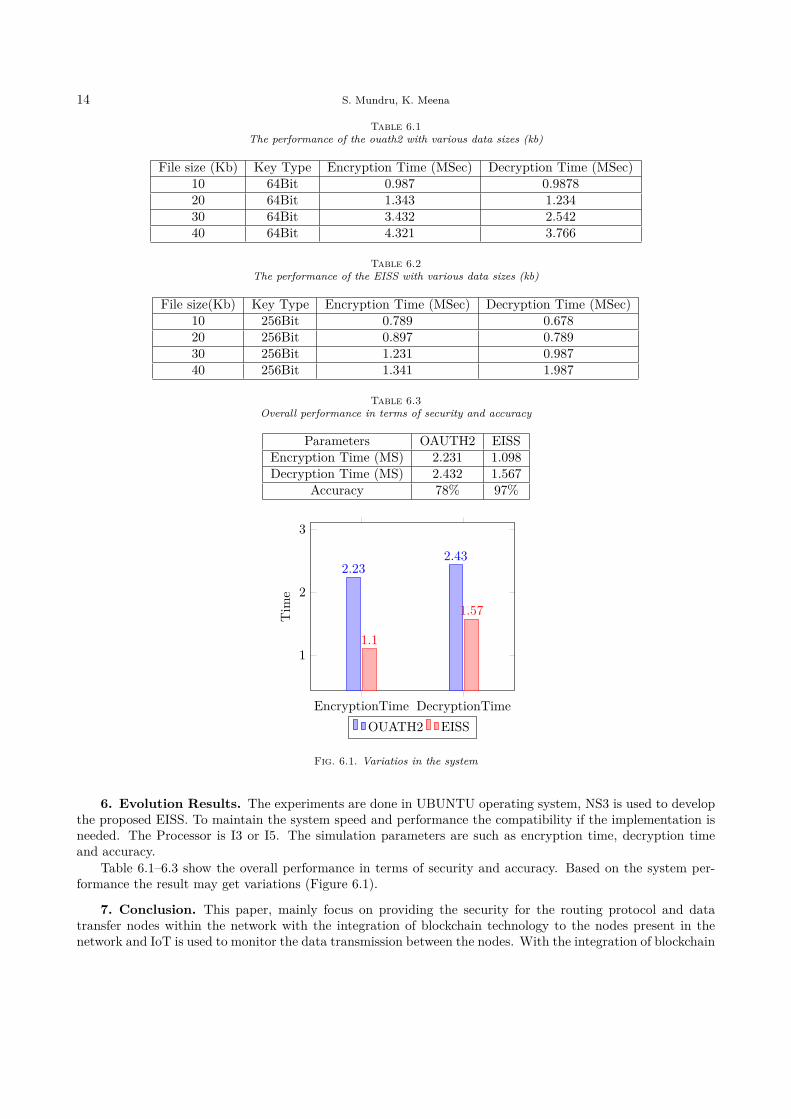
Table 6.1The performance of the ouath2 with various data sizes (kb)
File size (Kb) Key Type Encryption Time (MSec) Decryption Time (MSec)10 64Bit 0.987 0.987820 64Bit 1.343 1.23430 64Bit 3.432 2.54240 64Bit 4.321 3.766
Table 6.2The performance of the EISS with various data sizes (kb)
File size(Kb) Key Type Encryption Time (MSec) Decryption Time (MSec)10 256Bit 0.789 0.67820 256Bit 0.897 0.78930 256Bit 1.231 0.98740 256Bit 1.341 1.987
Table 6.3Overall performance in terms of security and accuracy
Parameters OAUTH2 EISSEncryption Time (MS) 2.231 1.098Decryption Time (MS) 2.432 1.567
Accuracy 78% 97%
EncryptionTime DecryptionTime
1
2
3
2.232.43
1.1
1.57Tim
e
OUATH2 EISS
Fig. 6.1. Variatios in the system
6. Evolution Results. The experiments are done in UBUNTU operating system, NS3 is used to developthe proposed EISS. To maintain the system speed and performance the compatibility if the implementation isneeded. The Processor is I3 or I5. The simulation parameters are such as encryption time, decryption timeand accuracy.
Table 6.1–6.3 show the overall performance in terms of security and accuracy. Based on the system per-formance the result may get variations (Figure 6.1).
7. Conclusion. This paper, mainly focus on providing the security for the routing protocol and datatransfer nodes within the network with the integration of blockchain technology to the nodes present in thenetwork and IoT is used to monitor the data transmission between the nodes. With the integration of blockchain

An Ensemble Integrated Security System with Cross Breed Algorithm 15
and IoT the security is provided very highly to transfer the data within the nodes. To access the data betweenthe nodes the private and public keys are generated with RSA algorithm. According to the EISS the threeparameters are calculated to improve the performance of the security and accuracy.
REFERENCES
[1] K. Ashton, That ‘Internet of Things’ in RFID J., Jun. 2009.[2] R. Minerva, A. Biru,and D. Rotondi, Towards a definition of the Internet of Things (IoT), IEEE Internet Initiative,
vol. 1, pp. 1-86, 2015.[3] A. Al-Fuqaha, M. Guizani, M. Mohammadi, M. Aledhari, and M. Ayyash, Internet of Things: A survey on enabling
technologies protocols and applications, IEEE Commun. Surveys Tuts., vol. 17, no. 4, pp. 2347-2376, 4th Quart. 2015.[4] Savelyev, LU-A. Copyright in the Blockchain era: Promises and challenges, Comput. Law Secur. Rev. 2018, 34, 550–561.[5] Kshetri, N, Blockchain’s roles in strengthening cybersecurity and protecting privacy,Telecommun. Policy 2017, 41, 1027–1038.[6] Kim, S.-K.; Huh, J.-H, A Study on the Improvement of Smart Grid Security Performance and Blockchain Smart Grid
Perspective. Energies 2018, 11, 1.[7] H. Suo, J. Wan, C. Zou, J. Liu, Security in the Internet of Things: A review, Proc. Int. Conf. Comput. Sci. Electron. Eng.
(ICCSEE), vol. 3, pp. 648-651, 2012.[8] C. Kolias, G. Kambourakis, A. Stavrou, J. Voas, DDoS in the IoT: Mirai and other Botnets, Computer, vol. 50, no. 7,
pp. 80-84, 2017.[9] S. Sicari, A. Rizzardi, C. Cappiello, D. Miorandi, A. Coen-Porisini, Toward data governance in the Internet of Things,
in New Advances in the Internet of Things, Cham, Switzerland:Springer, pp. 59-74, 2018.[10] M. U. Farooq, M. Waseem, A. Khairi, S. Mazhar, A critical analysis on the security concerns of Internet of Things
(IoT),Int. J. Comput. Appl., vol. 111, no. 7, pp. 1-6, 2015.[11] Y. Ai, M. Peng, and K. Zhang, Edge computing technologies for internet of things: a primer, Digital Communications and
Networks, vol. 4, no. 2, pp. 77–86, 2018.[12] A. Alrawais, A. Alhothaily, C. Hu, and X. Cheng, Fog computing for the internet of things: Security and privacy issues:
IEEE Internet Computing, vol. 21, no. 2, pp. 34–42, 2017.[13] R. Buyya and A. V. Dastjerdi, Internet of Things: Principles and paradigms, Elsevier, 2016.[14] Hopali, Egemen and Vayvay, Ozalp(2018). , Internet of Things (IoT) and its Challenges for Usability in Developing
Countries, IJIESR.1. 6-9
Edited by: Swaminathan JNReceived: Sep 7, 2019Accepted: Dec 9, 2019


Scalable Computing: Practice and Experience, ISSN 1895-1767, http://www.scpe.org© 2020 SCPE. Volume 21, Issue 1, pp. 17–31, DOI 10.12694:/scpe.v21i1.1603
BACKGROUND MODELLINGUSING A Q-TREE BASED FOREGROUND SEGMENTATION
SHAHIDHA BANU S ∗AND MAHESWARI N†
Abstract. Background modelling is an empirical part in the procedure of foreground mining of idle and moving objects. Theforeground object detection has become a challenging phenomenon due to intermittent objects, intensity variation, image artefactand dynamic background in the video analysis and video surveillance applications. In the video surveillances application, a largeamount of data is getting processed by everyday basis. Thus it needs an efficient background modelling technique which couldprocess those larger sets of data which promotes effective foreground detection. In this paper, we presented a renewed backgroundmodelling method for foreground segmentation. The main objective of the work is to perform the foreground extraction only inthe intended region of interest using proposed Q-Tree algorithm. At most all the present techniques consider their updates to thepixels of the entire frame which may result in inefficient foreground detection with a quick update to slow moving objects; Theproposed method contract these defect by extracting the foreground object by controlling the region of interest (the region onlywhere the background subtraction is to be performed) and thereby reducing the false positive and false negative. The extensiveexperimental results and the evaluation parameters of the proposed approach with the state of art method were compared againstthe most recent background subtraction approaches. Moreover, we use challenge change detection dataset and the efficiency of ourmethod is analyzed in different environmental conditions (indoor, outdoor) from the CDnet2014 dataset and additional real timevideos. The experimental results were satisfactorily verified the strengths and weakness of proposed method against the existingstate-of-the-art background modelling methods.
Key words: Background modelling, dynamic background, foreground detection, background subtraction, Quad Tree segmen-tation
AMS subject classifications. 68U10, 94A08
1. Introduction. The noteworthy increase in the number of cameras being used for the purpose of videoanalysis and surveillance is due to low cost of higher resolution cameras. However, some issues always holdback users related to the surveillance of the captured videos, for example the cost will be more as we maintainthe recorded data a long duration. Thus it is required for a motion detection algorithm which forms basicworking of background subtraction, which can further build a background model to which the current frame iscompared.
The background subtraction algorithm is therefore required to discriminate foreground from background.The static part of the scene here is background and the moving objects are the foreground. While a staticbackground model is enough to analyses short videos in a controlled indoor environment, it is insufficient formost practical cases; Therefore, a more refined model is required to handle dynamic background, backgroundwith shadow and illumination change. Moreover, the motion detection is on the preliminary step in any of theapplication related to surveillance. For example, finding the region where moving object is detected might bemade available for the further analysis or processing of unattended objects, ghost removal, human monitoring,traffic control, etc. Thus, background subtraction (BS) is the normal approach to detect motion in videos.The procedure is termed as foreground segmentation which involves frame comparison, update to backgroundmodel and foreground segmentation. This procedure produces a binary mask.
Background modeling [18, 19],is a process of considering the background under different condition. A goodalgorithm should correctly detect the moving object, and at the same time remove the shadow. Besides, it isalso important that it must exactly extract the foreground having same color as the background. A ”universal”background subtraction algorithm has to handle the following critical situations:
∗Research Scholar, SCSE, VIT University – Chennai Campus, Chennai-600127, India ([email protected])†Professor, SCSE, VIT University – Chennai Campus, Chennai-600127, India.
17

18 Shahidha Banu S, Maheswari S
• Noise in the image due to sudden and gradual lightning variation• Detecting slow moving object as well intermittent objects where the non-static object stays for a periodof time as the static object.• Movement of objects in the background as well multiple foreground objects.• Handling shadow region.
It is complicated to achieve these goals with a simple background subtraction, by design, that promotes atthe pixel level for improved productivity and it is not easy to analyze significant change patterns to producebetter results.
The BS algorithm performs the task in two stages: background modelling and foreground extraction.The modeling is all about the measured design of the background demonstration and a technique engaged toaccommodate the background changes at different timing instant. The object detection refers to the methodengaged for pixel classification; generally, it is a threshold process where the present value x of the active pixelis compared to the same pixel in the B(x) background model. Conferring to the calculated difference in pixelvalue, x may be classified as foreground when the calculated difference is greater than threshold and when it isrelatively smaller the pixel x is considered to be background. Furthermore, this procedure indirectly involvesa mechanism using feedback among the modeling and the foreground detection modules. It is also a criticalphase in reducing the misclassifications and increasing the accuracy in foreground segmentation. This probleminvades an open choice between various methods for updating the background pixels.
In this paper, we present an adaptive region based background modeling method for the efficient foregroundsegmentation. The proposed method detects the primary region into which background subtraction to beperformed. Region adjustments are regulated by monitoring: 1) moving objects in the background; 2) similaritybetween observed foreground and background models; 3) instable region based on regular fluctuations; and 4)the transmission of changing brightness or so called illumination changes. These four regulations are used asalgorithm framing guide for an efficient foreground segmentation technique. The rest of the paper is organized asfollows: In Section II, we comprehensively review the literature of background modeling techniques. This workgives an idea about the other frameworks developed for the purpose. Some of the methods are implementedand results are taken for comparison with our routine. Section III labels our method and specifies the routinesused in our major research work: the background model initialization process, finding the region of interest andthe update policy. Section IV deliberates the metric parameters used, and the experimental results along withcomparisons and execution performance.. We show that performing background subtraction in the specifiedregion alone in its simplified form is equivalent the other techniques that are more sophisticated. The conclusionis given in Section V.
2. Literature Review. Ample count of background modeling methods have been offered over the pastdecades to identify or to fragment the foreground objects in a video stream. They commonly follow the generalprocedure of considering the initaial frame or the mean of first few frames as background model, and thenit finds the pixel based difference between the the current frame with the background model to sense theforeground objects. Various proposed modeling methods either parametric or Non-parametric were categorizedinto pixel-based, region or block based, and hybrid. One of the popular parametric methods which is alsopixel-based is the Gaussian model. Wren et al. [1], which is considered to be first pixel based backgroundmodelling method.
However, a simple Gaussian function is not suitable to detect slow moving objects and frames with dynamicbackground due to lack of update mechanism to the background model [2]. Movements of tree leaves and waterwaves are considered to be dynamic background [3],and Stauffer and Grimson [4, 5] recommended a modelthat works on every pixel of the frame called the Gaussian mixture model (GMM). It is the procedure whichworks with mixture of K-mean Gaussians functions. As an improvement to above method, EM-based algorithmoffered where it introduces a way to initialize the factor through online in the modelling of background, whichis left to be time consuming. Adaptive Gaussian was proposed by Zivkovic,[30, 6] who anticipate an update tothe parameters and D.S.Lee [7] has proposed a mechanism to improve the combining rate without diturbingthe gaussian [5] stability as an adaptive learning rate. . Chien et al. [49] throws a threshold based factor forthe object detection. Here, they consider the camera noise and set to zero mean in gaussian distribution sinceit is the only factor that affects the threshold.

Background Modelling Using a Q-Tree Based Foreground Segmentation 19
Shimada et al. [8] introduces a varying component to control the GMM in order to increase the accuracyand to reduce the computational time. Also, Oliver et al. [10] introduced a background modelling methodbased on Bayesian method which uses the previous information of data and keeps gathering proof from thedataConsidering the Non-Parametric category in background modeling methods, Maddalena et al. [18] proposeda nonparametric algorithm based artificial neural networks with self-organization (SOBS). Kim et al. [19, 20]proposed a method of codebook which performs background modelling that initializes codeword and storesthe statitics of codeword used in the codebook. Barnich et al. [11, 12] projected a pixel-based algorithmfrom the category nonparametric named Vibe. It detects the moving object as foreground using a the patternof sampling intensity and random selection strategy. Wang et al.[42] suggested a technique (SACON) usingmanipulative sample consensus based on every pixel of the statistical model. The model detects the foregroundobject by exploiting both color and motion information. The superior performance to many other state-of-the-art methods is considered to be ViBe and is considered to be the exact method that detects the backgroundchanges in every frames [13]. The further study about the Vibe method was conceded by Droogenbroeck andPaquot [14] and they promote the performance enhancement by enhancing the ViBe with some consideredadditional constraints. Another such pixel based non parametric method proposed by Hofmann et al. [15] ispixel based adaptive segmenter (PBAS) method. The method keeps track of history of recent time observedpixel values and these are applied as background model to segment the foreground object. Although, the resultof above discussed state-of-art methods projects well the outlines of foreground objects,i.e. the shape of theobject and Also, they are affected by various factors like noise, dynamic background and lighting changes ,etcwithout any difficulty.
As an another approach to Pixel-based background modelling there exist theRegion-based methods.It usesthe inter-pixel relations to enhance its efficiency and segments the images into regions and performs foregroundobjects identification from the segmented image regions. Kernel Estimation Density(KDE) projected by El-gammal et al. [9, 28] offered a novel method by building a nonparametric background model. Seki et al. [50]applied a different technique of background modelling by applying image variation co-occurrence in the definedimage regions. A heuristic algorithm distinguishes the foreground object from the background based on blockmatching and similar method was proposed by Russell et al. [51] to . In which they compared fixed size ofbackground regions with the input frames. In order to provide solution to the dynamic background modelingchallenges in outdoor settings, Eng et al. [52] offered a random regular arrangements and image regions withpre filters, by using color space to detect foregrounds in the ClELab. Furthermore the method is featured bycolor and texture based analysis which receives a attractive attention among region based methods.An anotherbackground modelling method proposed by Heikkila et al. [53] engaged a technique called local binary pattern(LBP) , which involves the discriminative texture feature of the image for modeling the background.In theabove model, LBP histogram is built for partially overlapping regions and the same will be compared againstthe LBP histogram of every incoming frames regions. Liu et al. [54] proposed a method to resolve the challengeof illumination change. It is also an efficient background modeling method for foreground segmentation basedon binary descriptor and proven to adapt under continuously varying illumination condition. In addition, an-other method based on binary descriptors was proposed by Huang et al. [55] as a sample based backgroundmodelling a replacement to parametric methods. In divergence to pixel-based foreground segmentation meth-ods,these region-based segmentation methods can obtain only coarse shapes of foreground objects but canreduce the misclassification to a greater extent, thus reducing the false correlations .
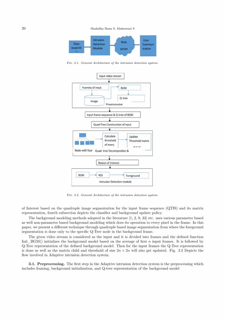
3. Proposed Architecture for Q-tree based Intrusion Detection System. Here we have proposedan architecture for an Intrusion detection and prevention system. The Fig. 4.1 portrays the flow in thearchitecture. The flow includes the data acquisition from the camera attached in the surveillance area isthen forwarded to the intrusion detection module which incorporate the proposed Q-Tree based foregroundsegmentation. Once the intrusion is detected in the surveillance area the intimation will be given to theprovided webserver which further gets forwarded to the user by the webserver.
The data acquisition model collects the video data from the camera in the area under surveillance regionand is given to the IDM(Intrusion detection model) which in turn incorporates our proposed approach usingthe concept of ”Q-tree Image segmentation(QIS) ”. In first subsection, we presented preprocessing technique,second subsection explains the Q-Tree Decomposition, third subsection focuses on the routine to find Region
20 Shahidha Banu S, Maheswari S
Fig. 3.1. General Architecture of the intrusion detection system.
Fig. 3.2. General Architecture of the intrusion detection system.
of Interest based on the quadruple image segmentation for the input frame sequence (QTIS) and its matrixrepresentation, fourth subsection depicts the classifier and background update policy.
The background modeling methods adopted in the literature [1, 2, 9, 33] etc. uses various parameter basedas well non-parameter based background modeling which does its operation to every pixel in the frame. In thispaper, we present a different technique through quadruple based image segmentation from where the foregroundsegmentation is done only to the specific Q-Tree node in the background frame.
The given video stream is considered as the input and it is divided into frames and the defined functionInit_BGM() initializes the background model based on the average of first n input frames. It is followed byQ-Tree representation of the defined background model. Then for the input frames the Q-Tree representationis done as well as the matrix child and threshold of size 2n × 2n will also get updated. Fig. 3.2 Depicts theflow involved in Adaptive intrusion detection system.
3.1. Preprocessing. The first step in the Adaptive intrusion detection system is the preprocessing whichincludes framing, background initialization, and Q-tree representation of the background model

Background Modelling Using a Q-Tree Based Foreground Segmentation 21
Fig. 3.3. (a) The background frame; (b) Q-Tree based image segmentation; (c) Tree representation segmented image.
1. FramingThe video stream is considered as the input and is divided into the frames suitable for further processingand is stored in the local database for the foreground identification and Intrusion detection.
2. Background InitializationIt is the first step but considered to be an important step in the process of background subtraction.There are various well know methods available to model the initial background. Few such is assigningthe average illumination of first n frames, or assigning the very first frame directly as BGM, or usingthe image order to approximate the background model, and the frame average over the time. Althoughthe average of background frame that updates at an instance of time tn is familiar with many systems,it is not good enough to handle shadow and ghost problems. Here, we adopt a modest and proficientway of initializing the background where the median of first n frames are considered. When consideringthe median of first n frames, It also reflects the illumination change. At the initial time t0, we set theinitial background as the median of first n frames.
Init_BGM =Median(fk)
where k varies from 1, 2, . . . , n at the timing instance t0. The initial background plays a vital role in theprocess since the foreground detection that happens at timing instance tj depends on the backgroundframe detected at t0, where j is closer to n.
3. Q-Tree representation of the Background modelThe initial frame which is set as the background model is taken and is given with the Q-Tree representa-tion. The background image is divided into regions with varying information. This is accomplished bythe Q-Tree decomposition technique. Such decomposition is powerful as it gives homogeneous regionswhich in further gets constructed as a tree with each parent having maximum of four children. Eachchild corresponds to a quadrant of the segmented image frame as shown in Fig. 3.3.The tree representation is also given with a coding procedure where 1 is given for the node with a childi.e. if node is a parent and 0 for child node which do not further have a child. So for the above tree inFig. 3.3(c) , the Q-Tree code(QTC) is given as 1-0000.
3.2. Q-Tree Decomposition and its Representation. Assuming the size of image array is m × n,the entire image array is represented by quadruple tree. The Q-tree will have four child representing the fourquadrants of the array and each of the child will be subdivided in a recursive manner. The procedure terminatesthe Q-Tree with leaves with homogeneous regions or until the specified level. These leaves correspond to theunique regions of the image segments.
Here the root of the tree corresponds to the entire image. When Q-tree iteration takes place at the firstiteration, the image is segmented into four quadrants. Thus, resulting the tree with four homogeneous leaves.The iterations can be further continued until desired level or desired pixels are segmented. A sustainablecondition is set by finding the pixel intensity difference and must be lesser than the threshold. The differencebetween high intensity pixel and low intensity pixel is calculated within the node of the decomposed quad treeand is ensured against the sustainability condition. Each level in the decomposed tree is given with 2n × 2nnodes for the given integer n, where n corresponds to the number of iterations. For example, at 0 split thewhole image is represented as the singe node. At 1st split the image is segmented into 21 × 21 nodes whichrepresents the four quadrants of the parent image frame.
Each node has left and right segments denoted by l, r, and top, bottom segments denoted by t, b, respectively.So each image is denoted by four disjoint set as nodes and are represented by tl, tr, bl, br in the clockwise order.

22 Shahidha Banu S, Maheswari S
Also for n splits, the total number of nodes in the tree is given by formula,No. of nodes in the tree = 4n−1
3
Since the scope of the research work is restricted to intrusion detection, we limit the value of n to 2.So thatmaximum of two levels are possible and the level 0,1,2 corresponds to whole image, image with 4 quadrantsand image with 16 regions respectively.
Q-Tree decomposition is performed by considering the input image frame of size m ×n. At each iteration,it divides the image frame into four quadrants and assign it as four children to the parent node. The same getsiterated for every child node until desired pixels are selected. At each iteration it updates the array QTC andQTT which corresponds to Q-Tree code and Q-Tree node threshold, respectively.
QTCi[2m][2n] =
{1 for parent node0 for child node
for all 0 ≤ m ≤ 2, 0 ≤ n ≤ 2. (3.1)
QTTi[2m][2n] = {adaptive threshold of the specific node} , for 1 ≤ m ≤ 2m, 1 ≤ n ≤ 2n. (3.2)
In the above equation QTCi is the array which holds vale 1 for parent node and 0 for child node. Thus QTC0
holds 0 since there is no splitting, QTC1 holds 4 values in a two dimensional array [21], QTC2 holds 16 valuesas it corresponds to [22], 4× 4 matrix array. Similarly QTTi corresponds to the respective adaptive thresholdof the node. QTCi has been given with a third value 2 when every pixel in the region is a foreground pixel.The algorithm for Q-Tree decomposition is as follows.
Algorithm: Q-Tree DecompositionInput: Input FramesOutput: Q-Tree segmented image frame with QTC and QTTStep 1: Ensure I is the Image frameStep 2: Check whether the dimension of I is m× nStep 3: Perform the Quad tree decomposition of IStep 4: Update the array QTC and QTT , for every iteration i according eqs (3.1) and (3.2)Step 5: Calculate the pixel intensity Pi as follows
Pi(x, y) =14
∑1m=0
∑1n=0 xi − 1(2x+m, 2y + n)
Step 6: for m,n = 0, 1, 2 if Pi−1(2x+m, 2y + n) are leaves go to step 5Step 7: Check equation in 5-6 for sustainability condition
|Pi(x, y)− Pi−1(2x+m, 2y + n)| < TIf true, set as leafOtherwise set as node
Step 8:continue step 5 for next x,yEnd procedure
3.3. Finding ROI In Background Model. Most of the state of art background modeling methodskeep only single background frame for foreground segmentation, in which the result of foreground detectionconsumes the whole frame. This procedure is termed as FBM ( frame-based background modeling). Theinadequacy of the background modeling process opens a large room for the scholars to post their ideas. Manytimes the background modelling faces a problem where the part of the generated background may be inaccuratebecause of the problems like slow moving objects, image ghost and the shadows. The next problem is that theaccuracy of background update may get worse as the frame distance increases, most cases this varies with framecompression rate. To solve these complications, we come out with a region- based background model (RBM).The enhancements that are noticed with the proposed method are at spatial level where foreground generationand segmentation mechanism performed on the basis of ROI but not entire frame. The other improvement is,in temporal level, where background generation and modeling are performed for every frame but not a wholevideo sequence.
Some of the literature discussed are the block based methods like Heikkila et.al.[71] proposed a methodthat models the scattering of block texture in a frame using the local binary pixel outline method. Moreover, in

Background Modelling Using a Q-Tree Based Foreground Segmentation 23
these block-based methods [71, 72, 73] there is a recurring problem of dealing with the entire frame. Althoughthey consider the frame as a gathering of blocks, they perform their operation to entire block segments andreassemble those blocks back to frames.
To avoid these problems, we offered an algorithm to find the region of interest in the background to whichthe foreground segmentation is constrained. This approach presents two main ideas where it works on a Q-Treeof the background model. QTC is the code given for the regions in the image segments. For the point P onthe frame f , the coordinates are given as Pi,j and the point P on the background is given as Bi,j and the pixelintensity difference is given as Di,j . When there is the change in intensity i.e. |Di,j | ̸= 0, then it is classified asforeground pixel. On the other hand, If there is no change in the intensity where |Di,j | = 0, then QTC code isset as follows.
Procedure: Find_ROI()Input : Q-tree of frame f in the video streamOutput : Segmented foreground.Algorithm:Step 1: Read QTCi[2m][2n], QTTi[2
m][2n];Step 2: check for QTCi[2m][2n]; for i = 0, 1, 2;Step 3: If code=0, the region has no intrusion;
Not a ROIClassify every pixel in the region as background pixel;
Step 4: If code=1, the region has some intrusion;Is a ROICollect coordinates within the region and calculate change in IntensityDi,j = |Pi,j −Bi,j |if |Di,j | ̸= 0 then
classify as foreground,else
classify as background;end if
Step 5: Goto step 2 for the next i;End procedure
The above procedure is used to check for the intensity change which corresponds to the foreground appear-ance, illumination change and many other issues.
3.4. Foreground Segmentation And Background Update. Once the ROI is determined, the nextstep is to perform the foreground segmentation. The colossal of the existing method includes ViBe, PBAS,Word consensus model. The ViBe set the first frame as background and foreground segmentation is done usingthe fixed threshold. This restriction holds back the adaptability of the method. PBAS, the non-parametricbackground model integrates the ideas of state-of-art foreground detection methods and works in a controlledenvironment. Here we follow the basic idea of ViBe, PBAS with some variations to provide an efficient segmen-tation. Fixed threshold of ViBe is replaced by an adaptive threshold, and the first frame as background modelis over laced by the median of first n frames. To update the background model, we use the adjustable learningrate concept from the PBAS with a random scheme and dynamic threshold is used to identify the foreground.The algorithm has two important factors: T (x), L(x) which corresponds to the dynamic threshold and learningrate for background update The background model Bi(x) for the pixel x is defined as B(x).
B(x) = {B1(x), · · · , Bk(x), · · ·Bn(x)} , where 1 < k < n
Pixel x is considered to be the foreground pixel when the given condition holds true
f(x) =
{1 if dist((Ix), (Bx)) < T (x)0 otherwise (3.3)

24 Shahidha Banu S, Maheswari S
The above formula illustrates that f(x) is set to 1, i.e. the pixel is classified as foreground, when thedistance between the current frame and the background frame is lesser than the dynamic threshold. Otherwise,set with 0 means the pixel x is the background pixel.
The dynamic threshold changes its value at each frame over the time instance tn, for nth frame. It iscalculated by the formula as suggested in the literature [74].
∆T = α1
w · h
n−1∑i=0
|I(x)−B(x)| (3.4)
Since it changes with time, it is considered to be dynamic and the pixel we use the notation delta T, α isthe coefficient called inhibitory coefficient, whose reference value is 2. w · h represents the width and height ofthe frame which in turn represents the size of the frame. The algorithmic representation is given below.
Algorithm: Pixel classificationInput : Input frame, ROIBOutput: Classified Foreground objectProcedure:for zi ϵ ROIB for every row in the ROI
for zi ϵ 1, 2, · · ·w for every pixel in the row docalculate difference between the pixel at background frame (at time t− 1) and current frame (at time t).calculate Dist(Bt−1(xy), It(xy));
end forDt(x) = minyϵ0, 1, 2, · · · , w − 1Dist(Bt−1(xy), It(xy))Distance at time instance tUpdate T (x) using the equation (3.4)Classify the pixelIf Dt(xy) < T (xy) then
F (xy) = 1;Else
F (xy) = 0;End if
End forEnd procedure.
The above procedure is used to perform the background subtraction only to the region of interest predictedin the previous step. The procedure is repeated for every line in the ROI and for every pixel x of the line thedistance is calculated, then compared with dynamic threshold, QTTi[2m][2n]. If the intensity difference is lesserthan the threshold then it is classified as foreground otherwise classified as background.
As proposed in ViBe, the update mechanism used is the conservative type where it never includes the pixelto the background which belongs to the foreground. Thereby, avoids the misclassification and keeps the falsepositive minimum.
4. Experiemental Analysis. Hereby, we discuss the quantitative and qualitative performance evaluationof the proposed technique. For which we presented the foreground segmentated image as qualitative evaluation.Then, parameter based metrics evaluation compared with the results of five other recent state-of-art techniques.
4.1. Evaluation metrics and the Test Dataset. The video sequences of the Change Detection Chal-lenge 2014 dataset [75] has been used to assess the execution performance of the proposed approach both as aqualitative and quantitative evaluation . Since it is confirmed in many of the works, it is clear that traditionaldatasets are cramped and lacks challenging video streams. Moreover, standard methods have outperformedand no longer face the challenges of current video surveillances application.
The Change Detection Challenge 2014 dataset has been promised with 53 videos of 11 categories includingthe states of both outdoor as well indoor videos. These videos have been prearranged under categories Base-

Background Modelling Using a Q-Tree Based Foreground Segmentation 25
line, dynamic background, camera jitter, Intermittent object motion, shadows, thermal signatures, challengingweather, low frame-rate, night videos, PTZ capture and air turbulence. The baseline is considered to be animportant category that includes the following challenges: background motion, isolated shadows, having un-controlled objects and ghost. The intermittent object motion is the category that has the video with movingobject stays static for some time and again started to move. To measure the accuracy, we calculated few metricsnamely F-measure, percentage of correctness.
Classification (PCC) and Matthew’s correlation coefficient (MCC) metrics are referred in the literaturesF-Measure[SOIR], PCC[word consensus model], MCC and are calculated using terms true positive (TP), truenegative (TN), false positive (FP), false negative (FN). To calculate the metrics it is assumed like foregroundas positive and background as negative. When it is correctly detected then true, otherwise it is false. Thus,True positive is the number of pixels where foreground pixels are correctly detected as the foreground, falsepositive depicts the number of background pixels wrongly detected as the foreground, True negative representsbackground pixels correctly detected as the background and False negative represents the number of foregroundpixels wrongly detected as background. These metrics in turn are used to calculate precision and recall.
Precision is the foreground prediction which is measured as the ratio of correctly classified foreground pixelsto the total number of pixels classified as foreground pixels which include the misclassification.
Precision =TP
TP + FP(4.1)
The precision is calculated since it gives the ability of the method to identify foreground pixels (consideringmisclassified positive class). The Recall measures the detection rate and is calculated as the ratio of correctlyclassified foreground pixels to the total number of foreground pixels in the ground truth (i.e. ratio of truepositives to actual foreground pixels in the test image).
Recall =TP
TP + FN(4.2)
The above two metrics namely precision and Recall are used in calculating the evaluation metrics likeF-measure, PCC, MCC which are used to assess the quality of a method; As just, the method is considered ifit has high Recall values, without losing Precision. F-Measure is the metric obtained as the weighted harmonicaverage of the values recall and precision. It is the metric used in most of the datasets to rank the methods. Itis defined as follows:
FMeasure = 2 · Recall · PrecisionRecall + Precision
(4.3)
The metric percentage of correct classification (PCC) is also used to determine whether both the backgroundand foreground is classified correctly. For an effective foreground segmentation, PCC value must hold high.The PCC value is calculated using the below given equation:
PCC =TP + TN
TP + TN + FP + FN(4.4)
The last metric used for evaluating the performance is Matthew’s Correlation Coefficient(MCC) scores. Asstated in the literature [2], it is found to assess the overall performance of unbalanced binary classification, intowhich the background subtraction comes in. it is calculated using the formula
MCC =(TP ∗ TN)− (FP ∗ FN)√
(TP + FP ) ∗ (TP + FN) ∗ (TN + FP ) ∗ (TN + FN)(4.5)
4.2. Results of challenge change detection 2014 dataset.. We compared our method to six otherrecent foreground segmentation methods, the adaptive background modeling(ABMFS)[78], the word consen-sus model(PAWCS) [77], the Gaussian mixture model (GMM) [6], the sample consensus background model(SACON) [17], ViBe [76], the pixel-based adaptive segmentation (PBAS) [79], the boosted Gaussian model
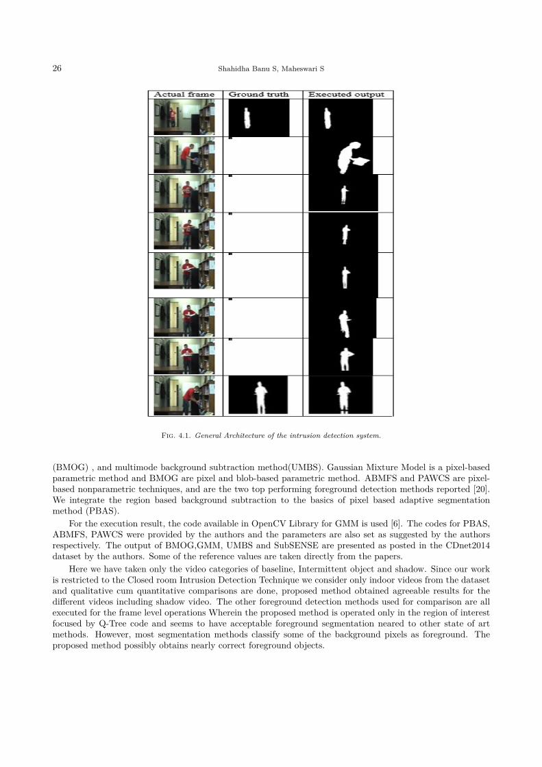
26 Shahidha Banu S, Maheswari S
Fig. 4.1. General Architecture of the intrusion detection system.
(BMOG) , and multimode background subtraction method(UMBS). Gaussian Mixture Model is a pixel-basedparametric method and BMOG are pixel and blob-based parametric method. ABMFS and PAWCS are pixel-based nonparametric techniques, and are the two top performing foreground detection methods reported [20].We integrate the region based background subtraction to the basics of pixel based adaptive segmentationmethod (PBAS).
For the execution result, the code available in OpenCV Library for GMM is used [6]. The codes for PBAS,ABMFS, PAWCS were provided by the authors and the parameters are also set as suggested by the authorsrespectively. The output of BMOG,GMM, UMBS and SubSENSE are presented as posted in the CDnet2014dataset by the authors. Some of the reference values are taken directly from the papers.
Here we have taken only the video categories of baseline, Intermittent object and shadow. Since our workis restricted to the Closed room Intrusion Detection Technique we consider only indoor videos from the datasetand qualitative cum quantitative comparisons are done, proposed method obtained agreeable results for thedifferent videos including shadow video. The other foreground detection methods used for comparison are allexecuted for the frame level operations Wherein the proposed method is operated only in the region of interestfocused by Q-Tree code and seems to have acceptable foreground segmentation neared to other state of artmethods. However, most segmentation methods classify some of the background pixels as foreground. Theproposed method possibly obtains nearly correct foreground objects.

Background Modelling Using a Q-Tree Based Foreground Segmentation 27
Table 4.1Average quantitative values of evaluation metrics from change detection dataset
Scenarios Percentage of Recall Precision F-measurecorrectnessclassification
Bad Weather 98.5 0.604 0.315 0.411Baseline 96.0 0.901 0.849 0.874Camera Jitter 93.8 0.791 0.359 0.495Dynamic Background 99.1 0.655 0.200 0.317Intermittent motion object 97.5 0.815 0.835 0.824Low frame 89.7 0.640 0.645 0.642Night Video 92.0 0.802 0.502 0.616PTZ 84.5 0.725 0.287 0.410Shadow 96.8 0.914 0.503 0.649Thermal 98.5 0.865 0.623 0.727Turbulence 97.4 0.710 0.559 0.625Overall 94.9 0.763 0.516 0.615
Another quantitative comparative approach on experimental result on the Change Detection Challengedataset is presented were we broadly test the proposed method. Here, the scenario considered includes Baseline,Intermittent motion objects, and Shadows. The other category usage is suppressed due to the scope of theresearch.
The qualitative analysis is given above with representation of actual frame, its ground truth and theexecuted output. Table 4.1 depicts the average values of the metrics Recall, Precision, F-measure and percentageof correctness classification. It projects the average value from the CDnet14 dataset for all the categories ofvideos in the open dataset. These average metric values are used for comparison of the proposed algorithm.Though at some places the proposed algorithm can not achieve remarkable enhancement, it goes above theaverage from the dataset.
Table 4.2 presents evaluation metrics F-Measure score of different video criteria considered for our methodin comparison with six other high performing methods on the CDnet 2014 dataset. The values of top threeperforming methods are given in red, blue and yellow color shade. Though our method performed best only forthe videos pedestrian and copy machine, it is clearly visible that the performance of other criteria office, parking,bus station is also evaluated to very near of well performed methods The proposed modeling method couldacclimate to speedy changes caused by slow background changes, as well to illumination variation and staticobjects since it can execute more number of frames per second. Though, the performance is not good for thecategory sofa, the overall scores proven to be the best performance. For the same the graphical representationis given in Fig.4.
Table 4.3 also shows in detail the PCC metric values in the compared state of specific criteria Baseline,Intermittent motion object and Shadows respectively. It could be proven that our method obtained higherscores in every criteria at least for one video frame sequences. The top three values are represented with boldred, blue and yellow respectively. Table 4.4. Also represent the MCC( Mathew’s Correlation Coefficient) withits graphical representation in Fig.4.3
5. Conclusion and Future Work. In this paper, we proposed an adaptive and efficient backgroundmodeling technique that exploits region based background subtraction. It also provides quick response tothe real time scenario with data inconsistency. Furthermore, we have introduced “Q-Tree based foregroundsegmentation” algorithm to model the background that selects the specific region in a faster manner andpromotes efficient foreground segmentation. This selection mechanism works well in most situations withvarying conditions. The experimental result shows that the overall performance of proposed method is betterthan the entire benchmark systems considered. The method was proposed to identify the moving object in theregion of interest, and to perform pixel based background subtraction for foreground detection. Satisfactorily,

28 Shahidha Banu S, Maheswari S
Table 4.2Comparitive F-Measure values of the selected methods from CDnet14
Method / Video Baseline Intermittent object Shadow
Category Pedestrian Office Parking Sofa CopyMachine Bus Station
proposed 0.981 0.959 0.768 0.734 0.940 0.891ABMFS 0.957 0.972 0.618 0.846 0.871 0.869PAWCS 0.946 0.937 0.819 0.725 0.914 0.973GMM 0.960 0.656 0.482 0.652 0.660 0.787BMOG 0.920 0.626 0.698 0.632 0.640 0.823SUBSENSE 0.954 0.963 0.4447 0.742 0.929 0.864UMMBS 0.938 0.965 0.672 0.769 0.807 0.677
Table 4.3Comparative PCC values of the selected methods from CDnet144
Method / Video Baseline Intermittent object Shadow
Category Pedestrian Office Parking Sofa CopyMachine Bus Station
proposed 99.962 99.433 97.932 97.934 99.160 99.022ABMFS 99.916 99.616 94.507 98.747 98.239 98.995PAWCS 99.892 99.166 97.323 98.075 98.869 99.051GMM 99.919 96.332 95.603 97.608 96.113 98.584BMOG 99.833 95.510 96.168 97.222 95.729 98.770SUBSENSE 99.912 99.491 94.456 98.115 99.047 98.945UMMBS 99.871 99.517 95.335 98.216 97.675 98.174
proposed method performed the task of foreground segmentation in the identified region of interest with areduced mis-classification which results in better scores for the metrics considered. Thus, the quantitativeperformance is achieved. However, method shows lack in performance for the criteria shadow elimination,Baseline of CDnet2014.We will attempt to solve these issues using adaptive threshold for specific region basedon the learning rate to the specific region.
6. Acknowledgement. We thank the team who made the website (www.changedetection.net) availableand for providing the resource to test and compare our method.
REFERENCES
[1] C. Wren, A. Azarhayejani, T. Darrell, A.P. Pentland, IEEE Trans. PatternAnal. Mach Intell. 19 (7) (1997) 780-785.[2] M. Piccardi, IEEE Int. Conf. Syst. Man Cybern 4 (Oct. 2004)3099-3104. The Hague, The Netherlands.[3] Y. Benezeth, P.M. Jodoin, B. Emile, H. Laurent, C. Rosenberge, Review and evaluation of commonly-implemented
background subtraction al- gorithms, in: Proc. IEEE Int. Conf. Pattern Recognit, Dec.2008, pp. 1-4.[4] C. Stauffer, E. Grimson, Adaptive background mixture models for real-time tracking, in: Proc. IEEE Int. Conf. Comput.
Vis. Pattern Recog- nit., vol. 2, 1999, pp. 246-252.[5] C. Stauffer, E. Grimson, IEEE Trans. Pattern Anal. Mach. Intell. 22 (8)(Aug. 2000) 747-757.[6] Z. Zivkovic, Improved adaptive Gaussian mixture model for background subtraction, in: Proc. 17th Int. Conf. Pattern
Recognit., vol. 2, Aug. 2004, pp. 28-31.[7] D.S. Lee, Pattern Anal Mach. Intell. IEEE Trans. 27 (5) (May 2005)827-832.[8] A. Shimada, D. Arita, R.I. Taniguchi, Dynamic control of adaptive mixture-of-Gaussians background model, in: AVSS
’06 Proceedings ofthe IEEE International Conference on Video and Signal Based Surveil- lance, IEEE Computer SocietyWashington, DC, USA, 2006.
[9] A. Elgammal, D. Hanvood, L.S. Davis, Non-parametric model for background subtraction, in: Proc. ECCV 2000, June2000, pp. 751e767.
[10] N.M. Oliver, B. Rosario, A.P. Pentland, IEEE Trans. Pattern Anal. Mach.Zntell. 22 (8) (2000) 831-843.

Background Modelling Using a Q-Tree Based Foreground Segmentation 29
Table 4.4Comparative MCC values of the selected methods from CDnet14
Method / Video Baseline Intermittent object Shadow
Category Pedestrian Office Parking Sofa CopyMachine Bus Station
proposed 0.981 0.956 0.857 0.747 0.936 0.887ABMFS 0.956 0.970 0.591 0.842 0.862 0.865PAWCS 0.946 0.934 0.806 0.740 0.910 0.868GMM 0.960 0.672 0.459 0.667 0.657 0.785BMOG 0.921 0.611 0.698 0.626 0.628 0.818SUBSENSE 0.954 0.960 0.516 0.7487 0.924 0.860UMMBS 0.938 0.962 0.650 0.767 0.805 0.704
Fig. 4.2. Graphical representation of PCC
Fig. 4.3. Graphical representation of MCC.

30 Shahidha Banu S, Maheswari S
[11] O. Barnich, M. Van Droogenbroeck, Vibe: a powerful random technique to estimate the background in video sequences,in: IEEE Int. Conf. on Acoustics, Speech and Signal Processing, 2009, pp. 945e948.
[12] O. Barnich, M. Van Droogenbroeck, IEEE Transaction Image Process. 20 (6) (2011) 1709-1724.[13] Y. Min-Hsiang, H. Chun-Rong, L. Wan-Chen, L. Shu-Zhe, C. Kun-Ta, IEEE Transaction Cirt.s Syst. Video Technol. 25
(4) (2015) 595-608.[14] M. Van Droogenbroeck, O. Paquot, Background subtraction: experiments and improvements for ViBe, in: Proc. IEEE
Comput. Soc. Conf. Comput. Vis. Ptrn Recognit. Workshops, Jun. 2012, pp. 32-37.[15] M. Hofmann, P. Tiefenbacher, G. Rigoll, Background segmentation with feedback: the pixel-based adaptive segmenter,
in: Proc. IEEE Comput. Soc. Conf. Comput. Vis. Pattern Recognit. Workshops, Jun. 2012, pp.38-43.[16] K. Kim, T. Chalidabhongse, D. Harwood, L. Davis, Background modeling and subtraction by codebook construction, in:
Int. Conf. on Image Processing, 2004, pp. 3061-3064.[17] K. Kim, T. Chalidabhongse, D. Harwood, L. Davis, Real-Time Imaging 11 (3) (2005) 172-185.[18] L. Maddalena, A. Petrosino, IEEE Transaction Image Process. 17 (7) (2008) 1168-1177.[19] Y. Benezeth, P.M. Jodoin, B. Emile, H. Laurent, C. Rosenberge, J. Electron Imaging (July 23, 2010).[20] A. McIvor, Background subtraction techniques, in: Proc. Image Vis .Comput., Auckland, New Zealand, Nov. 2000.[21] R. Radke, S. Andra, O. Al-Kofahi, B. Roysam, IEEE Transaction on Image Process 14 (Mar. 2005) 294-307.[22] S. Elhabian, K. El-Sayed, S. Ahmed, Recent Pattern. comput. Sci. 1 (Jan.2008) 32-54.[23] T. Bouwmans, F. El Baf, B. Vachon, Statistical background modeling for foreground detection: a survey, in: Handbook
of Pattern Recogn. and Computer Vision, vol. 4, World Scientific, Singapore, Jan. 2010, pp. 181-199 ch. 3.[24] S. Panahi, S. Sheikhi, S. Hadadan, N. Gheissari, Evaluation of back- ground subtraction methods, in: Proc. Int. Conf. on
Digital Image Computing: Techniques and Applications, IEEE, Piscataway, NJ, 2008, pp. 357-364.[25] D. Parks, S. Fels, Evaluation of background subtraction algorithms with post-processing, in: Proc. of IEEE Int. Conf. on
Advanced Video and Signal Based Surveillance, 2008, pp. 192-199.[26] A. Sobral, BGSLibrary: an opencv cþþ background subtraction library, in: IX Workshop de Viso Computa-
cional (WVC’2013). Rio de Janeiro, Brazil, 2013. Software available at: http://code.google.com/p/bgslibrary/. [39]http://www.changedetection.net.
[27] A. Mittal, N. Paragios, Motion-based background subtraction using adap- tive kernel density estimation, in: Proc. Int.Conf. On Computer Vision and Pattern Recognition, IEEE, Piscataway, NJ, 2004, pp. 302-309.
[28] A. Elgammal, R. Duraiswami, D. Harwood, L. Davis, Proc. IEEE 90 (7) (Jul. 2002) 1151-1163.[29] Y. Sheikh, M. Shah, IEEE Trans. Pattern Anal. Mach. Intell. 27 (11) (Nov. 2005) 1778-1792.[30] Z. Zivkovic, F. van der Heijden, Pattern Recognit. Lett. 27 (May 2006)773-780.[31] A. Tavakkoli, M. Nicolescu, G. Bebis, M. Nicolescu, Mach. Vis. Appl. 20 (Oct. 2008) 395-409.[32] C. Ianasi, V. Gui, C. Toma, D. Pescaru, Facta Univ. Ser. Elec. Energ. 18 (1) (Apr. 2005) 127-144.[33] A. Tavakkoli, M. Nicolescu, G. Bebis, An adaptive recursive learning technique for robust foreground object detection,
in: ECCV 2006, May 2006.[34] A. Tavakkoli, M. Nicolescu, G. Bebis, Robust recursive learning for foreground region detection in videos with quasi-
stationary backgrounds, in: ICPR 2006, Aug. 2006.[35] A. Tavakkoli, M. Nicolescu, G. Bebis, Automatic statistical object detection for visual surveillance, in: IEEE Southwest
Symposium on Image Analysis and Interpretation, Denver, Colorado, SSIAI 2006, March 2006.[36] T. Tanaka, A. Shimada, D. Arita, R. Taniguchi, Non-parametric back- ground and shadow modeling for object detection,
in: ACCV 2007, Nov.2007, pp. 159-168.[37] R. Ramezani, P. Angelov, X. Zhou, A fast approach to novelty detection in video streams using recursive density estimation,
in: International IEEE Symposium on Intelligent Systems, vol. 2, Sept. 2008, pp. 142e147.[38] T. Kohonen, Learning vector quantization, Neural Networks vol. 1, 1988, pp. 3-16.[39] B.D. Ripley, Pattern Recognition and Neural Networks, CambridgeUniversity Press, 1996.[40] A. Ilyas, M. Scuturici, S. Miguet, Real time foreground-background segmentation using a modified codebook model, in:
Advanced Video and Signal Based Surveillance, 2009.[41] Z. Zivkovic, F. van der Heijden, IEEE Trans. PAMI 26 (5) (2004). [55] Pattern Recognit. (2007) 1091-1105.[42] H. Wang, D. Suter, Background Subtraction Based on a Robust Consensus Method, Proceedings of the 18th International
Conference on Pattern Recognition (ICPR’06), pp. 223-226.[43] L. Maddalena, A. Petrosino, The SOBS algorithm: what are the limits ?, in: CVPRW 2012, June 2012, pp. 21-26.[44] K.E.A. Sande, T. Gevers, C.G.M. Snoek, IEEE Trans. Pattern Anal.Mach. Intell. 32 (9) (Sep. 2010) 1582-1596.[45] P.-M. Jodoin, M. Mignotte, J. Konrad, IEEE Trans. Circuits Syst. Video Technol. 17 (12) (Dec. 2007) 1758-1763.[46] T. Bouwmans, F. El Baf, B. Vachon, Recent Pat. Comput. Sci. 1 (3) (2008) 219-237.[47] R. Cucchiara, M. Piccardi, A. Prati, IEEE Trans. Pattern Anal. Mach.Intell. 25 (10) (Oct. 2003) 1-6.[48] E.L. Hall, Computer Image Processing and Recognition, Academic Press, 1979.[49] S.-Y. Chien, W.-K. Chan, Y.-H. Tseng, H.-Y. Chen, IEEE Trans. Circuits Syst. Video Technol. 23 (6) (Jun. 2013) 921-934.[50] M. Seki, T. Wada, H. Fujiwara, K. Sumi, Background subtraction based on cooccurrence of image variations, in: Proc.
IEEE Comput. Soc. Conf. Comput. Vis. Pattern Recognit, Jun. 2003, pp. II-65eII-72.[51] D. Russell, S. Gong, A highly efficient block-based dynamic background model, in: Proc. IEEE Conf. Adv. Video Signal
Based Surveill, Sep.2005, pp. 417-422.[52] H.-L. Eng, J. Wang, A.H.K.S. Wah, W.-Y. Yau, IEEE Trans. Image Process. 15 (6) (Jun. 2006) 1583-1600.[53] M. Heikkil€a, M. Pietik€ainen, IEEE Trans. Pattern Anal. Mach. Intell. 28 (4) (Apr. 2006) 657-662.[54] W.-C. Liu, S.-Z. Lin, M.-H. Yang, C.-R. Huang, Real-time binary descriptor based background modeling, in: Proc. IAPR
Asian Conf. Pattern Recognit, Nov. 2013, pp. 722-726.
Background Modelling Using a Q-Tree Based Foreground Segmentation 31
[55] G.-H. Huang, C.-R. Huang, Binary invariant cross color descriptor usinggalaxy sampling, in: Proc. 21st Int. Conf. PatternRecognit, Nov. 2012, pp. 2610-2613.
[56] Y. Nonaka, A. Shimada, H. Nagahara, R. Taniguchi, Evaluation report of integrated background modeling based onspatio-temporal features, in: Proc. IEEE Comput. Soc. Conf. Comput. Vis. Pattern Recognit. Work- shops, Jun. 2012,pp. 9-14.
[57] S.-S. Huang, L.-C. Fu, P.-Y. Hsiao, IEEE Trans. Circuits Syst. VideoTechnol. 19 (4) (Apr. 2009) 522-532.[58] T.H. Tsai, C.-Y. Lin, S.-Y. Li, IEEE Trans. Circuits Syst. Video Technol.23 (1) (Jan. 2013) 15-e29.[59] A. Schick, M. Bauml, R. Stiefelhagen, Improving foreground segmen- tations with probabilistic superpixel Markov random
fields, in: Proc. IEEE Comput. Soc. Conf. Comput. Vis. Pattern Recognit. Workshops, Jun. 2012, pp. 27-31.[60] Y.-T. Chen, C.-S. Chen, C.-R. Huang, Y.-P. Hung, Pattern Recognit. 40 (10) (Oct. 2007) 2706-2715.[61] M. Cristani, M. Bicego, V. Murino, Integrated region- and pixel-based approach to background modeling, in: Proc.
Workshop Motion Video Comput, Dec. 2002, pp. 3-8.[62] Y. Wang, P.-M. Jodoin, F. Porikli, J. Konrad, Y. Benezeth, P. Ishwar, Cdnet 2014: an expanded change detection
benchmark dataset, in: Computer Vision and Pattern Recognition Workshops (CVPRW), 2014 IEEE Conference on.IEEE, 2014, pp. 393-400.
[63] T. Ojala, M. Pietikainen, T. Maenpaa, IEEE Trans. Pattern Anal. Mach.Intell. 24 (7) (Jul. 2002) 971-987.[64] Z. Zivkovic and F. van der Heijden, “Efficient adaptive density estima tion per image pixel for the task of background
subtraction,” Pattern Recognit. Lett., vol. 27, no. 7, pp. 773–780, 2006.[65] N. Goyette, P.-M. Jodoin, F. Porikli, J. Konrad, and P. Ishwar, “Changedetection.net: A new change detection
benchmark dataset,” in Proc. IEEE Comput. Soc. Conf. CVPRW, Jun. 2012, pp. 1–8.[66] P. Kaew, Tra Kul Pong and R. Bowden, “An improved adaptive background mixture model for real-time tracking with
shadow detection,” in Video- Based Surveillance Systems. New York, NY, USA: Springer, 2002, pp. 135–144.[67] J. Guo, C. Hsia, Y. Liu, M. Shih, C. Chang, and J. Wu, “Fast background subtraction based on a multilayer codebook
model for moving object detection,” IEEE Trans. Circuits Syst. Video Technol., vol. 23, no. 10, pp. 1809–1821, Oct. 2013.[68] T. S. F. Haines and T. Xiang, “Background subtraction with Dirichlet process mixture models,” IEEE Trans. Pattern Anal.
Mach. Intell., vol. 36, no. 4, pp. 670–683, Apr. 2014.[69] K. Kim, T. H. Chalidabhongse, D. Harwood, and L. Davis, “Real-time foreground-background segmentation using
codebook model,” Real- Time Imag., vol. 11, no. 3, pp. 172–185, Jun. 2005.[70] Eli Shusterman,”Image compression via improved quadtree decomposition algorithm”,IEEE Trans. On Image Process-
ing,Vol.3,No.2,March 1994.[71] Heikkila, M., and Pietikainen, M., ‘A texture-based method for modelling the background and detecting moving objects’,
IEEE Trans.Pattern Anal. Mach. Intell., 2006, 28, pp. 657–662.[72] Tian, G., and Men, A., ‘An improved texture-based method for background subtraction using local binary patterns’. Image
and Signal Processing, (CISP), Tiajin, China, 2009.[73] Liao, S., Zhao, G., Kellokumpu, V., Pietikainen, M., and Li, S., ‘Modelling pixel process with scale invariant local
patterns for background subtraction in complex scenes’. IEEE Conf. on Computer Vision and Pattern Recognition,(CVPR), San Francisco, CA, USA, 2010
[74] R.S.Rakibe, Prof.B.D.Patil, “Human motion detection using background subtraction algorithm,” Int. Journal of Advanceresearch in CS and SE., vol. 4, no. 2, pp. 45-48, Feb. 2014.
[75] N. Goyette, P. M. Jodoin, F. Porikli, J. Konrad, and P. Ishwar, “Changede- tection.net: A new change detectionbenchmark dataset,” in Proc. IEEE Conf. Comput. Vis. Pattern Recognit. Workshops, Jun. 2012, pp. 1–8.
[76] O. Barnich and M. Van Droogenbroeck, “ViBe: A universal background subtraction algorithm for video sequences,”IEEE Trans. Image Process., vol. 20, no. 6, pp. 1709–1724, Jun. 2011.
[77] Pierre-Luc St-Charles, Guillaume-Alexandre Bilodeau, and Robert Bergevin, “Universal Background SubtractionUsing Word Consensus Models,” IEEE Trans.on image processing, vol. 25, no.10, pp. 747–757, Oct. 2016.
[78] Zuofeng Zhong, Bob Zhang, Guangming Lu, Yong Zhao, and Yong Xu, “An Adaptive background modeling methodfor foreground segmentation,” IEEE Trans. Intell. Transp. Syst., vol. 18, no. 5, pp. 1109-1120, May 2017.
[79] A. Sobral and A. Vacavant, “A comprehensive review of background subtraction algorithms evaluated with synthetic andreal videos,” Comput. Vis. Image Understand., vol. 14, pp. 4–21, May 2014.
[80] Ma, M., Hu, R., Chen, S., Xiao, J., & Wang, Z.,” Robust background subtraction method via low-rank and structuredsparse decomposition”. China Communications, 15(7), 156–167, July 2018.
[81] Roy, K., Arefin, M. R., Makhmudkhujaev, F., Chae, O., & Kim, J. “ Background Subtraction Using Dominant DirectionalPattern”. IEEE Access, 6, 39917–39926, December 2018.
[82] Mingliang chen,Zing wei,Qingxiong yang,Qing Li,Gang Wang, Ming-Hsuan yang, “Spatiotemporal GMM for Back-ground Subtraction with superpixel Hierarchy,” IEEE Trans. Pattern Anal. Mach. Intell., vol. 40, no.6, pp. 1518- 1526,June 2018.
Edited by: Swaminathan JNReceived: Sep 12, 2019Accepted: Dec 9, 2019


Scalable Computing: Practice and Experience, ISSN 1895-1767, http://www.scpe.org© 2020 SCPE. Volume 21, Issue 1, pp. 33–40, DOI 10.12694:/scpe.v21i1.1607
TOPOLOGICAL ORDERING SIGNAL SELECTION TECHNIQUE FOR INTERNET OFTHINGS BASED DEVICES USING COMBINATIONAL GATE FOR VISIBILITY
ENHANCEMENTAGALYA RAJENDRAN∗AND MUTHAIAH RAJAPPA†
Abstract. In modern System on Chip (SoC) design consist of intelligence of products, Internet of Things (IoT) based devices,mobile phones, laptops, servers etc. This shrinking market reduces the design automation validation process. Signal selection isthe most effective and challenging technique in post-silicon validation and debug. The vital problem prevailing in this method isthat it has limited observability and controllability due to the minimum number of storage space in the trace buffer. This tends toselect the signals prudently in order to maximize the state reconstruction. To identify the trace signals, signal restoration is theextensive metric that has been used so far. Topology-based restoration method is proposed here to minimize the error detectionlatency which helps to select the trace signals with minimum error or even errorless. This method aid to detect more number oferrors within limited number of clock cyclesthan the restoration only selection techniques.
Key words: Design bugs, Error detection, Internet of Things (IoT), Restorability, Topology, Trace signal, validation
AMS subject classifications. 94A12
1. Introduction. Recent System-on-Chip (SoC) design studies specifies the extensive usage of SoCs in theelectronic industry with increasing complexity in design circuits and its influence to meet the demands in evergrowing technologies from various applications containing Internet of Things (IoT). Since there is a growing inthe technology it is difficult to meet the functional correctness of the circuits during pre-silicon validation. Theescaped errors (both functional and electrical errors) must be captured during posts-silicon validation. Fig. 1.1represents the key components in the design industry.
The main challenge in post-silicon validation (psv) is that it has limited observability and controllabilityof internal signals after the first silicon is available [1]. Because of poor observability of internal signals, it isvery difficult to debug the design and electrical errors in this atmosphere is laborious [2, 3]. Electronic designautomation (EDA) tools are used to automate the product development cycle and validation to achieve theanticipated results with minimum cost and time that ensures the efficiency. Controllability defines the ability ofmoving an internal signals from input to output. On-chip buffers are used to control these signals.Compare toseveral methods, scan chain is the most effective technique to enhance both the observability and controllabilityof internal signal states for the determination of manufacturing. However, it is very less effective during chipexecution of debugging and validation [4]. At that time of verification, it need to halt the process to readoutthe each state of flip-flops.Few signal states are stored in the trace buffer within a limitedno.of clock cycles byincorporating it to the on-chipto attain the non-destructive state of internal signals. Only small set of signalscan be traced due to the constraint of area overhead. There is a difficulty in the selection of correct signals sincethey are selected at the design stage. For smaller deign circuit, it is easy to recommend few signals based onthe designers own knowledge but for larger design circuit like automated signal selection, it is difficult. Hence,restoration of signals helps to increase the visibility of untraced signals from the value of traced flip-flops [5].This is the most common method for finding the signals automatically. From [6, 7, 8, 9], none of the papershas discussed about the effectiveness of detecting or localizing the errors.
∗Research scholar, School of Computing, SASTRA Deemed University, Thanjavur, Tamilnadu. India. ([email protected]).
†Associate Dean, School of Computing, SASTRA Deemed University, Thanjavur, Tamilnadu. India ([email protected]).
The authors sincerely thank DST-INSPIRE Fellowship and SASTRA Deemed University for providing a great support.
33

34 Agalya Rajendran, Muthaiah Rajappa
Fig. 1.1. Interconnected market propellers
This paper is focusing on the efficacy of bugs and latency that present in the traced signals that may affectobservability and controllability enhancements. These effects can be observed at the gate-level selection. Analternative way is proposed at this level of selection that considers a path along the traced gates and theirtopological sort rather than considering flip-flops only. By this way, it reduces the error detection latency andincreases the erroneous responses from the traced gates.
The remaining paper is organized by research background and how this work motivates us are described inSection II. In Section III and IV, the authors proposed the signal section techniques and their findings basedon the topological sorting respectively. In section V they have conclude their research work.
2. Research Backgroundand Motivation.2.1. Background. The state restoration (SRR) can be done either by forward restoration or backward
restoration of unknown signal states that are traced during silicon debug [1]. This helps to decide which signalare to be traced in an automatic manner to increase the rate of post- silicon validation part. It can be definedas
SRR =Number of states restored + traced signals
Number of states traced (2.1)
The visibility of internal signals increases if the state restoration value increases. It may be helpful to findthe root cause of internal design bugs when debugging. There is a wide variety of selection techniques wereexisted and it may cause a serious issue while debugging. One such factor is that assuming all the signals arehaving equal importance in the selection process and it is really unrealistic from the point of debugging. But inreality, which internal signals are ought tobe observed that varies between design structure and design feature.Existing methods like [10], attempted to link the trace signal selection method with debugging, error detectionand localization. But their methods were not appropriate to find the location of random errors. If few flip-flopsare traced, it can affect the other flip-flop when the bit flip is detected if they consider different restorationscenarios [12]. However in [11], they critically analyzed about the state restoration but they strongly suggestthe usage of assertion coverage to sort out the trace signal problems. This method is restricted to one type oferror model and their signal selection methodology is commendable for missing error models.So there is lackin standardizing the error models in psv is the biggest weakness for the evaluation of various signal selectionalgorithms and deign bugs are categorized from few of reported works [13]. Some bugs were missed out at thegate level abstraction like exchange of wires, inverters, etc. This is the starting point to propose this paperby taking the above said bugs as our motivating example. The bugs in the RTL, translated into gate levelmanifestations. In our experiment we consider different instances to represent a single design bug.

Topological ordering Signal Selection Technique for Internet of Things based Devices using Combinational Gate 35
Fig. 2.1. Example circuit from [4,5]
2.2. Motivation. To elucidate the irrelevances between the actual error localization and the signal selec-tion algorithms, we simulated the gate-level description of Fig. 2.1 [6]. For example, here we are simulating2 different types of errors. Primarily, haphazard gate replacement is consider as type 1 bugs and exchange ofwires between the circuit is consider as type 2 bugs. As we know that some bugs are not identifiable at thepre-silicon stage under some circumstances. For example, if the design has two input Ex-OR gate that can bereplaced by two input OR gate but the only identification of replacement of the gate is ’11’. This is the placewhere we can fails to identify the state at pre-silicon stage when the corresponding state is activated rarely inthe state machine. Similarly, type 2 bugs are also justified in this section.
A quick identification of a bug location is observed and its latency report is shown in table 2.1 and 2.2 basedon gate replacement before Flip-flop ’C’ and exchange of wires between flip-flops ’C’ and ’F’ respectively. Here,we experiment 4 number of iterations by injecting an error. ’NO’ represents either the error doesn’t propagatethrough the flip-flop or cannot be observed (Not observed). In paper [6], they consider AC and AB and in [5, 9]they consider C&F are the combination to achieve high restoration. If SRR helps to find out the erroneousresponse then these combinations can capture all kind of errors as soon as possible. But in the above tableit is evident that the gates which helps to get high SRR value will not observe the errors at all times. If twosignals gives high restoration value but if one is traced and the other is restored fully then it will be ineffectivefor error identification. Because tracing of one correlated signal is ineffective then the restored states were also
Table 2.1Type 1 bug latency (Gate replacement)
Errors FlipflopsA B C D E F G H
Error1 NO NO NO 1 1 2 3 3Error2 NO NO 1 3 2 3 4 4Error3 NO NO 1 2 3 3 4 4Error4 NO NO 2 3 4 4 1 5Error5 NO NO 2 4 3 4 1 5Error6 NO NO NO NO NO NO NO NO
Table 2.2Type 2 bug latency (Exchange of wires)
Errors FlipflopsA B C D E F G H
Error1 NO NO 1 2 NO 2 3 4Error2 NO NO 1 NO 2 2 3 4Error3 NO NO NO NO NO 1 2 2Error4 NO NO 1 3 NO NO 2 NOError5 NO NO 1 NO 3 NO 2 NOError6 NO NO 1 NO 3 NO NO 2Error7 NO NO 1 3 NO NO NO 2

36 Agalya Rajendran, Muthaiah Rajappa
Table 2.3Buggy restored states of Fig. 2.1
Clock cycles/ Flip-flops A B C D E F G HCycle1 0 0 1 0 0 0 ND NDCycle2 0 0 1 1 0 0 0 0Cycle3 0 0 1 0 0 0 0 0Cycle4 0 0 1 0 0 0 0 0Cycle5 ND ND 0 0 0 0 0 0Cycle6 ND ND 0 0 0 0 0 0Cycle7 0 0 1 0 0 0 0 0Cycle8 0 0 1 0 0 0 0 0
follows the same tendency.As mentioned earlier, restoration is the only criteria that fails to address the debug and validation in an
appropriate manner. In [9], some of the restored sates does not illustrate for the erroneous design. Sometimesthese are different from the actual state that demonstrates in Fig. 2.1 Type 1 bugs are performed to introducethe design bugs. If the trace buffer width is 2, then C and F are the selected to trace the signal combinationsin [5]. Here Table 2.3 shows the buggy design of eight restored states of flip-flops. The highlighted positionindicates the conflict value of actual response of design bugs. This is done for 8 cycles, at least one of valuesof each cycle have the conflict values instead of actual restoration value. This is point we consider to proposethis system with the following points since it is undesirable for circuit misbehavior in comparison to actualresponse. One is the multiple occurrences of false restoration which can affect the root cause of the problemand can increase the debug time. And the second is, the incorrect values may lead to wrong path when try tolocalizing the error during backtracing.
3. Proposed Method. To improve the signal observability, restoration plays a major role since theuntraced signals are restored from the traced signal states. In these approaches, flip-flops are not consideredfor error propagation whereas it is purely depends on the presence and absence of combinational paths in thecircuit between the flip-flops (internal signals). So we adventure this principle in our proposed methodology byallowing circuit topology.
At first, we create an S-graph to examine the error propagation from one gate to the other since the actualbugs are present on the combinational path is the main issue. However the reported work says it is a tediousprocess hence they have used flip-flops instead of gates present on the path. Therefore the proposed workconcentrates on the error propagation through the gates using topological sort is the main concept to reducethe complexity. So that it reduces the time and identifies the errors that propagates through the combinationalpath. While creating an S-graph, gates are represented as nodes and the flip-flops between the gates arerepresented as path with directed weighted edges. To optimize the error detection and latency, we are orderingthe gates in design structure (Algorithm 1). The traced signals must capture the bugs/errors within limitednumber of clock cycles, so that this method can ensure the error detection latency is curtailed.
It is not necessary to trace the neighborhood of primary output, it can be done at the primary outputwith high latency. The vicinity of primary input (PI) can be ignored from a set of traced signals that canobserve erroneous behavior through flip-flops. After performing the topological sort (S-graph), the list of gatesare pruned until the elements are compared with the width of the trace buffer. The main intension behind theabove sorting is to select the gate that can capture higher number of erroneous behavior as early as possible.But this method has major limitation that the topological order can be done only on acyclic graph but thereal circuits have more number of cycles. Because of this reasons, group of gates forming cycles into singleregion and then it becomes a directed acyclic graph. This definitely causes implications on bug propagation inorder to bug detection. Hence, this aids to give rudimentary solution incurred by limited topological order. Anode in a graph (SG) has definite no.of inputs and outputs. The weights are calculated between the edges oftwo gates along the path. SG’’ indicates the conversion of building SG by grouping the nodes as acyclic graphwhich forms a cycles into a single node. For larger cycles this conversion of SG’’ can break the cycle. To selectthe particular node we need to find out which node has more priority that gives higher visibility. The outlineof the procedure is given in Algorithm 2.

Topological ordering Signal Selection Technique for Internet of Things based Devices using Combinational Gate 37
Table 3.1Algorithm 1
1. Create S-graph (Input: Design; Output: Graph (SG))Total_gates (G)= count the total no.of gates2. for each gate Gi doGatesremaining = Gatestotal −Gi
3. for each gate Gj in Gremaining donode← 0;4. if path exists between Gj to Gi thennode← node+ 1; end ifend for5. edge weight =node6. node← 0;7. link Gi and Gj using edge weight8. end for9. SG’=directed weight of the design graph10. SG =Convert SG”
Table 3.2Algorithm 2
1. Priority node allocation (Input: Graph (SG); Output: priority list)2. For each node Ni of graph do3. Edgeinput = no.of incoming edges of each node4. Edgeoutput = no.of outgoing edges of each node5. Weightinput = incoming edge weight6. Weightoutput = outgoing edge weight7. Notch = Edgeinput ( Σ Weightinput ) + Edgeoutput (Σ Weightoutput)8. List = priority of each node9. end for
Table 3.3Algorithm 3
1. Find pruning_factor pf ( Input: Graph (SG), Trace_buffer bandwidth (TB),list of priority node values; Output : Pruning factor)2. Graph_list = Topological order (SG)3. Temp_list = Graph_list4. Pruning_factor= first_pf5. While Temp_list > TB do6. Temp_list’ = pruned factor of Temp_list7. Total_priority node values = � Temp_list’8. Number = no.of Temp_list’ entries9. Avg_value = Tot_priority node values/ number10. Store pruning_factor and avg_score in a list11. Pf = pf+pf_increment12. Temp_list = Temp_list’13. end while14. pf = pf of highest avg_score
The node values are calculated and it assigns the priority to each gates for the persistence of ranking withregards to error collection. These are calculated using how many number of connections are there from one flip-flop to the other. By multiplying the number of incoming and outgoing edges with their corresponding weightsare summed up to known the total number of connections present. After sorting of gates in the topologicalorder these should be cut down from the both the ends of primary input and primary output. The pruningfactor can be find by using Algorithm 3.
Here pruning factor (pf) signifies the node which are detached from the list of S-graph. It plays a major rolefor the selection of trace signal. The proposed fine-grained algorithm find out the optimal solution that beginswith complete topological order depends on first_pf and pf_increament. The remaining list is representedas Temp_list’, the priority node value calculation has done for the Temp_list’ and avg_score that obtained

38 Agalya Rajendran, Muthaiah Rajappa
Table 3.4Algorithm 4
1. Trace_SS (Input: Graph_list, pf, list of priority nodal values,TB_Bandwidth; Output: FF_list)2. Node value = value of each node from the priority list3. Graph_list’ = graph_list based on pf4. FF_list’ = sort graph_list by corresponding node value5. FF_list = FF_list’ entries based on TB_Bandwidth
Fig. 3.1. Directed Acyclic Graph (DAG)
during calculation. Here pf incrimination is based on the both pf and pf_increment. At last, highest value ofpruning factor of avg_score has chosen as pf. These are all based on the window size (ω) of the trace buffer.Based on the percentage of the size of the window, the topological order and the priority list; the arrangementswere done and it is shown in Algorithm 4. For example, the pruning factor of 80% and 60% are 0.1 and 0.2respectively. There is no pruning value for 100%. The topological sorting should be done before pruning factorfindings. With the help of both priority assignment and pruning factor, this proposed technique can find morenumber of bugs within limited clock cycles. To select the signals, the signal selection are done based on thetopological order. The remaining nodes of pruning order are arranged using priority node values. Based on thewidth of the trace buffer the signal selections are done with highest node value.
Based on the above four algorithms (table 3.1-3.4), the erroneous response can be find out easily. Considera design having 8-combinational gates and its directed acyclic graph is shown in Fig.3.1. This graph contains8-nodes and its reported results are shown in this section. Based on the priority, the node values are assignedand its corresponding edge values from G1 to G8 are 16, 4, 12, 9, 3, 32, 11 and 14 respectively. These valuesare arranged in decreasing order to compute the procedure. The pruning factor decides at the previous step isrepresented as the highest node value after detachment of gates at both the ends. Gate values and its orderingare represented below:
Gates(G1−G8)→ 1, 2, 3, 4, 5, 6, 7, 8V alues→ 16, 4, 12, 9, 3, 32, 11, 14
Table 3.5Topological order (TO) based on priority of node values
Window size (%) TO By its priority nodevalue (descending order)
100 1, 3, 7, 2, 4, 5, 6, 8 6, 1, 8, 3, 7, 4, 2, 580 1, 3, 7, 2, 4, 5, 60 1, 8, 3, 7, 4, 2, 560 3, 7, 2, 4, 5 1, 3, 7, 4, 5
Employing the distributed trace buffer concept rather than using a single trace buffer that helps to debugthe modules efficiently. This method can be applied to any larger circuit. For better understanding the authorshas taken the ISCAS ’89 benchmark circuit to represent it.

Topological ordering Signal Selection Technique for Internet of Things based Devices using Combinational Gate 39
4. Experimental Results. To evaluate the trace signal selection, some parameters should be identify.They are: State Restorability (SR), Error Detection Latency (EDL) and Non-Detected Bugs after injecting(NDB). The restoration principle can be applied to any type of signal selection like [5, 6, 7, 8]. However,these techniques were insufficient to increase the visibility of internal signal states than the proposed system.To estimate the weakened state of restoration, the above mentioned parameters are used to derive from thefollowing equation.
△ SR = SR {SRR based Trace _ SS} − SR {obtained Trace_ SS} (4.1)
△ EDL = EDL {SRR based Trace _ SS} − EDL {obtained Trace_ SS} (4.2)
△NDB = NDB {SRR based Trace _ SS} − NDB {obtained Trace_ SS} (4.3)
To evaluate the diminished states, the above mentioned parameters are used. △SR shows the differencebetween state restorations for the selected set of trace signals. The difference of error detection latency andthe number of errors are reported by △EDL and △BND. These three parameters are evaluated more thanthousand times on type 1 bug by injecting an error. The signals are selected using either by restoration methodor by our proposed topological method. Table 4.1 shows the evaluation of larger benchmark circuits of ISCAS’89using different parameters as follows. Since the restoration and error restoration approach incompetent, theprinciple operation of state restoration is applied on the above mentioned parameters.
Table 4.1Evaluation of proposed system with the bandwidth size of 16
Benchmark t No.of FFO SR EDL NDBCircuits38584 1426 0.906 3.86 152s38417 1636 -0.263 5.28 491s35932 1728 -0.01 39.4 223
There is an alternative method to find out the efficacy of trace signal selection using this proposed techniqueusing different bandwidth of trace buffer. These can be calculated using combinational score value by summingthe EDL and NDB for different window sizes (ω). The negative sign indicates that this method has higherrestorability than existing methods.
A (wi) = EDLi/EDL′i +NDBi/NDB
′i (4.4)
These can be applied to various modules of [6, 9]. To search the highest value the pruning factor shouldbe searched iteratively. It helps to find out the optimal solution from the pruning factor. As mentioned inprevious section, it is applicable to distributed modules. If the flip-flop of window size (ω) is traced, then theproposed system can detect the errors in limited cycles. It can be normalized with the help of pruning factorwith different window size. The proposed topological sorting method can be applied to automatically generatevarious learning paths for the mapping analysis concept.
Fig.4.1 shows the error detection ration between the three larger benchmark circuits. The error detectionis defined by
Error detection ratio =No. detected errorsNo. errors detectable (4.5)
Consider the circuit is divided into different regions and each region has one error-prone and we haveintroduced 50 random errors to the active regions and the error density is directly proportional to region size.Here, we executed two kinds of simulation one with an ideal case and the other with the erroneous signals. Wehave pragmatic our algorithm to various active regions.

40 Agalya Rajendran, Muthaiah Rajappa
Fig. 4.1. Comparison of error detection ratio for single active region
5. Conclusion. Trace buffers are used to store the traced value and to find out the root cause of errorsduring post-silicon validation and debug. State restoration technique fails to find out the errors present in thetraced signals whereas the proposed technique identifies the useful signals that can detect errors. To avoid theproblem of false restoration, we can consider the region-separation method. So that we can ensure the selectionof signals regardless of topological order.
Acknowledgement. The authors sincerely thank DST-INSPIRE Fellowship and SASTRA Deemed Uni-versity for providing a great support.
REFERENCES
[1] R. Agalya, and S. Saravanan, Recent trends on Post-Silicon validation and debug: An overview, International Conferenceon Networks & Advances in Computational Technologies (NetACT).,2017.
[2] J. Keshava, N. Hakim, and C. Prudi , Post-silicon validation challenges: How EDA and Academia can help, ACM/IEEEDesign Automation Conference (DAC), (2010), pp. 3-7.
[3] J. Goodenough, and R. Aitken , Post-Silicon Is Too Late Avoiding the $50 Million Paperweight Starts with ValidatedDesigns, ACM/IEEE Design Automation Conference (DAC), (2010), pp. 8-11.
[4] M. Abramovici, P. Bradley, K. Dwarakanath, P. Levin, G. Memmi, and D. Miller, reconfigurable design-for-debuginfrastructure for socs, 43rd ACM/IEEE Design Automation Conference, (2006), pp. 7–12.
[5] H. F. Ko and N. Nicolici, Algorithms for state restoration and trace signal selection for data acquisition in silicon debug,IEEE Transactions on Computer-Aided Design of Integrated Circuits and Systems., 28, (2009), pp. 285–297.
[6] K. Rahmani, P. Mishra, and S. Ray, Efficient trace signal selection using augmentation and ilp techniques, FifteenthInternational Symposium on Quality Electronic Design, (2014), pp. 148–155.
[7] K. Basu and P. Mishra, Rats: Restoration-aware trace signal selection for post-silicon validation, IEEE Transactions onVery Large Scale Integration (VLSI) Systems., 21, (2013), pp. 605–613.
[8] M. Li and A. Davoodi, A hybrid approach for fast and accurate trace signal selection for post-silicon debug, Design,Automation Test in Europe Conference Exhibition (DATE), (2013), pp. 485–490.
[9] X. Liu and Q. Xu, On signal selection for visibility enhancement in trace-based post-silicon validation, IEEE Transactionson Computer-Aided Design of Integrated Circuits and Systems., 31, (2012), pp. 1263–1274.
[10] K. Basu, P. Mishra, P. Patra, A. Nahir, and A. Adir, Dynamic selection of trace signals for post-silicon debug, 14thInternational Workshop on Microprocessor Test and Verification, (2013), pp. 62–67.
[11] S. Ma, D. Pal, R. Jiang, S. Ray, and S. Vasudevan, Can’t see the forest for the trees: State restoration’s limitationsin post-silicon trace signal selection, 2015 IEEE/ACM International Conference on Computer- Aided Design (ICCAD),(2015), pp. 1–8.
[12] A. Vali and N. Nicolici, Bit-flip detection-driven selection of trace signals, 221th IEEE European Test Symposium (ETS),(2016), pp. 1–6.
[13] D. V. Campenhout, T. Mudge, and J. P. Hayes, Collection and analysis of microprocessor design errors, IEEE DesignTest of Computers., 17, (2000), pp. 51–60.
Edited by: Swaminathan JNReceived: Sep 24, 2019Accepted: Oct 30, 2019

Scalable Computing: Practice and Experience, ISSN 1895-1767, http://www.scpe.org© 2020 SCPE. Volume 21, Issue 1, pp. 41–46, DOI 10.12694:/scpe.v21i1.1608
SECURED IDENTITY BASED CRYPTOSYSTEM APPROACH FOR INTELLIGENTROUTING PROTOCOL IN VANET
A KARTHIKEYAN ∗, P G KUPPUSAMY†, AND IRAJ S AMIRI* ‡
Abstract. Vehicular specially appointed systems named as Vehicular Ad-hoc NETwork (VANET) have been raising dependenton the condition of-art advancements in remote and system communication. The message confirmations among vehicles andinfrastructure are fundamental for the VANET security. The genuine personality of vehicles ought not to be uncovered, yetwhich is just detectable by approved nodes. Existing arrangements either depend vigorously on a carefully designed hardwareor cannot fulfill the security necessity. Secured Identity Based Cryptosystem Approach (SIDBC) for intelligent routing protocolis proposed for better results since implementing a secured network for traffic forecasting and efficient routing in dynamicallychanging environment. Polynomial key generation is utilized for generating identity based pseudonym keys for each and every nodethat comes under the system. This keying process protects the node from malignant node from passing false information. Theassessment output demonstrates that the planned method is more effective than past schemes since it is free pairing and it fulfillssecurity and protection prerequisites.
Key words: Data rate, Vehicular Ad hoc Networks, Trust Authority, Message Authentication, Polynomial Keys.
AMS subject classifications. 68M15
1. Introduction. VANET can be described in simple manner i.e. the vehicles that moves in the roadwaysare interconnected virtually by passing messages among them. It acts as a kind of Mobile Ad-hoc Networks(MANET) that comprises of mobile nodes and operates in a decentralized way. Infrastructure condition inwhich, moving devices can be in connection continuously. It is fundamentally formed by those elements thatdeal with the traffic or offer an outside administration. On one hand, producers are once in a while consideredinside the VANET model. A few unique functions are rising in VANETs that incorporates well-being relatedapplications to make more secured driving, portable business and other data benefits that will illuminate driversabout any kind regarding clog, driving perils, mishaps, roads turned traffic jams.
The paper organised is as follows section describes a formal introduction of VANET, section 2 depictsoverview of VANET, section 3 describes the proposed security identity based algorithm, section 4 deals withthe result analysis of the proposed and existing mechanism and section 5 provides the conclusion of this proposedmethodology.
2. Related Works. IVC comes under the operating system of VANETs which turn out to be admired incurrent years [1]. The vehicles function here as mobile nodes and they are connected together wirelessly. Theprinciple contrast is that versatile switches which manufacture the system are vehicles like cars or trucks. Manyacademic communities are working for enabling new applications with respect to VANETs [2, 3] for reducingroad hazards. Significant role of the method is to enhance the road safety measures.
Several safeties related approaches have been undertaken in VANET environments to enable secure infor-mation transmission among vehicles. Identity aware system that has main impacts in reducing accidents andincreasing traffic control services were discussed, here the information is shared among them in a timely manner.Public Key Algorithms (PKA) was proposed [4, 5, 6] for providing safety measurements during information
∗Associate Professor, Department of Electronics and Communication Engineering, Vel Tech Multi Tech Dr.RangarajanDr.Sakunthala Engineering College, Avadi, Chennai, India. ([email protected])
†Professor, Department of Electronics and Communication Engineering, Siddharth Institute of Engineering & Technology,Puttur, Andhra Pradesh, India, ([email protected])
‡Computational Optics Research Group, Advanced Institute of Materials Science, Ton Duc Thang University, Ho Chi Minh City,Vietnam. Faculty of Applied Sciences, Ton Duc Thang University, Ho Chi Minh City, Vietnam. ([email protected])
41

42 A. Karthikeyan, P.G. Kuppusamy, Iraj S. Amiri
exchange in Ad-hoc networks. Symmetric keys are generated by the system and master keys are loaded as perarbitrary distribution.
To protect the road environments from false information and privacy of the vehicles a provably secure batch-verification method was proposed. Privacy preserving mechanism [7, 8] for secured vehicular communicationincludes priori and posteriori counter measures for identifying the number of anonymous vehicles present inRSU. Based on threshold value the priori and posteriori messages can be set and the batch of messages can beverified in a single turn. Scalable Robust Authentication protocol for secured vehicular network was proposed[9], here the group signatures is employed for each RSU rather than centralized authority. RSU preserves andmanages the on fly group communication to the uphold range. Anonymous messages passed by the vehicles canbe instantaneously verified by the other vehicles that present in the same RSU. If received message resulted tobe duplicate then the message originator identity is declared to every vehicle. Identity based security schemewas proposed to achieve privacy in information sharing with fundamental security needs like confidentiality,non-repudiation and authentication. Here privacy preserving defense mechanism [10] was proposed to identifymisbehaving vehicles using network authorities. A pseudo-identity-based scheme [11] for conditional anonymitywith integrity and authentication in a VANET was proposed and it provides conditional anonymity to guaranteethe protection of an honest vehicle’s real identity, unless malicious activities are detected. Certificates are notrequired in this mechanism since identity based cryptosystem is employed for authenticating the vehicles.Efficient Privacy-Preserving Data-Forwarding Scheme (EPPDFS) [12] was proposed to examine the securityaspects in VANET and to increase the user privacy efficiency. Lite Certificate Authority (CA) based PublicKey (PK) cryptosystem and route-generate encryption schemes are proposed in EPPDFS. Secure and efficientauthentication scheme (SEAS) [13] with unsupervised anomaly detection. Here, certificateless authenticationmethod is deployed for conditional privacy preserving, along with the Chinese remainder theorem for efficientgroup key distribution and dynamic updating [16]. A cryptographic primitive scheme [15] was proposed forpublic updating of reputation score based on the Boneh-Boyen-Shacham short group signature scheme. Thisallows private reputation score retrieval without a secure channel.
3. Proposed Algorithm. SIDBC technique for intelligent routing protocol is proposed; here each taskis carried out by different agent allotted for the particular task. Then the agents are cooperatively interactedto form a reliable network structure. Road Side Units (RSU’s) are placed in the infrastructure and On BoardUnits (OBU’s) are placed in the vehicles and the communication takes place with the help of this devices.Regional Transport Authority provides security keys for vehicles and RSU’s. Routing the packets securely andefficiently with the help of cooperative multi-agent mechanism greatly improves the network throughput [15].
3.1. IDC Authentication Offer. Initially each node registers to the Trust Authority (TA) and securityanalysis is made for every node that participating in the network. Identity based Cryptosystem (IDC) is usedto provide secured environment during data transmission among nodes. IDC allows PK to be derived from itscommunal identity. Regional Transport Authority (RTA) establishes trust relationship between the nodes usingpair-wise keys. RTA generates public/private keys for each and every node that entered into the network. EachRSU is connected to RTA and pre-established keys are generated for trusted region. RSU generates pseudonymfor every node that entered into the region using Polynomial Key Generation (PKG). This pseudonym isused to identify the malicious vehicles that access the lane for privacy-conserving authentication and securecommunication.
Trust Authority creates pseudonym for every node as given below:
TA = PK(id)n ∥Tp∥Cn (3.1)
where,TP → Present TimePK(id)n → PK identity of node NCn →Code name of every node
The source vehicle broadcast the route request message to their neighbor vehicle up to the communicationrange or the bounded cluster region. Control Request message consist of this parameters such as
CR = ⟨IDs, T,HD, IN , Nf, SIG(Idd, T )⟩ (3.2)

Secured Identity Based Cryptosystem Approach for Intelligent Routing Protocol in VANET 43
where,Ids → Src node IDT → TimestampHD → Node’s codenameIN → Invite the nodeNf → Node’s FreshnessSIG(Idd, T )→ Signature (key) for sink node with Timestamp.
CH or the vehicle node that present in the cluster region accepts this control message during the presenttime gap. Later the nodes launch reply message back to the source via intermediate vehicles through SA.Control Reply message contains,
CRP ← IDd, Ps, T, connect, SIG(Ps, T ) (3.3)
where,IDd → Destination node IDPs → Pseudonym generationconnect→ Connect request messageSIG(Ps, T )→ Signature generated for pseudonym node with timestamp.
The source receive the control reply message from these nodes, the source confirms the signed key andacknowledge it, if the information is verified. In case the false or malicious vehicle transmits a phony validationmessage, the TA can open the represented signed key to stamp out the genuine personality of the vehicle. IfTA distinguishes any malicious vehicle then it passes a warning message to all the vehicles surrounded by it.
3.2. Key Generation Process. When the authenticity of the hub is demonstrated with their sign confir-mation, then the declarations are affirmed from CA. In the event that another hub is participated in the systemand set as a switch, at that point the hub requires its substantial character. Without authentication the hubcant process the data further. Two connection keys ate gotten from the pr-evaluated values (eg., Lk and Qv)and it is produced from the Node ID. When the authenticity of the node is demonstrated (Lk, Qv and Sidi)at that point the two hubs can impart. In key concern stage, nodes are approved for keeping it from trickeryand pantomime assaults. Here the node A make sense of the node B open key utilizing its certU and CA key’sQCA. The private key ‘KAB’ calculation at together closures is by all accounts indistinguishable just whenthe endorsements are designated by the legitimate CA. The irregular key generator produces the mystery keyMk for the message encryption process. Each message comprises of basic verification of message authenticatedcode key ’K’ and this key shield the message from the change by the malignant nodes.
3.3. Data Processing Process. Base station initiates authentication process once the request messagereceived; the node is verified for legal access by using sign authentication system. Once the signing processfinished the certificate is provided for the legitimate nodes also the communication encoding process gets done.Source node sends the encrypted message using hash algorithm and the encryption process commonly includesgeneral authentication key. Then the EMK is sent to the destination with the valid token CA,Sidi(K) addedin the header field of the encrypted message.
EMk =M ∥ Lk, Qv, Sidi,K (3.4)
4. Simulation Result Analysis. The results demonstrate various types of reproduction parametersutilized in the proposed secured information of convention reenactment. Proposed scheme is analyzed usingthe parameters like Delivery Rates of data packet (PDR), Average delay and Throughput.
• Delivery Rate of data packetDelivery Rate of data packets can be computed by taking the ratio between the sum of number of packets thatreached over the sink node and the sum of packets sent by the source vehicle. It is obtained from the equation(4.1) below.
PDR =
∑PktsDelivered
Time (4.1)

44 A. Karthikeyan, P.G. Kuppusamy, Iraj S. Amiri
Fig. 3.1. IDC Authentication Offer
Table 3.1Algorithm 1
Set N number of nodesRegistered with BSCreate Sign for each registered node Ni using PKGSet source node ‘A’ and sink node ‘B’Check NId for node verificationSet pseudonym key ¥nIf NId(key) matches then provide nodes with certificate ‘CertA’Do node validation Lk, Qv , SidiCreate Private Key for legitimate nodes Lk, Qv , Sidi,KApply keying function M ∥ Lk, Qv , Sidi,KSend secured data from A to B
EPDR - PDR referred for existing protocolPPDR - PDR referred for proposed protocol
Here PktsDelivered is the number of packets arrived to destination and PktsSent is the number of packets sentby the vehicle. The proposed method SIDBC have better delivery rates of packets at the destination comparedto the existing system SEAS and it is shown in figure 4.1.
• ThroughputIt is described with their rate of effective transmission of data.
Throughput = (PacketsReceived · 8
Delay in ms ) kbps (4.2)
The throughput of the proposed SIDBC gives better result compared to the conventional SEAS method.When delivery rates increases then throughput also increases gradually (figure 4.2).• DelayIt is characterized as the time contrast between the present data packets received and the received timeof past packets.
Delay =
∑n0 Pkt recvd Time − Pkt send Time
n(4.3)
From the figure 4.3, it is clearly shows that the average delay of the proposed SIDBC scheme hasconsumed lesser time delay for transferring the packets compared to the SEAS (E-Dly.tr) protocol.

Secured Identity Based Cryptosystem Approach for Intelligent Routing Protocol in VANET 45
Fig. 4.1. Delivery Rates of packet
Fig. 4.2. Throughput
Fig. 4.3. Delay

46 A. Karthikeyan, P.G. Kuppusamy, Iraj S. Amiri
5. Conclusion. A Secured Identity Based Cryptosystem Approach for intelligent routing protocol is pro-posed for better results since implementing a secured network for traffic forecasting and efficient routing indynamically changing environment is a challenging task. So as to ensure that it can fulfill message confirma-tion necessity, existential enforceability of fundamental signed key against adaptively selected message attack.Polynomial key generation is utilized for generating identity based polynomial keys for each and every nodecomes under the network. The evaluation results show better efficiency rate compared to previous methods asshown in the result analysis f throughput and delivery rates.
REFERENCES
[1] L. L.ayuan and L.Chunlin, A Qos multicast routing protocol for clustering mobile ad hoc networks. Computer Communi-cations, 307(2007), pp, 1641-1654.
[2] X. Yang,J. Liu, F.Zhao, and N. Vaidya,” A vehicle- to-vehicle communication protocol for cooperative collision warning,”Proc.Int.Conf.MobiQuitous,2004,114-123.
[3] A. Nandan, S.Dass,G.Pau, M.Y.Sanadidi, M. Gerla,” Car Torrent: A Swarming Protocol for vehicular networks”, IEEEINFOCOM, Miami, Florida, March 2005.
[4] J.Zhao and G. Cao, “ VADD: Vehicle-assisted data delivery in vehicular ad hoc networks,” IEEE Transaction VehicularTechnology, Vol.57, N0.3,pp. 1910-1922, May 2008.
[5] R.Ahlswede, N. Cai, S.Y.R. Li, and R.W. Yeung, ”Network Information flow, ” IEEE Transactions on Information Theory,vol.46, no. 4, pp.1204-1216,2000.
[6] M. Sardari, F. Hendessi, and F.Fekri, “ DDRC: Data Dissemination in Vehicular Networks Using Rate less Codes”,presented at J.Inf.Sci.Eng.,2010,pp.867-881
[7] Xiumin Wang, Jianping Wang and V. Lee, “ Data Dissemination in Wireless Sensor Networks with Network Coding,”EURASIP Journal on Wireless Communications and networking, vol. 2010, Article ID 465915, 14 pagess, 2010.doi:10.1155/2010/465915
[8] Halford, Thomas R., Thomas A. Courtade, Keith M. Chugg, Xiaochen Li, and Gautam Thatte. ”Energy-efficientgroup key agreement for wireless networks.” IEEE Transactions on Wireless Communications 14, no. 10 (2015): 5552-5564.
[9] Zhang, Lei, Qianhong Wu, Agusti Solanas, and Josep Domingo-Ferrer. ”A scalable robust authentication protocol forsecure vehicular communications.” IEEE Transactions on vehicular Technology 59, no. 4 (2010): 1606-1617.
[10] Sun, Jinyuan, Chi Zhang, Yanchao Zhang, and Yuguang Fang. ”An identity-based security system for user privacy invehicular ad hoc networks.” IEEE Transactions on Parallel and Distributed Systems 21, no. 9 (2010): 1227-1239.
[11] Dong, Xiaolei, Lifei Wei, Haojin Zhu, Zhenfu Cao, and Licheng Wang. ”EP2DF: An Efficient Privacy-PreservingData-Forwarding Scheme for Service-Oriented Vehicular Ad Hoc Networks.” IEEE Transactions on Vehicular Technology60, no. 2 (2011): 580-591.
[12] Alazzawi, Murtadha A., Hongwei Lu, Ali A. Yassin, and Kai Chen. ”Efficient Conditional Anonymity with MessageIntegrity and Authentication in a Vehicular Ad-Hoc Network.” IEEE Access (2019).
[13] Tan, Haowen, Ziyuan Gui, and Ilyong Chung. ”A Secure and Efficient Certificateless Authentication Scheme withUnsupervised Anomaly Detection in VANETs.” IEEE Access 6 (2018): 74260-74276.
[14] Chen, Liqun, Qin Li, Keith M. Martin, and Siaw-Lynn Ng. ”Private reputation retrieval in public–a privacy-awareannouncement scheme for VANETs.” IET Information Security 11, no. 4 (2016): 204-210.
[15] Jayarajan, P., Kanagachidambaresan, G.R., Sundararajan, T.V.P. et al. J Supercomput (2018). http://sci-hub.tw/10.1007/s11227-018-2582-4
[16] E. Kayalvizhi, A. Karthikeyan, J. Arunarasi, ”An Optimal Energy Management System for Electric Vehicles using FireflyOptimization Algorithm based Dynamic EDF Scheduling”, International Journal of Engineering and Technology, vol. 7,no. 4, Aug-Sep 2015.
Edited by: Swaminathan JNReceived: Sep 24, 2019Accepted: Dec 16, 2019

Scalable Computing: Practice and Experience, ISSN 1895-1767, http://www.scpe.org© 2020 SCPE. Volume 21, Issue 1, pp. 47–56, DOI 10.12694:/scpe.v21i1.1611
AN APPLICATION BASED EFFICIENT THREAD LEVEL PARALLELISM SCHEME ONHETEROGENEOUS MULTICORE EMBEDDED SYSTEM FOR REAL TIME IMAGE
PROCESSINGK. INDRAGANDHI∗AND P.K. JAWAHAR†
Abstract. The recent advent of the embedded devices is equipped with multicore processor as it significantly improves thesystem performance. In order to utilize all the core in multicore processor in an efficient manner, application programs need tobe parallelized. An efficient thread level parallelism (ETLP) scheme is proposed in this paper and uses computationally intensiveedge detection algorithm for evaluation. Edge detection is the important process in various real time applications namely vehicledetection in traffic control, medical image processing etc. The main objective of ETLP scheme is to reduce the execution timeand increase the CPU core utilization. The performance of ETLP scheme is evaluated with basic edge detection scheme (BEDS)for different image size. The experimental results reveal that the proposed ETLP scheme achieves efficiency of 49% and 72% forthe image size 300× 256 and 1024× 1024 respectively. Furthermore an ETLP scheme reducing 66% execution time for image size1024× 1024 when compared with BEDS.
Key words: Heterogeneous, Multicore Processor, Image processing, Edge Detection, CPU utilization
AMS subject classifications. 68W10, 94A08
1. Introduction. Multicore processor plays a drastic effect in the digital world. In earlier days, singlecore processors were in market in which performance was achieved by increasing the frequency and transistorscount per chip. The dynamic power dissipation (Pd) of CMOS chip is given in equation (1.1):
Pd = CV 2f (1.1)
where C is the capacitance, V is the supply voltage, f is the frequency. From the equation 1, it was observedthat the frequency is directly proportional to the power dissipation. When we increase the frequency of singlecore processor to get good performance, the chip will dissipate more power which in turn increases the heat [1].In 1990, Processor performance was increased by 60% per year but from 2000 to 2004, it was reduced to 40%per year with only 20% increase in performance. In a single core processor, multi tasking was based on timeslice which will degrade the performance if more number of multiple tasks wants to be executed parallelly [2].Compared to many high frequency single core processor, multicore processor chip will dissipate less heat sinceit has simpler CPU core. Multicore processor means many cores are fabricated in a single socket in which eachcore operating in same or different frequency. Performance is achieved in multicore chip by allocating the taskparallelly on all cores. Parallel processing is easily achieved in multicore chip compare to multiple single corechips with low cost. The main feature of multicore chip is that tremendous increase in performance by increasingthe number of cores instead of increasing the frequency [3]. To improve the multicore CPU performance, threefactors namely parallelism granularity, incorrect programming model and language compilers to be tuned [10].
Nowadays, most of the embedded applications are parallel processing application. To improve the perfor-mance, an application must be multithreaded. But multithreading an application is a time consuming work.Programmers concentrate mostly on the efficiency of an application. Since most of the popular programminglanguages support the sequential code, the programmers prefer to write an application in sequential manner.Using the automatic parallelization tool eg. Par4All, Cetus, TRACO etc., the sequential code is converted into
∗B.S.Abdur Rahman Crescent Institute of Science and Technology, Chennai,Tamil Nadu, India. ([email protected] –corresponding Author)
†B.S.Abdur Rahman Crescent Institute of Science and Technology, Chennai,Tamil Nadu, India. ([email protected]
47
48 K. Indragandhi, P.K. Jawahar
parallel application. If the code is too complex , the compiler may wrongly parallelize the code which mayincrease the execution time [7]. For a last decade , Computer vision field has a drastic growth but the needfor real time image processing is not fulfilled by conventional sequential computing. These leads to parallelprocessing high performance computing. The image processing and signal processing programmers can benefitdramatically from the advances in multicore processor, by modifying single threaded code to multithreadedcode [5]. Xin Gao [18] proposed a post processing schemes for vehicle detection in wide area aerial imagery,the proposed scheme gives better performance for this kind applications.
In this paper, we propose an Efficient Thread Level Parallelism (ETLP) scheme to utilize the CPU coresefficiently in an embedded device. ETLP scheme is applied based on the application. ETLP scheme providesvery good efficiency for multithreaded application.
2. Related Work. Hahn Kim et al. [4] provides a survey of software technologies for image and signalprocessing on multicore architectures. The programmer need not to aware of the complexity of multicorearchitectures, instead of that, they can focus on application algorithms. Parallel programming languages, highlevel languages, general purpose programming on GPUs and middleware libraries were described and theirefficiencies are compared.
Marungo et al. [8] presented a extended version of OpenMP parallel programming model for a multi-processor system on chip embedded system. The task were scheduled among the accelerators and host usingOpenCL and OpenMP run time environment. The algorithm was evaluated in STMicroelectronics STHORMdevelopment board using standard benchmark applications. The results shows 30x speed up using OpenMPcompared to OpenCL.
S. Mittal and J. Vetter [9] surveyed the heterogeneous computing using CPU and GPU processor. The per-formance of heterogeneous computing technologies are reviewed at algorithm, programming, compiler, runtimeand application levels.
T.Singh et al. [11] developed the tools to measure performance and CPU core utilization for multicorearchitecture. The quick sort with different set of data elements are executed serially and parallely in dualand quad core CPU. The compared results are represented as graph using those tools and exploiting moreparallelism provide better CPU core utilization.
A.Goyal et al. [12] presented a comparative study of edge detection algorithm using sobel, prewitt andcanny filter on satellite images using OpenACC, OpenMP, MPI and hybrid OpenMP/MPI model in multicorearchitecture. The comparative results showed that the edge detection algorithm using OpenACC achievedgreatest speedup over other models.
S. Bernabé et al. [13] developed a new parallel un mixing chain for hyper spectral images sensing inmulticore processors. The optimization were achieved using OpenMP and Intel Math Kernel Library for realtime image processing on CPU-GPU architecture. The results reveal better performance compared to GPUarchitecture.
A. Monteria et al. [14] developed a small, low cost and lightweight convolution neural network(CNN) –embedded device using Raspberry Pi 3 to find faults in structural health monitoring system. The case studywere evaluated experimentally using piezoelectric patches glued over an aluminum plate and results reveal 100%effective hit rate.
G. Tagliavini et al. [15] proposed a fine grained parallelism using a parallel programming model OpenMP forembedded programmable many core accelerators. The run time environment (RTE) design were implementedin Kalray MPPA 256 and the results showed an average speed up of 12× for real benchmarks compared withtraditional scheduling of tasks.
A.Nadjaran et al. [16] presented CLOUDS-Pi platform, a low cost software defined cloud data center forresearch purpose using raspberry pi embedded computers integrated with OpenvSwitch to develop a networkof open flow switches.
W. Kwedlo et al. [19] proposed four approaches namely Drake’s, Elkan’s, Annulus, and Yinyang algorithmsto minimize the unnecessary distance calculation in K-means clustering algorithm. In this paper a hybrid MPI/OpenMP programming models are used to parallelize these algorithms. The results of proposed method showedefficiency in computing time compared to Lloyd’s algorithm.
M.K. Pekturk et al. [20] developed a spectral angle mapper and matched filter algorithm using OpenMP

An Application based Efficient Thread Level Parallelism Scheme on Heterogeneous Multicore Embedded System 49
programming model for online remote sensing applications. The experimental result reveals that 3-4 times &16-19 times improvement for offline and online data processing.
3. Proposed Method. The main idea of proposed Efficient Thread Level Parallelism (ETLP) scheme is toexploit the full processing power of multicore processor by using parallel programming model for multithreadedapplication. The proposed system implemented in raspberry pi 3 embedded device for image processing applica-tion to increase the performance and CPU core utilization. In our method edge detection application is chosenfor evaluation. The ETLP scheme is achieved using parallel programming model OpenMP. The OpenMP hasa runtime library routines, a set of pre-processor directives and environment variables. The ETLP schemeis implemented based on the multithreaded application. The programmer want to identify which section ofapplication source code can be multithreaded and single threaded, based on that, we want to use the appro-priate OpenMP pragmas, runtime library routines, etc., The proposed scheme is evaluated for edge detectionprocess using sobel, prewitt and scharr operator for different image size and compared with Basic Edge Detec-tion Scheme (BEDS). BEDS represents edge detection execution in sequential approach. The proposed ETLPscheme shows the better performance, efficiency and CPU core utilization compared to BEDS.
4. Parallel programming model – OpenMP. A single core processor execute only one task at a timein a sequence manner and it may take hours or days to execute complex application. A multicore processor canexecute many task parallel which help to solve complex application with less time and cost compared to singlecore processor. OpenMP is an powerful application programming interface, those API’s will support morefunctionalities needed for parallel programming .Manual parallel execution is achieved by using the parallelprogramming model. The programming model will act as a bridge between software and hardware. Some ofthe parallel programming models are Pthread, MPI, OpenMP, CUDA etc. In the proposed method, OpenMPparallel programming model is used to improvise the performance of embedded device. OpenMP is designedfor shared memory based multicore architecture.
OpenMP provide explicit full control to parallelize the code for the programmers. Using threads, OpenMPparallelize the code. The thread is a small unit of processing, scheduled among the cores. OpenMP followfork- join model. From Semr Aydin et al. [17], a fork is the master thread begin executing serial regionwhile encountered the parallel region, it creates group of independent threads and all the threads are executedparallel.
Once the parallel execution over, the results are synchronized and joined as a master thread to executeserial region of the code as shown in Fig.. 4.1. The OpenMP API are available in C and FORTRAN language.In the proposed method C language based API is used. The general C structure of OpenMP is shown inFig. 4.2.
OpenMP directives are selected based on various parts of source code. Before implementing the OpenMPdirectives, analyse the code carefully, because improper selection of OpenMP directives may degrade the per-formance and execution time may get increased.
5. Image Processing – Edge detection. An image is a 2-D function f(x, y), where f is the intensityand (x, y) are coordinates of pixel. If an image is finite and discrete, then it is known as digital image. Digitalimage processing helps to exploit the digital image in the computer system. Image segmentation is the part of
Fig. 4.1. Fork – join model of openMP

50 K. Indragandhi, P.K. Jawahar
#include <omp.h>main () {serial execution codeparallel region beginFork a threads as group.#pragma omp parallel {All the threads execute parallelRun-time Library callsOther OpenMP directives........All threads are joined as a master thread} Resume serial execution of code }
Fig. 4.2. General C structure of openMP
Table 5.1Edge detection operators
Direction SobelOperator
PrewittOperator
ScharrOperator
Horizontal
+1 0 −1+2 0 −2+1 0 −1
+1 0 −1+1 0 −1+1 0 −1
+3 0 −3+10 0 −10+3 0 −3
Vertical
+1 +2 +10 0 0−1 −2 −1
+1 + +10 0 0−1 −1 −1
+3 +10 +30 0 0−3 −10 −3
image processing. Image segmentation guides to extract the useful information from the image. It is typicallyused to detect the edges, curves and boundaries of object in an image. Edge detection is one of the essentialprocesses of image segmentation. Edges are substantial changes of intensity in an image. The boundary betweentwo different segments in an image is called as edges. The four basic steps of edge detection are smoothing,enhancement, detection and localization. Edge detection is done by two methods namely first order derivativeand second order derivative. Edge points in an image can be detected by finding the minima and maxima offirst derivative method or detecting zero crossing of second derivative method. Spatial kernel operator is usedto detect the edges in horizontal and vertical direction of an image.
In the proposed ETLP scheme, Edge detection is carried out by gradient method of first order derivativeusing sobel, prewitt and scharr operator. To generate the gradient of an image, convolute the input imagewith 3X3 kernel matrix of particular operator. Table 5.1 represents the kernel matrix of sobel, prewitt, scharroperator for horizontal and vertical edge detection.
Horizontal derivative approximation (Gx) = 3× 3 kernel ∗ f(x, y) (5.1)
Vertical derivative approximation (Gy) = 3× 3 kernel ∗ f(x, y) (5.2)
Gradient magnitude (G) =√Gx2 +Gy2 (5.3)
where f(x, y) represent input image and * stand for 1-D convolution operation
6. Hardware description. Raspberry Pi 3 is a single board heterogeneous embedded device, whichincludes BCM2837 Broadcom processor, 1.2GHz quad core 64- bit ARM Cortex A53 processor, maximumstressed power consumption of 1W and 1GB RAM [14]. Since it is a quad core processor , four tasks can

An Application based Efficient Thread Level Parallelism Scheme on Heterogeneous Multicore Embedded System 51
run parallelly. By principle, the performance is four times greater than the original speed, but in real time itis difficult to make use of full potential of multicore processor. To utilize the full processing power of quadcore processor, the proposed ETLP scheme uses the parallel programming model OpenMP. The proposedmethod helps to improve the execution speed by using software optimization in a raspberry pi 3 embeddeddevices. Raspbian is the primary operating system for the Raspberry Pi family boards. To implement parallelprogramming model, CPU architecture should be well known . Fig. 6.1 shows Raspberry Pi 3 CPU architecture.
Fig. 6.1. CPU architecture details of Raspberry Pi 3
7. ETLP scheme. The edge detection algorithm is written in C language and compiled in GCC compilerof raspbian operating system. Before implementing ETLP, analyze the application source code and identifythe private variable, shared variable and critical section. Loop level parallelism is achieved only if there is noloop dependence. The main focus is to increase the performance without affecting the expected result. So weshould use the OpenMP cautiously. The pseudo code for BEDS is given in Fig. 7.1. In the code Step 4 and 5has nested four for loops and it is a time consuming tasks. The critical section, shared and private variables arementioned in Fig. 7.1. Race condition is one of the major issues in thread level parallelism. Race condition willoccur when multiple threads try to access the same shared resource, these leads to deadlock. Critical sectionis a piece of code, which access the shared variables. Only one thread is allowed to enter the critical sectionfor execution at a time. Threads are get synchronized at this point. The kernel operator is Sobel, Prewitt orScharr.
Fig. 7.2 is the pseudo code of ETLP scheme. Based on the code analysis of Fig. 7.1, the OpenMP pragma,run time libraries are used in the code. Collapse clause instructs the compiler to collapse the first two for loops.The collapsed for loops should not have any instruction between them. Raspberry Pi3 is having a quad coreprocessor, so threads are equally distributed among the cores using OpenMP dynamic scheduling mechanism.In a dynamic schedule, based on the workload the iterations are distributed among the threads at runtime. Inthe proposed method, dynamic scheduling with chunk size 50 is used, representing 50 iterations are distributedamong the threads dynamically based on the availability of core during run time.
The proposed ETLP scheme is evaluated with sobel, prewitt and scharr operator for different image size.Four different image size of 300 × 246, 512 × 512, 720 × 526 and 1024 × 1024 are selected for evaluation. Fig.7.3 shows the original image and edge detected image using BEDS and ETLP scheme. Fig 7.3.a is the originalimage of size 720× 526, Fig 7.3.b and c are edge detected image using BEDS and ETLP scheme respectively.From the figure it is observed that the edge detected output is same for BEDS and ETLP scheme.
The edge detection application is executed three times and an average time was calculated for evaluationof proposed method. Different sizes of images are used to highlight performance of ETLP scheme. Table 7.1represents the time taken for different image size using sobel, prewitt and scharr operator.
Fig. 7.4 Shows the execution time comparison for BEDS and ETLP scheme of different image size. Figs.7.4.a, b and c are comparison of execution time using Sobel, Prewitt and Scharr operator respectively. Fromthe Fig. 7.4.a it is observed that for image size 300 × 246 the execution time is 0.33 s for BEDS and 0.166s for ETLP scheme, nearly 50% execution time is reduced by the proposed method. Similarly for image size

52 K. Indragandhi, P.K. Jawahar
Algorithm 1: Basic Edge Detection Scheme (BEDS)1. Input image <- IP [a] [b] 2. Width<- w, Height<- h, Maximum<-M & Minimum<-m 3. 3X3 Kernel for horizontal direction <-KX [c][d] & vertical direction <-KY[c][d] 4. Calculating the gradient value(G) //G,Gx,Gy are private variable and M & m are sharedfor a<- 1 to w{ //Nested four for loopfor b<- 1 to h{for c<- -1 to <=1{for d<- -1 to <=1{Gx +<- KX(d+1)(c + 1) * IP(a + c)(b + d)Gy +<- KY(d+1)(c + 1) * IP(a + c)(b + d)}}
G<-square root of ((Gx * Gx) + (Gy *Gy));if G is less than m then , m <- G //critical sectionif G is greater than M) then, M<- G;}}
5. Output image<-OM [a] [b] //G,Gx,Gy are private variable and M & m are sharedfor a<- 1 to w{ //Nested four for loopfor b<- 1 to h{for c<- -1 to <=1{for d<- -1 to <=1{Gx + <-KX(d+1)(c + 1) * IP(a + c)(b + d)Gy + <-KY(d+1)(c + 1) * IP(a + c)(b + d)}}
G<- square root of ((Gx * Gx) + (Gy *Gy))S<- maximum brightness * (G-m)/(M-m)OM[a-1][b-1]<-S}}
-
Fig. 7.1. Code structure of BEDS
Algorithm 2: ETLP scheme1. Include OpenMP header file2. omp_set_num_threads(4) <- To utilize the quad core processor 3.Start time<-omp_get_wtime( )4.Input image <- IP[a] [b] 5. Width<- w, Height<- h, Maximum<-M & Minimum<-m 6. 3X3 Kernel for horizontal direction<-KX [c][d] & vertical direction <-KY[c][d] 7. Calculating the gradient value#pragma omp parallel for private(G,Gx,Gy,c,d) shared(M,m) collapse(2) schedule (dynamic,50)for a<- 1 to w{ //Nested four for loopfor b<- 1 to h{for c<- -1 to <=1{for d<- -1 to <=1{Gx +<- KX(d+1)(c + 1) * IP(a + c)(b + d)Gy +<- KY(d+1)(c + 1) * IP(a + c)(b + d)}}
G<-square root of ((Gx * Gx) + (Gy *Gy));#pragma omp critical{if G is less than m ,then m <-G if G is greater than M ,then M<- G;}}
8.Output image<-OM [a] [b]#pragma omp parallel for private(G,Gx,Gy,c,d) shared(OM) collapse(2)
schedule (dynamic,50)for a<- 1 to w{for b<- 1 to h{for c<- -1 to <=1{for d<- -1 to <=1{Gx + <-KX(d+1)(c + 1) * IP(a + c)(b + d)Gy + <-KY(d+1)(c + 1) * IP(a + c)(b + d)}}
G<- square root of ((Gx * Gx) + (Gy *Gy))S<- maximum brightness * (G-m)/(M-m) OM[a-1][b-1]<-S}}
9.End time<-omp_get_wtime();10.Execution time <- End time- Start time
Fig. 7.2. Code structure for ETLP scheme
1024× 1024 the execution time is 4.679 s for BEDS and 1.712 s for ETLP scheme, nearly 63% execution timeis reduced. Thus the proposed method gives better performance for large amount of data.
The performance of proposed method is evaluated based on speed up, performance improvement andefficiency using execution time for sequential and parallel execution [6]. The expression for speedup, performanceimprovement and efficiency are given in equations (7.1), (7.2) and (7.3).
Speedup =Execution of Sequential method (s)
Execution of Parallel method (s)(7.1)

An Application based Efficient Thread Level Parallelism Scheme on Heterogeneous Multicore Embedded System 53
(a) (b) (c)
Fig. 7.3. Comparison of edge detection output using BEDS and ETLP scheme: (a) Original image 720 × 526; (b) Edgedetected with BEDS; (c). Edge detected with ETLP scheme
Table 7.1Execution time in seconds for different image size using different operator for BEDS and ETLP scheme
Image Size Iteration Sobel Prewitt ScharrBEDS ETLP BEDS ETLP BEDS ETLP
1024X1024 1 4.785 1.688 4.799 1.711 4.805 1.6792 4.781 1.744 4.833 1.684 4.865 1.6853 4.47 1.704 4.798 1.726 4.784 1.656Average 4.679 1.712 4.81 1.707 4.818 1.673
720X526 1 1.889 0.745 1.912 0.702 1.889 0.7112 1.893 0.716 1.917 0.685 1.954 0.7053 1.891 0.709 1.93 0.717 1.924 0.706Average 1.891 0.723 1.92 0.701 1.922 0.707
512X512 1 1.233 0.475 1.023 0.456 1.217 0.4742 1.232 0.492 1.219 0.46 1.21 0.453 1.236 0.477 1.205 0.475 1.221 0.46Average 1.234 0.481 1.149 0.464 1.216 0.461
300X246 1 0.346 0.162 0.313 0.156 0.342 0.1992 0.376 0.172 0.315 0.169 0.343 0.1513 0.344 0.163 0.312 0.17 0.345 0.172Average 0.355 0.166 0.313 0.165 0.343 0.174
(a) (b) (c)
Fig. 7.4. Comparison of execution time for BEDS and ETLP scheme using different operators and different image size: (a)Sobel operator; (b) Prewitt operator; (c) Scharr operator

54 K. Indragandhi, P.K. Jawahar
(a)
(b) (c)
Fig. 7.5. Performance evaluation of ETLP scheme: (a) Speedup (b) Performance Improvement (c) Efficiency
Performance improvement = Execution of Seq method (s) + Execution of llelmethod(s)Execution of llelmethod (s)
(7.2)
Efficiency =Speedup
Number of Processors (7.3)
In our proposed method, Raspberry Pi 3 embedded board is used which consists of quad core processor.In equation 7.3, number of processor is four. Fig. 7.5 Shows the performance evaluation of proposed method.Figs. 7.5.a, b and c show the speed up, performance improvement and efficiency respectively for different imagesize and different operator. From Fig. 7.5.c, it is observed that the efficiency of proposed method using sobel,prewitt and scharr operator for the image size 1024× 1024 are 68.33%,70.45% and 72% respectively. Table 7.2is the performance evaluation of image size 1024× 1024.
The main objective of proposed method is not only increase the efficiency also increase the individualCPU core utilization. Fig. 7.6 shows the comparison of CPU core utilization for various image size usingdifferent operator. Figs. 7.6.a, b, c and d shows the CPU core utilization for image size 300× 246, 512× 512,720×256 and 1024×1024 . Consider Fig 7.6.b, sobel operator based BEDS method, the CPU0,CPU1,CPU2 &CPU3 utilization is 39%,2%,2% & 0% respectively. Even though the processor having four CPUs, only CPU0

An Application based Efficient Thread Level Parallelism Scheme on Heterogeneous Multicore Embedded System 55
Table 7.2Sample performance evolution of ETLP scheme for image size 1024X1024
Performance Evaluation for 1024X1024 imageEdge detection operator Speed up Performance Improvement EfficiencySobel 2.73 63.411 68.33Prewitt 2.82 64.51 70.45Scharr 2.88 65.27 72
(a) (b)
(c) (d)
Fig. 7.6. Comparison of CPU core utilization of BEDS and ETLP scheme for different image size and operator: (a) CPUutilization for image size 300× 246; (b) CPU utilization for image size 512× 512; (c) CPU utilization for image size 720× 256;(d) CPU utilization for image size 1024× 1024
is utilized more compare to others and CPU3 is in idle state. In sobel operator based ETLP scheme, theCPU0,CPU1,CPU2 &CPU3 utilization is 13%,11%,12% & 6% respectively. Thus the proposed method utilizedthe CPU core efficiently by distributing the thread among the CPU core.
8. Conclusion and Future work. The main ultimate goal of many embedded device is, how to increasethe performance of the application without degrading the expected outcome. The life time of multicore processormay reduce if the threads are not evenly distributed among the CPU core. The proposed ETLP scheme showsbetter performance compare to traditional method of execution. Multimedia applications based embedded
56 K. Indragandhi, P.K. Jawahar
device get more advantages since the most of the operations are multithreaded. The proposed ETLP scheme isimplemented in quad core and evaluated for different image size. From the experimental results, it is concludedthat the proposed method shows the gradual increase in performance and CPU cores are evenly utilized forsmall to large image size. The performance of proposed ETLP scheme can be further extended for larger paralleldata and many CPU core architecture.
REFERENCES
[1] D. Geer. (2005) ‘Chip Makers Turn to Multicore Processors’, Computer, vol. 38, pp. 11-13.[2] P.F. Gorder. (2007), ‘Multicore Processors for Science and Engineering’, Computing in Science & Engineering ,IEEE
Computer Society, vol.9, Issue:2,ISSN: 1521-9615, pp.3-7.[3] G. Blake, R. G. Dreslinski, and T. Mudge. (2009) ,‘A survey of multicore processors’, IEEE Signal Process. Mag., vol.
26, no. 6, pp. 26–37.[4] Hahn Kim, and R. Bond. (2009), ‘Multicore software technologies’ ,Signal Processing Magazine, IEEE ,pp. 80-89.[5] G. Slabaugh, R. Boyes and X. Yang. (2010), ‘Multicore Image Processing with OpenMP’, IEEE Signal Processing Maga-
zine, vol. 27, no. 2, pp. 134-138.[6] Haron N., Amir R., Aziz I.A., Jung L.T., Shukri S.R. (2010) , ‘Parallelization of Edge Detection Algorithm using MPI
on Beowulf Cluster’, Innovations in Computing Sciences and Software Engineering, pp. 477-482.[7] Per Larsen, RazyaLadelsk, Jacob Lidman, Sally A. McKee, Sven Karlsson and AyalZaks. (2012), ‘Parallelizing
More Loops with Compiler Guided Refactoring’,41st International Conference on Parallel Processing, pp-410-419.[8] A. Marongiu, A. Capotondi, G. Tagliavini and L. Benini. (2015) ,’Simplifying Many-Core-Based Heterogeneous SoC
Programming With Offload Directives’ , IEEE Transactions on Industrial Informatics, vol. 11, no. 4, pp. 957-967.[9] S.Mittal and J.Vetter. (2015), ‘A Survey of CPU-GPU Heterogeneous Computing Techniques’, ACM Computing Surveys,
vol.47, no.4, pp.1-35.[10] Trong-Tuan Vu, BilelDerbel. (2016) , ‘Parallel Branch-and-Bound in multi- core multi- CPU multi-GPU heterogeneous
environments’, Elsevier journal, Future Generation Computer Systems, pp. 95–109.[11] T. Singh, D. K. Srivastava and A. Aggarwal. (2017) , ‘A novel approach for CPU utilization on a multicore paradigm
using parallel quicksort’ , 3rd International Conference on Computational Intelligence & Communication Technology(CICT), Ghaziabad, pp. 1-6.
[12] A. Goyal, Z. Li and H. Kimm. (2017), ‘Comparative Study on Edge Detection Algorithms Using OpenACC and Open-MPI on Multicore Systems’ , IEEE 11th International Symposium on Embedded Multicore/Many-core Systems-on-Chip(MCSoC), Seoul, pp. 67-74.
[13] S. Bernabé, L. I. Jiménez, C. García, J. Plaza and A. Plaza. (2018), ‘Multicore Real-Time Implementation of a FullHyper spectral Unmixing Chain’, IEEE Geoscience and Remote Sensing Letters, vol. 15, no. 5, pp. 744-748.
[14] A. Monteiro, M. de Oliveira, R. de Oliveira and T. da Silva. (2018),‘Embedded application of convolutional neuralnetworks on Raspberry Pi for SHM’, Electronics Letters, vol. 54, no. 11, pp. 680-682.
[15] G. Tagliavini, D. Cesarini and A. Marongiu. (2018) , ‘Unleashing Fine- Grained Parallelism on Embedded Many-CoreAccelerators with LightweightOpenMP Tasking’, IEEE Transactions on Parallel and Distributed Systems, vol. 29, no. 9,pp. 2150-2163.
[16] A. NadjaranToosi, J. Son and R. Buyya. (2018), ‘CLOUDS-Pi: A Low-Cost Raspberry-Pi based Micro Data Center forSoftware-Defined Cloud Computing’ IEEE Cloud Computing, vol. 5, no. 5, pp. 81-91.
[17] Semra Aydin, RefikSamet, Omer Faruk Bay. (2018) , ‘Real-time parallel image processing applications on multicore CPUswith OpenMP and GPGPU with CUDA’ , The Journal of Supercomputing, vol. 74, no. 6, pp. 2255-2275.
[18] Xin Gao (2018), ‘Vehicle detection in wide-area aerial imagery: cross- association of detection schemes with post-processing’s’,International Journal of Image Mining, 2018 Vol.3 No.2, pp.106 - 116.
[19] W. Kwedlo and P. J. Czochanski, ”A Hybrid MPI/OpenMP Parallelization of K - Means Algorithms Accelerated Usingthe Triangle Inequality,” in IEEE Access, vol. 7, pp. 42280-42297, 2019
[20] M. K. Pekturk, Y. Ozuzun and O. Ozsancaktar, ”Implementation of SAM and MF Algorithms with Multi-Core Pro-gramming,” 2019 9th International Conference on Recent Advances in Space Technologies (RAST), Istanbul, Turkey,2019, pp. 619-625.
Edited by: Swaminathan JNReceived: Sep 27, 2019Accepted: Dec 9, 2019

Scalable Computing: Practice and Experience, ISSN 1895-1767, http://www.scpe.org© 2020 SCPE. Volume 21, Issue 1, pp. 57–62, DOI 10.12694:/scpe.v21i1.1612
A STUDY TO ANALYZE ENHANCEMENT TECHNIQUES ON SOUND QUALITY FORBONE CONDUCTION AND AIR CONDUCTION SPEECH PROCESSING
PUTTA VENKATA SUBBAIAH∗AND HIMA DEEPTHI V.†
Abstract. In recent years, enhancing speech signal for communications become more complex due to the environmental noisesfor military and navel applications. Many researchers analyzed and developed complex algorithms and expressed ways to enhancespeech signal for both Bone Conducted Speech (BCS) and Air Conducted Speech (ACS) processing techniques. BCS signal isvigorous for outer environmental noises and with low quality signal. ACS signal is sensitive for environmental noises nut rigid inamplitude and high frequencies. Here we have reviewed and investigated various articles to explore their ideas in speech processingfor enhancing intelligibility of sound quality.
Key words: Bone Conducted speech, Air Conducted speech, Sound quality, Signal Enhance, Speech intelligibility, Cochleaeimplant, Deep neural network, Linear prediction, Denoising.
AMS subject classifications. 92B20, 94A12
1. Introduction. Speech is primary tool and form to communicate by human beings. Few issues make thespeech to restrict in outer environmental areas. Researchers utilized some hearing aids and speakers to overcomefrom the restrictions. There are two types of ways to collect the speech data from humans. Air ConductedSpeech (ACS) signals have high efficiency, collected through speakers and sensitive with outer environmentalnoises. Bone Conducted Speech (BCS) signals have high amplitude, robust to the outer environmental issuesby restricted with high frequency voice signals.
To enhance the intelligibility of speech in noise environment, automatic speech recognition systems areintroduced with the help of complex algorithms to reduce or cancel the low level noises, but ineffective for highlevel of noises due to algorithm and equipment limitations. To overcome this microphones are utilized to recordthe speech signals through the bone conducted speech [BCS] process.
There are 85000 of deaf people can not sense any sounds with normal hearing aids. Normal humanhearing range should be less than 24 KHz. Speech processing researchers fall on various bone conducted speechtechniques and developed Ultrasonic Bone Conduction techniques, can be used to hear higher frequencies above24 KHz. Several methods of BCS signals retrieving can be done by cochleae Implant (CI) i.e., a microphone willbe placed behind skin by surgery. Several hearing aids rapidly explored, came to exist for BC signal retrieving.On implanting the hearing aids under skin, the performance of microphone in CI should not be attenuated byacoustic damping effect, Additionally due to the vibrations arrived of various body parts like mouth, skull andother the unexpected biological signals may generated and effects the performance of hearing aids microphone.To enhance the speech signal various conventional methods, fully implantable hearing devices (FIHDs) aredeveloped for sensorineural hearing impaired people. Now a days a few approximately 5% of people are goingfor CI methods to embed in the skin, to outperform this Bone Conducted Ultrasonic hearing Aids are usedfor profoundly deaf sense people. Wearable electronic devices are used for military and navel applications toovercome from outer noises for ACS signals recording. ACS can go for high frequency values but sensitive withenvironmental noises but have better performance for high frequencies.
∗Research Scholar, Vel Tech Rangarajan Dr.Sagunthala R&D Institute of Science and Technology, Assistant Professor in De-partment of Electronics and communication Engineering, Vel Tech Multi Tech Dr.Rangarajan Dr.Sakunthala Engineering College,No. 42, Avadi–Vel Tech Road, Avadi, Chennai–600062, India. ([email protected]).
†Professor in Department of Electronics and Communication Engineering, Vel Tech Rangarajan Dr.Sagunthala R&D Instituteof Science and Technology, No. 42& 60, Avadi–Vel Tech Road, Avadi, Chennai–600062, India. ([email protected]).
57
58 Putta Venkata Subbaiah, Hima Deepthi V.
This paper explores various methodologies developed by researchers to enhance in speech processing tech-niques by comparing or by combining the BC Speech signal and AC Speech signal. The scope of paper is asfollows. Section 1 deals with basic information and ideology of speech processing issues, Section 2 with a studyon researcher’s propagation to enhance speech processing techniques, section 3 with a discussion on escalationsobtained from Section 2, Section 4 analyzing all sections.
2. Brief review on approaches. To recover the profoundly deaf sense of auditory sense the 5% or lessof them utilizes the hearing aid Cochleae Implant [CI] for its unfinished concert and a surgery needed to embedbehind skin. According, Nakagawa et al.[1] to overcome this Bone conducted ultrasonic hearing aid developed forprofoundly deaf sense audition is utilized without surgery with 20% of words were able to extricate successfullywith further developments in epoch assembly confidently, and approximately 47% of profoundly deaf themeswere not able to recognize the sounds through this aid. According to Dong-Wook Kim et al. [11], Cochleaeaid’s performance mainly effected by various body vibrations causing biological noise done while eating, playingand other. This can be reduced by restructuring the microphone and signal processing of FIHDs.
According to Yishan Luo et al. [5], the comparison of restoring speech signals of normal hearing people tothe profoundly deaf people, Bone conducted ultrasonic hearing aid (BCUHA) will perform very efficiently bycomparing using Finite Difference Time Domain with the restoration signals with Conventional bone conductedhearing aid (BCHA) and Cochleae implant. The conventional BCHA have limited output energy and dampeningeffect in frequency response, and BCHA can’t adopt contralateral cochlea unilaterally so Bilateral BCHA shouldbe used. Where in as BCUHA unilateral is sufficient and will have great significance to stimulate both cochlea.
According to Aminaka et al. [12], amyotrophic lateral sclerosis patients suffering from ear-stacking-syndrome have difficulty in auditory stimuli perception, by removing the obstructed auditory AC channelemploying bone conduction auditory BCI for testing a few Morse-code auditory bone conducted patterns forspeller collected from BCI 2000 bundle. 80% of test results through online spelling interfacing explores thetechnique is efficient.
Shunsuke Ishimitsu expressed in his book [25] as in noisy of marine engine systems for body conductedspeech with small repetitions of utterance through the effectiveness of adaptive processing, above 50% ofrecognition rates at 98dB SPL were successfully achieved with in one utterance of speech recognition rate ofhigher value of 95% were attained. In a few experiments on healthy people retrieved speech, high frequencyof formant information of speech signals were retrieved and possible applied for conversion and to estimatenatural speech retrieval for speech disorders people.
According to Yamasaki et al. [9], speech processing technology is used for digital speech coding, spokenlanguage, text to speech, automatic speech recognition (ASR). Information can also be extracted from speech.Yamasaki et al. proposed two new techniques for robust bone conducted speech in speaker authenticationsystems in highly noise environments. These proposed transformations methods shows improved equal errorrate in conventional speech transformation.
According to Satoki Ogiso et al. [14], the characteristics of BC sound generated in human head to be studiedthrough computer interfaced simulation in Finite Element Method (FEM), results the sound wave propagatesin form of longitudinal and curving wave via skull of approximatively 1500 M/S and 260 M/S. The propagationcurve wave in the skull is very slower in speed with high amplitude than of longitudinal wave. Accordingto Zhang et al. [21], perfect frequency estimation in noisy environment is done by coalescing weighted autocorrelation function (WACF) with Cepstrum (CEP) method for enhancing the speech in ARS and BCS in whitenoise environment. At variable SNR conditions, to improve the pitch signal in white noise environment thecompared, clear voice ACS to the BCS signal is utilized. The proposed CEP scheme for female speech valueshows better performance with lower error rate at high SNRs than ACF and WACF schemes. The experimentalconditions shown in Table 2.1 chosen for 4 male and 4 female speech at same time with BC microphone wererecorded are shown below.
According to Shimamura et al. [2], by passing speaker output of bone conducted speech signal a long termspectra reconstructed filter design, the arena of bone conducted and reconstructed speech from normal signalcould be highly utilized. By passing normal speech signal through linear process with a transfer function ofbone conduction can be obtained, to identify the properties of numerous sounds, spectral shapes by removingthe dissimilarities. In Noisy environments, speech enrichment is done by using Bone conduction, to reconstruct

A Study to Analyze Enhancement Techniques on Sound Quality 59
Table 2.1The experimental conditions
Speaker Male 4, Female 4Flame Shift 64Flame Length 256Sampling Frequency 12 kHZFFT Point 1024Bone - Microphone Temco HG - 17Air - Microphone BOSH ECM - 17SNRs (db) ∞, 10,5,0,-5
Table 2.2Comparison Table of MSE for FIR and FLANN recovered signals
SNR (dB) -3 -1 0 1 10 100
Female FLANN 1.8103 1.8023 1.7801 1.7702 1.7604 1.7528FIR 1.9481 1.9287 1.9128 1.9063 1.8922 1.8895
Male FLANN 1.7806 1.6774 1.5883 1.4962 1.3142 1.2936FIR 1.9754 1.7980 1.7336 1.6871 1.5143 1.4898
the bone conducted speech signal from speaker a linear phase impulse response filter will be utilized effectively.The designed linear phase FIR filter improves the quality of bone conducted speech with speech enhancementmethod, at around filter length 64 can be tolerably utilized without effected by filter length [3].
According to Ran Xaio et al. [19], artificial neural network based linear and non-linear adaptive noisecancellers (ANC) is utilized to improve the speech de-no semantic for BCS and ACS signals. At noisy conditions,high frequency components are recovered by the proposed ANC and outperforms its links for FIR filter, FLANNand other. Watanabe et al. [20, ?, ?].
Singh et al. [24], by regenerating sounds from Mel frequency ceptrum [MFC] coefficients, the mitigatedfrequency components have no effect, to overcome this effect and to improve of low frequency components ofBCS signal, introduced a wavelet transform for the removal of noise from same speech by utilizing anti phasehigh frequency components in speech.
In noise environments like live military scenarios, ships and other, the air conducted speech will be highlydistorted if the outer noise is very harsh. To overcome this a wearable bone conducted speech system wasimplemented and signals were collected from various skull positions which have very high frequency componentsand compared with air conducted speech signals. According to Boyan Haung et al. [22], in order to enhancethe Bone and Air Conducted speech signal, employing FIR filter alone may not shows better performance,using trigonometric expansions of FLANN filter combined together be the better signal enhance. The proposedscheme have smaller MSE with recovered speech signal and clean speech signals this shown in Table 2.2. Thiscan be achieved by taking largely effected ACS signal as primary with BCS as reference signal [17]. Theexperimental results for recovered signal from FIR and FLANN filter are compared each with clean signal,noisy signal and bond conducted is shown in Figure 2.1.
According to Thang Tat Vu et al. [4], due to its stability against highly noisy environment, bone conductedspeech is highly advantageous however to mend the quality of restoration speech signal of bone conductedmethod, LP-Linear Perdition is used to improve the voice quality. The proposed linear perdition (LP) basedblind restoration is completely distinguished and compared with various models by measuring their intelligibilityof bone conducted speech with LSD, MCD and LCD, JWITs- Japanese word intelligibility tests and Vietnameseword intelligibility, tests proven better performance and lower degradation of signal in conduction of bonetransduction [6].
According to Tsuge et al. [7], the speech data collected from the transducers for recognition through Boneconducted and Air conducted speech, by comparison proves that performance of AC is higher than BC speech.By combining the both AC Speech and BC Speech, similarities are calculated and noise will be eliminatedcertainly, results reduced equal error rate of BC speech by 71.7% and AC speech 16%.

60 Putta Venkata Subbaiah, Hima Deepthi V.
Fig. 2.1. The female speech subject chosen for experimental for comparing the signal at noisy, bone conducted, FIR filter(recovered speech), FLANN filter recovered speech at SNR= -1dB with clean speech
According to Rahman et al. [8, 10], the speech intelligibility can be enhanced with no distortion is employedby improper noise estimation, BC speech is healthy to ambient noise by improving speech tainted low frequencyband noise. Using time domain filtering the BC speech can be performed efficiently for noise destruction atlower signal to noise ratios. Regularly speech travel in two formants, speech directly to air from mouth, i.e. airconducted speech and another is bone conducted speech travel through vocal tract and skull bone, subjectiveby vocal tract shapes and pathways can be apprehended by bone conducted microphone on talkers head. Thesecond formant have very sensitive amplitude with higher value than the second formant [13].
According to Minghi Li et al. [16], for clear speech formants in short time Fourier transform domain, geo-metric harmonics and Laplacian pyramid were utilized and analyzed by log spectral measure and spectrograms.
According to Rachel E. Bouserhal et al. [18], in order to improve the hearing and radio communicationexperience for workers in noisy environments requires high in signal to noise ratio with high bandwidth. Byinvestigating the three uniquely signals received from three microphones placed at outer the ear, inside ear[occluded ear], and in front of mouth using Gaussian mixture approach low and high frequency signals variesat signal to noise ratio with extended bandwidth. According to Steven L. Grant et al. [15], by coupling bonevibrators and bone conduction microphones will enhances the transmitted signal to noise ratio at ambient air-born noise issues. Echo cancellation performed effectively and short by 10Ms in path is linear enough throughbone conduction echo path. Double talk control is designed in echo path canceller and tests outperforms inquality.
According to Irwansyah et al. [23], the cross-talk should compensate when sound transfers from transducers,wave moves from either left ear or right ear unswervingly to both ears of cochlea. It also increases the ability ofsound sense in bone conduction headphone. This compensation filter can be assumed by otoacoustic emission(OAE), can be done by placing a microphone at outer ear canal, anti-sound produced by it using transferfunctions results by filter-x least mean square algorithm reduces the prevised loudness.
3. Analysis. On reconstruction of speech signal BCS and ACS have different restrictions, ACS signalshave high amplitude and contains outer noises. By the same time BCS are rigid to outer noises with low qualityof retrieval signal. So most of the researchers concentrated on BCS signal processing techniques to enhancethe signal by utilizing wavelets, deep neural networks and filters. Some researchers utilized ACS signal andBCS signal by combining and measured the retrieval signal strength. They found some crosstalk signal, need

A Study to Analyze Enhancement Techniques on Sound Quality 61
to compensate, utilized OAE to enhance reconstructed signal.Artificial neural networks used for improve speech de-no semantic in ACS speech and BCS speech by noise
cancellers. Some study says voice transferring from vocal card should contains some vibrations occurred byskull, mouth and other may have impact on BCS. The speech wave travelling from mouth to outer air have twoformants, longitudinal with lower amplitude and curve wave with slow travelling nature. For ACS, the signalto noise ratio should be high by increasing the band width utilizing gaussian mixture approach. ACS can bemeasured.
4. Conclusion. Firstly we investigated on various methods of speech enhancement techniques and theirescalations caused due to current scenarios. On both BCS signal and ACS signal quality of the speech can beretrieved by removing noises, utilizing filters or cancellers from outer environments noises and inner vibrations.Combining the both signals have performed well than by measuring the individual Bone and Air conducted.BCS signal have high stability strength and rigid against ambient noise.
REFERENCES
[1] S.Nakagawa., M. Yamaguchi et al. , 2002, Development of Bone – Conducted Ultrasonic Hearing Aid for ProfoundlyDeaf, SICE , pp. 2859-2862.
[2] Tetsuya Shimamura., Takeshi Tomikura, Quality Improvement of Bone-Conducted Speech[3] Tetsuya Shimamura., Takeshi Tomikura., 2005. A Reconstruction Filter for Bone-Conducted Speech. IEEE, pp. 1847 -
1850.[4] Thang tat Vu, Masashi Unoki., Masato Akagi., 2006. A Study on an LP-based Model for Restoring Bone-Conducted
Speech. IEEE, pp. 294 - 299.[5] Yishan Luo., Yuanyuan Wang., 2007. Simulation studies for comparison of Bone-conducted Ultrasound and Bone-conducted
Audible Sound. IEEE/ICME International Conference on complex Medical Engineering, pp. 1546-1549.[6] Thang tat Vu, Masashi Unoki., Masato Akagi., 2008. An LP-based blind Model for Restoring Bone-conducted Speech.
IEEE, pp 212-217.[7] Satoru Tsuge., Daichi Koizumi., Minoru Fukumi., Shingo Kuroiwa., 2009. Speaker verification method using bone-
conduction and air-conduction speech. IEEE/International Symposium on Intelligent Signal Processing and Communi-cation Systems (ISPACS 2009), pp 449-452.
[8] M. Shahidur Rahman., Tetsuya Shimamura., 2010. Pitch Characteristics of Bone Conducted Speech. EURASIP, ISSN2076-1465, pp 795-799.
[9] Naoto Yamasaki., Tetsuya Shimamura., 2010. Accuracy Improvement of Speaker Authentication in Noisy EnvironmentsUsing Bone-Conducted Speech. IEEE, pp 197-200.
[10] M. Shahidur Rahman., Atanu Saha., Tetsuya Shimamura., 2011. Low - Frequency Band Noise Suppression Using BoneConducted Speech. IEEE, pp 520-525.
[11] Dong-Wook Kim, Jang-Woo Lee, Seong-Tak Woo, Ki-Woong Seong., Jin-Ho Cho., 2011. Effects of Bone-conductedSignal on the Implantable Microphone. IEEE, pp 112-114.
[12] Daiki Aminaka., Koichi Mori., Toshie Matsui., et al., 2013. Bone-conduction based Brain Computer Interface Paradigm- EEG Signal Processing, Feature Extraction and Classification. IEEE/International Conference on Signal-Image Tech-nology & Internet-Based Systems, pp 818-824.
[13] M. Shahidur Rahman., Tetsuya Shimamura., 2013. A Study on Amplitude Variation of Bone Conducted Speech Comparedto Air Conducted Speech. IEEE. ISBN: 978-986-9406-0-4.
[14] Satoki Ogiso., Koichi Mizutani., et al., 2014. Analysis of Sound Propagation in Human Head for Bone-ConductionHeadphones Using Finite Elements Method. IEEE 3rd Global Conference on Consumer Electronics, pp 573-576.
[15] Mohammad hossein Behgam, Steven L. Grant., 2014. Echo Cancellation for Bone Conduction Transducers. IEEE, pp1629-1632.
[16] Mingzi Li., Israel Cohen, Saman Mousazadeh, 2014. Multisensory Speech Enhancement In Noisy Environments UsingBone-Conducted and Air-Conducted Microphones. IEEE, pp 1-5.
[17] Boyan Huang., Yegui Xiao., et al., 2014. Speech enhancement based on FLANN using both bone – and air – conductedmeasurements. IEEE/APSIPA.
[18] Rachel E. Bouserhal., Tiago H. Falk., Jeremie Voix., 2015. On the Potential for Artificial Bandwidth Extension ofBone and Tissue Conducted Speech: A Mutual Information Study. IEEE, pp 5108-5112.
[19] Ran Xiao., Yegui Xiao., et al., 2016. Speech enhancement using bone – and air-conducted signals and adaptive GFLANNfilter. IEEE.
[20] Daiki Watanabe., Yosuke Sugiura ., et al., 2017. Speech Enhancement for Bone-Conducted Speech Based on Low-OrderCepstrum Restoration. IEEE/International Symposium on Intelligent Signal Processing and Communication Systems,November 6-9, 2017, pp 212-216.
[21] Shiming Zhang, Yosuke Sugiura., et al., 2017. Fundamental Frequency Estimation Combining Air-Conducted Speech withBone-Conducted Speech in Noisy Environment. IEEE/International Conference on Electrical, Computer and Communi-cation Engineering (ECCE), February 16-18, 2017, pp 244-247.

62 Putta Venkata Subbaiah, Hima Deepthi V.
[22] Boyan Huang., Yihan Gong., et al., 2017. A Wearable bone-conducted speech enhancement system for strong backgroundnoises. IEEE/18th International Conference on Electronic packaging Technology, pp 1682-1684.
[23] Irwansyah, Tsuyoshi Usagawa., 2017. Application of Active Control Technique on a Bone Conducted Headphone forEstimating a Cross-talk Compensation Filter. IEEE/TENCON, November 5-8, 2017, pp 3099-3104.
[24] Premjeet Singh., Manoj Kumar Mukul., 2018. Enhancement of Bone Conducted Speech Signal by Wavelet Transform.IEEE, pp 317-321.
[25] Shunsuke Ishimitsu 2010, Body – Conducted Speech Recognition and its Application to Speech Support System In tech open,Advances in Speech Recognition, Book edition by: Noam R. Shabtai, ISBN 978-953-307-097-1, pp.164, September 2010,Sciyo, Croatia.
Edited by: Swaminathan JNReceived: Sep 28, 2019Accepted: Nov 11, 2019

Scalable Computing: Practice and Experience, ISSN 1895-1767, http://www.scpe.org© 2020 SCPE. Volume 21, Issue 1, pp. 63–72, DOI 10.12694:/scpe.v21i1.1613
A NOVEL APPROACH BASED ON MODIFIED CYCLE GENERATIVE ADVERSARIALNETWORKS FOR IMAGE STEGANOGRAPHY
P.G. KUPPUSAMY ∗, K.C. RAMYA †, S. SHEEBA RANI †, M. SIVARAM §, AND VIGNESWARAN DHASARATHAN ¶∥∗∗
Abstract. Image steganography aims at hiding information in a cover medium in an imperceptible way. While traditionalsteganography methods used invisible inks and microdots, digital world started using images and video files for hiding the secretcontent in it. Steganalysis is a closely related field for detecting hidden information in these multimedia files. There are manysteganography algorithms implemented and tested but most of them fail during Steganalysis. To overcome this issue, in thispaper, we are proposing to use generative adversarial networks for image steganography which include discriminative models toidentify steganography image during training stage and that helps us to reduce the error rate later during Steganalysis. Theproposed modified cycle Generative Adversarial Networks (Mod Cycle GAN) algorithm is tested using the USC-SIPI database andthe experimentation results were better when compared with the algorithms in the literature. Because the discriminator blockevaluates the image authenticity, we could modify the embedding algorithm until the discriminator could not identify the changemade and thereby increasing the robustness.
Key words: Generative Adversarial Network (GAN), PSNR, Steganalysis, LSB replacement, Cryptography, generator, dis-criminator.
AMS subject classifications. 94A60
1. Introduction. Steganography deals with embedding data in some cover medium. The content that isgetting hidden should be not visible both perceptually as well as statistically. The embedding capacity alsoneeds to be as high as possible with best robustness as well. Fig. 1.1 depicts a basic image steganographymodel.
The steganography process involves a cover image and a stego-key to hide the secret data in to the covermedium and produces a stego image as output. There are many algorithms discussed in the literature includingthose in spatial domain and transformed spectral domain. Though image steganography has many advantagescompared to cryptography as they do not attract attention directly as in the case of the latter, they arestill not very robust with the present day algorithms. There are many challenges including those through theSteganalysis methods that can identify the presence of secret data. This includes identification of visual attacks,statistical attacks and structural changes through different Steganalysis approaches. To overcome these issues,we propose a new methodology which includes inbuilt discriminator network to identify the above mentionedattacks during the initial stages of steganography process before producing the output stego image. GenerativeAdversarial Networks aims to generate data from zero and through reinforcement learning, the learning rateis higher. Since the generator alone can produce or create only some random noise, we need a mechanismto provide feedback to the generator. The discriminator portion of the GAN model will provide inputs tothe generator model on what and how to create. So, when we have some secret data to be hided in a coverimage, the discriminator will provide feedback to the generator on the best possible way to hide the data in animperceptible way. We use real and generated images together for GAN’s to learn initially on what is real and
∗Department of ECE, Siddharth Institute of Engineering and Technology, Puttur, India.†Department of EEE, Sri Krishna College of Engineering and Technology, Coimbatore, India.§Department of Computer Networking, Lebanese French University, Erbil, Kurdistan Region, Iraq.¶Division of Computational Physics, Institute for Computational Science, Ton Duc Thang University, Ho Chi Minh City,
Vietnam.∥Faculty of Electrical and Electronics Engineering, Ton Duc Thang University, Ho Chi Minh City, Vietnam.
∗∗Corresponding Author mail ID: [email protected]
63

64 P.G. Kuppusamy, K.C. Ramya, S. Sheeba Rani, M. Sivaram, Vigneswaran Dhasarathan
Fig. 1.1. Basic Steganographic framework
Fig. 1.2. Generator and Discriminator in GAN
what is fake as shown in Fig 1.2 and the proposed algorithm is tested using the USC-SIPI image dataset andthe results are encouraging.
2. Related Work. Steganography, the method of concealing the secret data like an image or a text withinanother plain image in the most imperceptible manner possible. Modern steganography techniques exists asearly as from 1985 by concealing messages in image files, chaffing and winnowing, pictures hided in videomaterials, changing the elements order in a set and so on. R. Chandramouli and N. Memon presented a studymethod that uses LSB technique for image steganography [1] through which large capacity of around 25% ofthe compressed data size were obtained at minimal degradation of image quality. J. Spaulding, M. N. Shiraziand E. Kawaguchi discussed about information hiding through various techniques [2]. They have discussedvarious applications of information hiding along with concealing techniques in this paper. Abbas Cheddad,Joan Condell, Kevin Curran and Paul Mc Kevitt also made a survey much later [3] and analysed the methodsat that point of time. The common standards of image steganography and guidelines drawn from the literatureare discussed in depths.
Wojciech Mazurczyk, Wendzel, Sebastian Zander, Houmansadr and Szczypiorski, detailed about informa-tion hiding in communication networks, the fundamentals, mechanisms, applications, and countermeasures [10]in their Wiley published IEEE book. This book covers the network steganography in detail along with traffictypes, network flow and steganography counter measures. Prosanta Gope, Anil Kumar and Gaurav Luthra,have brought out the image steganography in compressed domain [4] with encryption technique. They haveproposed an enhanced JPEG image steganography methodology added with a suitable encryption techniquefor achieving better results in data hiding mechanism.
Anjali and Umesh have again used wavelets for a secure skin tone based image steganography [5]. Theydescribe on how Discrete Wavelet Transform (DWT) can outperform the Discrete Cosine Transform (DCT)when the secret message is hided on one of the high frequency DWT sub band. M.Vijay and V.VigneshKumarbrought in image steganography method using integer wavelet transform [6]. They have used wavelets to hidesecret data in the source image and found that higher embedding capacity with lower distortion rate can be

A Novel Approach Based on Modified Cycle Generative Adversarial Networks for Image Steganography 65
achieved through embedding the secret data on the LSB’s of the wavelet coefficients.Deepika kulshreshtha and Kamal kumar in their research have used Discrete Cosine Transform for high
capacity and lossless steganography [9]. Their results indicate that the mean square error almost reaches zeroeven after embedding the message on to the source image. Though there are multiple techniques discussed inthe literature on both spatial and transformed domain, most of them fail during Steganalysis and the needfor robust image steganography algorithm still remains. We started looking in the direction of techniques thathas inbuilt Steganalysis methods to overcome these challenges and that made us to use Generative AdversarialNetworks with inbuilt discriminative networks for robust image steganography.
Ian J. Goodfellow and his team first proposed a framework for generative model using an adversarialprocess [10] that includes both a generator network and discriminator network in it. They proposed a newframework for finding generative model through an adversarial process. They had two models defined intheir architecture, a generative model for data distribution and a discriminative model for estimating theoutput data. Their results were outstanding when tested with various data sets. Their framework can also befurther extended for a conditional generative model, learned approximate inference, semi-supervised learningand efficiency improvements. They have used MNIST data set for training adversarial nets and also the TorontoFace Database, and CIFAR.
Denis Volkhonskiy, Ivan Nazarov, Boris Borisenko and Evgeny Burnaev have discussed about detection ofpayloads through binary classifier [11] and also proposed a new model based on deep convolutional generativeadversarial networks. Their research work also showcased the viability of the adversarial framework and thechallenges involved in generative modeling. Kevin Alex Zhang, Alfredo Cuesta-Infante, Lei Xu and KalyanVeeramachaneni have used GANs for high capacity image steganography [18]. Their approach could achievepayloads of 4.4 bpp and is found to be efficient when tested on multiple data sets.
Ru Zhang, Shiqi Dong and Jianyi Liu further used these Generative Adversarial Networks [15] for imagesteganography. They had three major contributions in their work including a) hiding data only on the luminancechannel of the grey image, b) Presence of GAN architecture strengthen their security and c) construction of amixed loss function which helps to generate more realistic stego images. Though they have proposed a robustmethod of image steganography, it can be applied only on stego images that are lossless otherwise the secretdata portions gets lost. To overcome these short comings and to implement a robust algorithm, we proposedto use a modified cycle GAN approach which gives better results even in case of slightly lossy images.
3. Generative Adversarial Networks in image steganography. For hiding the secret data in images,we need to select the right set of images for training and testing purposes. There are many times where donot have sufficient data to create a model. Generative Adversarial Networks (GAN’s) can learn about the dataand to synthesize or generate never before seen data to augmented data set. So, they can be considered as anunsupervised learning technique or semi-supervised learning.
While machine learning helps in the study of statistical models and algorithms that systems use to performa function without explicit instructions, they require training before the task can be accomplished. Supervised,semi-supervised and unsupervised machine learning algorithms are the different types present in the literaturewhile the GAN’s fall under semi-supervised learning methodology where the model uses a small amount oflabelled data along with large quantity of unlabelled data for training.
Adversarial can be considered as a competition between two components including the generator andthe discriminator. The generator replicates real data to produce fake data while the discriminator helps todistinguish between the real data and the fake generated data. The discriminator loss will then be passed asfeedback to generator to produce a new set of data as an objective function. We make use of this principle inour image steganography technique to improve the security by minimizing the error between the stego imagesand natural images until the discriminator can no longer identify the hidden data.
GANs were first introduced by Ian Goodfellow and his team at the University of Montreal and theirapplications are huge as they can mimic any data distribution. Fig 3.1 below depicts the basic GAN:
The first step to train a GAN is to define the problem which in our case is to hide the secret data on thecover image. We define the GAN architecture next describing the tasks of the generator and the discriminator.The discriminator model then needs to be trained for classifying the real and fake data. The training here usesboth the real images and the fake images produced by the generator and labelled as fake. We then train the

66 P.G. Kuppusamy, K.C. Ramya, S. Sheeba Rani, M. Sivaram, Vigneswaran Dhasarathan
Fig. 3.1. GAN Architecture
Fig. 3.2. GAN Mechanisms
generator using the loss of the discriminator as the objective function. The generator parameters are fine-tunedon every iteration to maximize the loss of discriminator. The generator and discriminator training is continuedin loop until the discriminator cannot classify between the real and fake data as shown in Fig 3.2. Once thetraining is complete, we synthesize data from generator and the system is ready for live testing.
The discriminator uses cross entropy loss as we are working on a classification model and also they give abetter performance than misclassification rate and MSE. The predictions are also better with entropy loss ascompared to other techniques. Learning also does not get stalled at any stage of the training with this method.The cross entropy loss between the true distribution p and the estimated distribution q is given by:
H(p, q) = −∑
pi log(qi) (3.1)
The discriminator used here is just a binary classifier and the output can hence be either true or false. Soequation (1) gets reduced to:
H(p, q) = −(1− pi) log(1− qi)− pilog(qi) (3.2)
Equation 3.2 represents a loss for single sample. The overall loss for N samples can be computed as well.Considering that almost half our samples comes from the real images while the other half are just imaginaryor fake, we can write the predicted output of discriminator as follows:
Ex Pgenerator[D(x)]=0(3.3)
Ex Pdata[1−D(x)]=0(3.4)
There are many different types of GAN’s available including the basic GAN, deep convolutional GAN,conditional GAN, Info GAN, Wasserstein GAN, Attention GAN and cycle GAN. We discuss in detail aboutcycle GAN and our proposed algorithm in the coming sections.
4. Proposed Cycle GAN Method. Image to image translation aims at learning the mapping betweenan input source image and the output image using multiple training data sets. There are cases or applicationswhere paired training data sets are not available. So, there is a need for an efficient approach to produce animage with data hided in it using a source image. Let the source image be represented by X while the outputstego image be represented by Y and the goal here would be to map G : X → Y in such a way that images fromG(X) is indistinguishable from Y using an adversarial technique. The transfer happens without one-to-onemapping between images from source to output in the training data set. Cycle GAN is capable of achieving

A Novel Approach Based on Modified Cycle Generative Adversarial Networks for Image Steganography 67
this. The need for pairing is eliminated due to the two step transformation: a) mapping it to the target domainand b) back to the source image. This mapping or hiding the data is performed using the generator. Thequality of the newly generated image is then improved by using the discriminator network.
Both the generator and discriminator are trained together and over a period of time, the generator producessamples using the underlying distribution while the discriminator tries to guess randomly. It is a kind of graphicsproblem in which the goal is to learn the mapping of an input image to output. There are cases or exceptionsduring which the adversarial loss alone is not sufficient enough to confirm that the learned function can mapan input to desired output. So, there is a necessity of consistency required and hence cycle-consistent GANswere required to overcome this issue.
Cycle GANs look at meaning mapping between the input image and the generated image. So, cycle GANsworks by first taking an input image and fed to the generator to produce a new image which in turn is fed toanother generator to make sure that the new image matches to the one in the original domain without muchdeviation. So, it contains 3 parts namely the encoder, the transformator and the decoder. The encoder takescare of feature extraction from the input image, the transformator in turn uses these features and combinesthem together while the decoder uses deconvolution methods for reverse encoding.
If the discriminator outputs D(x) predicting the chance of x being a real image, then the objective ismaximum likelihood of the data observed. This objective is written as follows:
maxD
V (D) = Ex pdat[logD(x)]+Ex p(x) log(1−D(G(z))(4.1)
Similarly the objective function on the generator side is defined as follows:
minG
V (G) = Ez pz z log[1−D(G(z))](4.2)
Here G needs to be optimized to the extent that can fool the discriminator.4.1. Proposed Algorithm (Modified cycle GAN for data hiding and producing stego image).
The USC-SIPI dataset which is a collection of digitized images for supporting research in image analysis,segmentation, processing and machine vision is used for image steganography as well in our work. Most of theimages in the data set used for training are color images. In order to embed the secret data in to the imageset, we prefer to use only the luminance part of the image. For this purpose, e fist convert the RGB images into grey image and pull out the luma part from it as follows: YCb
Cr
=
0.256 0.504 0.098−0.148 −0.292 0.4410.441 −0.369 −0.071
RGB
+
16128128
(4.3)
Here Y represents the luminance information of the image while Cb and Cr represent the color. Weembed the secret bits in the LSB’s of this Y plane and not on the color data as color distortions are humanperceptible easily while brightness changes are less visible. Also, the other bits in the pixel are adjusted duringevery iteration of the discriminator output in order to produce less error thereby at some point of time thediscriminator will not be able to identify the secret data present in the source image.
The hiding capacity of this modified cycle consistent GAN algorithm depends on the number of trainingdata set and the learning rate. The number of bits that gets adjusted in the identified pixel values also improvesthe proposed techniques embedding capacity. The steps are listed as follows:
1. The color images are converted in to grey scale images and the LSB bits of the Y plane pixel aresubstituted with the secret bits.
2. The newly generated image is fed as input to the discriminator along with the original images.3. The discriminator takes both the sets of inputs then returns the output as 0 or 1.4. The generator and discriminator neural networks run in competition during the training phase in loop.
The discriminator is first trained (forward propagated) when the generator is idle and vice versa.5. During every iteration, the bits that are present in the Y plane before the hidden bits are adjusted
according to the feedback from the discriminator.

68 P.G. Kuppusamy, K.C. Ramya, S. Sheeba Rani, M. Sivaram, Vigneswaran Dhasarathan
Fig. 4.1. Data hiding through modified cycle GAN algorithm
If d is the pixel value, then d1 represents the value of last n bits while d2 shows value of hidden bits. If(d1 ∼ d2) <= (2n)/2, then no adjustments are required for that pixel else it requires modification during everyiteration. The data hiding process using this modified cycle GAN algorithm is depicted in Fig 4.1.
Cross entropy is the discriminator loss function. One of the frequently encountered problem during trainingis the gradient saturation problem where the gradients are very small for any type of learning. A poorly designedgenerator loss function can lead to this issue and we have addressed this problem in our research work. Thegenerators as seen in fig 5 above does the density estimation from the stego data to real data and then providesit as input to the discriminator. We wanted the discriminator to maximize the log probability in predictionand we achieve this by adjusting the MSB pixel values along with LSB values based on the class output fromthe discriminator. Due to this additional substitution, the pixels gets normalized and the noise is not observedeither visually or through any steg analysis algorithms. Cycle GAN learns to perform translations of imageswithout the need for explicit pairs. In other words, there is no need for one-to-one image pairs. Once thetraining is completed, the generator present in the GAN model should be able to produce stego images that thediscriminator or any steg-analysis algorithm will not be able to identify. Through this cycle GAN approach,we are able to define two types of loss:
1. Adversarial loss;2. Cycle-consistency loss.
The adversarial loss matches the distribution of stego images and the ones in the target domain. The cycleconsistent loss adds stability to the training process and helps in producing a more robust system as comparedto the traditional GAN networks. The proposed bit manipulation technology overall improves the embeddingcapacity and the robustness.
5. Results and discussions. Steganography is the science that works towards transmitting the secretdata with the help of a suitable carrier normally a multimedia transporter like image, audio or video files. Inour work as detailed in the previous sections, we have used image carrier to hide the secret data using GANalgorithm. In order to train and test the proposed modified cycle GAN algorithm, we have used the USC-SIPIdatabase provided by the signal and image processing institute of the Southern California University. The datasets were first published in 1977 and are updated on a periodic basis. The image details and the results aredetailed in the coming sections.
The dataset is organized across various types based on the characteristics of the image. They are of typehaving different textures, aerials, miscellaneous and sequences. The user has to identify the images for readingand access them within programs. The image size in the database varies between 256 * 256 to 512 * 512 and1024 * 1024. The images present are either color images or grey images. Some of them are black and whiteimages and are 8 bit depth while color images are of 24 bit depth. Fig 5.1 gives the glimpse of the same. Thedata set used in this work is originally present in TIFF format.

A Novel Approach Based on Modified Cycle Generative Adversarial Networks for Image Steganography 69
Fig. 5.1. Data set used in image steganography
Fig. 5.2. Luminance plane separations before data hiding
As a first step of our programming, we have to first uncompress the TIFF image. A sample c programis also available for this purpose along with the data set. But we have used MATLAB which is a high levelprogramming language and simple to use for machine learning and image processing applications. While thegrey images can be used as such without any conversion, in case of RGB color images, we convert the colorimages in to grey scale image as shown in figure 5.2 below before proceeding with data hiding techniquesusing the proposed algorithm. We then select the source image and the secret data for training and imagesteganography.
We evaluate our proposed GANmethod based image steganography through secrecy (difficulty in identifyingthe stego images), capacity (size of hiding message), and robustness (PSNR comparison). In terms of security,the methods discussed in the literature uses GAN to learn a modification probability matrix have higher visualeffects because they depend on the original carrier and the output image quality decides the security. In ourmethod, the key space is too small and the quality does not deter much. In terms of capacity, there is a biggap between the cover synthesis steganography and traditional cover modification steganography.
We embed the secret bits in to the source image and provide it as input to the discriminator to get itsfeedback. Based on the feedback, the other bits in every pixel of the y plane is adjusted and provided asinput again to the discriminator. The generator loss function using different methods are compared in fig 5.3.The discriminator takes both the source image and the stego image and tries to classify which is real andwhich has hidden data in it. So, there is a double feedback loop and this framework hence resists all types

70 P.G. Kuppusamy, K.C. Ramya, S. Sheeba Rani, M. Sivaram, Vigneswaran Dhasarathan
Fig. 5.3. Comparison of different generator loss functions
Table 5.1Steganalysis accuracy comparison
Images Simple GAN Modified Cyclic GANReal images 0.94 0.97Generated images 0.501 0.62
Table 5.2Image steganography comparison in terms of capacity
Different Methods inImage Steganography
Absolute capacity(bytes/image) Image size Relative capacity
(bytes/pixel)DCT 3.72 512X512 1.42E-05LSB Technique 1.125 512X512 4.29E-06Regular DWT 2.25 512X512 8.58E-06Proposed Method 3.96 512X512 1.34E-05
of steg analysis attacks. 10% of the data set is considered for Steganalysis purposes. The training set fromthe database is denoted by A, the testing set by B and the proposed steganography algorithm by stego(x).We embed secret information to the data set and the training set becomes A+stego(A) while the testing setbecomes B+stego(B). The accuracy of the steganalysis trained using real data set is represented in table 5.1.
Both SGAN and cyclic GAN are capable of reducing the detection accuracy of any Steganalysis methodbut our proposed modified cyclic GAN algorithm is capable of giving even more robust results and with a betterembedding capacity. Table 5.2 shows the capacities of various non-modification methods and its seen that theproposed method is better here as well. Table 5.3 represents the PSNR values observed across different imagesteganography algorithms. Even this indicates that the proposed algorithm presents state-of-the art results ascompared with the other techniques in the literature.
Fig 5.4 below represents the Steganalysis detection values comparison across different methods. It is evidentthat with the proposed method, the chances of stego image detection is almost impossible whereas with theregular LSB substation method it is quite easy to identify. Also Figure 8 shows the different generator lossfunctions where minimax outweighs the other two methods.
It is always possible for the distributions derived from training to overlap as shown in Fig 5.5. In suchscenarios, the feature space decision boundaries that are proportional to the covariance presented by each classtake a quadratic form and decide the output class. So, our proposed classification method has less chances offailing as compared to other methods.

A Novel Approach Based on Modified Cycle Generative Adversarial Networks for Image Steganography 71
Table 5.3PSNR values observed with different algorithms
Different Methods inImage Steganography
PSNR value in dB acrossdifferent images
Lena Barbara BoatDCT 47.11 46.9 46.73LSB Technique 53.54 53.65 52.96Regular DWT 46.09 46.43 47.72Proposed Method 64.7 58.3 60.1
Fig. 5.4. Steganalysis detection values comparison across different methods
Fig. 5.5. Discriminator Output classifications
6. Conclusion and future directions. Steganography and also cryptography aims at protecting infor-mation from unwanted parties but both the methods have their issues to be resolved. We have studied aboutvarious existing image steganographic algorithm present in the literature and came up with a new approach ofmodified cycle GAN for robust image steganography. The PSNR values witnessed across different techniquesillustrates undoubtedly the benefits of the proposed method. Moreover, the stego images produced through theproposed algorithm has got better visual quality as compared to the other methods thereby making the stegoimage not to be discovered easily. We have also tested our algorithm on the MNIST database [13] containingover 60,000 examples for training and 10,000 samples for testing. The classifier model produced great accuracy

72 P.G. Kuppusamy, K.C. Ramya, S. Sheeba Rani, M. Sivaram, Vigneswaran Dhasarathan
both on the real images as well as on the steganographic images produced by the proposed method. Thereare both merits and demerits to the proposed framework. Though the system has improved payload capacity,better hiding technique and integrity check for issues encountered in LSB method, the system cannot be overlytrained and that can lead to the Helvetica scenario which corresponds to mode collapse in case of generativeadversarial networks. Also, the proposed algorithm can be optimized for even better and improved results interms of capacity and robustness. We aim to address these issues in our next research paper.
7. Acknowledgement. The authors also would like to express their sincere thanks to Prof. Dr. TruongKhang Nguyen, Division of Computational Physics, Institute for Computational Science, Faculty of Electricaland Electronics Engineering, Ton Duc Thang University, Ho Chi Minh City, Vietnam for giving his valuesuggestion, comments and support to complete this work as effective.
REFERENCES
[1] R. Chandramouli and N. Memon, “Analysis of LSB based image steganography techniques”. Proceedings 2001 InternationalConference on Image Processing (Cat. No.01CH37205), 7-10 Oct. 2001.
[2] H. Noda, J. Spaulding, M. N. Shirazi and E. Kawaguchi, “Application of Bit-Plane Decomposition Steganogra-phy to JPEG2000 Encoded Images”, IEEE Transactions on Signal Processing Letters, Vol. 9, No. 12, pp. 410-413.doi:10.1109/LSP.2002.806056, 2002.
[3] Abbas Cheddad, Joan Condell, Kevin Curran and Paul Mc Kevitt, ”Digital image steganography: survey and analysisof current methods,” Signal Processing, Volume 90, Issue 3, Pages 727-752, March 2010.
[4] Prosanta Gope, Anil Kumar and Gaurav Luthra, “An Enhanced JPEG Steganography Scheme with Encryption Tech-nique” in International Journal of Computer and Electrical Engineering, Vol. 2, No. 5, October, 2010.
[5] Anjali A. Sheju and Umesh L. Kulkarni, “A Secure Skin Tone based Steganography Using Wavelet Transform”, Interna-tional Journal of Computer Theory & Engineering, Vol.3, 2011.
[6] M.Vijay and V.Vignesh Kumar, “Image Steganography Method Using Integer Wavelet Transform”, International Journalof Innovative Research in Science, Engineering and Technology Volume 3, March 2014.
[7] Ian J. Goodfellow, Jean Pouget-Abadie , Mehdi Mirza, Bing Xu, David Warde-Farley, Sherjil Ozair , AaronCourville and Yoshua Bengio, Generative Adversarial Networks (PDF). Proceedings of the International Conferenceon Neural Information Processing Systems, pp. 2672–2680, NIPS 2014.
[8] Fridrich, Jessica, D. Soukal and M. Goljan, “Searching for the Stego Key”, Proc. SPIE, Electronic Imaging, Security,Steganography, and Watermarking of Multimedia Contents, doi:10.1117/12.521353, 23 January 2014.
[9] Deepika Kulshreshtha, Kamal Kumar, “High Capacity and lossless Steganography using Discrete Cosine Transform”,International Journal of Engineering and Technical Research (IJETR) ISSN: 2321-0869 (O) 2454-4698 (P), Volume-5,Issue-3, July 2016.
[10] Wojciech Mazurczyk, Steffen Wendzel, Sebastian Zander, Amir Houmansadr, Krzysztof Szczypiorski, ”Infor-mation Hiding in Communication Networks: Fundamentals, Mechanisms, Applications, and Countermeasures”, (1 ed.).Wiley-IEEE. ISBN 978-1-118-86169-1, 2016.
[11] Denis Volkhonskiy, Ivan Nazarov, Boris Borisenko and Evgeny Burnaev, “Steganographic Generative AdversarialNetworks”, Workshop on Adversarial Training, Barcelona, Spain, NIPS 2016.
[12] Yann LeCun, Corinna Cortes and Christopher J.C. Burges, “The MNIST database of handwritten digits” fromhttp://yann.lecun.com/exdb/mnist/
[13] Dipti Kapoor Sarmah and Anand J. Kulkarni, “Image Steganography Capacity Improvement Using Cohort Intelligenceand Modified Multi-Random Start Local Search Methods”, Arabian Journal for Science and Engineering, Volume 43,Issue 8, pp 3927–3950, August 2018.
[14] Mustafa Cem kasapbaşi and Wisam Elmasry, “New LSB-based colour image steganography method to enhance theefficiency in payload capacity, security and integrity check”, Sādhanā, May 2018
[15] Ru Zhang, Shiqi Dong and Jianyi Liu, “Invisible steganography via generative adversarial networks”, Multimedia ToolsApplication, 2019.
[16] Jia Liu, Yan Ke, Yu Lei and Zhuo Zhang, ”Recent Advances of Image Steganography with Generative Adversarial Networks”, ArXiv, 2019.
[17] Hsing-Han Liu and Chuan-Min Lee, “High-capacity reversible image steganography based on pixel value ordering”,EURASIP Journal on Image and Video Processing, December 2019.
[18] Kevin Alex Zhang, Alfredo Cuesta-Infante, Lei Xu and Kalyan Veeramachaneni, “SteganoGAN: High CapacityImage Steganography with GANs”, Computer Vision and Pattern Recognition, Jan 2019.
Edited by: Swaminathan JNReceived: Sep 30, 2019Accepted: Jan 7, 2020

Scalable Computing: Practice and Experience, ISSN 1895-1767, http://www.scpe.org© 2020 SCPE. Volume 21, Issue 1, pp. 73–84, DOI 10.12694:/scpe.v21i1.1616
MINIMIZING DEADLINE MISSES AND TOTAL RUN-TIME WITH LOAD BALANCINGFOR A CONNECTED CAR SYSTEMS IN FOG COMPUTING
K. JAIRAM NAIK∗AND D. HANUMANTH NAIK†
Abstract. Cloud computing helps in providing the applications with a few number of resources that are used to unload thetasks. But there are certain applications like coordinated lane change assistance which are helpful in cars that connects to internethas strict time constraints, and it may not be possible to get the job done just by unloading the tasks to the cloud. Fog computinghelps in reducing the latency i.e the computation is now done in local fog servers instead of remote datacentres and these fogservers are connected to the nearby distance to clients. To achieve better timing performance in fog computing load balancing inthese fog servers is to be performed in an efficient manner.
The challenges in the proposed application includes the number of tasks are high, client mobility and heterogeneous nature offog servers. We use mobility patterns of connected cars and load balancing is done periodically among fog servers. The task modelpresented here in this paper solves scheduling problem and this is done at the server level and not on the device level. And atlast, we present an optimization problem formulation for balancing the load and for reducing the misses in deadline, also the timerequired for running the task in these cars will be minimized with the help of fog computing. It also performs better than somecommon algorithms such as active monitoring, weighted round robin and throttled load balancer.
Key words: fog computing, connected car, offloading, mobility prediction, task set, load balancing, deadline miss, link rate,optimization
AMS subject classifications. 68M14, 90C26
1. Introduction. In cloud computing the distance which is present in between the datacentres and theclients is high as compared to that of fog computing. It is difficult to run some time sensitive applications incloud as the latency that cloud computing posseses is very high [1]. Fog computing processes the applicationscloser to the users within the proximity distance [2]. Cloud computing servers are placed in the datacentrewhich are centralized whereas in fog computing, the servers are distributed to the edge. Fog computing is adistributed computing paradigm that provides the users with cloud services at the edge of a network. Thishelps in the reduction of traffic on the backbone of network.
But there are certain issues in fog computing while considering the deadline misses and runtime whichincludes resource allocation and load balancing [3]. To explore the problems in fog computing such as loadbalancing, we here use the motivating application such as connected cars. Fog computing benefits the connectedcars as coordinated lane change assistance in connected cars uses the local fog servers for data processing andresponds quickly [4, 5, 6].
Load balancing in fog computing is performed among the fog servers to reduce deadline misses as well asruntime in the applications like connected cars. This helps in improving the performance of connected carsby providing with the accurate results. While load balancing is an issue to be performed with the fog servers,we here in this work develop a task model as well as optimization problem formulation for dealing with issueslike load balancing and resource allocation. The result obtained with this technique outperforms commonscheduling algorithms.
Fog computing characteristics are the followings:1. The nature of the fog servers are heterogeneous that is each fog server will be having different connec-
tivity and computation capability.
∗Assistant Professor, Department of C.S.E, National Institute of Technology (NIT), Raipur (CG), INDIA([email protected])
†Software Engineer, Infosys Technologies, Bangalore, INDIA ([email protected])
73

74 K. Jairam Naik, D. Hanumanth Naik
Fig. 1.1. Workflow diagram
2. The scale of the fog computing systems is relatively small as compared to a datacentre. This helps inmore precise approaches in dealing with the applications.
Here in fog computing the client’s position is not static and mobility of the client is also a feature of fogcomputing.
Connected car is a car that has internet access, and also equipped with wireless local area network. Thishelps the car and provides with internet access, and data can be shared, with other devices both in and outsideof the vehicle. These connected cars ensure the safety in cars. They help in reducing the accidents.
The relationship between the server and the clients in fog computing depends on their instantaneouslocations. The information of client and their mobility is used to perform load balancing. And load balancingis done by predicting the travel patterns of the car and allocating the resources that fits the server to the bestand this helps us to reduce processing time and deadline misses can also be abandoned.
We first develop the algorithm for mobility prediction and propose a model that is the resemblance of taskmodel and finally we implement optimization problem for load balancing that is useful in connected cars. Thescheduling is done at the server level. In the task model that is proposed we develop an algorithm that requiresno knowledge of how the tasks are being scheduled earlier. It is tedious process to obtain the informationregarding the scheduling of each task because the traffic present in the network increases more rapidly and theproblem size increases. The final step in the workflow diagram is we perform comparison of our proposed workwith the common scheduling algorithms like throttled load balancer. Here we analyse the performance of theoptimization problem.
The workt scope is high in the connected as well as the autonomous vehicles. It helps in connectingthe mobile devices with the vehicles and providing numerous advantage for a user. Fog computing has manyapplications like traffic control system, health care systems, machinery related systems, video streaming system,smart city and smart home.
Further development is in the progress related to this fog computing.In this work we will follow the flow of the given solution in the particular order. We will first review
existing work that is already there in the load balancing for mobile clients and is developed with the help offog computing. This is presented in the Literature review section 2.
The proposed system is developed is described in Section 3. It consists of Linear mobility predictionalgorithm and it gives the accurate results and shows that online task scheduling can benefit the end user. Inthis chapter we also present our task model as well as the optimization problem formulation.
In Section 4 result is analysed with the common scheduling algorithms that is throttled load balancer.Conclusions and Future scope are being discussed in Section 5.
2. Related Work. The work proposed by Chen et al [7] is related to connected cars which has numerousadvantages with the help of fog computing. Here, a prediction algorithm is proposed which locates a car locationand load balancing is done at server level to minimize deadline misses and runtime.

Minimizing Deadline Misses and Total Run-time with Load Balancing for a Connected Car Systems in Fog Computing 75
Fig. 1.2. Architecture of fog computing
The work presented by Oueis et al [8] is that, constructing two methods which helps in optimizing and inminimizing total transmitting power and total time required for computation. The tasks here are partitionedand distributed among the servers and they are hard deadline constrained, but in the work that we implementfurther is constrained to soft deadlines and are indivisible.
Zeng et al [9] work is related to the formulation of linear program and it helps in minimizing the averagetask finishing time but, in our work, our target is the avoidance of deadline misses. Hong et al [10] proposes amodel which takes workload for dynamic scaling of the fog system to provide them with available number ofresources. In our work we impose deadline constraints and placing of only one task for a fog servers. This isthe difference between their and our work.
Takayuki et al [11] uses the routing of smart cars as an application and offloads them to the local servers.Here the energy constraints are taken into account and formulation for implementing optimizing problem isperformed. We impose the number of tasks that fit to the server and also constraints on resources, while in thework of Takayuki this is not considered.
Hong et al [12] uses the patterns of the cars and predicts its location to which it is travelling and forwardthe tasks to local server the fog server that is in the range of obtained location so that it processes the taskswithout delay. In this work the focus is only on single client and resource and capacity constraints are notimposed whereas in our work the system is multiclient and it has various constraints on the servers.
Wang et al [13] uses facial recognising system that runs on the handheld devices. They treat the tasks ofthese devices as a graph and then solves which particular element is matching with other. The difference intheir work and our work is that we impose constraints on time and it is multiuser model while their work isnot.
Li et al [14] solves the problem of partitioning the tasks for remote cloud and local servers and thenallocation of resources based on the information obtained on partitioning. Their work includes optimizationformulation for minimizing the finishing time, processing cost and bandwidth. But the disadvantage of theirwork is they do not include deadline misses.
3. Predicting the Pattern of Mobility.
3.1. Model for connected car. Most of work on predicting the movement as well as direction in vehiclesare done using the methods Markov Chain [15] or probability distributions [16]. Here we present a simple linearmodel which gives high accuracy in predicting their locations.
The example model that we present is as given in Fig 3.1. Hexagon represents wireless coverage area of fogserver; Rectangle represents fog server; and Circles represents connected cars.
In the model presented above there are three different fog servers and the connected cars which are shownas circle are counted as clients. The fog servers manage the cars to the range upto which it can handle inwireless connection. Here we apply 802.11p [18] protocol in between the tasks and servers, Wireless Accessin Vehicular Environments (WAVE) [17].The range is up to 500 metres. The hexagon shape is applicable inimplementation of system of network in wireless environment [19].

76 K. Jairam Naik, D. Hanumanth Naik
Table 2.1Tabular representation of existing works
Authors Work proposed Advantages LimitationsOueis et al. Optimization problem Minimize total transmit-
ting power and computa-tion time
Tasks are partitioned andconstrained to hard dead-lines
Hong et al. Programming model fordynamic scaling
Scaling fog devices to pro-vide enough resources
Deadline constraints arenot considered
Takayuki et al. Routing for smart cars Minimizes aggregatedtask finishing time
Capacity and resourceconstraint on server is notincluded
Hong et al. Car’s mobility pattern topredict future location
Processing speed is in-creased
System focuses on only asingle client
Li et al. Allocation of resourcesbased on partitioning
Minimizes finishing timeand cost of processing
System does not allow anydeadline misses
Fig. 3.1. Fog computing model example
Fig. 3.2. predicted algorithm for mobility
3.2. Prediction for pattern of linear mobility. Here the algorithm for predicting linear mobility isproposed that identifies the cars future location with the help of its previous location. We assume that a carupdates its location for theta seconds and if the updating of cars location at a particular time t, the fog servergets the timestamp and cars previous location to calculate the direction and the speed of the car. So, theupdated location of this system will be its position at timestamp t+ θ. If the location obtained is beyond therange of fog server, then the algorithm will identify which nearest server that is closest to the predicted locationof the car.
The GPS data of taxis in Rome, Italy [20] is compared with the algorithm we implemented. We divide theregion into seven fog nodes with each node consisting of radius 500 metres. With the help of this predictionalgorithm we notify that to which of the six servers the car is heading towards leaving the middle server. Weget an accuracy of 94.90%.

Minimizing Deadline Misses and Total Run-time with Load Balancing for a Connected Car Systems in Fog Computing 77
Fig. 3.3. Fog system
Fig. 3.4. Graphical result of linear prediction
Here in this algorithm we see that after calculating the speed and the direction of the car we predict thatto which server location the car is travelling to and we allocate the resources prior to its arrival.
In Figure 3.4 the lines given in blue represent correct prediction and the lines in red colour are the incorrectprediction. So this is the result obtained considering the GPS data of taxis.
The obtained accuracy tells us that how the prediction algorithm we implemented is giving the results. Itis the simpler algorithm as mentioned with markov chain and probabilistic distributions.
4. Load Balancing.
4.1. Model for the tasks in the system. In applications like coordinated lane change assistance, thedata must be ready for the car when it is connected to the new fog server. With the help of mobility predictionalgorithm,we try to figure out to which server the car is travelling and perform load balancing before the carreaches the location to reduce the runtime.
There are fog server, cars and remote cloud server present in this task model. And there is interconnectionbetween them.In task model there are three local fog servers and one cloud server. Cars are connected withthe local fog servers that are in the specific range given by the hexagonal region.
The workload of a car is treated as a single task. These tasks are either processed by the servers or passedto nearest servers with high capability.
In the task model (Fig 4.1) five tasks are assigned to server A, there are four tasks in server B and threetasks in server C and cloud server is initially passed with no tasks.
Fig. 4.1. Task model example

78 K. Jairam Naik, D. Hanumanth Naik
Fig. 4.2. Task model in fog computing graphically
Table 4.1Variables of the model
Variables used inbetween servers and tasksm Total serversKi Tasks initially assigned to server iLi,j Link rate present inbetween the server i and j
(tasks/sec)Pj server j capacity(tasks)y CPU cycles of a task (M cycles)nj Frequency of CPU at the accepting server (MHz)D Total tasks deadline (sec)t Time for processing of each server (sec)
Optimizing variablesKi,j Total tasks distribution number from server i to
server j
In the model shown in graphical format in Figure 4.1:ki,j = Total task distribution from one server to another,Li, j=Link rate from server i to server jThe local servers in the task model are interconnected and these servers can distribute the tasks among the
other servers or the remote cloud. This implies that the servers in the task model can offload as well as acceptthe tasks from other servers. All the servers are allotted with various constraints and resources.
In Figure 4.2, server i offloads its tasks to the accepting server j. These tasks are further processed by theserver j.
The fog nodes are placed in between the inbetween the cloud and the edge devices. The fog servers areplaced as in the Figure 4.2 and these servers are static. So the total number of servers here in the system is 8which includes the cloud server.
Table 4.1 shows all the variables that are being used in this model.From the above table m represents the servers count in the model, Ki is tasks initially assigned to server
i, Li,j speed of data transmission present inbetween the server i and j (tasks/sec).Consider the task model example in which m = 4, and KA = 5,KB = 4,KC = 3 and Kcloud = 0, Pj is
the capacity of server j, y is cycles number required for CPU that consume bandwidth equally, nj , frequencyof CPU at the accepting server. D is total tasks deadline and t is the time for processing a server. Here tis required because load balancing can be done based on prediction algorithm in which periodic calculation is

Minimizing Deadline Misses and Total Run-time with Load Balancing for a Connected Car Systems in Fog Computing 79
Fig. 4.3. Aggregated task example
done. Each time when the prediction is done load balancing is to be done for sure. The condition here is thattime taken to process the total tasks is to be less than the time that will remain that is D − t, and this timeis helpful for implementing the prediction algorithm and balancing the load. ki,j is the optimization variablethat is to be solved and it tells that total tasks distribution number from one server to another.
The drawback of this model is it is difficult to predict the scheduling of tasks by the server that are beingsent by different servers and their arriving pattern of these tasks is also bit complex. So, it is difficult incalculating the complete time the task is executed. The solution is to balance the load not at device level butby making the tasks as one large aggregated task it can be resolved. By doing this it becomes easy to calculatethe time taken to complete one aggregate task at each server in contrast with how the server is scheduling itstasks. Figure 4.3 shows the aggregated task example.
Aggregate task transmission time at server j:
Turnaround time:m∑i=1
kij · ynj
(4.1)
Time taken for offloading server i for transmitting the tasks.(kij) to accepting server is division between ki,j and the link rate (Lij). The total time taken for all the
combination of tasks at the accepting server is total sum of time required for transmission. The equation isgiven in equation (4.1).
Aggregate task turnaround time at server j:
Turnaround time:m∑i=1
kij · ynj
(4.2)
The processing time required for the accepting server j for all the tasks that are being shared by other servers.
Aggregate task completion time at server j:
Completion time:m∑i=1
kijLij
+
m∑i=1
kij · ynj
(4.3)
Completion time is known as the time taken for server j to complete its aggregate tasks. It is the addition ofturnaround time and transmission time.
Aggregate task lateness server j:
Lateness at server j:(
m∑i=1
kijLij
+
m∑i=1
kij · ynj
)−D (4.4)
Lateness is calculated by subtracting the deadline of a task from its completion time.

80 K. Jairam Naik, D. Hanumanth Naik
4.2. Problem formulation. Here in the problem of load balancing the final result is minimizing themisses in deadline and runtime. The objective function is
Min :
m∑j=1
[(m∑i=1
kijLij
+kij · ynj
)−D + v ·max ·max
(0,
(m∑i=1
kijLij
+kij · ynj
)−D
)](4.5)
The goal for optimizing is to minimize total runtime and deadline misses. Minimizing the term lateness ofcompleting the aggregated tasks is reflected in minimizing the total runtime in the objective function.
If we minimize the second term (v · max ∗max(0,(∑m
i=1kijLij
+kij ·ynj
))) then it minimizes the misses in
deadline. v is the weighing factors so that more emphasis is put to minimize the deadline misses and runtime.From the objective function above the term v ∗max
(0,(∑m
i=1kijLij
+kij ·ynj
)−D
)is taken as v · xj .
Therefore, the objective function now becomes:
Min :
m∑j=1
[(m∑i=1
kijLij
+kij · ynj
)−D + v · xj
](4.6)
The constraints subjected to the above given objective function are:m∑i=1
kij · y ≤ nj · t for j ∈ {1, 2, . . .m} (4.7)
m∑i=1
kij ≤ Pj for j ∈ {1, 2, . . .m} (4.8)
m∑j=1
kij = Ki for i ∈ {1, 2, . . .m} (4.9)
kij ∈ Z + for i ∈ {1, 2, . . .m}, for j ∈ {1, 2, . . .m} (4.10)
xj ≥ 0 for j ∈ {1, 2, . . .m} (4.11)
xj ≥
(m∑i=1
kijLij
+kij · ynj
)−D for j ∈ {1, 2, . . .m} (4.12)
Equation (4.7) states that there are there sufficient number of cycles for CPU are present for offloadingtasks. Constraint Equation (4.8) is about that all tasks loaded to server will be not exceeding its capability tohold the tasks. Equation (4.9) will make sure that the tasks are distributed and are processed. [Eq-10]statesthat the tasks are not divided to subtasks. Here in this methodology we will not be partitioning the tasks i.ethe tasks will remain itself and not gets divided. We solve the optimization function using lp_solve.
We have implemented the above given constraints and objective function with the help of IBM ILOGCPLEX optimization studio. We solve for kij that is the task distribution number from one server that offloadsto another server that accepts.

Minimizing Deadline Misses and Total Run-time with Load Balancing for a Connected Car Systems in Fog Computing 81
5. Results and discussion.
5.1. Experimental results. The simulation in this experiment adopts a system that consists of a cloudserver and the fog servers are seven. The simulation parameter values are given in the table 5.1.
The taskset generation is randomly done by selecting number for Ki from a range of integers. Differentloadings can be created for the system by varying the integers. Optimizing principle is applied to every tasksetthat is created newly.
The experiments performed are implemented on machine that supports AMD operation with quadcore ofdual nature that has the specification of 2.3 GHz and 16GB memory. The time taken to execute both optimizingprinciple and predicting algorithm on this machine is below 0.01 seconds. It satisfies the remaining time D− twhich has a value of 0.02 and here the experiments are run below that time which is in the range of overheadbudget.
5.2. Comparison between deadline misses and total runtime. Here we vary the values of weighingparameter. In the objective function from equation (4.6) a higher v value results in lesser misses in deadlinewith high runtime.
The result obtained by varying v is shown in below graphs. From the below graphs we see that as the valueof v increases, the deadline misses count decreases and the total runtime increases.
From the above equation (4.6) as the value of v (weighing parameter) increases then the term total runtimevalue gets reduced and the value which represents penalty in tardiness i.e. the deadline misses value getsreduced.
5.3. Comparison with throttled load balancing algorithm. We perform comparison of our opti-mization result with commonly used load balancing algorithm throttled load balancer [23].
In throttled load balancing the task is processed by the server which is best suitable, the server with lowest
Table 5.1Parameters for simulation
System parameters for simulationm 8 Total serversy 35 CPU cycles of a task (M cycles)D 0.5 Total tasks deadline (sec)t 0.48 Time to process a task at each server (sec)
Local servers parameters for simulationKi Table 4.2 Tasks initially assigned for a serverLi,j [16,64] Speed of transmission of tasks inbetween the servers, for i ̸= j(tasks/sec)Li,j ∞ Speed of transmission of tasks inbetween the servers, for i = j (tasks/sec)Pj [10,35] server j capability to hold the tasks (tasks)nj [2700,3600] CPU frequency (MHz)
Cloud server parameters for simulationKcloud 0 Initial tasks of cloudLcloud 4 Link rate present inbetween the server and cloudPcloud ∞ Capacity of cloudncloud 4500 Cloud server frequency of CPU
Variable of optimizationki,j Optimization solve Total tasks distribution number inbetween servers.
Table 5.2Workloads
Range for Ki [10,26] [10,28] [10,30] [10,32] [10,34]Total tasks 12687 13472 14143 14739 15051

82 K. Jairam Naik, D. Hanumanth Naik
Fig. 5.1. Comparison of deadline miss and weighing parameter (v)
Fig. 5.2. Comparison of runtime and weighing parameter(v)
Fig. 5.3. Deadline misses comparison with throttled load balancer
completion time is assigned with the new task that did not reach its maximum capacity. The cloud server isused only when the local servers are not available.Our optimization outperforms throttled load balancer byalmost 50% considering deadline misses as a parameter.
As the value of the number of tasks increases then the performance percentage of optimized as comparedto throttled load balancer get reduced to 25%. The reason for this is that if the load of a system increases thenthe options get reduced for task distribution. So, the performance of optimized algorithm outperforms 25%which is reduced half as the number of tasks increases. But the optimized performs better than the commonscheduling algorithm.
In Figure 5.4 the locations of the taxi drivers are plotted and with the given datasets [20] and verified if

Minimizing Deadline Misses and Total Run-time with Load Balancing for a Connected Car Systems in Fog Computing 83
Fig. 5.4. Graphical result for linear prediction
the user is travelling to the predicted server or not.
6. Conclusion and future work. We performed scheduling model in fog for the connected cars. Thismodel schedules the tasks at server level instead of device level. The calculation of the completion time of atask at device level will be a stochastic process as it is difficult when the tasks are high in number and thearrival order of the tasks is also difficult to predict. So, we combine the tasks into one aggregated task at serverlevel and perform load balancing.
Optimization load balancing formulation is also discussed for reducing the total runtime and minimizingthe deadline misses. We showed that our optimization performs better than common scheduling algorithmslike throttled load balancer.
Fog and edge computing are the emerging techniques for data processing in IOT. It also helps in reducinglatency and network congestion thus reducing the traffic at the backend cloud so that the processing speedupis done.
There is a scope to make the cars more updated as well as other application which can benefit from fogcomputing.
Fog computing is expanding to provide services in connected cars. There is high potential in the workrelated to fog computing and the technology being implemented in connected cars.
For simulation purposes we use fogsim which is inbuilt with libraries and basic functionalities to executethe applications which helps users with numerous advantages.
Fog computing has many applications like Traffic control system, Health care systems machinery relatedsystems, video streaming system, smart city and smart home.
REFERENCES
[1] Taherizadeh, S., Jones, A. C., Taylor, I., Zhao, Z., & Stankovski, V. (2018). Monitoring self-adaptive applicationswithin edge computing frameworks: A state-of-the-art review. Journal of Systems and Software, 136, 19-38.
[2] F. Bonomi, R. Milito, J. Zhu, and S. Addepalli, Fog computing and its role in the internet of things, in Proceedings ofthe First Edition of the MCC Workshop on Mobile Cloud Computing, ser. MCC ’12. New York, USA: ACM, 2012, pp.13–16. doi: 10.1145/2342509.2342513

84 K. Jairam Naik, D. Hanumanth Naik
[3] P. Mach and Z. Becvar, Mobile edge computing: A survey on architecture and computation offloading, in IEEE Commu-nications Surveys Tutorials, 2017.
[4] K. Kai, W. Cong, and L. Tao, Fog computing for vehicular ad-hoc networks: paradigms, scenarios, and issues, The Jour-nalof China Universities of Posts and Telecommunications, vol. 23, no. 2, pp. 56 – 96, 2016.
[5] N. B. Truong, G. M. Lee, and Y. Ghamri-Doudane, Software defined networking-based vehicular adhoc network withfog computing, in 2015 IFIP/IEEE International Symposium on Integrated Network Management (IM), May 2015, pp.1202–1207.
[6] G. Karagiannis, O. Altintas, E. Ekici, G. Heijenk, B. Jarupan, K. Lin, and T. Weil, Vehicular networking: A survey andtutorial on requirements, architectures, challenges, standards and solutions, IEEE Communications Surveys Tutorials,vol. 13, no. 4, pp. 584–616, Fourth 2011.
[7] Chen, Yu-An, John Paul Walters, and Stephen P. Crago. Load balancing for minimizing deadline misses and totalruntime for connected car systems in fog computing. 2017 IEEE International Symposium on Parallel and DistributedProcessing with Applications and 2017 IEEE International Conference on Ubiquitous Computing and Communications(ISPA/IUCC). IEEE, 2017.
[8] J. Oueis, E. C. Strinati, and S. Barbarossa, The fog balancing: Load distribution for small cell cloud computing, in 2015IEEE 81st Vehicular Technology Conference (VTC Spring), May 2015, pp. 1–6.
[9] D. Zeng, L. Gu, S. Guo, Z. Cheng, and S. Yu, Joint optimization of task scheduling and image placement in fog computingsupported software-defined embedded system, IEEE Transactions on Computers, vol. 65, no. 12, pp. 3702–3712, Dec2016.
[10] K. Hong, D. Lillethun, U. Ramachandran, B. Ottenwalder, and B. Koldehofe, Mobile fog: A programming modelfor large-scale applications on the internet of things, in Proceedings of the Second ACM SIGCOMM Workshop on MobileCloud Computing, ser. MCC ’13. New York, NY, USA: ACM, 2013, pp. 15–20. doi: /10.1145/2491266.2491270
[11] T. Nishio, R. Shinkuma, T. Takahashi, and N. B. Mandayam, Service-oriented heterogeneous resource sharing for opti-mizing service latency in mobile cloud, in Proceedings of the First International Workshop on Mobile Cloud Computing& # 38; Networking, ser. MobileCloud ’13. New York, USA: ACM, 2013, pp. 19–26. doi: 10.1145/2492348.2492354
[12] K. Hong, D. Lillethun, U. Ramachandran, B. Ottenwalder, and B. Koldehofe, Opportunistic spatio-temporal eventprocessing for mobile situation awareness, in Proceedings of the 7th ACM International Conference on DistributedEvent-based Systems, ser. DEBS ’13. New York, USA: ACM, 2013, pp. 195–206. doi: 10.1145/2488222.2488266
[13] S. Wang, M. Zafer, and K. K. Leung, Online placement of multi-component applications in edge computing environments,”IEEE Access, vol. 5, pp. 2514–2533, 2017.
[14] L. Chunlin, L. Yanpei, and L. Youlong, Energy-aware cross-layer resource allocation in mobile cloud,” InternationalJournal of Communication Systems, vol.30, no.12, pp. e3258–n/a, 2017, e3258 IJCS-16-0378.R1. doi: 10.1002/dac.3258
[15] P.Salvador and A.Nogueira, Markov modulated bi-variate gaussian processes or mobility modelling and locationprediction” in proceedings of the 10th International IFIP TC 6 conference on networking -volume part 1 ser NET-WORKING’11, Berling Heidalberg : Springer-Verlag, 2011, pp. 227-240.
[16] D. Stynes, K. N. Brown, and C. J. Sreenan, A probabilistic approach to user mobility prediction for wireless services,”in 2016 International Wireless Communications and Mobile Computing Conference (IWCMC), Sept 2016, pp. 120–125.
[17] Ieee standard for information technology– local and metropolitan area networks– specific requirements– part 11: Wirelesslan medium access control (mac) and physical layer (phy) specifications amendment 6: Wireless access in vehicularenvironments,” IEEE Std 802.11p-2010 (Amendment to IEEE Std 802.11-2007 as amended by IEEE Std 802.11k-2008,IEEE Std 802.11r-2008, IEEE Std 802.11y-2008, IEEE Std 802.11n-2009, and IEEE Std 802.11w-2009), pp. 1–51, July2010.
[18] J. Gozalvez, M. Sepulcre, and R. Bauza, Ieee 802.11p vehicle to infrastructure communications in urban environments,IEEE Communications Magazine, vol. 50, no. 5, pp. 176–183, May 2012.
[19] K. B. Baltzis, Hexagonal vs circular cell shape: a compar-ative analysis and evaluation of the two popular modelingapproximations, in Cellular Networks-Positioning, Perfor-mance Analysis, Reliability. InTech, 2011.
[20] L. Bracciale, M. Bonola, P. Loreti, G. Bianchi, R. Amici, and A. Rabuffi, CRAWDAD dataset roma/taxi (v. 2014-07-17), Available at http://crawdad.org/roma/taxi/20140717
[21] M. Berkelaar, K. Eikland, P. Notebaert et al., lpsolve: Open source (mixed-integer) linear programming system,Eindhoven U. of Technology, 2004.
[22] Gupta, Harshit, et al. iFogSim: A toolkit for modeling and simulation of resource management techniques in the Internetof Things, Edge and Fog computing environments. Software: Practice and Experience 47.9 (2017): 1275-1296.
[23] S. G. Domanal and G. R. M. Reddy, Load balancing in cloud computing using modified throttled algorithm, in 2013 IEEEInternational Conference on Cloud Computing in Emerging Markets (CCEM), Oct 2013, pp. 1–5.
Edited by: Swaminathan JNReceived: Oct 6, 2019Accepted: Feb 11, 2020

Scalable Computing: Practice and Experience, ISSN 1895-1767, http://www.scpe.org© 2020 SCPE. Volume 21, Issue 1, pp. 85–92, DOI 10.12694:/scpe.v21i1.1624
LONG AND STRONG SECURITY USING REPUTATION AND ECC FOR CLOUDASSISTED WIRELESS SENSOR NETWORKSANTONY JOSEPH RAJAN D ∗AND NAGANATHAN E R †
Abstract. Wireless sensor network plays a significant role in the construction of smart cities, and the social network includesthe Internet of Things, etc. In general, networks are most vulnerable of all the wireless devices due to the massive damage causedby disrupting these networks. Hence the nodes present in the network should get validated for its reputation. Therefore a Longand Strong Security mechanism with two-level checks is proposed here. Level 1 check includes verifying node reputation value andlevel 2 check includes Elliptical curve cryptography (ECC). Each sensor node sends the public master key to the cloud and secretlystored in the sensor node. Before data transmission, every node checks the master key, and if the master key is a match, then ittransmits the data to the next hop. This process is continued until the source reaches the destination in the network.
Key words: Node Reputation, Grade Factor, Elliptical Curve Cryptography, Wireless Sensor Network.
AMS subject classifications. 94C12
1. Introduction. Many ways are available for implementing security measures, and among them, themost commonly used technique is cryptography. The cryptographic methods usually have three operationsto be carried out for providing security. The activities include conversion of simple passage to cipher (secretcode) text, identifying the value of secret key used and processing the algorithm of an understandable orstraightforward transcript [17].
From the key variations, bi-cryptosystem are generated, namely symmetric key cryptosystem (private)and asymmetric key cryptosystem (public). If a similar key is used for both decrypting and encrypting thetext or communication, then it is said to symmetric key cryptosystem. If a pair of keys such as private andpublic key utilized for decrypting and encrypting process, then this process is said to be asymmetric keycryptosystem. There were several scheme and algorithms projected to public-key cryptography as its initiation.Some example techniques for public-key cryptography are Diffie Hellman, Secured hash algorithm, RSA, ECC,etc. Prime numbers are used to generate keys for securely transferring data [2]. The public key is utilizedfor encrypting simple transcript or to confirm a digital mark, and the private key is utilized for decryptingsecret code transcript or to generate a digital mark. Prime based ECC key generation is implemented forproviding security measures and Further sections of this paper are organized in the following way. Section 2gives a detailed description of existing security algorithms. CC based Secure Data Encryption scheme analysisis explained in detail. In section 4 the results are analyzed based on the presentation projected and conventionalsystems. In the final section, the conclusion of the work is included with the applications.
2. Related Works. Most of the works have been carried out for providing security in the field of wirelesscommunication using symmetric and asymmetric key cryptosystems. The security issues are reduced in maxi-mum by using the existing security mechanisms. Some of the secured mechanisms are discussed here in detailas follows;
The packets are forwarded to the node which is located away from and attack other nodes that are presentin the network. This attacker node itself present in the network to attack the other nodes by assuming itself asa node that is present in the shortest path. To protect the network from malicious nodes i.e. node replicationattack the secured transmission and communication approach [3] was proposed.
∗Research Scholar, SCSVMV University, Enathur, Kanchipuram, India, Email: [email protected]†Professor, Symbiosis Institute of Computer Studies and Research, Symbiosis International (Deemed University), Pune, India.
Email: [email protected]
85

86 D. Antony Joseph Rajan, E.R. Naganathan
Localized Encryption and Authentication Protocol [5] is a Key organization protocol in which four variouskeys are generated such as personal key, pair-wise key, cluster key and set, each key was created for a differenttype of purposes. The keys are established and updated in a timely manner among each other so that theinvolvement of base station reduced, in turn, energy consumption got reduced.
Elliptic Curve based asymmetric cryptosystem was implemented [4] by Muhammad Hammad Ahmed et al.,in which ECC is used for its smaller key size. This greatly reduces the computational cost. The elliptic curvefield was defined over the prime number, so that complexity in mathematical computations gets diminished. Themaximum key length used for ECC is 384 for providing security. The double-and-add algorithm is used for pointmultiplication, and computation delays were compensated using 32 block size. A secure node authenticationscheme [6] was implemented for protecting the data from unsecured routing. The sensor nodes collect data andshares over the communication link that shared data should be accessed only when the nodes are authenticated.The BS programs the signatures with a certificate authority, and once the nodes are verified that they arelegitimate nodes, then the nodes can pass the information. Symmetric calculations offer secrecy, whereassatisfying the supremacy and memory requirements of sensor networks [7]. Here each sensor nodes uses a singlekey for encrypting and decrypting process and hence, it is challenging to provide authenticity, and there areno appropriate key switch mechanisms. The utilization of a single key in every hub of a system is a securityhazard as one traded off hub can take a chance with the security of the entire system.
Prime Field Arithmetic for ECC [8] was proposed for high-level security mechanism using Optimal PrimeFields (OPF). The OPF is the general form of prime designed in the form of p= u.2K+v. Primes with low ham-ming weight are considered for reducing the execution time in consideration of hybrid technique Montgomerymultiplication. Combinatorial Design of key distribution mechanisms [9] was proposed to fix the key size andwhich keys to be used for secured nodes and to create secured wireless links among them. This combinatorialapproach uses two factors such as Balanced Deficient Block Devise (BDBD) and Global Quadrangles (GQ) aremapped for obtaining efficient keys for distribution among the network. However, the length of the key pathgets varied according to the size of the network. Trajectory privacy-preserving framework was proposed [10]to analyze the threat models with various background information as well as to calculate the efficiency of thetrajectory privacy. By considering the time factor, the theoretical mix-zone model is applied to preserving databy defining a data-sensitive area. Public key cryptography mechanism is used in the Secured Data Discoveryand Dissemination based Hash (SDDDH) scheme [11]. Here one-way hash cryptographic function was appliedfor data security process. The base station generates a signature packet in each round of data distribution,and every sensor nodes receive a signature packet for node verification. Trickle algorithm is applied for packetverification, and puzzle keys are added for encryption of messages. However, this Merkley hash tree algorithmconsumes more energy for packet encryption and verification. Secure communication for Industrial Internetof Things [12, 13] was proposed by applying a user validation protocol along with seclusion fortification forIndustrial IoT was proposed. Security of the proposed scheme is proved under a random oracle model is usedto prove the security of the IoT system and other security measures of the protocol. The mechanism [14]provides cryptanalysis of system based on ECC, the cryptanalysis consequence guides to intend a resolutionto overcome the issues. It provides a robust hash based conditional P2 authentication and probabilistic keyswap protocol that results lightweight and computes low overheads during the entities involved. AnonymousECC-based self-certified two-factor key management scheme [15] was proposed that offers the required securityfeatures. This mechanism has the ability to produce a secure channel during the communication of securesensors (cluster members) and access point (cluster head) [16].
3. Proposed Method – Long and Strong Security (L&SS) using two-level checks. The nodeundergoes two levels of security check during the transmission of information to the other node. Level 1 NodeReputation Check (L1-NRC) check includes the elimination of malicious node from the communication processby assigning a duplicate address for the routing nodes in the system. Level 2 Elliptic Curve Cryptography(L2-ECC) check adds the illegitimacy of the node for completely eliminating the node from the communicationprocess.
3.1. Level 1-NRC. The nodes present in the network are categorized into malevolent and customaryclass. Malevolent nodes are selfish behaviour nodes, and customary nodes perform routine operations. Thesenodes are classified on behalf of reputation values of each node that is determined based on the grade calculation.

Long and Strong Security using Reputation and ECC for Cloud Assisted Wireless Sensor Networks 87
Fig. 3.1. Dummy CGA Creation for nodes
The grade factor (Gf) calculation of nodes includes their energy level and the energy threshold level. GH nodesfall under Normal Set Nodes (NSN), and GL nodes fall under Malevolent Set Nodes (MSN). The grade factorcalculation is done based on the total number of processed control messages as per required data transmissions.
Gfn =No. of RREQ processed(n)No. of RREP processed(n)
(3.1)
(GL < 35 < GH)
The nodes are fallen under the category of secured nodes present in the routing path provided with aprivate key and certificate. To establish trust between the normal set of nodes and malignant nodes, a signedcertificate is provided by a certificate authority. Using a Hash function, fake Cryptographically GeneratedAddresses (CGA) is created for each node. Here, CGA uses a hash extension method, which has securityparameter ’sec’ that linearly scales the number of bits used in the hash extension by imposing 16xsec manybits to zero in the hash value denoted by a hashing algorithm.
Dummy address is created for each node present in the route starts from source to destination. The dummyaddress is created for all the nodes such as source node, relay node and the destined node. This dummy addresssignificantly reduces the passive attacks and also provides more security to the system. Besides, the dummyaddress generation ensures that the malicious observer cannot identify the original identity of the nodes.
Dummy CGA Generation: Address generation for legitimate nodes are not expected to exceed 2S. BesidesT the time required to generate address is considered. Therefore the cost of address generation is GT . Thetime value T is set constant for
GT = 2x + T (3.2)
The source hub 3 generates dummy address by using GT formulae (23+1), and the temporary node addressof 3 is 9. The same procedure is done for all the intermediate nodes present in the route until it reaches todestination. Then the private key is assigned for all the intermediate nodes. If the key matches then the nodesprocessed for L2 ECC check. This process makes the node reputation value stronger.
Algorithm for L1-NRC:Begin ProcedureSet Src & Dest nodeWhile Src not in range of Dest doCompute Gf(n)Select NSN nodesAssign CGA for all nodesChecks for MN in the routes
If MN present in route nodes do

88 D. Antony Joseph Rajan, E.R. Naganathan
Fig. 3.2. Nodes Representation with Elliptic Curve
Create dummy CGA for all nodesAssign private key for all the routing nodesIf key matches process L2 checkElse label the node as MN
End Procedure
3.2. Level 2- ECC. Elliptical curve cryptography is a well-known process for providing security in wirelessnetworks. Each sensor node sends the public master key to the cloud and secretly stored in the sensor nodeonce the NRC is done. Before data transmission, every node checks the master key, and if the master key isa match, then it transmits the data to the next hop. This process is continued until the set of transmissionbetween source and destination is done in the network.
The corroboration action of this level-2 check is to bring out that the directing node is malevolent to allother nodes present in the routing so that the node can be excluded from the communication process. It comesbeneath level 2 (L2) action of the proposed mechanism. To incorporate this, there is a need to confirm thata node is illegitimate before broadcasting its label ’malicious’ to all nodes. Therefore, the node that fails theNRC test is further examined using the elliptical curve cryptography technique using the Weierstrass Ellipticfunction. Consider the coordinate points of the initiator node or source and the Next node Ni are P and Q,respectively; there is another point R that creates a straight line as demonstrated in figure 3.2.
The Weierstrass Elliptic Curve function is defined in 3.3,
x2 = y3 + by + c (3.3)
P +Q = R where P ̸= Q ∀P,Q ∈ E (3.4)
where (xP , yP ) and (xQ, yQ), (xR, yR) are the coordinates of points P,Q and R that forms an elliptic curve.Consequently, the coordinates can be attained through the subsequent expressions,
xR = α2 − xP − xQ (3.5)
yR = α(xP − xR)− yP (3.6)
with (yQ − yP )/(xQ − xP ).The commutative property of this function states that,
P +Q = Q+ P (3.7)

Long and Strong Security using Reputation and ECC for Cloud Assisted Wireless Sensor Networks 89
Table 4.1Simulation Parameters
Parameter ValueSimulation Area 1000m x 1000mNumber of Nodes 100
Channel WirelessPhyMAC 802.15.4
Radio Propogation Type Two Ray-Ground TypeAntenna Type Omni DirectionalTraffic Models CBRCBR Interval 1.0 ms
Simulation Time 50 secNode Communication Range 100m
The algorithm shows that the node estimates the reputation value and sends it for L2 verification. Mean-while, the forward secret FSKEY is calculated using equation 3.8 at the source end. The next node replies tothe L3REQ with RKEY using the equation 3.9.
FSKEY = P +Q (3.8)
BSKEY = Q+ P (3.9)
The source node S compares its FSKEY with the BSKEY to conclude that the directing node Ni to thedestination is a malignant node (MN). Therefore the computed FSKEY is not equivalent as BSKEY then thenode is published as malicious to all other nodes and the next nearest node is considered for communication.The algorithm 2 is a part of the main algorithm 1 and is described below.
Algorithm 21: Level-2_ECC_Check()2: S sends L2REQ to check directing nodes Ni3: S calculates FSKEY <- P+Q;4: D replies with BSKEY <- Q+P;5: If (BSKEY !=FSKEY )6: Remove MN from the neighbour list7: Label N as MN & Broadcast to all nodes8: Return 19: Else10: Set node as Normal node11: Return 012: end if13: end4. Results and Discussions. The proposed work of L&SS is examined with the Network Simulator
(NS2). The imitation of the L&SS method has 100 nodes arrange in the simulation area 1000 × 1000 asrevealed in Table 4.1. Every node accepts the signal from all direction through using the Omnidirectionalantenna. By using a Constant Bit Rate (CBR) traffic model, the traffic is handled. The parameters usedfor analyzing the performance of the proposed and existing schemes are packet loss rate, packet received rate,average delay, leftover energy, and throughput.
5. Parameter Analysis. WSN implementation of many security schemes affects the QoS of the system.The metrics considered for the system evaluation are delivery rates, throughput, delay and detection rate.There is a tradeoff between QoS and security in this scheme.

90 D. Antony Joseph Rajan, E.R. Naganathan
Fig. 5.1. Packet Received Rate
Fig. 5.2. Average Delay
5.1. Delivery Rate. The delivery rate of data from the source point to the destination point is identifiedto determine the total amount of packets received effectively by the destination point. DR is estimated by usingequation 5.1
PDR =Total number of packets received successfully
Total number of packets sent(5.1)
Figure 5.1 illustrates the delivery rate of packets for the proposed L&SS and the conventional method suchas SDDDH. The L&SS method achieves greater PDR compared to other existing mechanisms since the nodeID verification process prevents the intermediate nodes from malicious attacks.
DelayAverage delay is estimated by analyzing the time difference of sent packets and received packets. The delay
estimation includes nodal processing and queuing time evaluation during transmission and reception of data,and the calculation is given in next equation:
Delay =Packets received time-Packets sent time
Total time (5.2)
Delays of proposed (PDly.tr) and existing (Dly.tr) schemes are measured and plotted in figure 5.2. It can beobserved that the delay of the proposed method is bare minimum since the route is filtered and the intermediatenodes are verified. The decrease in delay reflects the efficiency of network routing.

Long and Strong Security using Reputation and ECC for Cloud Assisted Wireless Sensor Networks 91
Fig. 5.3. Throughput
Fig. 5.4. Detection Rate
ThroughputThroughput is commonly evaluated for analyzing the overall network performance, and it is defined as
the rate of successful delivery of packets to the destination over a preferred set of connections. Throughputcalculation is given in the equation
ThroughPut= Total Pkts Received× Pkts Size× 100 (5.3)
The simulation analysis proves that L&SS method has higher throughput compared to the SDDDH mech-anism.
DetectionThe detection rate for both proposed and existing routing protocols are examined. Figure 6 shows that the
detection rate for both conventional and proposed schemes.
Detection Rate = Dmn
Tmn(5.4)
where Dmnis the number of malicious nodes detected by one or more normal nodes, Tmn is the total numberof malicious nodes.
6. Conclusion. Long and Strong Security mechanism with two-level checks is proposed here. Gradefactor keys are generated for determining node reputation values as well as for node verification process.Besides, dummy address creation actions are performed to improve security measures. The proposed L&SS

92 D. Antony Joseph Rajan, E.R. Naganathan
simultaneously reduces energy consumption among nodes, and the routes are undetectable by malicious nodessince it uses dummy CGA for the transmission process. The data transmitted over the route are stronglyencrypted with the help of public-key cryptosystems. Level 1 check includes verifying node reputation valueand level 2 check includes Elliptical curve cryptography (ECC). Each sensor node sends a public master keyto the cloud and secretly stored in the sensor node. Before data transmission, every node checks the masterkey, and if the master key is a match, then it transmits the data to the next hop. However, the computationalcost makes the system quite complicated but offers strong security, and the number of packets outcome at thereceiver is quite high. The performance of the network is analyzed and the proposed system has 35.7% greaterefficiency compared to the conventional in terms of data delivery rate.
REFERENCES
[1] Stallings W. Cryptography and Network Security: Principles and Practice (5th edn). Pearson Education, 2013. DOI:10.5772/2651.
[2] Ribenboim P. The New Book of Prime Number Records, Springer-Verlag, 1995; 22–25. DOI: 10.1007/978-1-4612-0759-7.[3] Shimpi B, Shrivastava S. A modified algorithm and protocol for Replication attack and prevention for wireless sensor
networks. In ICT in Business Industry & Government (ICTBIG), International Conference on IEEE, 2016; 1-5.[4] Ahmed MH, Alam SW, Qureshi N, Baig I. Security for WSN based on elliptic curve cryptography. In Computer Networks
and Information, 2011; 75-79. DOI: 10.1109/ICCNIT.2011.6020911.[5] Zhu S, Setia S, Jajodia S. LEAP+: Efficient security mechanisms for large-scale distributed sensor networks. ACM Trans-
actions on Sensor Networks (TOSN), 2006; 2(4): 500-528. DOI: 10.1145/1218556.1218559.[6] Eschenauer L, Gligor VD. A Key-Management Scheme for Distributed Sensor Networks, Proc. Ninth ACM Conf. Computer
and Comm. Security, 2002; 41-47. DOI: 10.1145/586110.586117.[7] Rivest RL, Shamir A, Adleman LA. Method for obtaining digital signatures and public-key cryptosystems. Communication
ACM, 1978; 21(2): 120–126. DOI: 10.1145/359340.359342.[8] Rasheed A, Mahapatra RN. The three-tier security scheme in wireless sensor networks with mobile sinks. IEEE Transactions
on Parallel and Distributed Systems, 2010; 958-965. DOI: 10.1109/TPDS.2010.185.[9] Zhang Y, Grosssch’́adl J., Efficient prime-field arithmetic for Elliptic Curve Cryptography on wireless sensor nodes. In
Computer science and network technology (ICCSNT), 2011 international conference on IEEE, 2011; 1459-466. DOI:10.1109/ICCSNT.2011.6181997.
[10] Çamtepe SA, Yener B., Combinatorial design of key distribution mechanisms for wireless sensor networks. IEEE/ACMTransactions on networking, 2007; 346-358. DOI: 10.1007/978-3-540-30108-0-18.
[11] He D, Chan S, Tang S, Guizani M., Secure data discovery and dissemination based on hash tree for wireless sensor networks.IEEE Transactions on wireless communications, 2013; 4638-4646 DOI: 10.1109/ TWC.2013.090413.130072.
[12] Li J, Li Y, Ren J, Wu J., Hop-by-Hop Message Authentication and Source Privacy in Wireless Sensor Networks. IEEEtransactions on parallel and distributed systems, 2013; 1223-1232. DOI: 10.1109/TPDS.2013.119.
[13] Li Xiong, Jianwei Niu, Md Zakirul Alam Bhuiyan, Fan Wu, Marimuthu Karuppiah and Saru Kumari, ”A robustECC-based provable secure authentication protocol with privacy preserving for industrial Internet of Things.” IEEETransactions on Industrial Informatics 14, no. 8 (2017): 3599-3609 DOI:10.1109/TII.2017.2773666.
[14] Paliwal, Swapnil. ”Hash-Based Conditional Privacy Preserving Authentication and Key Exchange Protocol Suitable forIndustrial Internet of Things.” IEEE Access 7 (2019): 136073-136093. DOI: 10.1109/ACCESS.2019.2941701
[15] Abbasinezhad-Mood, Dariush, and Morteza Nikooghadam. ”Efficient design of a novel ECC-based public key schemefor medical data protection by utilization of NanoPi fire.” IEEE Transactions on Reliability 67, no. 3 (2018): 1328-1339.DOI: 10.1109/TR.2018.2850966
[16] Jayarajan, P., Kanagachidambaresan, G. R., Sundararajan, T. V. P., Sakthipandi, K., Maheswar, R., Karthikeyan,A., “An energy-aware buffer management (EABM) routing protocol for WSN”. The Journal of Supercomputing. (2018).doi:10.1007/s11227-018-2582-4
[17] E. Kayalvizhi, A. Karthikeyan, J. Arunarasi, ”An Optimal Energy Management System for Electric Vehicles using FireflyOptimization Algorithm based Dynamic EDF Scheduling”, International Journal of Engineering and Technology, vol. 7,no. 4, Aug-Sep 2015.
Edited by: Swaminathan JNReceived: Oct 29, 2019Accepted: Jan 28, 2020

Scalable Computing: Practice and Experience, ISSN 1895-1767, http://www.scpe.org© 2020 SCPE. Volume 21, Issue 1, pp. 93–100, DOI 10.12694:/scpe.v21i1.1625
DETECTION AND CLASSIFICATION OF 2D AND 3D HYPER SPECTRAL IMAGEUSING ENHANCED HARRIS CORNER DETECTOR
S. PAVITHRA ∗, A. KARTHIKEYAN †, AND P.M. ANU ‡
Abstract. Image classification and visualization is a challenging task in hyper spectral imaging system. To overcome thisissue, here the proposed algorithm incorporates normalized correlation into active corner point of an image representation structureto perform hasty recognition by matching algorithm. Matching algorithms can be of two major categories, based on correlationand based on its features based on correlation and on its feature detection. Proposed algorithms often ignore issues related toscale and orientation and also those to be determined during the localization step. The task of localization involves finding theright region within the search image and passing this region to the verification process. A Harris corner detector is an advancedapproach to detect and extract a huge number of corner points in the input image. We integrate all the extracted corner pointsinto a possible task to locate candidate regions in input image. In terms of detection and classification the proposed method hasgot better result.
Key words: Harris corner detector, pyramid Correlation, Sub Pixel Mapping, Auto-correlation matrix.
AMS subject classifications. 68U10
1. Introduction. In 2D and 3D reconstruction from hyper spectral images has seldom been addressed inthe literature. This is a challenging problem because 3D models reconstructed from different spectral bandsdemonstrate different properties [16]. Hyper spectral picture contains an abundance of information, howeverdeciphering them requires a comprehension of precisely what properties of ground materials are attempting toestimate, and how they recognize with the estimations really made by the hyper spectral sensor. The instru-ments which are used in creation of Hyper spectral pictures called imaging spectrometers. The progression ofthese brain boggling sensors has incorporated the converging of two related however unmistakable advance-ments. Spectroscopy is the examination of light that is released by or reflected from assets and its assortment invivacity with wavelength and spectroscopy and the remote imaging of earth and planetary surfaces. DetectingCorner points are considered important features for feature extraction and detection. Corner detection is alow-level image processing technique that is widely used in different computer vision applications.
Fifteen years prior just phantom remote detecting specialists had entry to hyper spectral images or pro-gramming tools to exploit such pictures. Over the previous decade hyper spectral picture investigation hasdeveloped into a standout among the most capable and quickest developing innovations in the field of remotedetecting. The improvement of hyper spectral sensors and programming to break down the subsequent imageinformation. Nowadays, developed build up area recognition in light of nearby invariant components has uncov-ered promising results. Be that as it may, it needs some format building pictures for preparing and in this wayexperiences a high figuring multifaceted nature and memory necessity. In their later, a more straightforwardtechnique is utilized. Be that as it may, since it exclusively relies on upon nearby elements for acknowledg-ment, it can regularly be excessively feeble of a sign, making it impossible to dependably identify the developeddistricts in complex satellite picture. For this experiment of Harris corner evaluation we used a 3.2 eight coreprocessor with 16 GB of memory with a NVIDIA GeForce GTX970 GPU [19].
∗Assistant Professor Department of Computer Science and Engineering,Veltech Multi Tech Dr.Rangarajan Dr.Sakunthala En-gineering College, Email: [email protected]
†Associate Professor Department of Electronics and Communication Engineering, Veltech Multi Tech Dr.RangarajanDr.Sakunthala Engineering College
‡Assistant Professor Department of Information technology, Veltech Multi Tech Dr.Rangarajan Dr.Sakunthala EngineeringCollege
93

94 S. Pavithra, A. Karthikeyan, P.M. Anu
2. Materials and Methods. In this paper, we have introduce an unsupervised method toward all thewhile finding developed regions from various high-determination satellite pictures. The proposed strategyincorporates two noteworthy segments. In the first strategy a probability capacity based way to deal withconcentrate hopeful developed locales, in which an enhanced Harris operation is proposed. In the secondstrategy spectrum grouping and chart cut-based unsupervised clustering calculation are adopted and territoryrecognition. Hyper otherworldly remote detecting innovation has progressed essentially in the previous twodecades in these techniques. Based on the extensive tests, the proposed approach demonstrates the followingmain advantages over the previous works. First, it can simultaneously detect built-up regions from multipleimages, and our experiment results show that the performance of built-up area detection can be further improvedby exploring the cues drawn from multiple images. Second, the entire process is highly automatic and requiresno human interaction. Taking after an underlying arbitrary assignment of delicate pixel extents to rigid subpixel double classes, the calculation works in a progression of emphases, the calculation step contain threestages [3].
In Hyper Geometrical, Statistical, and Sparse Regression-Based method introduced by Jose M. Bioucas -Hyper ghastly instruments secure electromagnetic vitality scattered inside of their ground quick field view inseveral otherworldly channels with high ghostly resolution [4]. A new sub-pixel mapping calculation in lightof a Backpropagation neural network system with a perception model by Liangpei Zhang. The blended pixelis a typical issue in remote detecting order. Despite the fact that the structure of these pixels for variousclasses can be evaluated with a pixel un-blending demonstrate, the yield gives no sign of how such classes arecirculated spatially inside of these pixels [5]. Joining pixel swapping and forming techniques to improve super-determination mapping by Yuan-Fong Su, Giles M. Foody-Combining super-determination strategies can buildthe exactness with which the state of articles might be portrayed from symbolism. This is shown with two waysto deal with brushing the molding and pixel swapping techniques for super-determination mapping for parallelorder applications.[6]super-determination land spread example expectation utilizing a Hop field neural systemby A.J Tatema, H.G. Lewis-Landscape design speaks to a key variable in administration and comprehension ofnature, an in addition driving numerous ecological models. Remote detecting can be utilized to give data on thespatial example of area spread elements, however investigation and arrangement of such symbolism experiencesthe issue of class blending inside of pixels
In like manner four methods for highlights can be utilized as a part of picture handling systems: low-levelvisual features, local features, local-global features and biologically inspired features [11-12]. Even though thesefeatures classification are always based on the assumption that all pixels in the image are pure pixels, which isunreasonable in remotely sensed images. In [13] Fisher suggested that there are four types of mixed pixels inremotely sensed images as follows in the upcoming section.
1. In convoluted sub pixel – the overall size of the 2D and 3D object is smaller than the size of the pixel.2. Identify the Region Of Interest (ROI) – we identify the boundary value of an image along with the
sizes of two or more land-cover classes on the ground value may be larger than the sizes of the pixelvalue, but parts of their boundaries lie in a sub- pixel.
3. Inter grade method – a pixel value assign a space for a transition from a cluster of one class to anotherclass.
4. Sub-Pixels: the width of a land-cover is thinner and length of the land-cover class may be longer thana pixel. Many sub pixel mapping methods have been proposed to tackle the different types of mixedpixels [15].
The proposed strategies is explained briefly about pixel-based techniques. These strategies attempt tomeasure the likelihood of every pixel to have a place with the conceivable classes by utilizing measurementmeasures construct just in light of ghastly properties. The (MaxVar) Maximum Likelihood Classificationmethod stays a standout among the most well known strategies for RSI characterization. The likelihood ofevery pixel to have a place with each of the characterized classes in MaxVer figure.
2.1. Sub Pixel Mapping. The key issues present in sub pixel mapping are the means by which to decidean ideal sub pixel dispersion of every class in a pixel. A coarser division picture is acquired by a phantomun-mixing method, as the information picture and every pixel is separated into sub pixels, where S speaksto the scale component [9-10]. The quantity of sub pixels for every area spread class is then dictated by the

Detection and Classification of 2D And 3D Hyper Spectral Image Using Enhanced Harris Corner Detector 95
Fig. 2.1. To identify a 3 × 3 coarse pixels and possible distributions with (scale = 4, 2classes). (a) Detection of Fractionimage. (b) Finding Optimal Distribution. (c) Inferior distribution
plenitudes of the portion picture. Fig. 2.1 delineates the rule of sub pixel mapping and depicts a basic casewith two classes. In picture, as appeared in Fig. 2.1(a), assuming the scale division is represented as S andthe value is 4, a coarse pixel is isolated into 16 (4× 4) sub pixels, and 0.5 in the portion picture implies that 8(16× 0.5) sub pixels fit in with area spread class 1. Fig. 2.1(b) and 2.1(c) depict two possible dispersion of subpixels, and the previous is better than the last mentioned and uses that data to dole out the class with the mostastounding likelihood. The upgrades in sensor advances have expanded the openness to high-determinationpictures. Thus, new methodologies have been created to improve an utilization of the accessible information.
In the review of RSI characterization until 2005 is displayed in. Those works discuss about the difficultiesand portrays every one of the strides that create the characterization process. Different arrangement strategiesare introduced and gathered by scientific classification. All the more as of late another pattern can be watched.Numerous studies consider data encoded in locales [16]. In this strategy, districts were ordered by utilizingMahalanobis separation and Support Vector Machines (SVM). In pattern recognition SVM is a class of algorithmmade a locale based order strategy for high determination pictures that abused two approaches: In Lee et al.,[15] MaxVer with area means and MaxVer with Gaussian Density Function were adopted and interpreted. Bothmechanism shoes preferable results over pixel-based classifiers. Yu et al [16] likewise proposed a strategy toorder RSI taking into account areas. The picture division and characterization were performed by utilizingfractal systems and non-parametric K-Nearest Neighbor individually. Another late work in this explorationterritory was produced by Katartzis et al [17]. who proposed an area based RSI arrangement technique thatuses Hierarchical Markov Models.
3. Proposed Method.3.1. Harris Corner Detector. The main challenges present in the Harris Corners Detector (HCD) are
used to identify corners points present in the input image [18]. The proposed technique is used to identifyvertical and horizontal edges with help of Sobel detector. Those edge detectors are then used to reduce theeffect of noise present in the image. The subsequent edges distinguished esteems are then all things consideredto frame a vitality delineate contains valleys and tops. The pinnacles show the nearness of a corner pointwithout loss of all-inclusive statement and also we have chosen different gray scale 2D and 3D image as a dataset to generate the output. Let this image be given by I. we will assume a grayscale 2-dimensional image isused. Let this image be given by I. Consider taking an image patch over the area (u, v) and shifting it by (x, y).The weighted sum of squared differences (SSD) between these two patches, denoted S, is given by equation 3.1.
S(x, y) =∑u
∑v
w(u, v)(I(u+ x+ y)− I(u, v)) (3.1)
Algorithm1. First it calculates the range from X and Y derivatives of an image
I(x) = Gxσ ∗ I (3.2)
I(y) = Gyσ ∗ I (3.3)

96 S. Pavithra, A. Karthikeyan, P.M. Anu
2. It produce theproducts of derivates at every pixel
Ix2 = IxIx (3.4)
Iy2 = IyIy (3.5)
Ixy = IxIy (3.6)
3. It generates the sum of the products of derivatives at each pixel
Sx2 = Gσ1Ix2 (3.7)
Sy2 = Gσ1Iy2 (3.8)
Sxy = Gσ1Ixy (3.9)
4. Identify the matrix fuction at each pixel of H(x,y)
H(x, y) =
[Sx2(x, y) Sxy(x, y)Sxy(x, y) Sy2(x, y)
](3.10)
5. It respond the detector at each pixel threshold where
R = DET (H)−K(Trace(H))2 (3.11)
6. Threshold on value of R, Here we adopted the faster Non-maximal Suppression to the gradient magni-tude. In canny approach the edge direction is reduced to any one of the four directions.
To complete this task for a given point, Its gradient is compared with that point of its 3x3 neighborhood.
If CM (candidate magnitude>neighborhood)Then
The edge strength is maintainedElse
Discarded3.1.1. Corners as Interest Points. There are several application requiring to relating two or more
pictures keeping in mind. The aim is to concentrate extract interested corner point from the image. Forexample, in case of two dynamic edges in a video gathering taken from a moving camera can be associatedis conceivable to concentrate data with respect to the profundity of articles in the earth and the pace of thecamera. The beast power strategy for contrasting each pixel in the two pictures is computationally restrictivefor the dominant part of uses. Instinctively, one can picture relating two pictures by coordinating just areas inthe picture that are somehow fascinating.
A Number Of Criteria To Identify A Corner Detector (Figure 3.1)1. At first All ”true corners” should be detected and then
Fig. 3.1. Sample image with corner types of L, Y, T, Arrow, and X-junction

Detection and Classification of 2D And 3D Hyper Spectral Image Using Enhanced Harris Corner Detector 97
Fig. 3.2. Interest points extracted in 3D building with Harris (≈500 points)
2. No ”false corners” should be detected.3. All Corner points in the input image should be localized well.4. Detector is supposed to have a high repeatability rate.5. Detector is supposed to be robust6. It is computationally more efficient.
Steps to extract corner points (Figure 3.2)• It Extract the interest points with the proposed algorithm• It compare the two points with cross-correlation• Verification will be done with the fundamental matrix.
3.2. Determining Auto-correlation Matrix. It confine the structure of the local neighbourhood andgauge based on eigenvalues of M
M =(∆x∆y
) [ ∑(xkyk)∈W (Ix(xk, yk))
2∑
(xkyk)∈W Ix(xk, yk)Iy(xk, yk)∑(xkyk)∈W Ix(xk, yk)Iy(xk, yk)
∑(xkyk)∈W (Iy(xk, yk))
2
](∆x∆y
)(3.12)
The image has been calculated the interest point based on the eigenvalues of M with help of equation 3.12:2 strong eigenvalues=>interest point1 strong eigenvalue=> contour0 eigenvalue=> uniform region
The values of the pixels is compared with sum-square difference (SSD) of square neighbourhood about thepoints. This is the form of SSD measure:
SSD =∑∑
(W1i,j −W2i,j)2 (3.13)
4. Performance Evaluation. The experimental results and performance of the image classification arecarried out based on the following result, initially the all the images done by preprocessing. The parameterthat we use in the Harris algorithms was a Gaussian window with W = 3×3 kernel and σ = 0.3 as the baselinealgorithms. For the proposed technique, the pruning technique is first applied to the entire image in order toselect the corner candidate set. Next, the corner measure of the corresponding baseline algorithm is applied toextract the final corners (Figures 4.1 and 4.2).
5. Conclusion. Detecting and classification of an 2D and 3D hyper spectral image, ccorner point extrac-tion using enhance Harris corner detector and sub pixel mapping method has been adopted in this paper. Theproposed technique concentrate on various hyper spectral pictures as dataset and otherworldly unmixing tomeet with the genuine task; and also the ability to normalize and extract the interesting features with cornerpoints in the input image by using enhanced Harris corner detector. By adding former information to obtaina better sub pixel mapping result. The conventional algorithms always utilize the fraction image obtained bythe classification image sub sampling method as the input information. In Harris corner detector, the originalimage sub sampling is used to reduce the size of the image with original values and extract the interest point

98 S. Pavithra, A. Karthikeyan, P.M. Anu
(a)
(b)
(c)
Fig. 4.1. (a) Initially input image loaded for training; (b) the input loaded and trained; (c) preprocessing done
as a result. The proposed method was create to be performs good accuracy but it requires more computationaltime. Therefore, in future it is suggested that the research should be carried out in the field of video mosaicingand other real time hyper spectral images using back propagation with neural network.

Detection and Classification of 2D And 3D Hyper Spectral Image Using Enhanced Harris Corner Detector 99
Fig. 4.2. The interest point has been detected with three objects Red (Building), Green (Tree) and Blue (Road)
REFERENCES
[1] J. M. Bioucas-Dias et al., “Hyperspectral Remote Sensing Data Analysis And Future Challenges,” IEEE Geosci. RemoteSens. Mag., vol. 1, no. 2, pp. 6–36, Jun. 2013.
[2] J. M. Bioucas-Dias et al., “Hyperspectral Unmixing Overview: Geometrical, Statistical, And Sparse Regression-BasedApproaches,” IEEE J. Sel. Topics Appl. Earth Observ. Remote Sens., vol. 5, no. 2, pp. 354–379, Apr. 2012.
[3] G. G. Wilkinson, “Results And Implications Of A Study Of Fifteen Years Of Satellite Image Classification Experiments,”IEEE Trans. Geosci. Remote Sens., vol. 43, no. 3, pp. 433–440, Mar. 2005.
[4] G. M. Foody, “Hard And Soft Classifications By A Neural Network With A Non-Exhaustively Defined Set Of Classes,” Int.J. Remote Sens., vol. 23, no. 18, pp. 3853–3864, Jan. 2002.
[5] X. Ceamanos, S. Douté, B. Luo, F. Schmidt, G. Jouannic, and J. Chanussot, “Intercomparison And Validation OfTechniques For Spectral Unmixing Of Hyperspectral Images: A Planetary Case Study,” IEEE Trans. Geosci. RemoteSens., vol. 49, no. 11, pp. 4341–4358, Nov. 2011.
[6] R. Heylen, D. Burazerovic, and P. Scheunders, “Fully Constrained Least Squares Spectral Unmixing By Simplex Pro-jection,” IEEE Trans. Geosci. Remote Sens., vol. 49, no. 11, pp. 4112–4122, Nov. 2011.
[7] M.D. Iordache, J. Bioucas-Dias, and A. Plaza, “Sparse Unmixing Of Hyperspectral Data,” IEEE Trans. Geosci. RemoteSens., vol. 49, no. 6, pp. 2014–2039, Jun. 2011.
[8] J. Tatem, H. G. Lewis, P. M. Atkinson, “Super Resolution Target Identification From Remotely Sensed Images Using AHopfield Neural Network,” IEEE Trans. Geosci. Remote Sens., vol. 39, no. 4, pp. 781–796, Apr. 2001.
[9] P. M. Atkinson, “Mapping sub-pixel boundaries from remotely sensed images,” Innovations in GIS IV. London, U.K.: Taylor& Francis, 1997, ch. 12, pp. 166–180.
[10] D. Song and D. Tao, “Biologically inspired feature manifold for scene classification,” IEEE Trans. Image Process., vol. 19,no. 1, pp. 174–184, Jan. 2010.K. Huang, D. Tao, Y. Yuan, “Biologically Inspired Features For Scene Classification InVideo Surveillance,” IEEE Trans.Syst. Man, Cybern. Part B, Cybern., vol. 41, no. 1, pp. 307–313, Feb. 2011.
[11] M. Muad and G. M. Foody, “Super-resolution mapping of lakes from imagery with a coarse spatial and fine temporalresolution,” Int. J. Appl.Earth Observ. Geoinf., vol. 15, pp. 79–91, Apr. 2012.
[12] A. Zia, J. Liang, J. Zhou and Y. Gao, ”3D Reconstruction from Hyperspectral Images,” 2015 IEEE Winter Conference onApplications of Computer Vision, Waikoloa, HI, 2015, pp. 318-325.
[13] D. Lu and Q. Weng, “A Survey Of Image Classification Methods And Techniques For Improving Classification Performance,”International Journal of Remote Sensing, vol. 28, no. 5, pp. 823–870, 2007.
[14] X. Gigandet, M. Cuadra, A. Pointet, L. Cammoun, R. Caloz, and J.-P. Thiran, “Region-Based Satellite ImageClassification: Method And Validation,” ICIP 2005., vol. 3, pp. III–832–5, September 2005.
[15] J. Lee and T. A. Warner, “Image Classification With A Region Based Approach In High Spatial Resolution Imagery,” inInternational Archives of Photogrammetry, Remote Sensing and Spatial Inf. Sciences, Istanbul, Turkey, July 2004, pp.181–187.
[16] S. Pavithra. “Agile Segmentation and Classification for Hyper Spectral Image Using Harris Corner Detector”. InternationalJournal of Scientific Research196 International Journal Of Scientific Research Volume : 4, Issue : 7 , ISSN No 2277 –8179,July 2015
[17] Katartzis, I. Vanhamel, and H. Sahli, “A Hierarchical Markovian Model For Multiscale Region-Based Classification OfVector-Valued Images,” IEEE Transactions on Geoscience and Remote Sensing, vol. 43, no. 3, pp. 548–558, March 2005.
[18] Sathiyavani.A S. Pavithra, “Active Segmentation And Classification For Hyper Spectral Image Using Back Propagation”

100 S. Pavithra, A. Karthikeyan, P.M. Anu
ARPN Journal of Engineering and Applied Sciences VOL. 10, NO. 16, September 2015 ISSN 1819-6608.[19] Suarez, Patricia & Sappa, Angel & Vintimilla, Boris. Adaptive Harris Corner Detector Evaluated with Cross-Spectral
Images. . (2018) 10.1007/978-3-319-73450-7_69.
Edited by: Swaminathan JNReceived: Oct 29, 2019Accepted: Jan 28, 2020

Scalable Computing: Practice and Experience, ISSN 1895-1767, http://www.scpe.org© 2020 SCPE. Volume 21, Issue 1, pp. 101–105, DOI 10.12694:/scpe.v21i1.1626
SPCACF: SECURED PRIVACY-CONSERVING AUTHENTICATION SCHEMEUSING CUCKOO FILTER IN VANET
A. RENGARAJAN ∗AND MOHAMMED THAHA M. †
Abstract. Providing security for vehicular communication is essential since the network is vulnerable to severe attacks.The message authentication between vehicles and pavement units are essential for the purpose of security. Messages that passedbetween the vehicles should be encrypted and verified before the vehicle nodes could be trusted. The original identity of nodescan only be traceable by authorized parties and should not be exposed at any cause. However authentication between vehiclesduring message transformation does not guarantees message authentication rate accurately. To address these issues, the SPCACFscheme is proposed which is based on software devoid of relying on any particular hardware. Binary search algorithm is added inpartial with Cuckoo Filter to achieve higher accomplishment than the preceding schemes in the batch wise verification phase. Inorder to guarantee that it can assure message authentication constraint, existential enforceability of underlying signature againstadaptively chosen-message attack is proved under the positive filter pool method.
Key words: Message Filters, Vehicular Ad hoc Networks, Authentication, wireless.
AMS subject classifications. 68M15
1. Introduction. The systems that interconnect vehicles on road are called Vehicular Adhoc NETwork(VANET). ”A portable impromptu system comprises of versatile nodes that associate themselves in a decen-tralized, self-sorting out and may likewise set up multi-hop paths. In the event that versatile nodes (cars)are movable, this is called VANET”. ”The fundamental focus of research in VANETs is the upgrades of vehi-cle security by methods for Inter Vehicular Correspondence (IVC)”.Several different applications are emergingin VANETs [1-3]. These 3 applications incorporate security applications to make driving a lot more secure,portable trade and other data benefits that will illuminate drivers about any sort regarding blockage, drivingrisks, mishaps, roads turned parking lots. VANET technology uses moving vehicles as nodes in a network tocreate a mobile network. VANET turns each taking an interest vehicle into a remote switch or hub, permittingcars around 100 to 300 mts from one another to connect and make a system with a wide range. As vehiclesdrop out of the sign range and drop out of the system, different vehicles can participate, connecting vehicles toeach other with the goal that a versatile system is made [4]. It is assessed that the main frameworks that willincorporate this innovation are police and fire vehicles to communicate with one another for security relatedpurposes.
2. Related Works. VANETs had updated in several ways for faster communication among vehicles. Themain difference between MANET and VANET is that the MANET has mobile routers that act as nodes fortransmission of message and those routers builds VANET system using vehicles.
In network communication, a topology is a typically schematic depiction of the arrangement of a system,including its nodes and interfacing lines. There are two different ways of characterizing system geometry: thephysical topology and the logical (or sign) topology. The physical topology of a system is the real geometricdesign of workstations. Logical (or signal) topology alludes to the idea of the ways the sign pursue from nodeto node. The vehicle shares their sensed message and location information for changing the traffic flow andcontrolling it in a futuristic manner.
∗Professor, Vel Tech Multitech Dr Rangarajan Dr Sankutala Engineering College, Avadi, Chennai 600062, India.([email protected])
†Assistant Professor, B.S.Abdur Rahman Cresent Institute of Science and Technology, Chennai, India ([email protected])
101

102 A. Rengarajan, M. Mohammed Thaha
For reliable communications localization is a major challenge in achieving reliable communication in WSN.Sensor node position is termed as localization and non-linear version of Extended Kalman filtering deals withthe case governed by stochastic degree of difference equations, This filter have consistency issues. Efficientalgorithm for sensor locality enables to estimate the location with high accuracy. Particle swarm optimizationassisted EKF for localization in WSN. A few distinct applications are rising as to vehicular communicationsthat are mainly based on the fingerprint recognition for secured data communication [5-7]. For instance, appli-cations for more secure driving, data administrations to educate driver’s business benefits in the vehicle region.Government, organizations, and the scholastic networks are taking a shot at empowering new applications forVANETs. A primary objective of VANETs is to build street security by the utilization of remote correspon-dences. To accomplish these objectives, vehicles go about as sensors and advise each other about irregularand conceivably destructive conditions like mishap, car influxes and coats. Vehicular systems intently look likespecially appointed systems on account of their quickly changing topology [8, 9] by applying filter techniques.For various regions there exist trust agents in order to provide secured keys for secured communication. Thereare numerous elements engaged with a VANET settlement and sending. Despite the fact that by far most ofVANET fundamental tasks in those systems performed with various substances [10]. Selection mechanism wasproposed to identify the Line of Sight and Non-Line of Sight conditions. Here hybrid EKF and H-infinity filteris used to look up the accuracy. Finally we use linear least square algorithm to estimate the location [11].Iterative filtering algorithm (IF) was proposed and the data is grouped concurrently from various sources andIF moreover cause to be trust evaluation of sources. Using weight factors assigned to data trust evaluationsare done. Security is considered as a major issue therefore an improved IF method was proposed by providingapproximation. IF algorithm [12] will improve the system performance potentially in WSN, IF includes securityfactor algorithm with novel method for collusion detection and revocation on the basis of primary aggregationof statistics values with various distribution.
3. SPCACF - Description.3.1. Node Creation and Configuration. Node creation is only the production of the nodes wirelessly
in the system that is chosen. Node configuration system basically comprises of characterizing the diverse hubattributes before making them. They may comprise of the kind of tending to structure utilized in the recreationfor characterizing the system segments of portable nodes.
3.2. Neighbor node Discovery. Each wireless node finds its neighboring nodes, the ones that are withinits transmitting range. Neighbor discovery in a WSN is the determination of all nodes with which a given nodemay communicate directly. On the contrary, neighbor discovery reveals all possible paths between any twonodes in a network. Neighbor discovery is achieved by the conditions specified in this paper: using distanceand the number of hops conditions.
3.3. Initial handshaking and Message signing. When vehicle enters into new Road Side Unit (RSU)then initial progress of handshaking should be carried out. Through the use of RSU the vehicles substantiateitself with trust authority. Trust authority is the main tool to recognize the nodes original distinctiveness orID. Trust authority will pass message to roadside unit to allow it to verify the vehicle’s signature even if it usespseudo identity for message signing. Trust authority has two filters such as positive filter pool and negativefilter pool and it generates secret key with the vehicle. RSU will forward shared secret from the positive filterpool to the automobile. Each vehicle generates secret integer when moving to each new RSU.
3.4. Group key signing and verification. RSU utilizes this module to check a lot of messages withoutthe bilinear matching tasks in a group mode. Creating a notification communicate message utilizing cuckoofilter is presented along with working instance of invalid signatures in the batch verification is clarified in thisscheme.
4. SPCACF Algorithm - Description. Secured privacy-conserving authentication model for VANETsalong with Cuckoo Filter is used to improve the network security features. Cuckoo Filter along with binarysearch methods which accomplish advanced progress rate than the earlier schemes in the batch verificationstage. Binary search consists of positive filter pool and negative filter pool for verification purpose. Thevehicles should get paired before them starting communication.

SPCACF: Secured Privacy-Conserving Authentication Scheme using Cuckoo Filter in VANET 103
Let Vi be the source vehicle and Vj be the sink vehicle. Vi computes fingerprint signature and sends tothe node Vj , now Vj computes fingerprint signature and sends back to the node Vi. Vi checks for the positiveand negative filters on the binary search basis. If the fingerprint signature of both nodes Fi and Fj falls underpositive filters and also get matched, then the set of data transmission is done and the query is passed to someother vehicles present in the road side units.
The generated signature by the source node falls under the positive filter pool and it contains some integerswith it. Also the negative filter pool consists of some integer representation indicates malicious fingerprintsignature. If the sink’s signature falls under the positive filter pool, then the source can send the requestedinformation (Mi, σi) to the destination. But the signature falls under the negative filter pool then the sourcevehicle Vi needs to re-confirm with the Vj . The data cannot be processed since the node Vj marked as maliciousvehicle.
Xj,i = (IDj ∥ Tj ∥Mj) (4.1)Algorithm SPCACFRequire: Xj,i <- (IDj ∥ Tj ∥Mj ).1: Vi computes a fingerprint fj <- Fingerprint(xj )2: Vi queries Cuckoo Filters with query.3: Vi checks novelty of Ti.4: While Ti − Tj ≤ ∆T Do5: Vi checks fj against Cuckoo Filters;6: if fj is in positive Filters then7: Vi checks fj against negative Filters8: if fj is not in negative Filters then9: Vi send (Mi, σi) to Vj ; split;10: end if11: else12: if fj presents in negative Filters then13: Vi re-verification required; split;14: else16: if fj present in negative Filters then17: Vi discards Vj ; break;18: end if19: end if20: else21: Vi wait for subsequent relay; split;22: end if23: end while24:end5. Results and Discussions. System performance is evaluated by tracing the files of an output through
generated Xgraph files of version NS-2.35. The events occurred in the network animator window are testimonyinto trace files while accomplishing record process. The events like packet delivery rate, lost rate and residualenergy of the different schemes considered in the proposed work and conventional scheme can be traced outusing the trace files.
Delivery Rate: DR is defined as the proportion of total data packets established by the sink to total sentpackets by source in multiplication with the number of receivers. Delivery rate is calculated by the equation 5.1:
PDR =Total Pack Received
Total Pack Send (5.1)
Loss Rate The Loss Rate is the proportion of packets that failed while reaching the receiver to the sumof data packets sent by the sender. The LR is calculated by Equation 5.2:
PLR =Total pack Dropped
Total pack Sent (5.2)

104 A. Rengarajan, M. Mohammed Thaha
Fig. 5.1. Delivery rate Vs Time
Fig. 5.2. Loss rate
Energy Consideration: WSN comprises of sensor nodes fixed over a geological region for observingphysical conditions like temperature, mugginess, vibrations, seismic occasions, etc. Normally, a sensor node isa little device that incorporates three essential parts: a detecting subsystem for information obtaining from thephysical encompassing condition, a processing subsystem for nearby information preparing and capacity, anda wireless correspondence subsystem for information transmission. What’s more, a power source supplies thevitality required by the device to play out the modified undertaking.
Residual energy can be computed from the initial energy of the node. The difference between the initialenergy level and the current energy level gives the remaining energy of the node. Figure 5.3 shows residualenergy for both proposed and existing method.
6. Conclusion. Secured privacy-conserving authentication scheme with cuckoo filter utilized for bothbetween vehicles communications and vehicle to roadside communications. Positive and negative filter pool isestablished for verifying the integer keys by applying binary searching process. This improves the efficiency ofthe proposed scheme through batch validation process. The performance analysis results show that the proposedscheme has better efficiency when compared with existing schemes. Internet of Things can be included for the

SPCACF: Secured Privacy-Conserving Authentication Scheme using Cuckoo Filter in VANET 105
Fig. 5.3. Residual energy
further development of application in the case of achieving secured circumstances.
REFERENCES
[1] L. L.ayuan and L.Chunlin, A Qos multicast routing protocol for clustering mobile ad hoc networks. Computer Communi-cations, 307(2007), pp, 1641-1654.
[2] X. Yang,J. Liu, F.Zhao, and N. Vaidya, ”A vehicle- to-vehicle communication protocol for cooperative collision warning,”Proc.Int.Conf.MobiQuitous,2004,114-123.
[3] K. D. Wong, K.Tepe, W. Chen, M.Gerla, ”Inter Vehicular communication,” IEEE wireless Communications,vol.13,issueno.5,October 2006.
[4] Nandan, S.Dass,G.Pau, M.Y.Sanadidi, M. Gerla, ”Car Torrent: A Swarming Protocol for vehicular networks”, IEEEINFOCOM, Miami, Florida, March 2005
[5] J. Nzouonta, C. Borcea, “STEID: a Protocol for Emergency Information Dissemination in Vehicular Networks”, Report,Department of Computer Science, New Jersey Institute of Technology, 2006
[6] J.Zhao and G. Cao, “VADD: Vehicle-assisted data delivery in vehicular ad hoc networks,” IEEE Transaction VehicularTechnology, Vol.57, N0.3,pp. 1910-1922, May 2008
[7] R.Ahlswede, N. Cai, S.Y.R. Li, and R.W. Yeung, ”Network Information flow, ” IEEE Transactions on Information Theory,vol.46, no. 4, pp.1204-1216,2000
[8] M. Sardari, F. Hendessi, and F.Fekri, “DDRC: Data Dissemination in Vehicular Networks Using Rate less Codes”,presented at J.Inf.Sci.Eng.,2010,pp.867-881
[9] P. Cataldi, A. Tomatis, G. Grilli, and M. Gerla, “CORP: Cooperative rate less code protocol for vehicular contentdissemination”, pages 1-7,29 2009-july1 2009
[10] Xiumin Wang, Jianping Wang and V. Lee, “ Data Dissemination in Wireless Sensor Networks with Network Coding,”EURASIP Journal on Wireless Communications and networking, vol. 2010, Article ID 465915, 14 pagess, 2010.doi:10.1155/2010/465915.
[11] Hu, Nan, Chengdong Wu, Tong Jia, and Peng Ji. ”Hybrid filter localization algorithm based on the selection mechanism.”In The 27th Chinese Control and Decision Conference (2015 CCDC), pp. 1128-1131. IEEE, 2015.
[12] Choudhari, Ekta, Ketan D. Bodhe, and Snehal M. Mundada. ”Secure data aggregation in WSN using iterative filteringalgorithm.” In 2017 International Conference on Innovative Mechanisms for Industry Applications (ICIMIA), pp. 1-5.IEEE, 2017.
Edited by: Swaminathan JNReceived: Oct 29, 2019Accepted: Jan 28, 2020


Scalable Computing: Practice and Experience, ISSN 1895-1767, http://www.scpe.org© 2020 SCPE. Volume 21, Issue 1, pp. 107–114, DOI 10.12694:/scpe.v21i1.1628
LOGISTICS OPTIMIZATION IN SUPPLY CHAIN MANAGEMENTUSING CLUSTERING ALGORITHMS
R. MAHESH PRABHU∗, M.S. HEMA†, SRILATHA CHEPURE‡, AND NAGESWARA GUPTHA M.§
Abstract. Today’s business environment, survival and making profit in market are the prime requirement for any enterprisedue to competitive environment. Innovation and staying updated are commonly identified two key parameters for achieving successand profit in business. Considerably supply chain management is also accountable for profit. As a measure to maximize the profit,supply chain process is to be streamlined and optimized. Appropriate grouping of various suppliers for the benefit of shipmentcost reduction is proposed. Data relating to appropriate attributes of supplier logistics are collected. A methodology is proposedto optimize the supplier logistics using clustering algorithm. In the proposed methodology data preprocessing, clustering andvalidation process have been carried out. The Z-score normalization is used to normalize the data, which converts the data touniform scales for improving the clustering performance. By employing Hierarchical and K-means clustering algorithms the supplierlogistics are grouped and performance of each method is evaluated and presented. The supplier logistics data from different countryis experimented. Outcome of this work can help the buyers to select the cost effective supplier for their business requirements.
Key words: Supply Chain Management (SCM), Supplier logistics, Optimization, Hierarchical clustering, K-means clustering
AMS subject classifications. 90B06, 62H30
1. Introduction. Researchers have focused on most of the processes of manufacturing supply chains.More attention has been shown on both optimization and effectiveness improvement of supply chain. Gradualincrease in cost for raw material, manufacturing, logistics, distribution and inventory is the main reason tofocus attention on supply chain. Apart from the cost involved, time is an important criterion challengingthe effectiveness of a supply chain. Two basic process of supply chain are inventory control and productionplanning process and logistics and distribution process. These two processes holds the responsibility of themanufacturing process design and management. First process includes scheduling and acquisition, design andscheduling of manufacturing process and design and control of material handling. Second process completelygoverns logistics and transportation of the products, which counts the quantity of product to be shipped fromwarehouse to retailers. Inventory management, shipment of products and delivering final product are majorrole of this process. Designing and analysis of supply chain are categorized into four namely 1. Analyticalmodel (deterministic) which will be using specified and known variables. 2. Analytical model (Stochastic),with at least one unknown variable which is assumed to follow any one probability distribution. 3. Economicmodels 4. Simulation models
The main objective of supply chain management (SCM) is to maximize the total profit of the manufacturingfacilities. Associated constraints are resource and production constraints and logical consistency constraints.Logical consistency constraints include demand limits, availability, variable non-negativity and feasibility. Asa result, it is suggested to improve the effectiveness of SCM of a business. Instead of concentrating the entiresupply chain activities it is suggested to choose a particular part and optimize it. As a continuation concentrateon all individual areas of supply chain and make the entire system as optimized one. In this work an algorithmbased on clustering approach is developed to group the suppliers involved in the business. Grouped suppliers
∗Department of Mechanical Engineering, Aurora’s Scientific, Technological and Research Academy Hyderabad, India([email protected]).
†Department of Computer Science and Engineering, Aurora’s Scientific, Technological and Research Academy Hyderabad, India‡Department of Electronics and Communication Engineering, Aurora’s Scientific, Technological and Research Academy Hyder-
abad, India§Department of Computer Science and Engineering, Sri Venkateshwara College of Engineering, Bengaluru, India
107

108 R. Mahesh Prabhu, M.S. Hema, Srilatha Chepure, M. Nageswara Guptha
Fig. 3.1. Clustering Process in SCM
are ranked in clusters. Based on the first cluster elements it is decided to be the best suppliers to be preferredfirst in placing the order and also the transportation route decision. The Z-score normalization is used tonormalize the raw data. Hierarchical and K-means algorithms are used to cluster the supplier.
Introduction is followed by literature review, proposed methodology, results and discussion and the con-clusion. Future scope for research are also pointed out.
2. Literature Survey. A detailed study on performance metrics of SCM was made [1]. Literature reviewon modeling a supply chain was made along with a new research agenda in SSM [2]. Quality measurement inSCM was carried out to ensure the right quantity of right product in right time [3]. An optimization basedon network was proposed [5]. By using a special structure optimal inventory position was found in a reverselogistic system with a special structure [6]. Using agent oriented software architecture, the agent orientedSCM was built [7]. For the purpose of selecting and benchmarking potential supplier’s artificial neural networkand hybrid care based reasoning was used [8]. Inventory model was proposed with multiple supply chainsoptions. It ensures their concrete contribution to SCM [9]. SC modeling using simulation was explained. Itdealt the requirements for simulation modeling and issues of SCM. A complete casual forecasting systems usingGA in SCM was illustrated. Forecasting in SCM is carried out by using a computerized system [10]. Theauthor proposed metaheuristics based approach for SCM [11]. The author presented quantitative model usingclustering for SCM [12]. Various types existing typologies in the supply chain risk management since 2000 usedfor analysis. Idea was proposed to from new typology [13]. Triangulrisation Clustering Algorithm and petrinet were used to check vulnerabilities in supply chain networks and assessed disruption mitigation strategies inSCM [14]. In order to model, monitor and manage SCM a unified framework was proposed [15]. By conductinga questionnaire survey a framework was proposed to improve the supply chain sustainability in Indian e-wastemanagement system [16]. Based on the existing supplier strength reconfiguration of supply base of buying firmswas done [17]. Linkage between SCM and porters cluster theory was demonstrated [18]. In a different wayclusters were inserted into global value chains in order to disable and enable the upgrading efforts in local level[19]. A frame work using dynamic nonlinear multi attribute decision model was developed [20]. In order toperform dynamic analyses of SCM data management a system based on information technology was developed[21]. Cost involved in total SCM was reduced by the authors with a new approach [22]. Suppliers were clusteredusing EM algorithms and DEA calculated the internal operation efficiency and AHP was applied to assess theimportance of the external functions in a SCM [23]. A set of manufacturing firms were clustered using variousclustering methods like fuzzy c means, Gaussian mixture model, self-organized map, k means and hierarchicalclustering [24]. By using branch and bound algorithm route was found. Customers were clustered using randomclustering, K-means and K-medoids algorithm [25].
3. Proposed Methodology. The main objective of proposed algorithms is to cluster the supplier and toreduce the overall all expenses of the SCM. The optimization will improve the performance and profit of theSCM. The proposed methodology is shown in Fig 3.1.
3.1. Normalization of data. In supply chain management, all the supplier data are in different scale.If the clustering is performed with raw data,then the accuracy of the data may be reduced. The solution toimprove the accuracy of the data is to convert all into uniform scale. The Z score normalization is used toconvert all data into uniform scale. The Z-score normalization formula is given in Equation 3.1:
Z = X − µ/σ (3.1)

Logistics Optimization in Supply Chain Management using Clustering Algorithms 109
where Z is normalized value of corresponding data value. X is supplier logistic values of corresponding feature.µ is the mean of the corresponding features in the supplier logistics. In Z score nomalization, the mean is zeroand standard deviation is one. σ is standard deviation of the supplier logistics feature.The standard deviationis calculated using Equation 3.2:
σ =
√(Σ(X −X)/n) (3.2)
where X is Supplier logistics values of corresponding feature. (X) is the mean of the feature. n is total numberof supplier logistics data sample The Z score is calculated using value of the supplier logistics data sample,standard mean and standard deviation.
3.2. Clustering using K-means algorithms. K-means clustering is unsupervised algorithm. The dataare grouped based on feature similarity. The input of the algorithm is data set and number clusters. Thenormalized data is given as input. K-means algorithm has following three steps which are Initial centroidselection, distance calculation and assignment of elements in the cluster and calculation of cluster center andassignment of elements.
3.2.1. Initial centroid selection. The initial centroid of the cluster is calculated using formula shownin Equation 3.3:
D = (Kmeans[sum(i)−min])/((max−min)) + 1 (3.3)
where D is the centroid of the cluster. sum(i) is the sum of row elements for the given problem. max is themaximum values and min is the minimum values of sum(i) respectively.
3.2.2. Distance calculation and assignment of elements in the cluster. The distance is calculatedbetween data point and centroid of each cluster using formula shown in Equation 3.4:
D(i, l) =
√√√√ n∑i=1
k∑j=1
(Lk − Yi)2 (3.4)
where D(i, l) is distance between cluster(L) and ith data point of the cluster. Lk is the centroid of the kthcluster. Yi is the jth data point of the cluster. After calculation of distance, data point is allocated to onecluster which has the minimum distance from that data point.
3.2.3. Calculation cluster center and assignment of elements. After allocation of each data pointto the cluster, the cluster center is calculated using formula shown in Equation 3.5.:
Ci =
√√√√ n∑i=1
xi/n (3.5)
where C_i is the center of the cluster. x_i is the value of the features in the cluster. n is the total elementsin the cluster. After that, the distance is calculated between remaining data points and centroid of the cluster.The assignment of data points to cluster is done. The center calculation and assignment procedure is repeateduntil all the elements are assigned to clusters.
3.2.4. Distance calculation and assignment of elements in the cluster. The sum Squared Er-ror(SSE) between each observation and its group’s center is calculated. It is used as a measure of variationwithin a cluster. If SSE is equal to 0 then all the cases within the cluster are identical. The SSE is calculatedusing formula shown Equation 3.6:
SSE =
p∑i=1
∑qϵOi
(q − Ci)2 (3.6)

110 R. Mahesh Prabhu, M.S. Hema, Srilatha Chepure, M. Nageswara Guptha
where p is the total number of cluster. O is the number of objects in a cluster. C is the center point of acluster. The SSE is calculated for each cluster. Minimum SSE will give more accuracy. To minimize the SSEis shown Equation 3.7, the center point is calculated using formula shown in Equation 3.8:
SSE = min
k∑i=1
∑qϵOi
(q − Ci)2 (3.7)
Ci =∑XϵCi
(X)/|Ci| (3.8)
where Ci is the center point of the cluster. X is the element of the cluster. |Ci| is the number center pointsof the cluster. The center point is calculated using data points. Which data point gives minimum SSE withcenter point then that data point is moved that cluster. It minimizes the error within the cluster then it willreduce the SSE.
3.3. Clustering using Hierarchical clustering algorithm. In hierarchical clustering is used group thedata in hierarchical manner. There are two types of hierarchical clustering namely agglomerative and divisive.In proposed, the complete link and average link agglomerative clustering is used to cluster the supplier data.
Agglomerative hierarchical clustering
1) Start with the independent cluster with level 0 and sequence is zero2) If the clustering method is single link the the minimum distance between elements of each cluster, say pair
(r), (s) is calculated using Equation 3.9:
SLD = min{distance(r, s) : rϵC1, sϵC2} (3.9)
where SLD is single link minimum distance between cluster points. r and s are data points. C1 andC2 are clusters. If the clustering method is complete then the maximum distance between elements ofeach cluster, say pair (r), (s) is calculated using Equation 3.10.
CLD = max{distance(r, s) : rϵC1, sϵC2} (3.10)
where CLD is complete link maximum distance between cluster points. r and s are data points. C1and C2 are clusters.
3) Join cluster (r ) and (s) combined to form new cluster in the next level clustering. The sequence number isincremented by one.
4) Remove the old distance matrix value of r and s and update new distance matrix. The new cluster distanceis calculated using Equation 3.11:
distance(k, (r, s)) = min{distance[(k), (r)], distance[(k), (s)]} (3.11)
where k is old cluster points. r and s are new cluster data points.5) All points are merged into one cluster then stop the iteration, otherwise repeat step 2 to step5.
4. Results and discussion. The general goods of supplier logistic data are taken from the internet forexperimentation. The goods are imported from foreign countries. The parameters consider for clustering aredistance in KM, transportation cost and time to taken to transport. The total observation in the data set is240. The suppliers are grouped based on the distance, time and cost using hierarchical clustering and K-meansclustering. In hierarchical clustering with complete and average link is used to cluster the supplier data. Thebuyer can select the optimal supplier to import the goods from foreign countries based on the clustering results.
Various methods such as silhouette method (Fig. 4.1), gap statistics (Fig.4.2) and sum square (Fig.4.3)methods are used to find the number ideal number of cluster for hierarchical and K-means clustering. Theanalyses of methods concluded that the ideal number of cluster is 3. The range of silhouette chart is shown inFig.4.4. It shows that reasonable structure has been formed.

Logistics Optimization in Supply Chain Management using Clustering Algorithms 111
Fig. 4.1. Silhoutte method
Fig. 4.2. Gap Statistic chart
4.1. Hierarchical Clustering. In Hierarchical clustering, complete link and average link is used forclustering. The aggregation is presented in Fig. 4.5. In complete link clustering with normalized value, theaggregate means shows that the distance is positive value in cluster 1 and 2. So, it contributed more forclustering. But in cluster three cost contributed more than distance and time. Similar results for originaldata and average link also. Both complete linkage and average linkage are given the same result but completelinkage improves 20% distance than the average linkage. The performances show that K-means and hierarchicalclustering algorithm improves the distance, cost and time 20%, 12% and 10% respectively.
4.2. K-means clustering. The performance of K-means algorithm with different K is shown Fig. 4.6.
5. Conclusion. The clustering algorithm is proposed and implemented to optimize the shipping cost fromthe supplier. The supplier logistic data is taken for clustering. The Z-score normalization has been used fornormalizing data. It converted the data into uniform scale. The K-means and Hierarchical clustering algorithmwith complete link and average link for clustering is implemented and evaluated. Outcome of this work can

112 R. Mahesh Prabhu, M.S. Hema, Srilatha Chepure, M. Nageswara Guptha
Fig. 4.3. Total width Sum of Square
Fig. 4.4. Range of Silhoutte Chart
Fig. 4.5. Performance aggregation of Hierarchical clustering

Logistics Optimization in Supply Chain Management using Clustering Algorithms 113
Fig. 4.6. Performance aggregation of Hierarchical clustering
help the buyers to select the cost effective supplier for their business requirements. In future, more parameterstaken for clustering to optimize the supply chain management. The clustering algorithm can be used for alldivisions of supply chain management. In future mean-shift clustering algorithm and expectation-maximizationalgorithm will be used for clustering.
REFERENCES
[1] Shepherd, C., Günter, H., Measuring supply chain performance: current research and future directions. In: BehavioralOperations in Planning and Scheduling, Springer, Berlin, Heidelberg (2010), pp. 105-121, 2010.
[2] S Beamon, B. M., Supply chain design and analysis: Models and methods, International journal of production economics,vol. 55, no. 3, pp. 281-294, 1998.
[3] Beamon, B. M., Ware, T. M., A process quality model for the analysis, improvement and control of supply chain systems,Logistics Information Management , vol. 11, no. 2, pp. 105-113, 1998.
[4] Luo, Y., Wirojanagud, P., Caudill, R. J., Network-based optimization and simulation of sustainable e-supply chainmanagement,In Proceedings of the 2001 IEEE International Symposium on Electronics and the Environment. 2001 IEEEISEE, pp. 185-190, 2001.
[5] Ganeshan, R., Jack, E., Magazine, M. J., and Stephens, P, A taxonomic review of supply chain management research.In Quantitative models for supply chain management, Springer, Boston, pp. 839-879, 1999.
[6] Spekman, R. E., Kamauff Jr, J. W., Myhr, N., An empirical investigation into supply chain management: a perspectiveon partnerships, . Supply Chain Management: An International Journal, vol. 3, no. 2, pp. 53-67, 1998.
[7] Barbuceanu, M., Teigen, R., Fox, M. S., Agent based design and simulation of supply chain systems. In EnablingTechnologies: Infrastructure for Collaborative Enterprises, Proceedings., Sixth IEEE Workshops, pp. 36-41, 1997.
[8] Anderson, D. L. Ed., Achieving Supply Chain Excellence Through Technology, Thought Leadership Project from Mont-gomery Research. Montgomery Research, 1997.
[9] Minner, S., Multiple-supplier inventory models in supply chain management, A review. International Journal of ProductionEconomics, vol. 81, pp. 265-279 , 2003.
[10] Jeong, B., Jung, H. S., and Park, N. K., A computerized causal forecasting system using genetic algorithms in supplychain management, Journal of Systems and Software, vol. 60, no. 3, pp. 223-237, 2002.
[11] Ramalhinho Dias Lourenço, H., Supply chain management: An opportunity for metaheuristics, 2001.[12] Brandenburg, M., and Rebs, T, Sustainable supply chain management: A modeling perspective, Annals of Operations
Research, vol. 229, no. 1, pp. 213-252, 2015.[13] Ho, W., Zheng, T., Yildiz, H., and Talluri, S, Supply chain risk management: a literature review. , International Journal
of Production Research, vol. 53, no. 16, pp. 5031-5069, 2015.[14] Gang Wang, Angappa Gunasekaran, Eric W.T. Ngai, Thanos Papadopoulos, Big data analytics in logistics and supply
chain management: Certain investigations for research and applications, International Journal of Production Economics,vol. 176, no. 2016, pp. 98-110, 2015.
[15] Nirupam Julka 1, Rajagopalan Srinivasan, I. Karimi, Agent-based supply chain management framework, Computers andChemical Engineering, vol. 26, pp. 1755 -1769, 2002.
[16] Baidya, R., Debnath, B., Ghosh, S. K., Analysis of E-Waste Supply Chain Framework in India Using the Analytic HierarchyProcess, In Waste Management and Resource Efficiency, Springer, Singapore, vol. 55, no. 3, pp. 281-294, 2019.
[17] Talluri, S., Narasimhan, R., A note on A methodology for supply base optimization, IEEE Transactions on EngineeringManagement, vol. 52, no. 1, pp. 130-139, 2005.
[18] DeWitt, T., Giunipero, L. C., Melton, H. L., Clusters and supply chain management: The Amish experience, International

114 R. Mahesh Prabhu, M.S. Hema, Srilatha Chepure, M. Nageswara Guptha
Journal of Physical Distribution and Logistics Management, vol. 36, no. 4, pp. 289-308, 2006.[19] Humphrey, J., Schmitz, H., How does insertion in global value chains affect upgrading in industrial clusters?, Regional
studies, vol. 36, no. 9, pp. 1017-1027, 2002.[20] Sarkis, J., A strategic decision framework for green supply chain management, Journal of cleaner production, vol. 11, no. 4,
pp. 397-409, 2003.[21] Chae, B., Olson, D. L., Business analytics for supply chain: A dynamic-capabilities framework, International Journal of
Information Technology and Decision Making, vol. 12, no. 1, pp. 9-26, 2013.[22] Radhakrishnan, P., Prasad, V. M., Gopalan, M. R., Inventory optimization in supply chain management using genetic
algorithm, International Journal of Computer Science and Network Security, vol. 9, no. 1, pp. 33-40, 2009.[23] Chul Park, S., Lee, J. H., Supplier selection and stepwise benchmarking: a new hybrid model using DEA and AHP based
on cluster analysis, Journal of the Operational Research Society, vol. 69, no. 3, pp. 449-466, 2018.[24] Bhatnagar, V., Majhi, R., Jena, P. R., Comparative performance evaluation of clustering algorithms for grouping manu-
facturing firms, Arabian Journal for Science and Engineering, vol. 43, no. 8, pp. 4071-4083, 2018.[25] Comert, S. E., Yazgan, H. R., Kır, S., Yener, F., A cluster first-route second approach for a capacitated vehicle routing
problem: a case study, International Journal of Procurement Management, vol. 11, no. 4, pp. 399-419, 2018.
Edited by: Swaminathan JNReceived: Nov 7, 2019Accepted: Dec 31, 2020
Scalable Computing: Practice and Experience, ISSN 1895-1767, http://www.scpe.org© 2020 SCPE. Volume 21, Issue 1, pp. 115–125, DOI 10.12694:/scpe.v21i1.1630
ACOUSTIC FEEDBACK CANCELLATION IN EFFICIENT HEARING AIDSUSING GENETIC ALGORITHMG. JAYANTHI∗AND LATHA PARTHIBAN †
Abstract. Many people are distracted from the normal life style, because of the hearing loss they have. Most of them do notuse the hearing aids due to various discomforts in wearing it. The main and the foremost problem available in it is; the deviceintroduces unpleasant whistling sounds, caused by the changing environmental noise, which is faced by the user daily. This paperdescribes the development of an algorithm, which focuses on the adaptive feedback cancellation, that improves the listening effortof the user. The genetic algorithm is one of the computational technique, that is used in enhancing the above features. Theperformance can also be compared with other comprehensive analysis methods, to evaluate its standards.
Key words: Hearing aids, Acoustic feedback, Feedback cancellation, Genetic algorithm
AMS subject classifications. 68W25
1. Introduction. People with hearing loss, struggle to lead a normal healthy life, is considered to be 13%of world’s population. Among them, hardly 20% will ever purchase a hearing aid. While of 32%, may notwear hearing aids, though it is purchased. This is due to irritation and unpleasant whistling, caused by thechanging enviromental noise, when the user enters into more noisy background. He is forced to hear a suddenand unpleasant sound under which the hearing becomes more complicated and restricts them from moving intoa noisy background.
This irregular use of hearing aids leads to a variety of problems. The hearing aid system used for thehearing impaired people should be more natural, humanized and personalized as they likely to prefer the mostsuitable scheme for their own hearing compensation strategy [2].
Based on the degree of hearing threshold (Mild, Moderate and Severe), the type of loss (Conductive orSensori-neural) is determined. The hearing thresholds are measured at each octave as 250/500/1K/2K/4K/8Kin a standard audiogram and the hearing loss is evaluated using pure tone audiometry [3]. Hence the hearing lossis characterized by the high thresholds in an audiogram is found out using the electro-acoustic charateristics,shown in Figure 1.1. To match the audiogram at high frequencies, large number of bands are to be used, whichcan be formed as the membership functions by the trial and error process, which is dealt later.
Hearing aid is an assist device, can be fitted in anyone or both the ears, which aids in hearing. The innerstructure of the hearing aid is shown in Figure 1.2b. The hearing aid style is chosen with a particular degreeof hearing loss, that is been fitted to users . Among them, the binuaral hearing aids offer more flexibility,contains all basic functions and much affordable. While the open-fit hearing aids have modified ear tips. TheReceiver-in-canal is one of the open-fit hearing aids, in which the receiver is separated from the housing andkept at the ear tip (Figure 1.2.a).
2. Occlusion Effect. The occlusion effect is of occluding earmold or shell which leads to the unnatural,hollow sensation when the user is talking. Similarly annoying sensation of amplification called ampclusion.The utilization of vents of appreciable size is the most common and popular recommendation for hearing aids,dealing with the occlusion effect. Large vents are used to shunt a portion of low-frequency signals to theenvironment, enabling to remove all or part of the disturbing low-frequency own-voice elements. Whenever
∗Sathyabama University, Department of Electronics and Communication Engineering, Chennai-600119, India ([email protected] ).
†Pondicherry University Community College, Department of Computer Science Engineering, Pondicherry-605008, India([email protected])
115

116 G. Jayanthi, Latha Parthiban
Fig. 1.1. Electro Acoustic Characteristics
(a) (b)
Fig. 1.2. (a) Receiver-In-Canal (b) Inner Structure of Hearing aid
occlusion effect problems occur, the vent shortening technique is recommended for use [8]. The occlusion effectis the perception of unnaturalness of the user’s own voice, which makes them feel like talking in the barrel.
3. Acoustic Feedback. Feedback is a most common problem, which occurs in hearing aids as whistlingor howling sounds. Normally the sound traverses from the microphone to the receiver, crossing the processingcircuit Figure 3.1. When this processed sound after reaching the receiver, reverts back to the the microphone,primarilily through air, which creates the feedback path. This path leads to the hearing of unnecessary soundsand makes the hearer uncomfortable. These may occur sometimes through the bone and the soft tissues that
Fig. 3.1. Feedback Path Tansmission

Acoustic Feedback Cancellation in Efficient Hearing Aids using Genetic Algorithm 117
Fig. 3.2. Dynamic Feedback Cancellation
surrounds the hearing aid [5].The feedback is mainily initiated during chewing, yawning or bringing any electronic gadgets nearer to ear
device. While occlusion effect is the trapping of sounds in the ear canal, when it is occluded. The feedback andthe occlusion effect both imposes a great controversy as the feedback can be reduced by decreasing the ventsize while the occlusion effect may be eliminated by increasing the size of the vent [12].
Feedback effect that occurs in ear is known for Acoustic Feedback, which occurs when the high frequencytonal sounds emitted by hearing aids. It happens only when the amplification factor of the forward pathsignals are much greater than the attenuation factor in the feedback path, by which the hearing aid is lead intooscillation. When the amplification factor is set just closer or below the attenuation factor, a sub-ocillatoryfeedback is generated. This includes the peaks and valleys in the frequency response of the hearing aid, whichdegrades the speech quality and intelligibilty.
The feedback effect is cancelled in many hearing aids, by reducing the frequency-specific gain when theoutput level exceeds the frequency-specific threshold. Also this happens when the closed loop gain exceedsunity for the corresponding frequency, at that particular time. A popular LMS filtering is used to cancel thesignal components with specific correlation properties.
The main sources of feedback can be due to talking, chewing or yawning, etc. In multichannel hearing aids,a wide range dynamic compression method is used. Figure 3.2. This is done by providing more gain for lowerlevel sounds and minimum gain for higher level sounds. But still the feedback limits the amount of gain thatcan be provided by a hearing device. Additionally, the presence of feedback in a hearing aid limits the styleof wearing, which makes the user to avoid wearing the device, particularly those who want to conceal theirhearing loss.
The general methods to reduce acoustic feedback are: (i) Reducing the gain of forward path at one or morehigh frequecy bands in which feedback occurs (ii) Increasing the attenuation level in the feedback path. Thisis done by decreasing the vent size to an extent.
4. Literature Survey. Soon-Suck Jarng has divided the noise reduction algorithm into two parts. Oneis to estimate the environmental noise and the other is to enhance the amplifier to improve voice audibilityover the estimated noise. A noise spectrum is calculated from the measured signal during the absence of speechactivity, using spectral subtraction method. In this paper, it is found that whenever the noise spectrum isestimated to be too steep, some musical noise is generated and if it is estimated to be too low, the input noisespeech is distorted [16].
A.H.Kparsi proposed a novel noise power spectral density estimator for binaural hearing aids operating ina diffuse noise field environment which can work for colored noise in a diffuse noise field. Although it doesnot require a voice activity detection, the noise power spectrum can be estimated irrespective of the speech

118 G. Jayanthi, Latha Parthiban
activity. No noise tracking latency is experienced and the direction of arrival of the source speech signal canbe arbitrary. The proposed noise estimator can be combined with any hearing aid noise reduction technique,where the accuracy of the noise estimation can be critical to achieve a satisfactory de-noising performance.However the method requires a binuaral system, which requires access to left and right noisy signals [17].
Y.F.Chiang has introduced a novel pitch based formant estimation algorithm and an architecture for theadaptive feedback cancellation for the hearing aid applications. The system consists of a peak and harmonicdetection in the forward path, includes the decorrelation filter coefficients update and an adaptive feedbackcancellation in backward path with a pitch based detector in the forward path. The pitch based formantestimation has four orders lower complexity and the simulation results achieve similar perceptual evaluationspeech quality and added stable gain. Still the method provides slight degradation in the speech quality withoutvoice activity detector. It also shows small and high frequency artifacts in the beginning of each sentence [18].
Some techniques project on the adaptive gain reduction algorithm method (i), in which the amount of gainreduction is variable, depending on the magnitude of feedback signal. This is only for low level signals and notfor all input signals, which in turn, the gain of the desired signals are reduced. Also from method (ii), reducingthe size of the vent may lead to occlusion effect, which may introduce another major problem.
The alternate method for adaptive feedback cancellation is the usage of notch filters. Whenever a whistlingsignal is detected, the algorithm generates sharp notch filter in order to suppress it. The notch filters areintroduced at the feedback frequencies with the center frequency matching the peak frequency of feedbacksignal.
In a circuit, when only a few number of notch filters are generated by the algorithm to control the distortionin the acoustic environment, a frequency-hoping artifact is generated, as there is always an uncovered whistlingfeedback signal [12]. The notch filter method generally limits the gain reduction at the feedback frequencies.
Many companies offer several types of products from analog hearing devices (which has only fixed gainamplifier) to the digital based signal processing devices. Whenever there is a spectral overlap between thesignal and noise or if the band occupied by the noise is unknown or varies with time, the use of conventionalfilters would lead to unacceptable distortion of the desired signal.
5. System Design. In many instances, the filtter characteristics needed to be variable, adapted to thesignal charateristics or to be altered intelligently. In such cases, the coefficients of the filter must be varied andcannot be specified in advance. The feedback cancellation method preferred is through monitoring the transferfunction of the feedback path. The transfer function of the signal is found, which is generated similar to thefeedback path. Then the generated signal is subtracted from the output signal of the microphone circuit, sothat the algorithm modifies the characteristics of the digital filter circuit. In such a way, the transfer functionshould have the similar frequency-amplitude-phase relationship corresponds to the feedback path.
A low- level noise signal is injected into the feedback path of the algorithm to estimate the transfer functionof the corresponding signal, which is processed in multiple stages. Hence an adaptive filter is used in additionto a fixed filter. Initially, the noise signal that is sent to the receiver circuit of the hearing aid, which is thencross-correlated with the source output. This in turn estimates the transfer function of the feedback path.Thus the modelling of the feedback signal generates the cancellation signal. Generally a howl detector is usedto monitor the changes in the feedback path above a particular frequency, refer Figure 5.1. A combination ofadaptive and fixed filters are used to reduce the dynamic component of the feedback signal. A linear adaptivefilter is chosen to control the variable parameters of the transfer function and those parameters can be adjustedby a suitable optimization algorithm.
The two major types of linear adaptive filters are (i) Least Mean Square(LMS) filter - reduces Mean SquareError while the input signals are stochastic. Under stationary environment, the error characteristics of theLMS filter has constant shape and orientation amd makes the filter charateistics to converge at or near theoptimum point. The signal statistics (mean, variance and autocorrelation) are changed, once the weight valuesare converged, leads to readjustment of filter characteristics to the new optimum value.
Under non-stationary environment, the orientation and curvature of the error characteristics keep changingand make the filter characteristics to be converged slowly. This shows that the algorithm performs only for theseeking of the minimum point of the surface but tracking of changing position is also important to improve theperformance of filter. This clears out that the LMS filtering is not suitable for real time or on-line filtering [13].

Acoustic Feedback Cancellation in Efficient Hearing Aids using Genetic Algorithm 119
Fig. 5.1. Adaptive Feedback Algorithm
The Recursive Least Squares(RLS) filter minimizes the Weighted Linear Least Squares Cost Function. Alsothe input signals are deterministic and extremely Fast Convergence. The RLS filter is sensitive to computerround-off errors and eventually leads to instability.
5.1. Power Spectrum Estimation. The input noise voltages and the feedback signals generated in thehearing aid devices, can be modeled as random processes as most of the natural phenomena are characterized interms of statistical averages. Random processes can be characterized by the estimation of spectral characteristicsof signals [14].
Since the fluctuations in the signals are very random, the statistic characteristics of those signals areadopted. To characterize the random signals in time domain, the auto-correlation function is determined toyield the appropriate statistical average. The power density spectrum is obtained from the fourier transformof autocorrelation function, in order to transform the signals from the time domain to the frequency domain.
The estimation of power density spectrum of a signal from the observation of signal over a finite timeinterval is the basic problem to be considered as the short duration estimation limits the quality of powerspectrum estimate. For statistically stationary signals, estimate is better for longer data record.
But when the signal statistics are non-stationary, it is difficult to select an arbitrarily long data record forthe spetrum estimation. Therefore selecting a data record, as short as possible, allows to resolve the spectralcharacteristics of different signal components that have closely spaced frequency components.
To limit the duration of impulse response, windows are used in the FIR filter design. To say, to computethe spectrum of the signal, for the finite-duration sequence of x(n) is 0 ≤ n ≤ N − 1.
Convolution function smooths the spectrum X(f), only when the window spectrum W (f) is relativelynarrower than X(f). Rectangular windows smooth time-domain cut-off in addition they have side lobe leakage.Blackman window reduces lobe leakage but spectral width increased to 50% as it should be closely spacedspectra for a better estimate. That is, smooth time-domain windows reduces leakage, which in turn decreasesthe frequency resolution.
The finite-energy signals possess a fourier transform and are characterised in spectral domain by theirenergy density spectrum. Since the stationary random processes possess finite average power and they arecharacterised by the power density spectrum.
The leakage and frequency resolution problems provide the motivation for the power spectrum estimatemethods based on non-parametric methods. This makes no assumptionof data generation and hence theestimate of power spectrum is obtained either through averaging or smoothing operations, which is performeddirectly on the periodogram or on the autocorrelation.
Bartlett method is a windowing technique based on averaging periodogram, used for reducing variancein the periodogram. The N-point sequence is sub-divided into L non-overlapping segments for each segmentlength is M .

120 G. Jayanthi, Latha Parthiban
Table 5.1Comparison of Welch with Bartlett
Bartlett PSE Welch PSEQuality factor QB = 1.0560 QW = 0.7488, for no overlap
= 1.3344, for 50% overlapFFT length M= 15.0 M = 21.3333No. Of FFTs N
M= 1.0656 2N
M= 1.4976
No. of computation N2log2
0.9∆f
= 468.864 N log21.28∆f
= 666.8278
The periodogram is computed as:
P (i)xx (f) =
1
M
∣∣∣∣∣M−1∑n=0
xi(n)e−j2πfn
∣∣∣∣∣2
i = 0, 1, · · · , L− 1 (5.1)
Hence the Bartlett power sectrum estimate is obtained by averaging the periodograms for the L segments,
PBxx(f) =1
L
∣∣∣∣∣K−1∑n=0
P ixx(f)
∣∣∣∣∣ (5.2)
A window is obtained by reducing the length of data from N points to M = N/L, and the spectral widthis increased by a factor of L and frequency resolution is decreased by factor L, in turn variance is reduced.Bartlett power spectrum estimate is asymptotically unbiased.
Welch method is based on averaging modified periodogram, originally derived from Bartlett window method.Two modifications made in Bartlett technique are: (i) Welch method allows the data segments to overlap, whichis not done in Bartlett method. (ii) It windows the data segments prior to compute the periodogram, whichresults in Modified periodogram.
P (i)xx (f) =
1
MU
∣∣∣∣∣M−1∑n=0
xi(n)w(n)e−j2πfn
∣∣∣∣∣2
i = 0, 1, · · · , L− 1 (5.3)
Hence in Bartlett method, the power sectrum estimate is computed by averaging the periodograms for theL segments,
PWxx (f) =1
L
∣∣∣P (i)xx (f)
∣∣∣ (5.4)
Overlapping of the data segments can be varied for more or less than 50%, in order to improve the relevantcharacteristics of the estimate [14]. On comparing the quality of Bartlett and Welch power spectrum estimatesare given in Table 5.1.
The results obtained from Welch method is comparatively better than the Bartlett estimate. Howeverthe differences in performance are relatively small. The quality factor depends on the product of data lengthN and the frequency resolution �f. From these results, it is concluded that Welch method requires a littlemore computational power than the Bartlett method. However the differences in performance are relativelysmall [14].
Characterization of the ambient noise has been carried out using the Power SpectrumWelch method (Figure5.2). Simulation was carried out by sending the input signal with the noise data collected from the acousticenvironment and used for denoising purpose.
The power spectrum estimation methods provide no idea about the data generation, when it is non-parametric. Bartlett windowing technique is one of the method, used to derive the power spectral estimationof a given signal. It provides smooth magnitude response in both passband and stopband, compared to otherwindowing techniques. Under which, the Welch method uses averaging modified periodogram technique.

Acoustic Feedback Cancellation in Efficient Hearing Aids using Genetic Algorithm 121
Fig. 5.2. Power Spectrum density of Noise Signal
6. Data Processing. The DSP based modern hearing aids have numerous parameters and fitting it, isa challenge for the audiologist after a comprehensive analysis. In order to select the algorithm that uses fewerresources, is implemented on the hearing device, based on low cost DSP. The vital feature of the assistive device,is to improve the signal to noise (SNR) under any type of background noises. The another important factor isto determine the memory requirements for the noise reduction methods to be used [6]. The DSP based hearingaids, functions for voice compression, noise reduction and dynamic equalization tasks to produce better resultsin hearing operations.
The digital processors process the incoming sounds received by a person with a particular hearing aid. Themain features of a HA of a family are: (i) soft sound amplifier, which allows the user to perceive soft soundsrelated to weak or distant speech; (ii) Audibility extender is a vital function, which enables the user to hearsound, which is spectrally placed into the band where he has a problem. Also it is necessary to improve theconvinience of the user. Hence the SNR ratio of the output signal is maximized, so that the sounds perceivedby the person can be heard more naturally [6]. The hearing aids undergo classification of sounds signals andadaptation of signals among the noisy or quiet environments.
The filter coefficients of the FIR filter are obtained by Genetic Algorithm (GA) using the optimizationprocedure. The error signal is obtained by comparing the desired and the actual magnitude response, which isthen minimized by GA. Also it is used to customize the specific subband in a particular octave in the hearingrange of the hearing aid user.
7. Generic Operators. Genetic Algorithm (GA) is a class of probabilistic optimization algorithm anduses the concepts of ‘Natural selection’ and ‘Genetic Inheritance’, which is inspired by the biological evolu-tion process. GA is simple, robust and generates Membership Functions. Hence it is more suitable for thecomplicated problems with little or unknown solution [4]. The flowchart of Genetic algorithm is shown inFigure 7.1.
The acoustic feedback available in the hearing circuit, is controlled or cancelled by varying the parameters,for fitting the system using genetic algorithm. To integrate the system of GA with perceptual feedback, anefficient search can be performed in a perceptual space is described by Eric A.Duant, etal [5]. This focuseson the selected features to be programmed on the DSP, to limit the computational facilities effectively. Thealgorithm parameters are used to control the processed incoming sound by the multitude of algorithm, whichis then presented to the user.
The synthesizing of digital IIR filters using the real coded genetic algorithm (RCGA), is based on the realnumber representation of the chromosomes. The usage of real numbers allow us to extend the search domainby reducing the precision which has also the capacity to fine tune the solutions. Therefore comparing to binarycoded strings, real numbers have more benefits in RCGA [7].
The RCGA is applied to solve the synthesis of digital filter whose magnitude response matches the humanaudiogram. The IIR filter exhibits significantly better performances than the FIR filter in approximating the

122 G. Jayanthi, Latha Parthiban
Fig. 7.1. Flowchart of Genetic Algorithm
required magnitude characteristic and in minimizing the resources necessary for the implementation [7]. Thegenetic algorithm is used with restricted search, is described by Enrique Alexandre [1], is explored for the abovementioned feature selection. The restricted search driven by the implemented GA performed better than bothsequential methods and unconstrained genetic algorithms.
In general, optimatimization problems can be classified under (i) Combinatorial optimization problems inwhich Ant Colony optimization technique is used and (ii) Continous optimization problems in which ParticleSwarm Intelligence is followed. The firefly algorithm is an another nature-inspired algorithm in GA, which isbased on the concept of selecting the mating pairs under the point of attractiveness.
The GAs include the natural selection, mutation and other biological concepts, which can be appliedto non-biological optimum based search problem. It generally starts from an initial population and usingthe evolutionary mechanism, the new members are produced by selection, crossover and mutation, shown inFigure 7.1.
The selection process is best performed by using Roulette wheel(RW) method, which is the most preferredfitness technique. The chromosomes that occupy larger area of the wheel and has more chances to be selected.It provides the area which is proportional to the fittness value. In RW selection, if the best chromosomeshas the fitness of about 90%, compared to other chromosomes, then all other will get very few chances to beselected. After performing selection, the new population can be obtained.
One or two genes are changed randomly by the mutation operator randomly with a predetermined prob-ability. It yields insignificant results, when the mutation probability is low and it conducts the divergence ofalgorithm, when it is too high. Thus fixing the probability of mutation is considered as crucial. Concluding theexperiments only with crossover operator than the mutation is ofcourse more effective.
The three different types of cross-over operators is shown through:(i) single point crossover: the binary string value is copied from the beginning of the chromosome to the
crossover point of one parent and the remaining is copied from the second parent. (Figure 7.2.a);(ii) linear or uniform crossover: the binary bits are randomly copied from first or the second parent (Figure
7.2.b)(iii) intermediate crossover: the binary string is copied from the beginning of chromosome of one parent to the

Acoustic Feedback Cancellation in Efficient Hearing Aids using Genetic Algorithm 123
Fig. 7.2. Types of Crossover (a) Single Point Crossover (b) Linear Crossover (c) Intermediate Crossover
(a) (b)
Fig. 8.1. (a) Speech with Bus Background Noise (b) Speech without Bus Background Noise
first crossover point, and the another part from the first to the second crossover point is copied fromthe second parent while the remaining string is copied from the parent on (Figure 7.2.c).
Therefore, in one generation, the total population fitness is changed and the same process is carried outagain and again, until a stopping criterion is met. GA is based on Darwin’s theory: the best ones shouldsurvive and propagate, based on their fitness. GA is used to learn or tune all the parameters of a network andits chromosomes encodes all the parameters of the model.
8. Simulation Results. The files correspond to speech in noise and speech in silence are consideredunder diverse environments. The data base contains certain number of files for training, validation and testingrespectively. The speech signals are recorded from sources, with variable reverberational grades. Noise signalsfrom stationary and non-stationary environments are collected and fed as a noise source. After following theperceptual criteria, signals with low SNRs are considered as noise and higher SNRs as clean speech signals [15].
To get more precise results, the input signal is divided into number of frames,with no overlap and with50% overlap between the adjacent frames. The the modified periodogram using welch method is computed.Hence the mean and the variance are calculated in order to mitigate the values. The speech signal mixed withnoise signal (here bus horn sound is considered as noise) is shown in Figure 8.1(a) and the noise is removedfrom which the clean speech is obtained, is shown in Figure 8.1(b). Matlab software is used to test the speechin noise and speech in silence.
The GA solver algorithm iterates the above steps, until a maximum number of generations are reached ortill the lowest error value remains unchanged for a given number of iterations. The values obtained are foundto be sufficient for the algorithm to converge properly.
The mixed signal (speech and the background noise signals) is given to the processor as input wave files. Thealgorithm which is used to reduce the noise level is stored in the specific processor (TMS320C6745) using Code

124 G. Jayanthi, Latha Parthiban
Fig. 8.2. GA Solver in Optimization Tool
Fig. 8.3. Fitness Graph
Composer Studio (CCS). Based on this noise level, the volume of the hearing aid will be automatically adjustedby using GA solver in optimization toolbox. The processor will provide the desired result (speech signal) basedon the input given to it. The fitness function can be created and minimized using genetic algorithm throughthe global optimization toolbox. The GA solver assumes one input x, where x is a row vector elements as thatof number of variables in the problem.
The value of the function is computed by the fitness function and it returns that scalar value in its onereturn argument b. It is minimized using GA by passing in a function that handles fitness function and alsoby mentioning the number of variables present in that problem. When there is average change in fitness valueless than the options, then the optimization is terminated. The x value returned by the solver is the best pointin the final population in genetic algorithm as shown in Figure 8.2.
To vectorize the fitness function, the GA solver is passed at one point of it. This is to speed up the process,by taking set of points and returning set of function values. Therefore in the fitness function, the vectoredversion of matrix x with an arbitrary number of points as that of the rows of x and it returns the column vectory with the same number of rows x. When the average change in fitness value is less than the options provided,then the optimization is terminated and the fitness graph is shown in Figure 8.3.
9. Conclusion. The main intent of the paper is to address the issues related to Acoustic feedback effectin digital hearing aids and the possible methods available for cancellation. On the suitable database implemen-tation, to evaluate the proposed algorithm, optimization tool is implemented to test the speech in noise andspeech in silence in the acoustic environment. This paper presents an efficient sound signal separating fromnoise signal and the algorithm with very low computational cost for the speech in background noise for the

Acoustic Feedback Cancellation in Efficient Hearing Aids using Genetic Algorithm 125
hearing aid user. The genetic algorithm is useful in optimizing the bit distribution and executes by variationin the bit rate[9]. In order to improve the effectiveness of the proposed algorithm, the performance can also bevalidated by uniform distribution of bits technique. Improving the speech intelligibility, increases the comfortof the user and allows him to lead a normal life.
The design and the results obtained from the matlab simulation show the accuracy of hearing loss compen-sation and find the optimal coefficients. The proposed algorithm yields high levels of performance for differentnoises and SNR conditions but still it is not much sensitive to changes in the noise level. Tuning the algorithmwith speech recorded in more diverse noise environments. Optimizing the DSP compatible ANSI-C code of thealgorithm to ensure faster execution time. A certain number of listeners are required to justify the recordingscontaining the processing results to be tested, based on the features like Quality, Comprehension difficulty andAudibility of clipping.
REFERENCES
[1] Enrique Alexandre, Manuael Rosa and Fransico Lopez-Ferraras, Feature Selection for Soud Classification in HearingAids Through Restricted Search Driven by Genetic Algorithms, IEEE transactions on audio, speech and language, vol.15,No.8, pp.2249-2256, Nov 2007.
[2] S.Huang, L.Tian, Xiaojie Ma and Ying Wei,A Reconfigurable Sound Wave Decomposition Filterbank for Hearing Aidsbased on Nonlinear transformation, IEEE Transactions on biomedical circuits and systems, vol.10, No.2, pp.487-496, Apr2016.
[3] Ying Wei, Yong Lian, A 16-Band Nonuniform FIR Digital Filterbank for Hearing Aid , IEEE, International Conferenceon Intelligent Data Communication Technologies and Internet of Things, pp. 186-189, 2006.
[4] Parmod Kumar, Alka Mahajan, Soft Computing Techniques for the Control of an Active Power Filter, IEEE Transactionson Power Delivery, vol.24, No.1, pp. 452-461, Jan 2009.
[5] Eric A.Durant, Gregory H.Wakefield, Dianne J.Van Tasell and Martin E.Rickert, Efficient Perceptual Tuning ofHearing Aids with Genetic Algorithms, IEEE Transactions on Speech and Audio Processing, vol.12, No.2, pp.144-155,March 2004.
[6] A.J.Uriz, P.D.Aguero, J.C.Moreira, J.C.Tulli and E.L.Gonzalez, Implementation of a noise reduction algorithm in ahearing aid device based on a dsPIC, IEEE Latin America Transactions, vol.11, No.1, pp.224-229, 2013.
[7] E.Szopos, I.Saracut, C. Farcas, M.Neag, M.Topa, IIR Filter Synthesis Based on Real-Coded Genetic Algoritm for HumanAudiogram Emulation, IEEE, 2015 International Symposium on Signals, Circuits and Systems (ISSCS), 2015.
[8] Jim Curran, A Forgotten Technique For Resolving The Occlusion Effect, Starkey Audiology Series, Vol 2, Issue 2, 2012.[9] David Ayllon, Roberto GilPita and Manuel Rosa-Zurera, Rate Constrained Source Separation for Speech Enhancement
in Wireless- Communicated Binaural Hearing Aids, EURASIP Journal On Advances in Signal Processing, 2013.[10] Amarita R and Bunyarit U, A New Selection Operator to Improve the Performance of Genetic Algorithm for Optimization
Problems, Proceedings of IEEE, pp371-375, 2013.[11] X.S.Yang and S.Deb, Eagle Strategy using Levy walk and firefly algorithms for stochastic optimization, in Nature Inspired
Coperative Strategies for Optimization, 2010, pp.101-111.[12] King Chung, Trends in Amplification, in Westminster publications, vol.8, No.4, 2004.[13] Maurice Bellanger, Adaptive Digital Filters, CRC Press, 2001.[14] S. Salivahanan, A. Vallavaraj, Digital Signal Processing, Tata McGraw-Hill Education, 2001.[15] Lucas Cuadra, Enrique Alexandre, Lorena Alvarez and Manuael Rosa, Reducing the computational cost for Soud
Classification in Hearing Aids by selecting features via Genetic Algorithms with Restricted Search, IEEE, 2008 Interna-tional Conference on Audio, Language and Image Processing, pp.1320-1327, 2008.
[16] Soon-Suck Jarng, Carl Swanson, Frank Lee, Joseph Zou , Noise Reduction Algorithm applied for Hearing Aids, Pro-ceedings in 3rd International Conference on Circuits, Control, Communication, Electricity, Electronics, Energy, System,Signal and Simulation (CES-CUBE), ASTL Vol. 25, pp. 261 – 266, 2013.
[17] A.Homayoun Kamkar-Parsi and Martin Bouchard, Improved Noise Power Spectrum Density Estimation for BinauralHearing Aids Operating in a Diffuse Noise Field Environment, IEEE Transactions On Audio, Speech, And LanguageProcessing, Vol. 17, No. 4, pp521 – 533 , March 2009.
[18] Yi FanChiang, Cheng-Wen Wei, Yi-Le Meng, Yu-Wen Lin, Shyh-Jye Jou, Tian-Sheuan Chang, Low Complexity For-mant Estimation Adaptive Feedback Cancellation for Hearing Aids Using Pitch Based Processing, IEEE/ACM Transac-tions on Audio, Speech, and Language Processing, Vol. 22, No. 8, pp. 1248 -1259, 2014.
Edited by: Swaminathan JNReceived: Nov 16, 2019Accepted: Dec 4, 2019


Scalable Computing: Practice and Experience, ISSN 1895-1767, http://www.scpe.org© 2020 SCPE. Volume 21, Issue 1, pp. 127–136, DOI 10.12694:/scpe.v21i1.1640
ANALYSIS ON DEEP LEARNING METHODSFOR ECG BASED CARDIOVASCULAR DISEASE PREDICTION
KUSUMA S.∗AND DIVYA UDAYAN J.†
Abstract. The cardiovascular related diseases can however be controlled through earlier detection as well as risk evaluationand prediction. In this paper the application of deep learning methods for CVD diagnosis using ECG is addressed and alsodiscussed the deep learning with Python. A detailed analysis of related articles has been conducted. The results indicate thatconvolutional neural networks are the most widely used deep learning technique in the CVD diagnosis. This research paper looksinto the advantages of deep learning approaches that can be brought by developing a framework that can enhance prediction ofheart related diseases using ECG.
Key words: Deep learning, Python, CVD, ECG.
AMS subject classifications. 68T05
1. Introduction. According to statistics by the World Health Organization, each year 17.9 million deathsoccur worldwide, all as a result of Cardiovascular Diseases [1]. Being a major concern requiring urgent attention,numerous methods and researches have been carried out in order to establish the most favorable approachesin this very crucial area of medicine. Most of these cardiovascular related diseases can however be controlledthrough earlier detection as well as risk evaluation and prediction. As the health systems revolve, the amount ofdata generated from the field is expanding vigorously. The data obtained is then used to derive more knowledgein the field as well as improvise different and innovative approaches necessary for the improvement of healthservices provided.
In what can be termed as the information age, research on the methods that can be used in the timelydiagnosis are extensive. Forecasting is important because it eases the control of the rate and probability ofsomeone suffering from the disease and at the same time makes it possible to reinforce the necessary measuresin order to control the disease. Risk prediction of heart diseases is important because it aids in decision makingon lifestyle choices and the pros and cons of some habits such as smoking, obesity and alcohol consumption.All depending on the vulnerability of the individual in getting a heart disease. Early diagnosis on the otherhand makes treatment cheap which can reduce the complications as well as to reduce the cost of treatment.The revolution of the healthcare systems is very rapid. For a long time, scientists have improvised automatedmethods which have made forecasting of the risk easy and more accurate. Many researchers developed deeplearning algorithms for ECG arrhythmia classification [2-9]. The computaion efficiency and speed achievedthrough convolutional neural netowrk for an individual patient [10].
In the field of medicine An electrocardiogram (ECG) is one of the most recognized and painless test thatdetects electrical activity in the heart using sensors that are placed on the skin over the chest [11]. Mainly thereare three main parts to an ECG as in the Fig 1.1. The depolarization of the atria constitutes P wave and it isa small semi circular shape; Depolarization of the ventricles represents the QRS complex; and Repolarizationof the ventricles constitutes the T wave. The rhythm of the heart in terms of beats per minute (bpm) can beeasily calculated by counting the R peaks of the ECG wave during one minute of recording [12].
By taking a pulse into consideration heart rate can be calculated.If any issues realted to heart damage,sizeof the heart chambers or abnormal heart beat then ECG is suggested. Heart rate calculation can be done infollowing ways as per the article[13]:
∗School of Computer Science and Engineering,Vellore Institute of technology, VIT Vellore, India.†School of Information Technology and Engineering,Vellore Institute of technology, VIT Vellore, India
127

128 Kusuma S., Divya Udayan J.
Fig. 1.1. ECG Wave
Fig. 1.2. QRS Complex
1. Make use of distance across QRS complexes to calculate the heart rateECG is to assess the rhythm and heart rate ,normally consists of small and large squares.for referenceusually large squares are used and in each large square 5 little squares are placed.The QRS complex isthe tallest part on ECG.when one QRS complex transpire,it is an indication of one heart beat has takenplace. For example, let us take into 3.2 number of big squares seperates adjacent QRS cpmlexes.Todetermine heart rate the following calculation is used:300/3.2=93.75,which is normal as in table 1.1.
2. Second method.30 large squares on an ECG trace represents exactly 6 seconds, multiply by 10 i.e. 6 seconds × 10=60seconds will give the number of heart beats occurred in one minute called beats per minute(BPM). Forexample, 7 beats counted in the period of 6 seconds then heart rate calculation is 7× 10 = 70 BPM asshown in Fig. 1.2.
Atrial fibrillation is the common abnormal rhythm ,replaces the normal heartbeat with an erratic pattern.Bradycardias is the Slow heart rhythms such as tachy-brady syndrome,atrioventricular (AV) heart block andbundle branch block.Tachycardia is a fast heart rhythm and includes:
• ventricular tachycardia (VT)• atrial fibrillation (AF)• supraventricular tachycardia (SVT)• inappropriate sinus tachycardia• atrial flutter• ventricular fibrillation (VF).
Table 1.1 represents the normal resting heart rates at different ages according to the United States NationalInstitutes of Health (NIH) [14].
Deep learning is a concept-oriented feature in the IT. It is instrumental in data prediction. The majorobstacle is encountered when choosing the right prediction tool with the highest precision. Risk prediction hasin numerous occasions been done manually. The process is however not so smooth due to several contributingrisk factors that come with the disease. These factors include diabetes, hypertension and abnormal cholesterollevels. In most cases, researchers within the field of deep learning are focused on developing new data analysismethods. Not much has been done to determine the factors that affect the analysis and prediction of the results.
Deep learning methods have a wide application in the medical field. In this case, medical diagnosis is

Analysis on Deep Learning methods for ECG based Cardiovascular Disease Prediction 129
Table 1.1Results of individual articles of deep learning and ECG based Cardiovascular disease prediction
Age Normal heart rate(BPM)Upto 1 month 70 to 190From 1 to 11 months 80 to 160From 1 to 2 Years 80 to 130From 3 to 4 Years 80 to 120From 5 to 6 Years 75 to 115From 7 to 9 Years 70 to 11010 Years and above 60 to 100
Fig. 2.1. Artificial Neuron
conducted through use-cases of deep learning networks. These include detection, segmentation, classification,prediction and other. Based on the results of the reviewed studies indicate that deep learning methods canbe far superior in comparison to other high-performing algorithms. Therefore, it is safe to assume that deeplearning is and will continue to diversify its uses [15].
Some of the sample public datasets features related to ECG signal consists of Age, Sex, Resting bloodpressure (RBP), Cholesterol levels in the serum, chest-pain type, ST depression, Thal, Blood sugar, Maximumheartbeat rate achieved and risk levels of heart disease.
This paper is organized into three sections. First, an overview of Deep Learning and Python, next adescription of research methodology, then review of deep learning in CVD diagnosis; finally, discussion onresults, conclusions and future directions for development.
2. Deep learning and Python. Artificial Intelligence (AI) is a technique that emphasizes the develop-ment of intelligence machines, thinking and working like human cognitive behaviour. The model of an artificialneuron which takes an input, processes it, passed it through an activation function like the Sigmoid, return theactivated output as in the Fig. 2.1.
Deep learning or deep neural network (DNN) is a subset of machine learning in Artificial intelligence thatuses multiple layers for feature extraction from the input layers as represented in Fig. 2.2. The deep learningis so important because of its effectiveness on huge amount of data and ability to process large numbers offeatures when dealing with unstructured data. DNN achieved better results in some fields such as bioinformatics,computer vision, natural language processing( NLP), machine translation, speech and audio recognition.
The objective of a neural network is to get inputs, then to perform calculations on and to produce outputto solve real world challenging problems like time series, classification of ECG signals etc. For image or objectrecognition Convolutional neural networks produces good results. The popular deep learning algorithms are:
• Convolutional neural networks (CNN)• Recurrent neural networks (RNN)• Auto-Encoders (AE)

130 Kusuma S., Divya Udayan J.
Fig. 2.2. Deep Neural Network
• Deep Boltzmann Machine (DBM)• Long Short-Term Memory Networks (LSTMs)• Deep Belief Networks (DBN)
The challenges for deep neural networks are computation time and overfitting. The hyper parameter suchas Batching process can speed up computation process. Deep neural networks consider few parameters suchas initial weights, learning rate and size to tilt overfitting some of the Regularization methods such as transferlearning, drop out, data augmentation and early stopping are applied.
Now a day’s data science widely uses a popular programming language called Python to construct deeplearning algorithms. To develop deep learning models for prediction, classification, understanding, perception,creation Basic knowledge towards statistics, Linear algebra, calculus, Machine learning techniques and pythonlibraries such as Matplotlib, Numpy, Pandas, Scipy, Neural network frameworks like Keras, Tensor Flow,Theono, Pytorch is required.
Theano is a python library introduced by Yoshua Bengio for building deep neural networks to train faston machine.It buids the model with a highly optimized solution.The libraires Tensor flow and keras as backendcan be used with theono to expand the functionality.
Tensorflow is a Googles python library based on computational graphs applied for deep learning commercialgrade applications. Using TensorFlow different types of deep neural networks like Autoencoders, RecursiveNeural Tensor Network (RNTN), Recurrent neural network (RNN), Restricted BoltzmannMachine (RBM),DeepBoltzmann Machine (DBM),Multilayer perceptron (MLP) etc. can be built.
Keras is a portable python library with efficient numerical computation and high level neural networkapplication programming interface (API) which allows us to define, train , developing and evaluating modelsof neural network with minimal lines of code.
Scikit-image is used for image processing and for statistical algorithms and data exploration stats modelscan be used.PyTorch is another open source library for machine learning mainy used for natural languageprocessing and computer vision.It also includes a feature of deep neural networks built on a computationaldifferentiation system.
Biosppy is a biosignal processing in python used for various biosignals such as Respiration, Electrocardio-gram (ECG), Blood Volume Pulse (BVP), Electro Dermal Activity (EDA), Electroencephalography (EEG),Electromyography (EMG) for filtering and frequency analysis [16].
Deep Learning (DL) with python has the potential to change the future on medical imaging and diagnosisin acheiving good results comparitively with the other traditional methods.
The general research methodolgy for deep learning in health care for disease detection and predictionincludes the following Phases as represented in Fig 2.3:Phase 1: Understanding dataset is the imain step during the imception phase to avoid the problems in the
development stage.

Analysis on Deep Learning methods for ECG based Cardiovascular Disease Prediction 131
Dataset Perception Data Aug-mentation
Define ModelArchitecture
Validation andVerification
Fig. 2.3. Research Methodology.
Phase 2: Data augmentation techniques helps the researchers for training models for diverse datasets specificallyfor images such as cropping ,padding and flipping to train large neural networks.
Phase 3: Define any new model architecture suitable for problem statement or can use already available archi-tectures like VGG, ResNet, NASNet, UNet etc.
Phase 4: Finally validate and verify result.
3. Method.
3.1. Review Process. The review process is done according to the PRISMA flow diagram and protocol[17]. The diagram divided into four sections as shown in Fig 3.1. Firstly, identification of articles in the relatedfield, followed by eliminating the duplicate articles in the screening process. Then the eligible articles areconsidered for review. Finally, selected articles are considered for the study.
3.2. Literature sources and process of data collection. In order to identify the results, we used thekeywords Deep learning and Cardiovascular disease, Deep learning and ECG. Mainly two literature sourceswere used namely, IEEE digital library, PubMed [18] and dblp computer science bibliography [19] from 2016to till date. The articles from the mentioned databases are analyzed to get the information related to the deeplearning methods for cardiovascular disease prediction. We undergone the three stages to collect the data fromthe sources.Stage 1: Searching articles related to the keywords specified above.Stage 2: Analysed the literature and excluded which are not related to research.Stage 3: Finally at the result section presented the qualitative data such as type of data sets, deep learning
methods.
Searching of differentdatabases for Identificationof relevant records. [n=94]
Screeing of identi-fied records excludingthe duplicates. [n=79]
Full text articles assessedfor eligibility.[n=56]
Studies included in qual-itative synthesis.[n=41]
Fig. 3.1. Review process flow diagram

132 Kusuma S., Divya Udayan J.
4. Review Results. The performance analysis is done over several state-of-the-art models through theType I measures such as positive measures like Accuracy, Sensitivity and Specificity. The main terms consideredpatient as positive sign for disease and healthy person as negative sign for disease [18].
Accuracy is to test its ability to correctly dive into the samples of healthy persons and patients. This canbe stated mathematically as:
Accuracy = (TP + TN)/(TP + TN + FP + FN)
Sensitivity test is to determine the patient samples correctly through the proportion of true positive inpatient samples. This can be stated mathematically as:
Sensitivity = TP/(TP + FN)
Specificity test is to determine the healthy samples correctly through the proportion of true negative inhealthy samples. This can be stated mathematically as:
Specificity = TN/(TN + FP )
where FP stand for “false positive” which indicates the number of samples incorrectly identified as patient;FN for “false negative” which indicates the number of samples incorrectly identified as heallthy. TP for “truepositive” which indicates the number of samples correctly identified as patient; TN for “true negative” indicatesthe number of samples correctly identified as healthy.
5. Proposed methodology. The proposed model for heart disease prediction using ECG signals includesthree major phases: Pre-processing, Feature Extraction, and Classification. In the first phase, both filteringprocess and heart beat detection takes place. After pre-processing, feature extraction will be carried out, fromwhich the optimal features will be selected using a new Algorithm. Subsequently, the optimal features willbe subjected to classification process, where the Optimized Neural Network (NN) will be used to predict thepresence of heart disease. Further, to make the prediction model more accurate, the training of NN will bedone using the proposed algorithm via selecting the optimal weight.Moreover, the proposed improved algorithmdeals with the adaptive mutation process as the conventional algorithm concentrates only on the static mutationprocess [42]. The adaptiveness in proposed algorithm ens ures the optimal tuning more appropriate. The overallarchitecture of the proposed scheme is demonstrated by Fig. 5.1.
The proposed heart disease prediction system using ECG signals will be implemented in Python, and theexperimental investigation will be carried out. The performance analysis will be done by comparing the proposedmodel over several state-of-the-art models through the Type 1 measures and Type 2 measures. Here, TypeI measures are positive measures like Accuracy, Sensitivity, Specificity, Precision, Negative Predictive Value(NPV), F1Score and Mathews correlation coefficient (MCC), and Type II measures are negative measures likeFalse positive rate (FPR), False negative rate (FNR), and False Discovery Rate (FDR).
Raw ECGsignals
ECGSignal Pre-processing
Featureextraction
Filteringprocess
NeuralNetwork forclassification
Training byimprovedalgorithm
Fig. 5.1. Overall Architecture of the Proposed Heart Disease Prediction Model.

Analysis on Deep Learning methods for ECG based Cardiovascular Disease Prediction 133
Table 4.1Results of individual articles of deep learning and ECG based Cardiovascular disease prediction
Ref Method Dataset/Datasource Outcome[19] 1D-CNN MIT-BIH, St.-Petersberg, PTB
databasesAchieved accuracy of 97.70, sensitivity 99.71, andspecificity 98.24 respectively.
[20] LenET-5T CNN Physionet Apnea ECG dataset,UCD dataset
Achieved accuracy of 97.1, sensitivity 100, and speci-ficity 91.7, respectively.
[21] DL-CCANet andTL-CCANet
MIT-BIH database, INCARTdatabase
DL-CCANet, achieved accuracies of 95.25 and 94.0, theTL-CCANet achieved the highest accuracy of 95.52.
[22] DNN (Deep Convo-lutional neural net-work)
576581 ECGs from 449380pateints at Mayo clinic,Rochester, Minnesota, from1994 to 2017
Obtained accuracy of 90.
[23] Deep Learning algo-rithm
Mayo clinic ECG laboratory inSeptember 2018
Achieved accuracy of 86.5, sensitivity 82.5, and speci-ficity 86.8, respectively.
[24] Multilayer percep-tron and CNN
physiobank.com, Kaggle.com Achieved accuracy of 88.7 for MLP and 83.5 for CNN.
[25] Linear support vec-tor machine (SVM)
MIT-BIH arrhythmia database Achieved accuracy of 97.77 and 97.08.
[26] CNN PhysioNet database The performance on overall F1 score reached to 0.82when algorithm applied.
[27] CNN PhysioNet database The rhythm classification performance reached anoverall F 1 score of 0.82 when applying the algorithmto the hidden test set.
[28] Deep convolutionalneural network
MIT - BIH Arrhythmia database Deep 1D-CNN achieved a recognition overall accuracyof 17 cardiac arrhythmia disorders (classes) at a levelof 91.33 and classification time per single sample of0.015.s
[29] Convolutional neuralnetwork (CNN)
Publicly available database Accuracy of 94.03 and 93.47 with and without noiseremoval respectively.
[30] CNN-BLSTM net-work model
MIT - BIH Arrhythmia database Achieved an accuracy o 96.59,a sensitivity of 99.93 anda specificity of 97.03
[31] Deep neural network(DNN)
Physio net data and Noveldataset of 328 records from 328unique patients
Rhythm classes were examined and had higher sensi-tivity of 94.1 than the averaged cardiologists of 78.4.
[32] LSTM based auto-encoder networkwith SVM (supportvector machine)
MIT-BIH arrhythmia database This method achieved average accuracy of 99.45, 98.63sensitivity, and 99.66 specificity in the beat-basedcross-validation approach.
[33] CNN and LSTM MIT-BIH arrhythmia database Accuracy of 99.26 and 94.20 were achieved under class-oriented scheme and subject-oriented scheme.
[34] CNN MIT-BIH arrhythmia database As a result, classified the ECG beats into five categorieswith an average accuracy of 99.21.
[35] Deep residual convo-lutional neural net-work (DR-CNN),
MIT-BIH arrhythmia database Achieved the average detection accuracy of 99.0349,99.4980 and 99.3347 for multiclass classification, ven-tricular ectopic beat (Veb) and supra-Veb (Sveb) recog-nition, respectively.
[36] Deep multi-tasklearning approach
MIT-BIH arrhythmia database Improved the accuracy of ECG data analysis by up toabout 5.1
[37] Extreme LearningMachine(ELM)
MIT-BIH arrhythmia database This paper has a 1.7 increase, and the sensitivity of theN, S, V, and Q categories are 99.12, 75.2, 93.72, and98.64, respectively.

134 Kusuma S., Divya Udayan J.
Table 4.2Results of individual articles of deep learning and ECG based Cardiovascular disease prediction (continuation)
Ref Method Dataset/Datasource Outcome[38] Transfer learning Physio net/CinC Challenge 2017
datasetThe method achieved F1F1 score of 0.89 and 0.86.
[39] LSTM deep neuralnetwork
400,000 clean PPG (photoplethy smography) samples tolearn typical PPG morphologyand rhythm
Tcardiac abnormality recognition approach recognises60+ of ECG-detected PVCs in PPG signal, with afalse positive rate of 23 - demonstrating the compellingpower and value of this novel approach.
[40] RNN Physio net/CinC Challenge 2017dataset
Achieved the maximum accuracy of 79
[41] CNN MIT-BIH arrhythmia database Accuracy obtained 99,97.6
6. Discussion and Conclusion. Heart related illnesses and other cardiovascular diseases are a menace inthe society and if they are not eradicated can cause drastic outcomes in the long run. Considering the mortalityrate of the patients, this calls for the disease to be a major concern. Manually establishing the chances of gettingthe disease is very difficult and highly likely to be ineffective. However, deep learning techniques come in handyto solve the problem by evaluating the risk factors using the data presented in order to generate a forecast onthe odds of as the output.
The objective of this paper was to study research papers in the field of deep learning methods on ECGbased cardiovascular disease prediction. The available public datasets of ECG such as MIT-BIH, INCART,Physionet and Kaggle database. Despite the field of medicine being vast and generating a lot of data everysingle second, the infrastructure is set in place to store all the data and make it secure and readily available.From the findings from this research it is conclusive to say that Conventional Neural Network which is a methodof deep learning has a high accuracy level on large datasets.Python is playing a major role in implementation ofdeep learning models.This may reduce the risk of late diagnosis by earlier prediction and improves the qualityin health care.Deep learning methods in medical diagnosis will not replace practitioners, the devlopment of DLmodels is to help doctors in early decision making.
7. Limitations and Future Research. Development of deep learning is still underdeveloped. There isstill not enough research on the theories and algorithm for use in risk prediction. The accuracy and efficiency ofthe data mining methods used may be compromised especially when the wrong model is used or when handlinglarge data capacities. There being enough research on complex data, the research may be altered by the gapin knowledge considering the several colliding explanations.It is expensive to build an expert heart diseaseprediction system.
Having the necessary deep learning tool models is very effective in forecasting. However, it does not reallysolve the problem at real time. Instead, the use of wearable sensors can most effectively solve the problemthrough giving feedback in real time. Due to the advancement of technology, the exposure to the internet andsocial media increases the bulk of data that is created every second. Data mining in the health industry is veryessential. Data obtained could be structured, unstructured, complex or multileveled.
Smart phones have changed the health sector due to innovations such as medical apps. Online prescriptions,assessment, clinical decision support, treatment practice management, and self-care all are simplified. Smartwatches that can keep track of various body activities such as pulse rate, temperature and continuous healthmanagement by using attached physiological sensors. Present deep learning tools rely on assumptions thatvariables are related, there is still a research gap regarding variables that are not related to each other in anyparticular manner. If a common model was introduced to handle all types of datasets this would be easy andmore accurate. This will most efficiently make them more reliable and accurate in giving the right predictions.
The process of human learning is still a mystery and complex. It has not yet been implemented in machinelearning. However, given the interest of researchers in the field of machine learning theories and algorithms,incorporation of multiple sensory modalities such as vision, sound and touch in self-supervised learning topredict one sensory experience from the others might become a reality.

Analysis on Deep Learning methods for ECG based Cardiovascular Disease Prediction 135
REFERENCES
[1] World Health Organization, Condiovascular Diseases. Available at https://www.who.int/health-topics/cardiovascular-diseases.
[2] G. K. Malik, Y. Kumar, and M. Panda., (2017). Cardiac arrhythmia detection in ECG signals by feature extractionand support vector machine,” in Proceedings of the Second International Conference on Research in Intelligent andComputing in Engineering, ACSIS, vol. 10, pp. 241–244.
[3] E. J. d. S. Luz, W. R. Schwartz, G. Cámara-Chávez, and D. Menott, (2016).ECG-based heartbeat classification forarrhythmia detection: a survey,”Computer Methods and Programs in Biomedicine, vol. 127, pp. 144–164, 2016.
[4] J. A. Gutiérrez-Gnecchi, R. Morfin-Magaña, D. Lorias-Espinoza et al., (2017).“DSP-based arrhythmia classificationusing wavelet transform and probabilistic neural network,” Biomedical Signal Processing and Control, vol. 32, pp. 44–56.
[5] B. Pyakillya, N. Kazachenko, and N. Mikhailovsky, (2017).Deep learning for ECG classification,” Journal of Physics:Conference Series, vol. 913, pp. 1–5.
[6] Isin, A., and Ozdalili, S., (2017). Cardiac arrhythmia detection using deep learning. Procedia computer science, 120,268-275.
[7] B.M. M. A. Rahhal, Y. Bazi, H. AlHichri, N. Alajlan, F. Melgani, and R. R. Yage, (2016).Deep learning approachfor active classification of electrocardiogram signals,” Information Sciences, vol. 345, pp. 340–354.
[8] Rangayyan, R. M., (1999). Biomedical Signal Analysis: A Case-Study Approach. IEEE Press.[9] Bakator, M., and Radosav, D., (2018). Deep learning and medical diagnosis: A review of literature. Multimodal Technolo-
gies and Interaction, 2(3), 47.[10] S. Kiranyaz, T. Ince, and M. Gabbouj , (2016).Real-time patientspecific ECG classification by 1-D convolutional neural
networks,IEEE Trans. Biomed. Eng., vol. 63, no. 3, pp. 664–675.[11] Electrocardiography. Available https://en.wikipedia.org/wiki/Electrocardiography.[12] How to calculate Heart Rate from ECG. Available at https://www.wikihow.com/Calculate-Heart-Rate-from-ECG.[13] What should my heart rate be? Available at https://www.medicalnewstoday.com/articles/235710.php[14] PubMed, Available at https://www.ncbi.nlm.nih.gov/pubmed.[15] DBLP search on “deep learning and cardiovascular”. Available at https://dblp.uni-trier.de/[16] Carreiras C, Alves AP, Lourenço A, Canento F, Silva H, Fred A, et al. , BioSPPy - Biosignal Processing in Python,
2015-, https://github.com/PIA-Group/BioSPPy/[17] Moher, D.; Liberati, A.; Tetzlaff, J.; Altman, D.G, Prisma Group. Preferred reporting items for systematic reviews and
meta-analyses: The PRISMA statement. Int. J. Surg. 2010, 8, 336–341. [CrossRef] [PubMed][18] Baratloo, A., Hosseini, M., Negida, A., and El Ashal, G. , (2015). Part 1: simple definition and calculation of accuracy,
sensitivity and specificity.[19] Hasan, N. I., and Bhattacharjee, (2019). Deep Learning Approach to Cardiovascular Disease Classification Employing
Modified ECG Signal from Empirical Mode Decomposition. Biomedical Signal Processing and Control, 52, 128-140.[20] Wang, T., Lu, C., Shen, G., and Hong, F, (2019). Sleep apnea detection from a single-lead ECG signal with automatic
feature-extraction through a modified LeNet-5 convolutional neural network. PeerJ, 7, e7731.[21] Yang, W., Si, Y., Wang, D., and Zhang, G., (2019). A Novel Approach for Multi-Lead ECG Classification Using DL-
CCANet and TL-CCANet. Sensors, 19(14), 3214.[22] Galloway, C. D., Valys, A. V., Shreibati, J. B., Treiman, D. L., Petterson, F. L., Gundotra, V. P., ... and
Ackerman, M. J., (2019). Development and Validation of a Deep-Learning Model to Screen for Hyperkalemia From theElectrocardiogram. JAMA cardiology, 4(5), 428-436.
[23] Attia, Z. I., Kapa, S., Yao, X., Lopez‐Jimenez, F., Mohan, T. L., Pellikka, P. A., ... and Noseworthy, P. A.,(2019). Prospective validation of a deep learning electrocardiogram algorithm for the detection of left ventricular systolicdysfunction. Journal of cardiovascular electrophysiology, 30(5), 668-674.
[24] Savalia, S., and Emamian, V. , (2018). Cardiac arrhythmia classification by multi-layer perceptron and convolution neuralnetworks. Bioengineering, 5(2), 35.
[25] Yang, W., Si, Y., Wang, D., and Guo, B., (2018). Automatic recognition of arrhythmia based on principal componentanalysis network and linear support vector machine. Computers in biology and medicine, 101, 22-32.
[26] Sodmann, P., Vollmer, M., Nath, N., and Kaderali, L. , (2018). A convolutional neural network for ECG annotation asthe basis for classification of cardiac rhythms. Physiological measurement, 39(10), 104005.
[27] Yıldırım, Ö., Pławiak, P., Tan, R. S., and Acharya, U. R. , (2018). Arrhythmia detection using deep convolutional neuralnetwork with long duration ECG signals. Computers in biology and medicine, 102, 411-420.
[28] Acharya, U. R., Oh, S. L., Hagiwara, Y., Tan, J. H., Adam, M., Gertych, A.,and San Tan, R. , (2017). A deepconvolutional neural network model to classify heartbeats. Computers in biology and medicine, 89, 389-396.
[29] Dang, H., Sun, M., Zhang, G., Qi, X., Zhou, X., and Chang, Q. , (2019). A novel deep arrhythmia-diagnosis network foratrial fibrillation classification using electrocardiogram signals. IEEE Access.
[30] Hannun, A. Y., Rajpurkar, P., Haghpanahi, M., Tison, G. H., Bourn, C., Turakhia, M. P., and Ng, A. Y. , (2019).Cardiologist-level arrhythmia detection and classification in ambulatory electrocardiograms using a deep neural network.Nature medicine, 25(1), 65-69.
[31] Hou, B., Yang, J., Wang, P., and Yan, R. , (2019). LSTM Based Auto-Encoder Model for ECG Arrhythmias Classification.IEEE Transactions on Instrumentation and Measurement.
[32] Shi, H., Qin, C., Xiao, D., Zhao, L., and Liu, C. , (2019). Automated heartbeat classification based on deep neural networkwith multiple input layers. Knowledge-Based Systems, 105036.
[33] Ji, Y., Zhang, S., and Xiao, W. , (2019). Electrocardiogram Classification Based on Faster Regions with Convolutional

136 Kusuma S., Divya Udayan J.
Neural Network. Sensors, 19(11), 2558.[34] Li, D., Zhang, H., Liu, Z., Huang, J., and Wang, T. , (2019). Deep residual convolutional neural network for recognition
of electrocardiogram signal arrhythmias. Sheng wu yi xue gong cheng xue za zhi= Journal of biomedical engineering=Shengwu yixue gongchengxue zazhi, 36(2), 189-198.
[35] Ihsanto, E., Ramli, K., and Sudiana, D. , (2019, July). Real-Time Classification for Cardiac Arrhythmia ECG Beat. In2019 16th International Conference on Quality in Research (QIR): International Symposium on Electrical and ComputerEngineering (pp. 1-5). IEEE.
[36] Ji, J., Chen, X., Luo, C., and Li, P. , (2018, March). A deep multi-task learning approach for ECG data analysis. In 2018IEEE EMBS International Conference on Biomedical and Health Informatics (BHI) (pp. 124-127). IEEE.
[37] Zhang, X., Li, R., Liu, Y., Gao, S., Zhang, H., Shen, S., and Wang, Z. , (2018, August). Classification of ArrhythmiaBased on Extreme Learning Machine. In 2018 10th International Conference on Intelligent Human-Machine Systems andCybernetics (IHMSC) (Vol. 2, pp. 123-126). IEEE.
[38] Chen, L., Xu, G., Zhang, S., Kuang, J., and Hao, L. , (2019). Transfer Learning for Electrocardiogram ClassificationUnder Small Dataset. In Machine Learning and Medical Engineering for Cardiovascular Health and Intravascular Imagingand Computer Assisted Stenting (pp. 45-54). Springer, Cham.
[39] Whiting, S., Moreland, S., Costello, J., Colopy, G., and McCann, C. , (2018). Recognising Cardiac Abnormalities inWearable Device Photoplethysmography (PPG) with Deep Learning. arXiv preprint arXiv:1807.04077.
[40] B. Taji, A. D. Chan, and S. Shirmohammad , (2018).False alarm reduction in atrial fibrillation detection using deep beliefnetworks,IEEE Trans. Instrum. Meas., vol. 67, no. 5, pp. 1124–1131.
[41] P. Schwab, G. C. Scebba, J. Zhang, M. Delai, and W. Karlen , (2017).Beat by beat: Classifying cardiac arrhythmiaswith recurrent neural networks, in Proc. Comput. Cardiol., vol. 44, pp. 1–4.
[42] BR Rajakumar, (2013).Static and adaptive mutation techniques for genetic algorithm: a systematic comparative analysis,International Journal of Computational Science and Engineering, vol. 8, no. 2, pp. 180-193.
Edited by: Swaminathan JNReceived: Nov 27, 2019Accepted: Jan 20, 2020

Scalable Computing: Practice and Experience, ISSN 1895-1767, http://www.scpe.org© 2020 SCPE. Volume 21, Issue 1, pp. 137–145, DOI 10.12694:/scpe.v21i1.1642
A HYBRID INTRUSION DETECTION SYSTEM FOR MOBILE ADHOC NETWORKSUSING FBID PROTOCOL
D. RAJALAKSHMI ∗AND K. MEENA †
Abstract. A Security in a mobile ad hoc networks is more vulnerable and susceptible to the environment, because in thisnetwork no centralized environment for monitoring individual nodes activity during communication. The intruders are hackedthe networks either locally and globally. Now a day’s mobile ad hoc network is an emerging area of research due to its uniquecharacteristics. It’s more vulnerable to detect malicious activities, and error prone in nature due to their dynamic topologyconfiguration. Based on their difficulties of intrusion detection system, in this paper proposed a novel approach for mobile adhoc network is Fuzzy Based Intrusion Detection (FBID) protocol, to identify, analyze and detect a malicious node in differentcircumstances. This protocol it improves the efficiency of the system and does not degrade the system performance in real time.This FBID system is more efficient and the performance is compared with AODV, Fuzzy Cognitive Mapping with the followingperformance metrics: Throughput, Packet Delivery Ratio, Packets Dropped, Routing overhead, Propagation delay and shortestpath for delivering packets from one node to another node. The System is robust. It produces the crisp output to the benefit ofend users. It provides an integrated solution capable of detecting the majority of security attacks occurring in MANETs.
Key words: Security, Intrusion detection, AODV, MANET, Fuzzy, Cognitive Map
AMS subject classifications. 68M15
1. Introduction. A Mobile adhoc network is a complex wireless network, it consist of collection of mobilenodes, which forms a spontaneous network without the physical infrastructure, it allows individual, group ofmembers and organizational members work together and communicate without the stable infrastructure [1].Limitation of mobile adhoc networks are bandwidth and energy consumption.
A mobile adhoc network is shown in cf. Fig.1.1. It’s an infrastructure less network because the mobile nodesin the network dynamically change the paths with other nodes and transmit the data packets provisionally. Ina MANET, nodes within the region or specified boundary means, it communicates with other nodes directly,otherwise it needs to rely on some other nodes to relay the messages from source to destination. The majorsecurity goals that need to be addressed in order to maintain a reliable and secure ad-hoc network environment.There are confidentiality, availability, non-repudiation, authentication and integrity. The security attacks inMANET can be roughly classified in two types: 1) Active Attacks and 2) Passive Attacks.
Hosts may misbehave or try to compromise security at all layers of the protocol stack. In Transport layer toprovide secure end-to-end communication [2]. For that need to know keys to be used for secure communication,then it anonymity the communication. In Network layer, the misbehaving hosts may create the hazards; interms of it disrupt the route discovery and maintenance. Due to that hazard, Delay, drop, corrupt and misroutethe packets. It degrades the networking performance. In MAC layer, the misbehaving nodes may not cooperateto each other. Because disobey the protocol specifications for selfish gains.
Mobile Ad hoc networks are collections of mobile nodes that may enter and leave the network dynamically.No centralized controller and infrastructure. A major issue in Mobile ad-hoc network is security. This also aimsof the work in MANET. To detection of malicious nodes forms a very essential one of the part an approachto security [3]. The main objective of this work is to detect the intrusions through Fuzzy logic that preventsthe network from denying the active session or extract the confidential information that is being shared. The
∗Research Scholar, Vel Tech Rangarajan Dr. Sagunthala R and D Institute of Science and Technology, Chennai. AssistantProfessor, Sri Sairam Institute of Technology, Chennai, India ([email protected]).
†Professor, Vel Tech Rangarajan Dr. Sagunthala R and D Institute of Science and Technology, Chennai, India.
137

138 D. Rajalakshmi, K. Meena
Fig. 1.1. Mobile Ad hoc Network
proposed work uses FBID to identify the malicious nodes of capture the intrusion over MANET that networksas well as provide the best solution to reduce the execution time over the network[4].
2. Related Work. Security is an essential requirement of mobile adhoc networks. These networks aremore vulnerable and threats are increased due to lack of security and very hard to implement the centralizedsecurity control for authentication purpose [5]. The main attributes of security requirement of mobile adhocnetworks are [6]:Confidentiality: It has a set of rules; it limits the unauthorized users accessing the network.Data Integrity: It gives the information as trustworthy and accurate data.Availability: It’s reliable access to the authorized users.Denial of Service: It is attacked by malicious nodes or selfish nodes.
The characteristics of Mobile Adhoc Networks are:Dynamic Topologies: Randomly the network topology has changed, and inside the node also moving freely with
different speed at changeable times.Energy - Constrained Operation: In wireless networks the individual node rely on batteries, entire energy is
drained due to continuous monitoring or active in all times till the energy has exhausted.Limited Bandwidth: In wireless communication the signals or data’s are dropped due to noise, interference, fad-
ing, multiple accessing technique and weather conditions. If the data’s are dropped then automaticallythe throughput has reduced and it leads to the less bandwidth consumption.
Security Threats: Security is lacking in wireless networks. Due to their infrastructure less network any one canhack the system in the form of passive attacks and active attacks.
The challenges of Mobile Adhoc Networks are [7]:Scalability: To measure the performance of network, the scalability is the main issue. How many packets or data
to be delivered to the particular destination without data loss, it can be measured by scalability. Nowa day the overall performance of the network is based on throughput, it is low in wireless environment.For this improvement, crucial research work is progress on.
Quality of Service: Need to improve the quality of service robustness, algorithms, protocols and policies to beaddressed in a very effective manner in wireless region. Quality of service can be measured by thefollowing factors: Delay, Jitter, Bandwidth and Throughput [8].
Client–Server Model Shift: In wireless domain, Client - Server concept is not applicable in real time, becausethere is no stable state for server, connections, IP addresses and authorization mechanisms. Here theindividual node may act as a client or server, that is, peer-to-peer communication. For this purposethe traditional client-server model to be implemented in a better way for wireless communication.
Security: In Mobile adhoc networks the suspicious or malicious node they can enter the network, and compro-mise the network. The individual nodes are dynamically moving at irregular time intervals; in thatcase the malicious nodes are attacking the network and observing the nature of data [9].

A Hybrid Intrusion Detection System for Mobile Adhoc Networks using FBID Protocol 139
Interoperation with the Internet: Now a day without internet we cannot do anything. In mobile adhoc networksthe configuration and set up is differ from one network to another. The interface is main issue ofconnecting the different type of networks. It can be avoided by assigning foreign agent to the mobileIP.
Energy Conservation: Energy conservative networks are popular in adhoc networks. For better performancethe entire battery is fully utilized for the active networks. Still the energy is constrained in wire-less environment. It will be improved to implement a better routing algorithm for transmission andreception.
Node Cooperation: In wireless environment, the node cooperation is more important, because the individualnodes are independent; the malicious nodes are acting as a dependent node to all other nodes. Thesemalicious nodes are charged in a very high manner and it consumes the entire battery power.
3. Problem Definition. In this paper, our objective is to solve the weakness of watchdog methods;Ambiguous collisions, Receiver Collisions, Limited Transmission Power, Partial Dropping, False MisbehaviorReport and Collusion [10-11]. The Proposed work will be anomaly based intrusion detection system that is lackof monitoring capability and entering the malicious nodes inside the network. These issues are solved by fuzzybased intrusion detection protocol. The ultimate goal of the paper is finding the malicious node in effectiveway when compared to all other existing methods, measured by the following scenarios:1. Ambiguous Collisions: In two nodes are communicated Node 1 and Node 2, it transmits a packet from
node 1 to node 2 and vice versa, collision occurs in node 1 and node 2 it forward the packet. Node 1’scollided by Node 2 transmissions, so neighbourhood nodes are not able to do the communication. Node1 continuously monitors the same node, in this case malicious node accessed or hacking the networkthroughput.
2. Receiver Collisions: Two nodes are communicated say Node 1 and Node 2. The senders send a packet toNode 1 and monitor the action of node 1 and send the packet to node 2. Sender does not give anyassurance to deliver the packet successfully at node 2. In this case collision occurs in node 2 means,again node 1 it resends the packet to node 2, due to number of times sending a same frame leads themalicious nodes it access the packet.
3. Limited Transmission Power: A misbehaving node consumes the transmission power, such that the signalis high in previous node or sender and too weak in the destination node. It leads to malicious nodewill enter and hack the network bandwidth.
4. Partial Dropping: In Watchdog mechanism, the packets are transmitted from one hop to another to reach thedestination, but watchdog doesn’t aware about where the packet reside in it and which hop to transferthe packet to the desired destination in the network. This lack of information leads to misbehaviournodes are entered in the network; this also cannot be detected by watchdog. If it suspects the nodebecome misbehavior, it forced to forward the packets to threshold bandwidth, and drops the packet.
5. False Misbehavior Report: The malicious nodes divert or falsely define the trusted node becomes misbehaviornode. It diverts the monitoring controls to the trusted node. In that duration the malicious node accessthe network and grasp the information and leave the network.
6. Collusion: Multiple node collusion is well planned activity. For example two nodes are communicated say1 and 2. It collides as due to malicious node. Here node 1 forwards the packet to node 2, but itnot responds to the initiator, so node 2 it discards the packet. The consecutive untrusted nodescommunicated in a single routing path. The Malicious node limits or spoils the communication.
4. Methodology. Due to the revolution of science and technology, it’s more difficult to take decision andits leads to the issue of unclear or not expected results are generated, and it is very hard to analysed [12]. Fuzzyconcept has the capability to take decisions in a correct manner through a formal mathematics and logic; itgenerates the qualitative data or predicted data. The fuzzy concepts are capable of handling humanistic typeof problems.
The word fuzzy refers two things: true or false [13]. Any action or event, the current state is changedsuddenly or continuously, it cannot be represented as either true or false. For this purpose, the fuzzy conceptplays a vital role in emerging applications. In Boolean concepts the output is represented by 0 or 1[14 -15].Fuzzy system values are defined in the range from 0 to 1 or yes/ no. But in fuzzy 1.0 represents ”Absolute or

140 D. Rajalakshmi, K. Meena
Fig. 4.1. Fuzzy Logic Architecture
extreme truth”, 0.85 represents very truth, 0.35 represents sometimes truth, 0.0 represents absolute false. Therange of fuzzy system is represented by the truth value. Fuzzy logic handles the reasoning capability with thefuzzy concepts. Fuzzy logic is a not a logic, it’s a fuzzy, logic used to describe the fuzziness [16 -18].
The fuzzy set represents the one form of uncertainty. Suppose in regular activity of network, who areuncertain about the non malicious or innocence of the trusted node. The uncertainty in this situation it’s veryhard to find the malicious nodes and innocent nodes. In order to represent this type of uncertainty, assign avalue to each possible crisp set [19]. This value defines the amount of confirmation or certainty of the nodesin that network. The uncertainty is also called as a fuzzy measure. Fuzzy measures solve the problem afterconsidering all available data’s, and then it takes the better relevant decision for the given input. It’s shown incf. Fig. 4.1.
There are four components of fuzzy logic architecture:1. Rules: It contains set of rules and regulations that govern to take the better relevant decision making system.
Due to the better relevant decision making system, it reduce the fuzzy rule.2. Inference: It match the rules according the fuzzy input set, if it not matched with the existing rule, then
the new rule will be implemented based on the fuzzy input. Afterwards the new rules are combined totake the better relevant decision.
3. Fuzzifier: Before entering to the inference process, we need the convert the crisp input in to fuzzy input setvalues. This conversion process is performed in fuzzifier.
4. Defuzzifier: It is used to convert the output of inference process, that is fuzzy output set into crisp outputto the benefit of end users.
The benefits of Fuzzy logic systems are:• Implementation of fuzzy logic system is easy and understandable.• It provides a very efficient solution to the complex problems in the emerging trends.• It deals with uncertainty in engineering.• The system is robust.• Easily modified to improve or enhance the system performance.
The limitations of Fuzzy logic systems are:• Ambiguity: There is no systematic methods to solve the problems in real time issue.• Lack of mathematical description: Proof of techniques is more complex and difficult to obtain for allpossible scenarios.• Verification and Validation is more complex.• Don’t have the capability of machine learning.
5. Performance Evaluation. Fuzzy Based Intrusion Detection System can be formed using two disjointclasses of fuzzy cognitive mapping. It has lot of advantages, cost-effective, perceptive and time consumption isvery less. Fuzzy Based Intrusion Detection System is better than the normal fuzzy cognitive mapping, becausehere two disjoint zones are used to produce the better result in real time scenarios.
1. Region Zone2. Field Zone
There are no intermediate relations are exist between Region and field zones. The numbers of elements arenot mandatorily equal between these region and field zones. Region zone values are taken from the real vector

A Hybrid Intrusion Detection System for Mobile Adhoc Networks using FBID Protocol 141
Fig. 5.1. Intrusion Detection System
zone of range represented by p and Field zone values are taken from the real vector zone of range representedby q. Set of zones are represented F , it has the dimension from F1, . . . , Fm of the field zone, where F , rangelies from a1 to am, where ax = 1 or 0 for y = 1, 2, . . . , s. If ax = 1 it means the zone Fi is in ON State and ifax = 0 means OFF state. R denotes the zone R1, R2, . . . , Rn of the range zone, where R range lies from a1 toan, where ax = 1 or 0 for x = 1, 2, . . . , n. If ax = 1 it means the zone Ri is in ON State and ax = 0 meansOFF State.
Fuzzy Based Intrusion Detection System is a fixed graph; it represents the value of Region to Field zonewith rule, conditions and policies, as zones and causalities as edges. It denotes the fundamental associationbetween Zone R and F . When zones of the fuzzy based intrusion detection system are fuzzy sets it is alsocalled as fuzzy zones. The weights zero, plus or minus one are called as simple fuzzy based intrusion detectionsystem. The system architecture for intrusion detection is shown in Fig.5.1.
Let R1, R2, . . . , Rn be the zones of the region zone R of an FBID and F1, F2, . . . , Fm be the zones of theField zone F of an FBID. Let matrix Z be defined as Z = (zxy) where zxy is the weight of the fixed edge RxFy,Z is called as the cognitive relational matrix of FBID.
Consider the relationship between the research work and scholar. Suppose the Region zone as perception isbased on the research work say R1, R2, . . . , R5 and the field zone define the perception is based on the Scholarsay F1, F2, . . . , F5. Let define the zones R1, R2, . . . , R5 and F1, F2...F5 as follows. For Region Zone,R1: Research Work is Good.R2: Research Work is Poor.R3: Research Work is Average.R4: Research Work is Different Variety.R5: Research Work is not useful.For Field Zone,F1: Good ScholarF2: Bad ScholarF3: Average Scholar

142 D. Rajalakshmi, K. Meena
Fig. 5.2. Cognitive relational fixed graph
The cognitive relational fixed graph of the research work - scholar model is plotted in Fig 5.2.The cognitive relational matrix Z derived from the above graph is:
Z =
1 0 00 1 00 0 11 0 00 1 0
(5.1)
If C = (1, 0, 0, 0, 0) is passed on in the cognitive relational matrix Z, the instantaneous vector, CZ = (1, 0, 0)implies that the scholar is a good scholar CZ = D,DZT = (1, 0, 0, 1, 0) implies that the research work is goodand he/she did a research work is different variety. DZT = C1, C1Z = (2, 0, 0) after threshold, C1Z = (1, 0, 0)implies that the scholar is good, so on.
The Fuzzy cognitive relational membership is: If C = (1, 0, 0, 0, 0) is passed on in the cognitive relationalmatrix Z, the instantaneous vector, CZ = (1, 0, 0) implies that the scholar is a good scholar. CZ = D,DZT =(1, 0, 0, 1, 0) implies that the research work is good and he /she did a research work is different variety. DZT =C1, C1Z = (2, 0, 0) after threshold, C1Z = (1, 0, 0) implies that the scholar is good, so on.
The Fuzzy cognitive relational membership is:
µx(Ri) =
1 if Row sum of maximum value0 if Row sum of minimum value
Ri − Row sum of minimum valueRow sum of maximum value – Row sum of minimum value if Row sum of minimum value is
less than or equal to Ri andless than or equal to Row sum ofmaximum value
µ(x) =
(x− p)(q − p)
if p ≤ x ≤ q(r − x)(r − q)
if q ≤ x ≤ r(5.2)
µ is a fuzzy subgroup of CZ. Then µ(x−1) = µ(x) and µ(x) ≤ µ(e) for all x ∈ CZ, where e is the identityelement of CG.
µ(x) = (µ((x−1)−1) ≥ µ(x−1) ≥ µ(x))
Hence for x ∈ CZ,
µ(e) = µ(xx−1) ≥ min(µ(x), µ(x−1)) = µ(x)

A Hybrid Intrusion Detection System for Mobile Adhoc Networks using FBID Protocol 143
Table 5.1Analysis of AODV, FCM and FBID Protocol
Performance Metrics AODV FCM FBID
Throughput Moderate60 to 75%
High70 to 80%
Very High80 to 90%
Packet Delivery Ratio Moderate High Very HighPackets Dropped Low Low Very Low
Routing Overhead Less at moderatecongestion
Low at reasonablecongestion
Very low at lesscongestion
Propagation delay Less at moderatecongestion
Low at moderatecongestion
Very low at lesscongestion
Shortest Path Moderate High Very High
µ(y) = Max [Min µpk1(input(i)), (µpk2(input(j))]
Z(x, y) =
µp(x) if µq(y) = 1,
µq(y) if µp(x) = 1,
0 if µp(x) < 1, µq(y) < 1
(5.3)
Z(x, y) =
{1 if µp(x) ≤ µq(y)µq(y) if µp(x) > µq(y)
(5.4)
To maintain the consistensy using fuzzy logics, the probability is 1.
Degree of truth (T) + level of indeterminacy (I) + Degree of false (F) = 1
Incomplete information on a variable the proposition is:
Degree of truth (T) + level of indeterminacy (I) + Degree of false (F) < 1.
Contradictory sources of information on a variable, the proposition is:
Degree of truth (T) + level of indeterminacy (I) + Degree of false (F) > 1.
In FBID directly give the results of one type of network into another type of networks. FBID divide thenumber of zones into two zones, that is region and field, and relational represents are sent from one network toanother network. It gives better predicted results based on the previous data. So FBID provide more benefitswhen compared to existing systems. It’s shown in Table 5.1.
6. Experiments and Results. In this simulation evaluating the performance of the FBID protocol us-ing IEEE802.11 standards. Our results are generated based on the FBID protocol. In our simulations, weare concentrate on the Throughput, Packet delivery ratio and energy consumption through the following fac-tors. Ambiguous Collision, Limited Transmission power, False Misbehavior Report, Partial dropping, Receivercollision and collusion all are shown in the Fig. 6.1.
7. Conclusion. Mobile adhoc network is an autonomous collection of nodes. Nodes are changed theposition randomly or dynamically throughout the communication. This infrastructure less environment thehackers are easily entered and access the network. These issues are solved by the following methodologies andprotocols ACK, S-ACK, AACK, EAACK, AODV, DSR and DSDV etc. But these methodologies still they aresuffer to improve the system performance. The proposed fuzzy based intrusion detection protocol, it improvesthe performance of watchdog limitations. It can be measured by number of factors; Throughput, Packet deliveryratio, propagation delay, routing overhead and finding the shortest path. This on demand based fuzzy basedintrusion detection protocol; it improves the performance and doesn’t degrade the networking functionalities.

144 D. Rajalakshmi, K. Meena
(a) (b)
(c) (d)
(e) (f)
Fig. 6.1. (a) Ambiguous Collision; (b) Limited Transmission Power; (c) False Misbehavior Report; (d) Partial Dropping;(e) Receiver Collision; (f) Collusion
REFERENCES
[1] E. M. Shakshuki, N. Kang and T. R. Sheltami, EAACK - a secure intrusion detection system for MANETs,IEEE Trans.Ind. Electron.2013, 1089-1098.
[2] Ningrinla Marchang, Raja Datta and Sajal K.Das, A Novel Approach for efficient Usage of Intrusion Detection Systemin Mobile Ad hoc Networks,IEEE Transactions on Vehicular Technology, Vol.66,No.2,pp.1684-1695,2017 .
[3] T.Kavitha, K.Geetha, R. Muthaiah, Intruder node detection and isolation action in mobile ad hoc networks using featureoptimization and classification approach,Journal of Medical Systems, 2019.

A Hybrid Intrusion Detection System for Mobile Adhoc Networks using FBID Protocol 145
[4] Gurveen Vaseer, Garima Ghai, Dhruva Ghai, Novel Intrusion Detection and prevention for Mobile ad hoc networks: Asingle – and Multiattack case study,IEEE xplore digital Library, 2019.
[5] Basant Subba, Santhosh Biswas, Sushanta Karmakar, Intrusion detection in Mobile Ad –hoc Networks: Bayesian gameformulation,Engineering Science and technology, an international journal, 2016 .
[6] Otrok, H., et al., A game-theoretic intrusion detection model for mobile ad hoc networks, Elsevier Computer Communi-cations (2008)
[7] H. Syed Siddiq and M. Hymavathi, EAACK - to overcome from intruders attacks in MANETs by providing security checks,International Journal of Science and Research (IJSR) 2014, 2105-2111.
[8] C. Manikopoulos and L. Ling, Architecture of the Mobile Ad-hoc Network Security (MANS) system, in Proc. IEEE Int.Conf. Syst., Man Cybern., Oct. 2003, vol. 4, pp. 3122–3127.
[9] H. Yang, H. Luo, F. Ye, S. Lu, and L. Zhang., Security in mobile ad hoc networks: Challenges and solutions, WirelessCommunications, IEEE, 11 (1): 38–47, 2004.
[10] R. K. Kapur, S. K. Khatri, Analysis of attacks on routing protocols in ANETs, Computer Engineering and Applications(ICACEA) 2015 International Conference on Advances in, pp. 791-798, 2015.
[11] K. Nadkarni and A. Mishra, Intrusion detection in MANETs—The second wall of defense, in Proc. IEEE Ind. Electron.Soc. Conf., Roanoke, VA, USA, Nov. 2–6, 2003, pp. 1235–1239.
[12] A. Saeed, A. Raza and H. Abbas, A Survey on Network Layer Attacks and AODV Defense in Mobile Ad Hoc Networks,Software Security and Reliability-Companion (SERE-C) 2014 IEEE Eighth International Conference on, pp. 185-191,2014.
[13] D. Djenouri, L. Khelladi, and N. Badache, A survey of security issues in mobile ad hoc networks, IEEE communicationssurveys, 2005
[14] M. S. Khan, Q. K. Jadoon, M. I. Khan, A Comparative Performance Analysis of MANET Routing Protocols under SecurityAttacks, in Mobile and Wireless Technology 2015, Springer Berlin Heidelberg, pp. 137-145, 2015.
[15] C. Siva Ram Murthy and B.S. Manoj, Ad Hoc Wireless Networks: Architectures and Protocols, Prentice Hall PTR, UpperSaddle River, NJ, USA, 2004.
[16] Hamza Aldabbas, Tariq Alwadan, Helge Janicke and Ali AlBayatt, Data Confidentiality in Mobile Ad hoc Networks,International Journal of Wireless and Mobile Networks (IJWMN) Vol. 4, No. 1,2012
[17] D.Rajalakshmi,K.Meena, A Novel based fuzzy cognitive maps protocol for intrusion discovery in Manets, Internationaljournal of recent technology and engineering, Vol.7, 2019.
[18] P. Rajakumar, V. T. Prasanna, A. Pitchaikkannu, Security attacks and detection schemes in MANET, Electronics andCommunication Systems (ICECS) 2014 International Conference on, pp. 1-6, 2014.
[19] Panos, Ch, Xenakis, Ch and Stavrakakis, I.S , A novel intrusion detection system for MANETS, InternationalConference on Security and Cryptography, 2010.
Edited by: Swaminathan JNReceived: Nov 27, 2019Accepted: Jan 20, 2020


Scalable Computing: Practice and Experience, ISSN 1895-1767, http://www.scpe.org© 2020 SCPE. Volume 21, Issue 1, pp. 147–156, DOI 10.12694:/scpe.v21i1.1629
MONTE CARLO SIMULATIONS OF COUPLED TRANSIENT SEEPAGE FLOW ANDCOMPRESSIVE STRESS IN LEVEES ∗
FRED T. TRACY†, JODI L. RYDER‡, MARTIN T. SCHULTZ§, GHADA S. ELLITHY¶, BENJAMIN R. BRELAND∥, T.CHRIS MASSEY∗∗, AND MAUREEN K. CORCORAN††
Abstract. The purpose of this research is to compare the results from two different computer programs of flow analysesof two levees at Port Arthur, Texas where rising water of a flood from Hurricane Ike occurred on the levees. The first program(Program 1) is a two-dimensional (2-D) transient finite element program that couples the conservation of mass flow equation withaccompanying hydraulic boundary conditions with the conservation of force equations with accompanying x and y displacementand force boundary conditions, thus yielding total head, x displacement, and y displacement as unknowns at each finite elementnode. The second program (Program 2) is a 2-D transient finite element program that considers only the conservation of mass flowequation with its accompanying hydraulic boundary conditions, yielding only total head as the unknown at each finite elementnode. Compressive stresses can be computed at the centroid of each finite element when using the coupled program. Programs1 and 2 were parallelized for high performance computing to consider thousands of realisations of the material properties. Sincea single realisation requires as much as one hour of computer time for certain levees, the large realisation computation is madepossible by utilising HPC. This Monte Carlo type analysis was used to compute the probability of unsatisfactory performance forunder seepage, through seepage, and uplift for the two levees. Respective hydrographs from the flood resulting from HurricaneIke were applied to each levee. When comparing the computations from the two programs, the most significant result was the twoprograms yielded significantly different values in the computed results in the two clay levees considered in this research.
Key words: coupled transient seepage/stress analysis, finite element method, high performance computing
AMS subject classifications. 65Y05, 35J66, 76S05
1. Introduction. Practising engineers commonly perform transient finite element seepage analyses thataccount only for seepage due to hydraulic boundary conditions but do not account for forces applied to the leveewith resulting stresses in the levee due to rising water [1]. In clay levees, excess pore pressures beyond thosefrom just hydraulic boundary conditions are developed from stresses in the levee soil as the river rises. Seepagedesign information can therefore be incorrectly estimated without considering these excess pore pressures. Adetailed geotechnical explanation of the proper use and limitations of transient seepage in levees is given in[2, 3]. The trend in academic research as in [2, 3] and in commercial software documentation such as in [4]is that a fully coupled transient seepage/stress analysis is needed for clay levees. Other studies describing theimportance of coupling in modelling seepage flow are [5, 6, 7, 8].
However, only one or just a few values of each soil parameter are often used in current research, althoughthere is significant variation in these values. Unique features of this research are that 6000 realisations of thesoil properties are considered, and specific failure modes were investigated. Thus, a two-dimensional (2-D)finite element transient seepage program (SEEP2D-TRAN-HPC) that considers only Darcian seepage flow anda 2-D coupled transient finite element seepage/structural plane strain program (SEEP2D-COUPLED-HPC)
∗This work was supported in part by a grant of computer time from the Department of Defense (DoD) High PerformanceComputing Modernization Program (HPCMP) with computer time granted on the ERDC DoD Supercomputing Center (DSRC)Cray XC40 system named “Onyx”.
†Information Technology Laboratory (ITL), Engineer Research and Development Center (ERDC), Vicksburg, MS, USA‡Environmental Laboratory (EL), ERDC§EL, ERDC¶Geotechnical and Structures Laboratory (GSL), ERDC∥GSL, ERDC
∗∗Coastal and Hydraulics Laboratory, ERDC††GSL, ERDC
147

148 F.T. Tracy, J.L. Ryder, M.T. Schultz, G.S. Ellithy, B.R. Breland, T.C. Massey, M.K. Corcoran
CL
CL
CH
CH
SM
Elev. = 10.5 ftElev. = 0 ft
Fig. 3.1. First levee.
were written for parallel, high performance computing (HPC) to analyse the failure modes of under seepage,through seepage, and uplift using 6000 realisations of material properties described in [9]. This allows a MonteCarlo type analysis to investigate the fraction of the realisations that produced unsatisfactory performanceusing criteria for the three failure modes. This is equivalent to the probability of unsatisfactory performance(PUP) for each failure mode.
When comparing independent simulations in a previous study, we found that 6000 realisations of thematerial properties were sufficient to yield estimates of the probability of unsatisfactory performance withinone percentage point. This result was consistent over 30 levees representing a wide variety of geometries andsoil types. Based on these results, we chose to use 6000 realisations of the material properties in this study.
2. Purpose. The purpose of this study was to compare the difference in results from SEEP2D-TRAN-HPC and SEEP2D-COUPLED-HPC for under seepage, through seepage, and uplift using as a measure the PUPfor each failure mode using two levees from Port Arthur, Texas as test levees. This paper reports the resultsof the study, gives the equations used, and describes the computational challenges encountered in developing asuccessful parallel coupled transient seepage/compressive stress program.
3. Levees. Two levees in Port Arthur, Texas are considered in this paper. Figure 3.1 shows the firstlevee where the respective soil types as defined by the Unified Soil Classification System (USCS) and are asfollows: CL - low plasticity clay, CH - high plasticity clay, SM - silty sand, and SP - poorly graded sand. Thefigure shows the water level at the elevation of the crown (10.5 ft (3.2 m)), but the transient solution applies ahydrograph from the flood resulting from Hurricane Ike. The land side water level is held at the ground surfaceelevation of 0 ft. Figure 3.2 shows the hydrograph of the flood on the gulf side of the levee where simulationtime = 0 days when the water level from the gulf reaches 0 ft (0 m). The hydrograph was developed usingthe Coastal Storm Modelllng System (CSTORM) [10], the coupled Advanced Circulation (ADCIRC) programs[11, 12], and the Steady-State Spectral Wave (STWAVE) model [13, 14].
Figures 3.3 and 3.4 show the second levee and its hydrograph. As before, the usable part of the hydrographstarts at the elevation of the ground surface on the land side of the levee (7.5 ft (2.29 m)). However, on thegulf side, the water level exceeds the elevation of the crown of 16.5 ft (5.03 m) which results in over-topping.For seepage inside the levee, the hydrograph used in the computations is capped at 16.5 ft (5.03 m).
4. Equations for transient seepage in the saturated zone. Transient flow where only conservationof mass and hydraulic boundary conditions from the rising water on the levee are considered is governed by
∂
∂x
(kxs
∂ϕ
∂x
)+
∂
∂y
(kys
∂ϕ
∂y
)= mv
∂ϕ
∂t(4.1)
where kxs is the saturated hydraulic conductivity in the x direction, kys is the saturated hydraulic conductivityin the y direction, ϕ is total head, mv is the volumetric compressibility of the soil, x is the x coordinate, y is the ycoordinate, and t is time. As discussed earlier, a coupled formulation where both hydraulic boundary conditionsand the structural loads applied to the levee by the water, causing stresses, strains, and displacements of the soil,is preferred, especially for clay levees. There are many levels of sophistication available for this coupled analysis

Monte Carlo Simulations of Coupled Transient Seepage Flow and Compressive Stress in Levees 149
0
1
2
3
4
5
6
7
8
9
10
0.0 0.2 0.4 0.6 0.8 1.0 1.2 1.4 1.6
Ele
vation (ft
)
Time (days)
Fig. 3.2. Hydrograph for the first levee.
CL
CH
Elev. = 16.5 ft
Elev. = 7.5 ft
Fig. 3.3. Second levee.
6
8
10
12
14
16
18
20
0 0.2 0.4 0.6 0.8 1
Ele
vation (ft
)
Time (days)
Actual Capped at 16.5 ft
Fig. 3.4. Hydrograph for the second levee.
as described in [4]. The initial version of SEEP2D-COUPLED-HPC uses a simple plane strain constitutivemodel for the soil and an uncoupled unsaturated flow assumption. Later versions can easily have more options.

150 F.T. Tracy, J.L. Ryder, M.T. Schultz, G.S. Ellithy, B.R. Breland, T.C. Massey, M.K. Corcoran
Conservation of forces inside a finite element is given by
{σ}+ γw(ϕ− y)
110
= [C] {ϵ}
where
{σ} =
σxxσyyτxy
(4.2)
and
{ϵ} =
ϵxxϵyyγxy
=
∂u∂x
∂v∂y
∂v∂x + ∂u
∂y
where σxx is the normal stress in the x direction, σyy is the normal stress in the y direction, τxy is the shearingstress, ϵxx is the normal strain in the x direction, ϵyy is the normal strain in the y direction, γxy is the shearingstrain, u is the displacement in the x direction, v is the displacement in the y direction, γw is the density ofwater, and [C] is the soil plane strain constitutive matrix given by
[C] =E
(1 + ν)(1− 2ν)
1− ν ν 0ν 1− ν 00 0 1−2ν
2
(4.3)
where E is Young’s Modulus and ν is Poisson’s Ratio.The coupled governing equation for conservation of flow in the saturated zone is
∂
∂x
(kxs
∂ϕ
∂x
)+
∂
∂y
(kys
∂ϕ
∂y
)=
∂
∂t
(∂u
∂x+∂v
∂y
)(4.4)
5. Equations for transient seepage in the unsaturated zone. The pore pressures from SEEP2D-TRAN-HPC, SEEP2D-COUPLED-HPC, and a steady-state version of these programs (SEEP2D-SS-HPC) areinput into slope stability programs similar to [15] where negative pore pressures are not considered. To keepequivalent sophistication for purposes of comparison, negative pore pressures (ϕ < y) are not considered here.Thus conservation of force in a finite element in the unsaturated zone is given by (see Eq. 4.2 for comparison)
{σ} = [C] {ϵ} (5.1)
Also, for a finite element in the unsaturated zone, the uncoupled version of conservation of flow is used. Startingwith the equation for the suction head, ψ,
ψ = y − ϕ (5.2)
conservation of flow is modelled by Richards equation [16],
∂
∂x
(krkxs
∂ϕ
∂x
)+
∂
∂y
(krkys
∂ϕ
∂y
)=∂θ
∂t= − dθ
dψ
∂ϕ
∂t(5.3)
where kr is the relative hydraulic conductivity (0 < kr ≤ 1), and θ is the moisture content. Also, kr and θ arefunctions of ψ resulting in Eq. 5.3 being a difficult non-linear equation to solve.

Monte Carlo Simulations of Coupled Transient Seepage Flow and Compressive Stress in Levees 151
6. Moisture content and relative hydraulic conductivity. The equations for moisture content andrelative hydraulic conductivity as given in [17] are used in this work.
6.1. Moisture content. Moisture content is modeled by
θ(ψ) = B(ψ)θs{
ln[e+
(ψβ
)n]}m (6.1)
B(ψ) = 1−ln(1 + ψ
Cr
)ln(1 + 1000000
Cr
) (6.2)
where θs is the saturated moisture content; and β, Cr, m, and n are soil parameters.6.2. Relative hydraulic conductivity. Using the change of variables,
ψ = ez (6.3)
kr (ψ) =
∫ ln 1000000
lnψθ(ez)−θ(ψ)
ez θ′ (ez) dz∫ ln 1000000
ln εθ(ez)−θ(ψ)
ez θ′ (ez) dz(6.4)
θ′(ψ) =−B(ψ)mnθs
(ψβ
)n−1
β{ln[e+
(ψβ
)n]}m+1 [e+
(ψβ
)n]−
1
ln(
1000000Cr
)(ψ + Cr)
θs{ln[e+
(ψβ
n)]}m
(6.5)
where ε is a small positive number. Eq. 6.4 is numerically integrated to obtain a value for kr.7. Unsatisfactory performance criteria. Unsatisfactory performance for the three failure modes of
under seepage, through seepage, and uplift is determined by provided criteria. There are two unsatisfactoryperformance criteria for each failure mode, and they are limit state (LS) and engineering practice (EP). TheLS criteria are typically used for forensic analysis and extreme events, while the EP criteria are used in thedesign stage.
7.1. Under seepage. A positive value of vertical exit gradient, iv, at the toe is used for testing underseepage. This is computed by selecting two node points with the same x value at the toe of the levee as shownin Fig. 7.1 and using
iv =ϕ1 − ϕ2y2 − y1
(7.1)
where ϕ1 is the total head of the first selected node and beneath the ground surface, ϕ2 is the total head of thesecond selected node and on the ground surface, y1 is the y coordinate of the first selected node, and y2 is they coordinate of the second selected node.
The critical vertical exit gradient, icv, at the toe is computed from
icv =γsγw− 1 (7.2)
where γs is the density of the saturated soil. The limit state criterion for unsatisfactory performance for underseepage is
iv ≥ icv (7.3)The engineering practice criterion for unsatisfactory performance for under seepage is
iv ≥ 0.5 (7.4)

152 F.T. Tracy, J.L. Ryder, M.T. Schultz, G.S. Ellithy, B.R. Breland, T.C. Massey, M.K. Corcoran
Fig. 7.1. Nodes for vertical exit gradient computation.
Fig. 7.2. Nodes for perpendicular exit gradient computation.
7.2. Through seepage. The exit gradient, ip, near the toe and perpendicular to the land side slope ofthe levee at the toe is used for testing through seepage. From Fig. 7.2, this research uses
ip =ϕ3 − ϕP
d(7.5)
The three node points, 1, 2, and 3, are determined from the nodes of the finite element mesh in the embankmentat the toe.
The limit state criterion for unsatisfactory performance of through seepage at the toe is given by
ip ≥ icv cos θ (7.6)
where θ is the angle between the land side slope of the levee and the ground surface. The engineering practicecriterion for unsatisfactory performance of through seepage at the toe is given by
ip ≥ 0.5 cos θ (7.7)
7.3. Uplift. Uplift is computed at the toe typically beneath the confining layer of the levee (see Fig. 7.3)to check the factor of safety with respect to heave or uplift. The factor of safety for uplift is
fup =γs (yB − yA)γw (ϕA − yA)
(7.8)
which represents a ratio of weight divided by the uplifting force. The limit state criterion for unsatisfactoryperformance of uplift is given by
fup ≤ 1 (7.9)
and the engineering practice criterion for unsatisfactory performance of uplift is
fup ≤ 1.5 (7.10)

Monte Carlo Simulations of Coupled Transient Seepage Flow and Compressive Stress in Levees 153
CL
SM
SP
A
B
Fig. 7.3. Points A and B for uplift computation.
Table 9.1Current configuration for the Onyx system.
Node Type Compute Nodes Cores/Node Memory/NodeStandard 4810 44 121 GbGPU 32 22 246 Gb
Bigmem 4 44 997 GbKNL 32 64 90 Gb
8. Initial and boundary conditions. The initial conditions are that the water level is at the groundsurface, and only the weight of each finite element of the levee is the applied force. Also, the bottom of thelevee is fixed for no x or y displacement and considered impervious to water flow. Boundary conditions for floware as follows: (1) Total head is applied to the gulf side of the levee as dictated by the provided hydrograph. (2)The elevation of the ground surface on the land side of the levee is the total head applied on this boundary. (3)The land side slope of the levee is an exit face where the phreatic surface (pore pressure = 0) that intersects thisdownstream slope must be determined by an iterative solution. (4) For forces, the water from the hydrographis applied as water pressure on the levee.
9. Computational details and challenges. The governing equations for coupled flow and displacementwith three degrees of freedom per node (u, v, and ϕ) were implemented into the finite element program,SEEP2D-COUPLED-HPC. SEEP2D-TRAN-HPC with only ϕ as a degree of freedom was also written. For thecoupled solution, only the weight of the levee is first applied with the water at the ground surface to obtaininitial displacements of the nodes. Then for a given small time increment, ∆t, the water level is advanceda small amount using the hydrograph and a new increment of displacement and total head for each node iscomputed. The non-linear nature of the equations requires iteration at each time step to achieve a solution.
The finite element meshes of the two levees were generated on the PC using SEEP2D [18, 19] in theGroundwater Modeling System [20]. Once generated, these mesh files were uploaded to a large HPC system.SEEP2D-TRAN-HPC and SEEP2D-COUPLED-HPC are written in Fortran and use the Message PassingInterface (MPI) [21] for parallelization. The HPC system used is a Cray XC40/50 at the ERDC DSRC named“Onyx” [22]. Table 9.1 shows the current configuration of Onyx. Six thousand MPI processes were run on 6000cores with only collecting the results of the success or failure of each realisation needing communication.
Each non-linear iteration at each time step creates a system of simultaneous, linear equations to be solved.For SEEP2D-TRAN-HPC, this system of equations is symmetric and positive-definite. Thus, the conjugategradient method [23] works very well. However, for SEEP2D-COUPLED-HPC, this system of simultaneous,linear equations is nonsymmetric and lacks the positive-definite quality. An iterative solver (bi-CG stabilized[23]) was first tried without success. A banded direct solver was then implemented which solved the equationsbut took significantly more computer time.
The system of non-linear equations for SEEP2D-TRAN-HPC is notoriously difficult to solve. This difficultyis even more acute when running SEEP2D-COUPLED-HPC. Many researchers use Newton’s method [24], while

154 F.T. Tracy, J.L. Ryder, M.T. Schultz, G.S. Ellithy, B.R. Breland, T.C. Massey, M.K. Corcoran
Table 10.1Probability of unsatisfactory performance for the first levee for under seepage, through seepage, and uplift for hydraulic
boundary conditions only.
Time Elevation Under Under Through Through Uplift Uplift(days) (ft) LS EP LS EP LS EP0.200 2.044 0.000 0.000 0.000 0.000 0.000 0.0300.300 3.624 0.000 0.000 0.000 0.000 0.000 0.0300.400 5.571 0.000 0.000 0.000 0.000 0.000 0.0300.479 8.882 0.000 0.000 0.000 0.000 0.000 0.0300.500 8.714 0.000 0.000 0.000 0.000 0.000 0.0300.600 8.900 0.000 0.000 0.000 0.000 0.000 0.0300.700 7.675 0.000 0.000 0.000 0.000 0.000 0.0300.800 6.627 0.000 0.000 0.000 0.000 0.000 0.0301.000 5.548 0.000 0.000 0.000 0.000 0.000 0.0301.200 4.969 0.000 0.000 0.000 0.000 0.000 0.030
others use the Picard iteration method [25]. Still others add line search techniques to accelerate the convergenceto a solution. An advantage of transient solutions is that decreasing ∆t makes the solution easier to converge.This work chose a simple combination of the Picard iteration, a small ∆t, and a modified convergence criterionto obtain successful convergence for both levees tested.
The convergence criteria for a given non-linear iteration often used is
Nmaxj=1
∣∣ϕk−1j − ϕkj
∣∣ ≤ ε (9.1)
where N is the number of node points of the finite element mesh, j is the node point number, ϕk−1j is the total
head at node, j, for iteration k − 1, ϕkj is the total head at node, j, for iteration k, and ε is a small number.The problem with Eq. 9.1 is that the iterations oscillate between different worst nodes and convergence is neverachieved. This work successfully used
N∑j=1
∣∣ϕk−1j − ϕkj
∣∣N
≤ ε (9.2)
which smooths out the oscillation weakness in Eq. 9.1.
10. Results. Each core with its realisation of the material properties is run and returns either a 0 forsatisfactory performance or a 1 for unsatisfactory performance for each failure mode. These 0’s and 1’s arethen collected and summed for each respective failure mode and divided by 6000. Table 10.1 gives results forthe first levee from SEEP2D-TRAN-HPC (only hydraulic boundary conditions considered), Table 10.2 givesresults for the first levee from SEEP2D-COUPLED-HPC (coupled seepage/compressive stress), Table 10.3 givesresults for the second levee from SEEP2D-TRAN-HPC, and Table 10.4 gives results for the second levee fromSEEP2D-COUPLED-HPC.
11. Analysis. The following observations are made:• When stresses in the levee were not considered, there is no appreciable change in the calculations offlow in the levee (Tables 10.1 and 10.3).• When accounting for force and hydraulic boundary conditions in a coupled analysis, drastic increasesof the PUP for under seepage and uplift occurred (Tables 10.2 and 10.4).• The very rapid increase in the water level between time = 0 and time = 0.1 days in the second leveecaused a rapid increase in pore pressures that then dissipated slowly as the water level stayed relativelyconstant. This is predicted behaviour in that excess pore pressures build up and slowly decrease overtime. It also explains why PUP for under seepage and uplift gradually decreased although the waterlevel of the flood remained almost constant.• Through seepage did not encounter any PUP because of the slowness of water flow in the embankment.

Monte Carlo Simulations of Coupled Transient Seepage Flow and Compressive Stress in Levees 155
Table 10.2Probability of unsatisfactory performance for the first levee for under seepage, through seepage, and uplift for coupled
seepage/compressive stress.
Time Elevation Under Under Through Through Uplift Uplift(days) (ft) LS EP LS EP LS EP0.200 2.044 0.000 0.000 0.000 0.000 0.000 0.0510.300 3.624 0.033 0.386 0.000 0.000 0.000 0.0780.400 5.571 0.488 0.976 0.000 0.000 0.000 0.1270.479 8.882 0.999 1.000 0.000 0.000 0.000 0.2190.500 8.714 0.988 1.000 0.000 0.000 0.000 0.2380.600 8.900 0.941 1.000 0.000 0.000 0.000 0.2970.700 7.675 0.471 0.959 0.000 0.000 0.000 0.2780.800 6.627 0.126 0.504 0.000 0.000 0.000 0.2381.000 5.548 0.012 0.074 0.000 0.000 0.000 0.1831.200 4.969 0.001 0.013 0.000 0.000 0.000 0.157
Table 10.3Probability of unsatisfactory performance for the second levee for under seepage, through seepage, and uplift for hydraulic
boundary conditions only.
Time Elevation Under Under Through Through Uplift Uplift(days) (ft) LS EP LS EP LS EP0.100 16.500 0.000 0.000 0.000 0.000 0.000 0.0290.200 16.500 0.000 0.000 0.000 0.000 0.000 0.0290.300 16.500 0.000 0.000 0.000 0.000 0.000 0.0290.400 16.500 0.000 0.000 0.000 0.000 0.000 0.0290.500 16.459 0.000 0.000 0.000 0.000 0.000 0.0290.600 16.441 0.000 0.000 0.000 0.000 0.000 0.0290.700 16.456 0.000 0.000 0.000 0.000 0.000 0.0290.800 16.403 0.000 0.000 0.000 0.000 0.000 0.0290.900 16.384 0.000 0.000 0.000 0.000 0.000 0.0291.000 16.500 0.000 0.000 0.000 0.000 0.000 0.029
Table 10.4Probability of unsatisfactory performance for the second levee for under seepage, through seepage, and uplift for coupled
seepage/compressive stress.
Time Elevation Under Under Through Through Uplift Uplift(days) (ft) LS EP LS EP LS EP0.100 16.500 0.268 0.997 0.000 0.000 0.268 1.0000.200 16.500 0.135 0.950 0.000 0.000 0.135 1.0000.300 16.500 0.082 0.829 0.000 0.000 0.082 1.0000.400 16.500 0.055 0.664 0.000 0.000 0.055 1.0000.500 16.459 0.033 0.459 0.000 0.000 0.033 1.0000.600 16.441 0.023 0.306 0.000 0.000 0.023 1.0000.700 16.456 0.017 0.221 0.000 0.000 0.017 0.9990.800 16.403 0.007 0.102 0.000 0.000 0.007 0.9980.900 16.388 0.004 0.063 0.000 0.000 0.004 0.9971.000 16.500 0.005 0.083 0.000 0.000 0.005 0.997
12. Conclusions. The challenge of obtaining a stable solution of coupled flow/compressive stress in aHPC environment performing 6000 realisations of material properties was successfuly met, despite the need tosolve a non-linear system of equations at each time step. The results of the research showed that a coupledanalysis is essential for considering failure modes of under seepage, through seepage, and uplift in clay levees.Further, if the resulting pore pressures at the nodes of the finite element mesh for clay levees are to be inputinto slope stability programs, the coupled analysis is also essential for a more accurate representation of thereal-world phenomenon of slope failure. Further research is needed if a faster iterative solver instead of the slowdirect solver is desired for the coupled program. The computer runs for the coupled option took as long as onehour, indicating that this type of analysis requires HPC resources to perform.

156 F.T. Tracy, J.L. Ryder, M.T. Schultz, G.S. Ellithy, B.R. Breland, T.C. Massey, M.K. Corcoran
REFERENCES
[1] F. T. Tracy, T. L. Brandon, and M. K. Corcoran, Transient seepage analyses in levee engineering prac-tice, Technical Report TR-16-8, U.S. Army Engineer Research and Development Center, Vicksburg, MS,http://acwc.sdp.sirsi.net/client/en_US/search/asset/1050667, 2016.
[2] T. L. Brandon, Use and misuse of transient seepage analyses in levee engineering practice, Proc. of the 62nd AnnualGeotechnical Engineering Conf., University of Minnesota, Minneapolis, Minnesota, February 28, 2014.
[3] D. R. VandenBerge, J. M. Duncan, and T. L. Brandon, Limitations of transient seepage analyses for calculating porepressures during external water level changes, J. of Geotechnical and Geoenvironmental Engineering, 141, 2015.
[4] GEOSLOPE International, Stress-deformation modeling with SIGMA/W, http://downloads.geo-slope.com/geostudioresources/books/8/0/6/sigma%20modeling.pdf, 2013.
[5] C. Meena, T. V. Praveen, I. S. Parvathi, Coupled seepage–stress analysis of selected roller-compacted concrete gravitydam with upstream impervious layer considering the seepage behavior of interface thickness, Indian Geotechnical J., 8,2019.
[6] B. Peng and J. Li, A three-field coupled model for seepage failure, Procedia Engineering, 126, pp. 377-381, 2015.[7] Y. Chen, R. Hu, W. Lu, D. Li, and C. Zhou, Modeling coupled processes of non-steady seepage flow and non-linear
deformation for a concrete-faced rockfill dam, Computers and Structures, 89 (13–14), pp. 1333-1351, 2011.[8] K. Fujisawa, D. Niina, A. Murakami, and S. Nishimura, Coupled problem of saturated-unsaturated seepage flow and
internal erosion of soils, 4th Asia Pacific Conf. on Unsaturated Soils, Newcastle, NSW, Australia, Nov. 23-25, 2009.[9] M. T. Schultz, F. T. Tracy, G. S. Ellithy, D. W. Harrelson, J. L. Ryder, and M. K. Corcoran, Characteriz-
ing the reliability of earthen levees using system response curves derived from uncertainty analysis of geotechnicalsimulation models, Proc. of the U.S. Society of Dams Conf., Miami, FL, http://ussd2019.conferencespot.org/65175-ussd-1.4163582/t001-1.4164397/2f-1.4164424/a051-1.4164437/an051-1.4164438#tab_0=1, April 30–May 4, 2017.
[10] T. C. Massey, T. V. Wamsley, and M. A. Cialone, Coastal storm modeling – system integration, Proc. of the 2011Solutions to Coastal Disasters Conf., Anchorage, Alaska, pp. 99-108, 2011.
[11] ADCIRC Team, ADCIRC coastal storm modeling – system integration, ADCIRC Utility Programs,http://adcirc.org/home/related-software/adcirc-utility-programs/, 2019.
[12] R. A. Luettich Jr., J. J. Westerink, and N. W. Scheffner, ADCIRC: an advanced three-dimensional circulation modelfor shelves, coasts, and estuaries, Technical Report DRP-92-6, U.S. Army Engineer Research and Development Center,Vicksburg, MS, 1992.
[13] J. M. Smith, A. R. Sherlock, and D. T. Resio, STWAVE: steady-state spectral wave model user’s manual for STWAVE,version 3.0, ERDC/CHL SR-01-1, U.S. Army Engineer Research and Development Center, Vicksburg, MS, 2001.
[14] T. C. Massey, M. E. Anderson, J. M. Smith, J. Gomez, and R. Jones, STWAVE: steady-state spectral wave modeluser’s manual for STWAVE, version 6.0, ERDC/CHL SR-11-1, U.S. Army Engineer Research and Development Center,Vicksburg, MS, 2011.
[15] S. G. Wright, UTEXAS4, a computer program for slope stability calculations, educational version,http://www.ce.utexas.edu/prof/wright/UTEXASED4/UTEXASED4%20Manual.PDF, 2004.
[16] L. A. Richards, Capillary conduction of liquids through porous mediums, J. of Physics, 1, pp. 318-333, 1931.[17] D. G. Fredlund and A. Xing, Equations for the soil-water characteristic curve, Canadian Geotechnical J., 31, pp. 521-532,
1994.[18] N. L. Jones, SEEP2D primer, GMS documentation, Environmental Modeling Research Laboratory, Brigham Young Uni-
versity, Provo, UT, 1999.[19] F. T. Tracy, User’s guide for a plane and axisymmetric finite element program for steady-state seepage problems, Instruction
Report IR K-83-4, U.S. Army Engineer Waterways Experiment Station, Vicksburg, MS, 1983.[20] GMS team, Groundwater Modeling System (GMS), www.aquaveo.com/GMS, 2019.[21] Message Passing Interface Forum, MPI: A message-passing interface standard, version 3.0, http://www.mpi-
forum.org/docs/mpi-3.0/mpi30-report.pdf, 2012.[22] ERDC DSRC, onyx HPC computer system, https://www.erdc.hpc.mil/docs/onyxUserGuide.html, 2019.[23] Y. Saad, Iterative Methods for Sparse Linear Systems, SIAM, Philadelphia, 2003.[24] C. T. Kelley, Solving nonlinear equations with Newton’s method, SIAM, 2003.[25] S. Mehl, Use of Picard and Newton iteration for solving nonlinear ground water flow equations, Ground Water, 44, pp. 583-
594, 2006.
Edited by: Dana PetcuReceived: Nov 12, 2019Accepted: Jan 15, 2020

AIMS AND SCOPE
The area of scalable computing has matured and reached a point where new issues and trends require aprofessional forum. SCPE will provide this avenue by publishing original refereed papers that address thepresent as well as the future of parallel and distributed computing. The journal will focus on algorithmdevelopment, implementation and execution on real-world parallel architectures, and application of paralleland distributed computing to the solution of real-life problems. Of particular interest are:
Expressiveness:• high level languages,• object oriented techniques,• compiler technology for parallel computing,• implementation techniques and their effi-ciency.
System engineering:• programming environments,• debugging tools,• software libraries.
Performance:• performance measurement: metrics, evalua-tion, visualization,• performance improvement: resource allocationand scheduling, I/O, network throughput.
Applications:• database,• control systems,• embedded systems,• fault tolerance,• industrial and business,• real-time,• scientific computing,• visualization.
Future:• limitations of current approaches,• engineering trends and their consequences,• novel parallel architectures.
Taking into account the extremely rapid pace of changes in the field SCPE is committed to fast turnaroundof papers and a short publication time of accepted papers.
INSTRUCTIONS FOR CONTRIBUTORS
Proposals of Special Issues should be submitted to the editor-in-chief.The language of the journal is English. SCPE publishes three categories of papers: overview papers,
research papers and short communications. Electronic submissions are preferred. Overview papers and shortcommunications should be submitted to the editor-in-chief. Research papers should be submitted to the editorwhose research interests match the subject of the paper most closely. The list of editors’ research interests canbe found at the journal WWW site (http://www.scpe.org). Each paper appropriate to the journal will berefereed by a minimum of two referees.
There is no a priori limit on the length of overview papers. Research papers should be limited to approx-imately 20 pages, while short communications should not exceed 5 pages. A 50–100 word abstract should beincluded.
Upon acceptance the authors will be asked to transfer copyright of the article to the publisher. Theauthors will be required to prepare the text in LATEX2ε using the journal document class file (based on theSIAM’s siamltex.clo document class, available at the journal WWW site). Figures must be prepared inencapsulated PostScript and appropriately incorporated into the text. The bibliography should be formattedusing the SIAM convention. Detailed instructions for the Authors are available on the SCPE WWW site athttp://www.scpe.org.
Contributions are accepted for review on the understanding that the same work has not been publishedand that it is not being considered for publication elsewhere. Technical reports can be submitted. Substantiallyrevised versions of papers published in not easily accessible conference proceedings can also be submitted. Theeditor-in-chief should be notified at the time of submission and the author is responsible for obtaining thenecessary copyright releases for all copyrighted material.