SCHUMPETER DISCUSSION PAPERS LinRegInteractive: An...

SCHUMPETER DISCUSSION PAPERS

LinRegInteractive: An R Package for the Interactive

Interpretation of Linear Regression Models

Martin Meermeyer

SDP 2014-014 ISSN 1867-5352

© by the author

LinRegInteractive: An R Package for the Interactive

Interpretation of Linear Regression Models

Martin MeermeyerBergische Universitat Wuppertal

Abstract

The package provides the generic function fxInteractive() to facilitate the interpre-tation of various kinds of regression models. It allows to observe the effects of variationsof metric covariates in an interactive manner by means of termplots for different modelclasses. Currently linear regression models, generalized linear models, generalized additivemodels and linear mixed-effects models are supported. Due to the interactive approachthe function provides an intuitive understanding of the mechanics of a particular modeland is therefore especially useful for educational purposes. Technically the package isbased on the package rpanel and the only mandatory argument for the main function isan appropriate fitted-model object. Given this, the linear predictors, the marginal effectsand, for generalized linear models, the responses are calculated automatically. For themarginal effects a numerical approach is used to handle non-constant marginal effects au-tomatically. If there are two or more categorical covariates the corresponding effects arepresented in a novel way. For publication purposes the user can customize the appearanceof the termplots to a large extent. Tables of the effects and marginal effects can be printedto the R Console, optionally as copy-and-paste-ready LATEX-code.

Keywords: termplots, marginal effects, visualization.

1. Introduction

The interpretation of regression models with non-constant marginal effects is tedious andoften graphical representations of the results are necessary to understand the details of a fittedmodel. This usually holds for generalized additive models and generalized linear models. Forlinear regression models and linear mixed-effects models this is the case if the covariates areincorporated in a nonparametric way. With a focus on generalized linear models, but thisholds for any type of regression model, Hoetker (2007) pointed out that the interpretationbecomes yet more complex, if

• more than one categorical covariate is contained in the model,

• interaction effects between metric and categorical covariates are included.

The package LinRegInteractive (Meermeyer 2014) for the statistical computing language andenvironment R (R Core Team 2014) provides the generic function fxInteractive() to facili-tate the interpretation of regression models by means of an interactive graphical presentation

SCHUMPETER DISCUSSION PAPERS 2014-014

2 LinRegInteractive: Interactive Interpretation of Linear Regression Models

of the results.1 For each metric covariate the linear predictors, the marginal effects and, forgeneralized linear models, the response functions can be displayed as termplots. The valuesof the other metric covariates can be adjusted interactively and for the specified covariateconstellation tables of the effects can be printed to the console. Especially in case of the twocircumstances mentioned above the functions are helpful in the following way:

• If more than one categorical variable is contained in the model, the effects in thetermplots are calculated for every combination of factor levels. Each combination isreferred to as group and can be selected to be displayed or not.

• The mechanics of interaction effects between metric and categorical covariates be-comes obvious due to the separate treatment of the groups and the interactive natureof the functions.

For metric covariates which are incorporated in a regression model nonparametrically thedirect (analytical) calculation of the marginal effects is tedious. Therefore, these are calculatednumerically with the function splinefun().

The function fxInteractive() was developed to translate suggestions for the interpretationof logit and probit models made by Hoetker (2007) into action. The methods for other modelclasses are a byproduct of this effort. The main purpose of the function is to convey statisticalconcepts in educational contexts, Xie (2013) gives a comprehensive overview of other recentapproaches in this area. The implementation of the interactive GUI is based on the packagerpanel (Bowman, Crawford, Alexander, and Bowman 2007). This package also contains aninteractive teaching tool for spatial sampling which is described in detail in Bowman, Gibson,Scott, and Crawford (2010). For the LATEX-output functions provided by the package xtable(Dahl 2014) are used. The noninteractive visualization of the results for various types ofregression models can be achieved with the package effects (Fox 2003). For different types ofgeneralized linear models the classical textbook approach of calculating the marginal effectsis implemented in the package mfx (Fernihough 2014).

The remainder of the paper is structured as follows. In section 2 the basic usage of thegeneric function fxInteractive() is described. The benefits of the implemented visualiza-tion approach are demonstrated by examples in section 3. Details of the text output areaddressed in section 4. While the main focus of the functions rely on the interactive usageit is nevertheless easy to reproduce the results obtained by interaction. This is explained insection 5 and especially useful for publication purposes. For the same reason the format ofthe text output and the layout of the plots can be controlled to a large extent by a numberof non-mandatory arguments which is described in-depth in section 6.1 and 6.2. To achieveeven more flexibility the fundamental layout of the plots can be specified in advance which isshown in section 6.3. Additional arguments control the appearance of the GUI-panel which isaddressed in section 6.4. In section 7 a workaround for problems with the raw data extractionis described.

1In this article it is assumed that the reader is familiar with R. If not, various introductory documents canbe found under http://www.r-project.org/ and http://cran.r-project.org/. For the functions mentionedin the text refer to the documentation of the local R installation.


http://www.r-project.org/

http://cran.r-project.org/

Martin Meermeyer 3

2. Quick start

In terms of mandatory arguments the interface of the generic function fxInteractive() iskept as simple as possible since only a suitable fitted-model object must be passed. For thefitted-model object the following prerequisites must be met:

• The model must contain at least one metric covariate.

• The model must be specified with the formula interface and the data frame containingthe variables must be passed with the data argument.

• The categorical variables must be factors (ordered or unordered).

Some formulas in the function call of the fitting function may cause a problem with theinternal raw data extraction. A possible approach to solve this issue is described in section 7.

For a suitable fitted-model object the basic usage is simple. This is demonstrated by means ofa probit model for defaults of consumer credits. The used dataset creditdata is part of thepackage and was originally obtained from the Data Archive of the Department of Statistics,University of Munich and of the SFB 386 (2014a). A probit model with 3 metric covariatesand 2 factors with 2 and 3 levels respectively is used as example:2

data("creditdata")

model.2.fac <- glm(credit ~ amount + I(amount^2) + age + duration*teleph

+ housing, family = binomial(link="probit"), data = creditdata)

The variables are described in the documentation of the dataset creditdata. Given thefitted-model object the start is simple:

fxInteractive(model.2.fac)

The covariate housing is an ordered factor. In this paper it is treated as unordered factorwhich is achieved by setting the option contrasts to

options(contrasts=c("contr.treatment","contr.treatment"))

Due to the handling of plots within the IDE RStudio users of this IDE must change thegraphic device with

options(device = "x11")

before calling the function. After calling the function the basic handling is as follows:

1. Select the metric covariate to be displayed as termplot by using the dialog (see figure1, left). Within the IDE RStudio the selection dialog appears as text list in theintegrated console (see figure 1, right).

2The code chunks are intentionally not ended by a punctuation mark to allow the reader to copy and pastethe chunks directly from the document into the R Console.



Figure 1: Initial dialog to select the metric covariate to be displayed.

2. The GUI-panel (see figure 2, left) allows the following actions:

• The values of the metric covariates can be choosen by sliders.

• The type of the termplot to be displayed can be selected in the radiobox Type.

• If factors are present, the level-combinations of the factors to be displayed canbe selected in the checkbox Groups.

• Tables of the effects can be printed to the R Console and optionally the actualplot is saved by pushing the button Snapshot. The effects are calculated forthe covariate constellation chosen by the sliders.

teleph.yes|housing.socialteleph.yes|housing.rentteleph.yes|housing.freeholdteleph.no|housing.socialteleph.no|housing.rentteleph.no|housing.freehold

0 5000 10000 15000

−1.

0−

0.5

0.0

0.5

1.0

1.5

amount

linea

r pr

edic

tor

Figure 2: GUI-panel and initial termplot (linear predictor) of the selected metric covariate.By default the metric covariates are at their means and all groups are displayed.

Details on the tables produced by the Snapshot-button are explained in section 4. On theright hand side of figure 2 the initial termplot for the example model is shown. The plot isoptimized for screens and is reduced in size here to fit on the page, therefore the annotationsmay be hard to read. The termplots are calculated for the range of the selected metriccovariate. The top slider controls the value of the selected metric covariate which is used tocalculate the output triggered by the Snapshot-button. The initial values of the sliders areby default the means of the metric covariates. When the model contains only one metriccovariate no selection dialog shows up and no legend is added to the plot. Since the numberof resulting groups can become quite large no confidence intervals are implemented yet tokeep the plots clear.


Martin Meermeyer 5

3. Visualization of statistical concepts

With a focus on the problems pointed out in section 1 the usefulness of the function isdemonstrated by means of examples in this section. Furthermore the problem of quasi-complete separation is addressed as last example. The plots in this section are customizedfor printing and the code to reproduce the figures is used as demo in the package:

demo(VignetteFigures, package = "LinRegInteractive", ask = FALSE)

Note that 19 PDF-files are stored in the actual working directory by calling the demo.

3.1. Nonlinear and nonparametric effects in limited dependent variablemodels

In the example model of section 2 the covariate “amount” is included quadratically. Select-ing this covariate to be displayed the strong nonlinear effect can be observed in the linearpredictors, the responses and the marginal effects. These plots are shown in figure 3. Theother metric covariates are set to their means and for each of the 6 groups an individualline is plotted. The levels of the factor “teleph” are represented by shades of red and bluerespectively and the levels of the factor “housing” by a decreasing hue of these colours. Notethat for this particular model specification the lines of the groups “teleph.yes-housing.social”and “teleph.yes-housing.freehold” and the lines of the groups “teleph.no-housing.social” and“teleph.no-housing.freehold” are almost identical. Therefore the levels “freehold” and “social”of the factor “housing” could be unified for this particular model. Since model specificationis not an issue here this will not be discussed further.

0 5000 10000 15000

−1.

0−

0.5

0.0

0.5

1.0

1.5

amount

linea

r pr

edic

tor

teleph.yes|housing.socialteleph.yes|housing.rentteleph.yes|housing.freeholdteleph.no|housing.socialteleph.no|housing.rentteleph.no|housing.freehold

0 5000 10000 15000

0.0

0.2

0.4

0.6

0.8

1.0

amount

resp

onse

0 5000 10000 15000

−5e

−05

0e+

005e

−05

1e−

04

amount

mar

gina

l effe

ct

Figure 3: Quadratic effects of the metric covariate “amount” in the linear predictor (left), theresponse (middle) and the marginal effect (right) in the 6 groups formed by the two factors“teleph” and “housing”. The other metric covariates are set to their means.

To allow more flexibility in the fit the metric covariate “amount” can be included nonpara-metrically using a spline function. The modified function call is



require("splines")

model.2.fac.npamount <- glm(credit ~ bs(amount) + age + duration*teleph


fxInteractive(model.2.fac.npamount)

The resulting plots are shown in figure 4 For this plot the other metric covariates are set totheir means. Since the legend is identical to figure 3 it is omitted here.

0 5000 10000 15000

−1.

0−

0.5

0.0

0.5

amount

linea

r pr

edic

tor

0 5000 10000 15000

0.0

0.2

0.4

0.6

0.8

1.0

amount

resp

onse

0 5000 10000 15000−1e

−04

−5e

−05

0e+

005e

−05

amount

mar

gina

l effe

ctFigure 4: Nonparametric effect of the metric covariate “amount” in the linear predictor (left),the response (middle) and the marginal effect (right) in the 6 groups formed by the two factors“teleph” and “housing”. The other metric covariates are set to their means.

A generalized additive model can also be employed using the function gam() from the packagemgcv (Wood 2014) or the from the package gam (Hastie 2013):

require("mgcv")

model.2.fac.mgcv <- gam(credit ~ s(amount) + age + duration*teleph + housing,

family = binomial(link="probit"), data = creditdata)

fxInteractive(model.2.fac.mgcv)

The resulting plots are shown in figure 5, the other metric covariates are set to their meansagain here. Since the legend is identical to figure 3 it is omitted again.

0 5000 10000 15000

−0.

50.

00.

51.

0

amount

linea

r pr

edic

tor

0 5000 10000 15000

0.0

0.2

0.4

0.6

0.8

1.0

amount

resp

onse

0 5000 10000 15000−6e

−05

−2e

−05

2e−

05

amount

mar

gina

l effe

ct

Figure 5: Effect of the metric covariate “amount” in a generalized additive model in the linearpredictor (left), the response (middle) and the marginal effect (right) in the 6 groups formedby the two factors “teleph” and “housing”. The other metric covariates are set to their means.


Martin Meermeyer 7

3.2. Interaction effects in binary response models

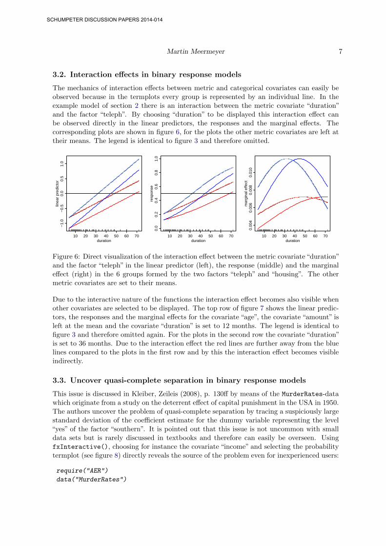
The mechanics of interaction effects between metric and categorical covariates can easily beobserved because in the termplots every group is represented by an individual line. In theexample model of section 2 there is an interaction between the metric covariate “duration”and the factor “teleph”. By choosing “duration” to be displayed this interaction effect canbe observed directly in the linear predictors, the responses and the marginal effects. Thecorresponding plots are shown in figure 6, for the plots the other metric covariates are left attheir means. The legend is identical to figure 3 and therefore omitted.

10 20 30 40 50 60 70

−1.

0−

0.5

0.0

0.5

1.0

duration

linea

r pr

edic

tor

10 20 30 40 50 60 70

0.0

0.2

0.4

0.6

0.8

1.0

duration

resp

onse

10 20 30 40 50 60 70

0.00

40.

006

0.00

80.

010

durationm

argi

nal e

ffect

Figure 6: Direct visualization of the interaction effect between the metric covariate “duration”and the factor “teleph” in the linear predictor (left), the response (middle) and the marginaleffect (right) in the 6 groups formed by the two factors “teleph” and “housing”. The othermetric covariates are set to their means.

Due to the interactive nature of the functions the interaction effect becomes also visible whenother covariates are selected to be displayed. The top row of figure 7 shows the linear predic-tors, the responses and the marginal effects for the covariate “age”, the covariate “amount” isleft at the mean and the covariate “duration” is set to 12 months. The legend is identical tofigure 3 and therefore omitted again. For the plots in the second row the covariate “duration”is set to 36 months. Due to the interaction effect the red lines are further away from the bluelines compared to the plots in the first row and by this the interaction effect becomes visibleindirectly.

3.3. Uncover quasi-complete separation in binary response models

This issue is discussed in Kleiber, Zeileis (2008), p. 130ff by means of the MurderRates-datawhich originate from a study on the deterrent effect of capital punishment in the USA in 1950.The authors uncover the problem of quasi-complete separation by tracing a suspiciously largestandard deviation of the coefficient estimate for the dummy variable representing the level“yes” of the factor “southern”. It is pointed out that this issue is not uncommon with smalldata sets but is rarely discussed in textbooks and therefore can easily be overseen. UsingfxInteractive(), choosing for instance the covariate “income” and selecting the probabilitytermplot (see figure 8) directly reveals the source of the problem even for inexperienced users:

require("AER")

data("MurderRates")



20 30 40 50 60 70

−1.

4−

1.2

−1.

0−

0.8

−0.

6−

0.4

age

linea

r pr

edic

tor

20 30 40 50 60 700.

00.

20.

40.

60.

81.

0age

resp

onse

20 30 40 50 60 70

−0.

0035

−0.

0025

−0.

0015

age

mar

gina

l effe

ct20 30 40 50 60 70

−1.

0−

0.6

−0.

20.

00.

2

age

linea

r pr

edic

tor

20 30 40 50 60 70

0.0

0.2

0.4

0.6

0.8

1.0

age

resp

onse

20 30 40 50 60 70−

0.00

40−

0.00

35−

0.00

30−

0.00

25age

mar

gina

l effe

ct

Figure 7: Indirect visualization of the interaction effect between the metric covariate “du-ration” and the factor “teleph” in the linear predictor (left), the response (middle) and themarginal effect (right) of the metric covariate “age” in the 6 groups formed by the two factors“teleph” and “housing”. For the figures in the first row the covariate “duration” is set to 12months and for the second row to 36 months, the covariate “amount” is set to the mean.

model <- glm(I(executions > 0) ~ time + income + noncauc + lfp + southern,

data = MurderRates, family = binomial)

fxInteractive(model)

southern.nosouthern.yes

1.0 1.5 2.0

0.0

0.2

0.4

0.6

0.8

1.0

income

resp

onse

Figure 8: The probability termplot of a metric covariate, here “income”, uncovers the quasi-complete separation in the MurderRates-data: Observations from the southern states arealways predicted as 1.


Martin Meermeyer 9

4. Details on the text output

The example model from section 2 is used for illustration in this section with the metriccovariates set to their means. The following tables are calculated and printed to the consoleby clicking the Snapshot-button:

• A summary of the model obtained by summary() (not shown).

• Tables of the chosen values of the metric covariates and their ECDF-values (see table 1).

Selected values of metric covariates

amount age duration

value 3271.248 35.542 20.903

ECDF(value) 0.658 0.587 0.554

Table 1: Table of the chosen values of the metric covariates and their ECDF-values.

• In case of limited dependent variable models the table of the link and response functionevaluated for the chosen values of the metric covariates in each group (see table 2).For other regression models the table of the effects for the chosen values of the metriccovariates in each group.

Effects in different groups for selected values of metric covariates

link response

teleph.yes|housing.social -0.4988935 0.3089272

teleph.yes|housing.rent -0.8599626 0.1949048

teleph.yes|housing.freehold -0.4843101 0.3140829

teleph.no|housing.social -0.3219410 0.3737487

teleph.no|housing.rent -0.6830100 0.2473003

teleph.no|housing.freehold -0.3073576 0.3792856

Table 2: Table of the link and response function for the chosen values of the metric covariatesin each group.

• Table of marginal effects for each metric covariate for the chosen values of the metriccovariates in each group (see table 3). In the case of limited dependent variable modelsthe marginal effects refer to the response function. The marginal effects are calculatednumerically with splinefun().

Marginal effects in different groups for selected values of metric covariates

amount age duration

value 3.271248e+03 35.542000000 20.903000000

ECDF(value) 6.580000e-01 0.587000000 0.554000000

teleph.yes|housing.social -2.092170e-05 -0.003687023 0.006380070

teleph.yes|housing.rent -1.637027e-05 -0.002884925 0.004992110

teleph.yes|housing.freehold -2.107224e-05 -0.003713551 0.006425975

teleph.no|housing.social -2.249766e-05 -0.003964754 0.010967026

teleph.no|housing.rent -1.876481e-05 -0.003306914 0.009147355

teleph.no|housing.freehold -2.260113e-05 -0.003982988 0.011017466

Table 3: Table of marginal effects for each metric covariate for the chosen values of the metriccovariates in each group.



When the argument latex2console is set to TRUE in the call of fxInteractive() the tablesare printed to the console as LATEX-code using functions from the package xtable. For thegiven example the tables in appendix A show the results. A LATEX-version of the modelsummaries is not printed to the console. For a number of different fitted-model objects thepackage texreg (Leifeld 2013) provides the functionality to do this.

5. Details on different aspects of usage

The arguments explained in this section control different aspects of usage. The explanationsin this and the following sections are mostly independent of the class of the fitted-model ob-ject provided to fxInteractive(). Some methods however, for instance the “lme”-methodfor linear mixed-effects models, have additional arguments which are described in the corre-sponding documentation. The probit model from section 2 is used as example throughoutthis section.

Exact control over metric covariates With the sliders the values of the metric covariatescannot be selected with arbitrary precision. To allow exact control over the values these canbe set as initial values for the sliders with the argument initial.values through a namedlist. The names in the list must exactly match the variable names:

fxInteractive(model.2.fac,

initial.values = list(amount=5000, duration=24, age=30))

If a metric covariate is not explicitly listed the corresponding slider is initialized with themean (the default).

Preselect metric covariate, plot type and groups To avoid the appearance of theselection menu the name of the metric covariate to be displayed can be preselected:

fxInteractive(model.2.fac, preselect.var = "duration")

If no metric covariate with the provided name exists the selection menu will pop up instead.

The type of plot to be displayed first can also be specified by the argument preselect.type.The possible values depend on the class of the fitted-model object, please refer to the docu-mentation of the corresponding method. For the “glm”-method for example this must be oneof the values "link" (the default), "response" or "marginal":

fxInteractive(model.2.fac, preselect.type = "response")

By default all groups are active in the initial plot. With the argument preselect.groups

the groups displayed in the initial plot can be specified with a numeric index vector. The firstthree groups are preselected by

fxInteractive(model.2.fac, preselect.groups = c(1:3))

Preselecting groups is useful if the model contains many factors. In this case the panelusually grows beyond the screen and some groups are not accessible via the GUI-panel any


Martin Meermeyer 11

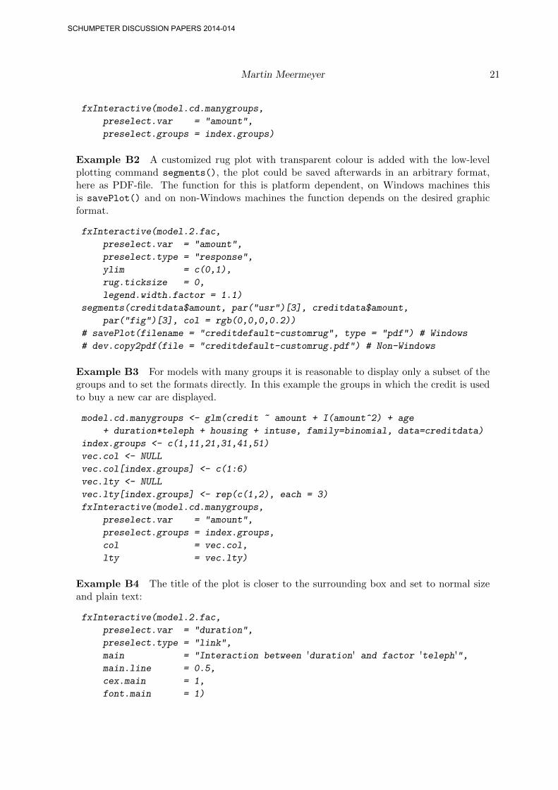
more. The groups are constructed with the function factorCombinations() which can beused to identify groups of interest. This is illustrated in example B1 in appendix B.

The functionality to prespecify the variable, the plot type and certain groups in advance isbeneficial when used in conjunction with the argument initial.values and the automaticsave functionality. All taken together, this allows the reproduction of plots without userinteraction, see the last example in this section.

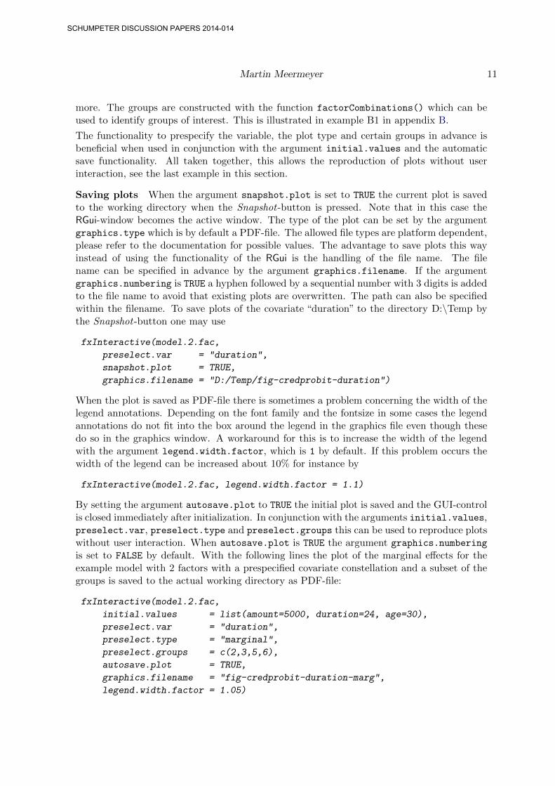
Saving plots When the argument snapshot.plot is set to TRUE the current plot is savedto the working directory when the Snapshot-button is pressed. Note that in this case theRGui-window becomes the active window. The type of the plot can be set by the argumentgraphics.type which is by default a PDF-file. The allowed file types are platform dependent,please refer to the documentation for possible values. The advantage to save plots this wayinstead of using the functionality of the RGui is the handling of the file name. The filename can be specified in advance by the argument graphics.filename. If the argumentgraphics.numbering is TRUE a hyphen followed by a sequential number with 3 digits is addedto the file name to avoid that existing plots are overwritten. The path can also be specifiedwithin the filename. To save plots of the covariate “duration” to the directory D:\Temp bythe Snapshot-button one may use


preselect.var = "duration",

snapshot.plot = TRUE,

graphics.filename = "D:/Temp/fig-credprobit-duration")

When the plot is saved as PDF-file there is sometimes a problem concerning the width of thelegend annotations. Depending on the font family and the fontsize in some cases the legendannotations do not fit into the box around the legend in the graphics file even though thesedo so in the graphics window. A workaround for this is to increase the width of the legendwith the argument legend.width.factor, which is 1 by default. If this problem occurs thewidth of the legend can be increased about 10% for instance by

fxInteractive(model.2.fac, legend.width.factor = 1.1)

By setting the argument autosave.plot to TRUE the initial plot is saved and the GUI-controlis closed immediately after initialization. In conjunction with the arguments initial.values,preselect.var, preselect.type and preselect.groups this can be used to reproduce plotswithout user interaction. When autosave.plot is TRUE the argument graphics.numbering

is set to FALSE by default. With the following lines the plot of the marginal effects for theexample model with 2 factors with a prespecified covariate constellation and a subset of thegroups is saved to the actual working directory as PDF-file:


initial.values = list(amount=5000, duration=24, age=30),


preselect.type = "marginal",

preselect.groups = c(2,3,5,6),

autosave.plot = TRUE,

graphics.filename = "fig-credprobit-duration-marg",

legend.width.factor = 1.05)



On Windows systems the legend width needs to be increased for the PDF-files to look asexpected. The figures of section 3 are created in this reproducible way, the code can be foundin the demo of the package.

6. Details on customization

The appearance of the text output, the plots and the GUI-controls can be customized in manyways. The arguments for the methods for the different classes of fitted-model object are almostidentical. If the arguments vary along the methods this will be mentioned. Two probit modelsare used for demonstration throughout this section. Firstly the model introduced in section 2:

data("creditdata")



Additionally the following probit model with 3 metric covariates and 3 factors with 2, 3 and4 levels respectively is also used occasionally:

data("creditdata")


+ housing + job, family = binomial(link="probit"), data = creditdata)

6.1. Customize text output

Separation characters in group names Within the group names which are used in thelegend and the text output the character separating the factor name and the correspondingfactor levels can be set with the argument level.sep (default to“.”). The character separatingfactor-factor level combinations can be set with the argument factor.sep (default to “|”).Another reasonable pair of separation characters is for instance


factor.sep = "-",

level.sep = ">")

Decimal mark and big mark in LATEX-output The LATEX-output is generated by thefunctions xtable() and the corresponding method print.xtable() from the package xtable.The appearance of the output is controlled by five arguments which are directly passed tothese functions. With the arguments xtable.big.mark and xtable.decimal.mark the bigmark and decimal mark characters can be set. By default xtable() uses 2 digits, whichcan be changed with the argument xtable.digits. The overall format of the numberscan be controlled with the argument xtable.display, please refer to the documentation ofxtable() for possible values. If the horizontal lines should be set with commands from theLATEX-package booktabs the argument xtable.booktabs must be set to TRUE. Changing theLATEX-output to the continental European number format with 5 digits and using horizontallines from the booktabs-package can be achieved by


Martin Meermeyer 13


latex2console = TRUE,

xtable.big.mark = ".",

xtable.decimal.mark = ",",

xtable.digits = 5,

xtable.booktabs = TRUE)

For the LATEX-code printed to the console the following preamble (here prepared for Germanlanguage) for a utf8-encoded TEX-file works well:

\documentclass[a4paper]{scrartcl}

\usepackage[T1]{fontenc}

\usepackage[utf8]{inputenx}

\usepackage[ngerman]{babel}

\usepackage[babel,german=quotes]{csquotes}

\usepackage{icomma}

\usepackage{booktabs}

\begin{document}

% copy and paste from R Console}

\end{document}

6.2. Customize graphic device

Many graphical elements can be controlled directly by arguments in the function call. Themajor appearance of the plots can be controlled by the manipulation of par()-arguments. Ifnecessary graphical elements can be added to the plots by low-level plotting commands in theR Console. Note that elements added this way are not captured by the autosave functionalitydescribed at the end of section 5. The example B2 in appendix B shows how to save plotswithout user interaction in this case.

Plot dimensions and pointsize The dimensions of the graphic device (in centimeters)and the pointsize of plotted text can be set. A more compact plot is for instance obtained by:


dev.height = 11,

dev.width = 11,

dev.width.legend = 5,

dev.pointsize = 8)

When a legend is added the overall width of the device is dev.width plus dev.width.legend.By default a legend is added when at least one factor is used as covariate. For more detailson the legend refer to the paragraph “Legend” in this section.

Vertical limits of the plot The vertical limits of the plots are determined automaticallyby default. If this is not desired the limits can be set manually with the usual ylim-argument.For the response function of the example probit model it is reasonable to set the limits to 0and 1:




preselect.var = "amount",

preselect.type = "response",

ylim = c(0,1))

Note that the vertical limits apply to every kind of plot. Therefore it is usually advisable tofix the limits only if the plots are saved automatically, see section 5 for details on this.

Colours, line types and line widths The colours, line types and line widths for the linesrepresenting different groups in the plots and the legend can be set directly. For the modelwith 2 factors the following scheme is suitable:


col = c(1,"blue",2),

lwd = rep(c(1,2),each=3))

Note that the arguments are recycled if necessary, in this case for the colour. The levels of thefactor “teleph” are represented by the thickness of lines and the levels of the factor “housing”by the colour. For the model with 3 factors one may use


col = rep(c(1,"blue",2), each=4),

lty = c(1,2,3,4),

lwd = rep(c(1,2), each=12),

dev.width.legend = 8)

The levels of the additional factor “job” are represented by the line type here. The visualdiscrimination of 4 or more factors will be conceptually hard to achieve. In this case it maybe advisable to display only a subset of groups by deselecting the complement groups in thecheckbox or by using the argument preselect.groups. If just a subset of groups is displayedit is convenient to set the line formats directly, see the example B3 in appendix B how to dothis.

Title and axis labels By default no title is added to the plot, the label for the x -axis isthe name of the selected covariate and the label for the y-axis is the name of the selected plottype. This can be overridden if necessary, for instance with more detailed annotations:




main = "Interaction between 'duration' and factor 'teleph'",xlab = "duration (months)",

ylab = "probability of credit default")

The argument main is passed to the function title() which allows to control the vertical po-sition of the headline, the corresponding argument is main.line. In appendix B the exampleB4 shows to customize the title.


Martin Meermeyer 15

Legend A legend is added by default when at least one categorical covariate is used. Thelegend is plotted within an own region with the left and right margin of the legend regionset to 0. The legend frequently needs to be modified since the space required by the legenddepends on the number of factors used as covariates, the lengths of the group names, thephysical screen resolution and the size of the RGui-window (if run in MDI-mode, not relevantfor users of RStudio). On the one hand the space for the legend itself can be modified andon the other hand the scaling of the legend. The first solution for the example model with 3factors is

fxInteractive(model.3.fac, dev.width.legend = 8)

For the same model reducing the scale to 70% of the original size also works:

fxInteractive(model.3.fac, legend.cex = 0.7)

The position of the legend can be modified as well, refer to the documentation of legend()for details:

fxInteractive(model.2.fac, legend.pos = "top")

With the argument legend.width.factor the width of the box around the legend can bemanipulated, see the explanations in the paragraph “Saving plots” in section 5.

When factors are present the legend and the corresponding plot region for it can be completelysuppressed by

fxInteractive(model.2.fac, legend.add = FALSE)

Setting the additional argument legend.space to TRUE will create the corresponding plotregion without the legend:


legend.add = FALSE,

legend.space = TRUE)

This can be useful if different plots are arranged in a document but for only one of theplots a legend should appear. The empty spaces ensure exact alignments and matching plotdimensions in this case. Figure 3 in section 3 is an example for this, the code to reproduce thefigure can be found in the demo of the package. To achieve full flexibility for the arrangementof plots in a document the legend can be plotted alone:

fxInteractive(model.2.fac, legend.only = TRUE)

Since the legend is the only element within the plotting region in this case it is usuallyreasonable to set the margins to 0 with the additional argument mar=c(0,0,0,0). Note thatthe width of the graphic device is solely controlled by dev.width.legend and in conjunctionwith dev.height the overall size of the legend can be set precisely.



Rug plot By default a rug representation of the selected metric covariate is added to thesouthern axis of the plot. The length of the ticks can be controlled with the argumentrug.ticksize which is 0.02 by default. For many observations the rug considerably slowsdown the rebuild of the plot. Setting rug.ticksize to 0 or NA removes the rug representation:

fxInteractive(model.2.fac, rug.ticksize = NA)

The colour of the rug tickmarks can be changed with the argument rug.col:

fxInteractive(model.2.fac, rug.col = "gray50")

If more detailed control over the rug is needed, the rug needs to be suppressed and addedwith rug() from the R Console. The example B2 in section B shows how to add a customizedrug plot with transparent colours.

Vertical and horizontal lines To facilitate visual perception a few straight lines are addedto the plots by default. A vertical black line shows the actual value of the selected metriccovariate. To suppress the vertical line, e.g. for printing the plot, use

fxInteractive(model.2.fac, vline.actual = FALSE)

By default horizontal black lines are added to the different plots, the vertical positions of thelines can be controlled with the argument pos.hlines. The argument has to be a numericvector with the vertical positions of the lines. The length of the vector and the defaultvalues depend on the class of the fitted-model object, please refer to the documentation of thecorresponding method for details. For the “glm”-method the default is for instance the vectorc(0,0.5,0) giving horizontal lines in the plot of the linear predictors at height 0, in the plotof the responses at height 0.5 and in the plot of the marginal effects at height 0. Each linecan be suppressed by setting the corresponding value to NA. For instance suppressing the linefor the link function and setting the line in the plot of the response to 0.56 can be achievedby

fxInteractive(model.2.fac, pos.hlines = c(NA,0.56,0))

The appearance of the lines (solid black lines) cannot be changed by arguments. To modifythis the lines these must be suppressed and added with abline()-commands afterwards.

Number of points used for plotting The effects are plotted for a sequence of equallyspaced points over the span of the chosen metric covariate. With the argument n.effects

the number of points can be controlled (default to 100). If the lines of the effects are notsmooth this value can be increased.

6.3. Predefining the graphic device

For more control over the appearance of the plots the graphic device can be specified inadvance. Two plot regions which can be accessed with high-level plotting commands arerequired. The legend is plotted in the first region and the plot itself in the second region toallow the user to add elements to an existing plot with low-level plotting commands. Theleft and right margin of the legend region are set to 0. In the following example the legend


Martin Meermeyer 17

appears on the left side, the colours are specified via palette() and the margins as well asthe scale of the text are changed. Note that for pointsize 10 the width of the legend must beincreased to achieve that the legend annotations fit into the box of the legend in the PDF-file.

windows(10,7, pointsize = 10)

layoutmatrix <- matrix(c(1,2,2), 1, 3)

layout(layoutmatrix)

palette(c("darkred","red","salmon","darkblue","blue","lightblue"))

par(cex = 1, mar = c(5,5,2,2)+0.1)




dev.defined = TRUE,

ylim = c(0,1),

legend.width.factor = 1.1,

snapshot.plot = TRUE)

6.4. Customize GUI-controls

Size of the GUI-controls The size of the entire panel is calculated automatically andprimarily depends on the number of covariates and groups but also on the screen resolution.Because of this the results from the automatic calculation are sometimes not to 100% satis-factory, therefore the layout of the panel can be modified by a number of parameters. Thiscan be useful for screens with a low resolution or if the model has a lot of groups. For thelatter case the parameters are changed in the following example to save space:


box.type.height = 90,

box.group.character.width = 6,

box.group.line.height = 25,

dist.obj.height = 2)

Note that for a large number of groups not every group can be seen in the GUI-panel becausethe panel grows beyond the screen margin. In former versions of rpanel (< 1.1-3) the entriesof the checkbox are squeezed together. Currently there is no way to circumvent this problem.At the moment the only solution is to choose the groups in advance using the argumentpreselect.groups, see the paragraph “Preselect metric covariate, plot type and groups” insection 5.

Annotations of the GUI-controls The annotations of the GUI-controls can be changedeasily, for instance to German:


panel.title = "Probit Modell",

label.button = "Schnappschuss",

label.slider.act = "Dargestellte Variable: ",

label.box.type = "Typ",



label.types = c("Linearer Praediktor", "Wahrscheinlichkeit",

"Marginaler Effekt"),

label.box.groups = "Gruppen")

Note that the label.types for the annotations of the radiobox are used as default annotationsfor the y-axis of the corresponding plots. The length of the character vector and the defaultentries for this argument depend on the class of the fitted-model object, please refer to thedocumentation of the corresponding method for details. For the “glm”-method for instance acharacter vector of length 3 to annotate the radiobox choices for the plot of the link functions,the response functions and the marginal effects is required.

7. Solving problems with raw data extraction

The internal calculations are based on the prediction method of the fitted-model object andthe raw data. Internally it is tried to extract the raw data with get_all_vars(model$terms,

model$data). If the fitted-model object lacks a data slot, it is tried to retrieve the rawdata with get_all_vars(model$terms, model$model). For example fitted-model objects ofclass “lm” lack a data slot and for some formulas the latter extraction method does not workproperly, for instance if a covariate is incorporated as spline function via bs(). Adding a data

slot to the fitted-model object afterwards solves this particular problem. This is demonstratedby means of a linear regression model for the rents of apartments in Munich, Germany. Thedataset munichrent03 is contained in the package and was originally obtained from the DataArchive of the Department of Statistics, University of Munich and of the SFB 386 (2014b).The variables are described in the documentation of the dataset munichrent03:

data("munichrent03")

require("splines")

model.rent <- lm(rent ~ bs(yearc) + area*location + upkitchen,

data=munichrent03)

model.rent$data <- munichrent03

fxInteractive(model.rent)

Adding a data slot afterwards may also be helpful if the raw data cannot be extracted forother reasons.

References

Bowman A, Crawford E, Alexander G, Bowman R (2007). “rpanel: Simple Interactive Con-trols for R Functions Using the tcltk package.” Journal of Statistical Software, 17(9), 1–18.

Bowman A, Gibson L, Scott M, Crawford E (2010). “Interactive Teaching Tools for SpatialSampling.” Journal of Statistical Software, 36(13), 1–17.

Dahl DB (2014). xtable: Export tables to LaTeX or HTML. R package version 1.7-4, URLhttp://CRAN.R-project.org/package=xtable.


http://CRAN.R-project.org/package=xtable

Martin Meermeyer 19

Data Archive of the Department of Statistics, University of Munich and of the SFB 386(2014a). Dataset ”Kreditscoring zur Klassifikation von Kreditnehmern”. URL http://www.

stat.uni-muenchen.de/service/datenarchiv/kredit/kredit.html.

Data Archive of the Department of Statistics, University of Munich and of the SFB 386(2014b). Dataset ”Munchner Mietspiegel 2003”. URL http://www.stat.uni-muenchen.

de/service/datenarchiv/miete/miete03.html.

Fernihough A (2014). mfx: Marginal Effects, Odds Ratios and Incidence Rate Ratios forGLMs. R package version 1.1, URL http://CRAN.R-project.org/package=mfx.

Fox J (2003). “Effect Displays in R for Generalised Linear Models.” Journal of StatisticalSoftware, 8(15), 1–27.

Hastie T (2013). gam: Generalized Additive Models. R package version 1.09.1, URL http:

//CRAN.R-project.org/package=gam.

Hoetker G (2007). “The Use of Logit and Probit Models in Strategic Management Research:Critical Issues.” Strategic Management Journal, 28(4), 331–343.

Leifeld P (2013). “texreg: Conversion of Statistical Model Output in R to LATEX and HTMLTables.” Journal of Statistical Software, 55(8), 1–24. URL http://www.jstatsoft.org/

v55/i08/.

Meermeyer M (2014). LinRegInteractive: Interactive Interpretation of Linear Regres-sion Models. R package version 0.2-3, URL http://CRAN.R-project.org/package=

LinRegInteractive.

R Core Team (2014). R: A Language and Environment for Statistical Computing. R Founda-tion for Statistical Computing, Vienna, Austria. URL http://www.R-project.org/.

Wood S (2014). mgcv: Mixed GAM Computation Vehicle with GCV/AIC/REML SmoothnessEstimation. R package version 1.8-0, URL http://CRAN.R-project.org/package=mgcv.

Xie Y (2013). “Animation: An R Package for Creating Animations and Demonstrating Sta-tistical Methods.” Journal of Statistical Software, 53(1), 1–27.


http://www.stat.uni-muenchen.de/service/datenarchiv/kredit/kredit.html

http://www.stat.uni-muenchen.de/service/datenarchiv/kredit/kredit.html

http://www.stat.uni-muenchen.de/service/datenarchiv/miete/miete03.html

http://www.stat.uni-muenchen.de/service/datenarchiv/miete/miete03.html

http://CRAN.R-project.org/package=mfx

http://CRAN.R-project.org/package=gam

http://CRAN.R-project.org/package=gam

http://www.jstatsoft.org/v55/i08/

http://www.jstatsoft.org/v55/i08/

http://CRAN.R-project.org/package=LinRegInteractive

http://CRAN.R-project.org/package=LinRegInteractive

http://www.R-project.org/

http://CRAN.R-project.org/package=mgcv


A. Example of LATEX text output

The three tables together with the captions in this section are the text output (see section 4)for the model given in section 2 with the argument latex2console set to TRUE and theargument xtable.digits set to 5.

amount age duration

value 3.271,24800 35,54200 20,90300ECDF(value) 0,65800 0,58700 0,55400

Table 4: Selected values of metric covariates

link response

teleph.yes|housing.social -0,49889 0,30893teleph.yes|housing.rent -0,85996 0,19490teleph.yes|housing.freehold -0,48431 0,31408teleph.no|housing.social -0,32194 0,37375teleph.no|housing.rent -0,68301 0,24730teleph.no|housing.freehold -0,30736 0,37929

Table 5: Effects in different groups for selected values of metric covariates

amount age duration

value 3.271,24800 35,54200 20,90300ECDF(value) 0,65800 0,58700 0,55400

teleph.yes|housing.social -0,00002 -0,00369 0,00638teleph.yes|housing.rent -0,00002 -0,00288 0,00499teleph.yes|housing.freehold -0,00002 -0,00371 0,00643teleph.no|housing.social -0,00002 -0,00396 0,01097teleph.no|housing.rent -0,00002 -0,00331 0,00915teleph.no|housing.freehold -0,00002 -0,00398 0,01102

Table 6: Marginal effects in different groups for selected values of metric covariates

B. Additional examples

Example B1 For models with many groups the GUI-panel grows beyond the screen. Theonly way to select or deselect the nonvisible groups is to preselect these. In this example onlythe groups which occur more than 10 times in the data are choosen to be displayed.

model.cd.manygroups <- glm(credit ~ amount + I(amount^2) + age

+ duration*teleph + housing + intuse, family=binomial, data=creditdata)

factor.combs <- factorCombinations(creditdata[,c("teleph",

"housing","intuse")])

logic.index.groups <- factor.combs$counts > 10

index.groups <- seq(along=factor.combs$counts)[logic.index.groups]


Martin Meermeyer 21

fxInteractive(model.cd.manygroups,


preselect.groups = index.groups)

Example B2 A customized rug plot with transparent colour is added with the low-levelplotting command segments(), the plot could be saved afterwards in an arbitrary format,here as PDF-file. The function for this is platform dependent, on Windows machines thisis savePlot() and on non-Windows machines the function depends on the desired graphicformat.




ylim = c(0,1),

rug.ticksize = 0,

legend.width.factor = 1.1)

segments(creditdata$amount, par("usr")[3], creditdata$amount,

par("fig")[3], col = rgb(0,0,0,0.2))

# savePlot(filename = "creditdefault-customrug", type = "pdf") # Windows

# dev.copy2pdf(file = "creditdefault-customrug.pdf") # Non-Windows

Example B3 For models with many groups it is reasonable to display only a subset of thegroups and to set the formats directly. In this example the groups in which the credit is usedto buy a new car are displayed.

model.cd.manygroups <- glm(credit ~ amount + I(amount^2) + age

+ duration*teleph + housing + intuse, family=binomial, data=creditdata)

index.groups <- c(1,11,21,31,41,51)

vec.col <- NULL

vec.col[index.groups] <- c(1:6)

vec.lty <- NULL

vec.lty[index.groups] <- rep(c(1,2), each = 3)

fxInteractive(model.cd.manygroups,


preselect.groups = index.groups,

col = vec.col,

lty = vec.lty)

Example B4 The title of the plot is closer to the surrounding box and set to normal sizeand plain text:



preselect.type = "link",

main = "Interaction between 'duration' and factor 'teleph'",main.line = 0.5,

cex.main = 1,

font.main = 1)



Affiliation:

Martin MeermeyerBergische Universitat WuppertalSchumpeter School of Business and EconomicsGaussstr. 2042119 Wuppertal, GermanyE-mail: [email protected]: http://www.statistik.uni-wuppertal.de


mailto:[email protected]

http://www.statistik.uni-wuppertal.de

SCHUMPETER DISCUSSION PAPERS LinRegInteractive: An...

Documents

Transcript of SCHUMPETER DISCUSSION PAPERS LinRegInteractive: An...