SCHOOL OF SIENCE AND HUMANITIES DEPARTMENT OF …
70
SCHOOL OF SIENCE AND HUMANITIES DEPARTMENT OF MATHEMATICS Course Objectives: To motivate the students to apply the concepts and methods of differential equations to solve complex problems. Course Outcomes: At the end of the course, the student will be able to: CO1 Define Order, degree of ODE and PDE. Identify the methods to solve homogeneous and non-homogeneous ODE and PDE. CO2 Classify ODE and PDE. Illustrate various methods to solve second order Differential equation and Partial differential equations. CO3 Solve some special types of partial differential equations by Charpit’s and Jacobi’s method. CO4 Analyze the solution of first order differential equations by various methods. CO5 Evaluate higher order differential equations by method of variation of parameters. CO6 Formation of ODE & PDE for the given function. Syllabus Unit I Differential Equations of First Order Elementary Methods in Ordinary Differential Equations. Formation of differential equation. Solutions: General, particular, and singular. First order exact equations and integrating factors. Degree and order of a differential equation. Equations of first order and first degree. Equations in which the variable are separable. Homogeneous equations. First order higher degree equations solvable for x, y, p. Clairaut's form and singular solutions. Linear differential equations with constant coefficients. Homogeneous linear ordinary differential equations. Unit II Differential Equations of Second Order Linear differential equations of second order. Second order equation with constant coefficient with particular integrals for e ax , x m , e ax sinmx, e ax cosmx. Method of variation of parameters. Ordinary simultaneous differential equations.
Transcript of SCHOOL OF SIENCE AND HUMANITIES DEPARTMENT OF …

SCHOOL OF SIENCE AND HUMANITIES
DEPARTMENT OF MATHEMATICS
Course Objectives:
To motivate the students to apply the concepts and methods of differential equations to solve
complex problems.
Course Outcomes: At the end of the course, the student will be able to:
CO1 Define Order, degree of ODE and PDE. Identify the methods to solve homogeneous and
non-homogeneous ODE and PDE.
CO2 Classify ODE and PDE. Illustrate various methods to solve second order Differential
equation and Partial differential equations.
CO3 Solve some special types of partial differential equations by Charpit’s and Jacobi’s method.
CO4 Analyze the solution of first order differential equations by various methods.
CO5 Evaluate higher order differential equations by method of variation of parameters.
CO6 Formation of ODE & PDE for the given function.
Syllabus
Unit I Differential Equations of First Order
Elementary Methods in Ordinary Differential Equations. Formation of differential equation.
Solutions: General, particular, and singular. First order exact equations and integrating factors.
Degree and order of a differential equation. Equations of first order and first degree. Equations
in which the variable are separable. Homogeneous equations. First order higher degree equations
solvable for x, y, p. Clairaut's form and singular solutions. Linear differential equations with
constant coefficients. Homogeneous linear ordinary differential equations.
Unit II Differential Equations of Second Order
Linear differential equations of second order. Second order equation with constant coefficient
with particular integrals for eax, xm, eaxsinmx, eaxcosmx. Method of variation of parameters.
Ordinary simultaneous differential equations.

Unit III Partial Differential Equation
Partial differential equations. Formation of partial differential equations. Types of solutions.
PDEs of the first order. Lagrange's solution.
Unit IV Partial Differential Equation (Contd…)
Some special types of equations which can be solved easily by methods other than the general
methods. Charpit's and Jacobi's general method of solution.
Unit V Second and Higher Order Partial Differential Equation
Partial differential equations of second and higher order. Classification of linear partial
differential equations of second order. Homogeneous and non-homogeneous equations with
constant coefficients. Partial differential equations reducible to equations with constant
coefficients.

UNIT – I – Ordinary and Partial Differential Equations – SMTA1305
Unit I
Differential Equations of First Order
Topics covered in this unit are: Definition of an ordinary differential equation, Degree and order
of a differential equation, Formation of differential equations, Solutions: General, particular, and
singular, First order exact equations and integrating factors, Equations in which the variable are
separable, Homogeneous equations, Equations of first order and first degree, Linear equations
and equations reducible to linear form, First order higher degree equations solvable for x, y, p,
Clairaut's form and singular solutions, Orthogonal trajectories.
1 Introduction to Ordinary Differential Equations (ODE)
1.1 Definition
A differential equation is an equation which involves differentials or differential coefficients.
Differential equation is an equation involving one or more functions with its derivatives. The
derivatives of the function define the rate of change of a function. Differential equations are
used to model physical phenomena that involves rate of change.
Examples: (i) 𝑑2𝑦
𝑑𝑥2 + 2𝑑𝑦
𝑑𝑥+ 𝑦 = 𝑠𝑖𝑛𝑥 (ii)
𝑑𝑦
𝑑𝑥= 𝑥2.
1.2 Order and Degree of a ODE
Order is the highest derivative present in the differential equation and degree is the exponent
of the highest derivative.
Example: In (𝑑2𝑦
𝑑𝑥2)3
+ 2 (𝑑𝑦
𝑑𝑥)
2
+ 𝑦 = 2, Order = 2 and Degree = 3.
2 Formation of Ordinary Differential Equations
The following are the steps involved in forming a ODE:
Given the general solution of a ODE in the form 𝑓(𝑥, 𝑦, 𝑐1, 𝑐2, … , 𝑐𝑛) = 0_____(1)
Step 1: Find the number of arbitrary constants ‘n’ present in equation (1).
Step 2: Differentiate (1) w.r.t. independent variable x, present in (1).
Step 3: Keep differentiating ‘n’ times, so that (n+1) equations are obtained.
Step 4: Using the (n+1) equations are obtained, eliminate the constants 𝑐1, 𝑐2, … , 𝑐𝑛.
Example 1
Construct an ordinary differential equation whose general solution is 𝑦 = 𝐴𝑒2𝑥 + 𝐵𝑒−2𝑥.
Solution.
Given 𝑦 = 𝐴𝑒2𝑥 + 𝐵𝑒−2𝑥_______________(1)
Since there are two arbitrary constants A and B, we differentiate (1) twice.
𝑦1 = 2𝐴𝑒2𝑥 − 2𝐵𝑒−2𝑥_______________(2)
𝑦2 = 4𝐴𝑒2𝑥 + 4𝐵𝑒−2𝑥_______________(3)
This implies that 𝑦2 = 4(𝐴𝑒2𝑥 + 𝐵𝑒−2𝑥).

⟹ 𝑦2 = 4𝑦
Therefore, 𝑑2𝑦
𝑑𝑥2 − 4𝑦 = 0 is the required ODE.
Example 2
Construct a differential equation whose general solution is 𝑦 = 𝐴𝑒𝑥 + 𝐵𝑒2𝑥 + 𝐶𝑒−3𝑥.
Solution.
Given 𝑦 = 𝐴𝑒𝑥 + 𝐵𝑒2𝑥 + 𝐶𝑒−3𝑥_______________(1)
Since there are three arbitrary constants A, B and C, we differentiate (1) thrice.
𝑦1 = 𝐴𝑒𝑥 + 2𝐵𝑒2𝑥 − 3𝐶𝑒−3𝑥_______________(2)
𝑦2 = 𝐴𝑒𝑥 + 4𝐵𝑒2𝑥 + 9𝐶𝑒−3𝑥_______________(3)
𝑦3 = 𝐴𝑒𝑥 + 8𝐵𝑒2𝑥 − 27𝐶𝑒−3𝑥_______________(4)
First we eliminate A from (1), (2), (3) and (4).
(2) − (1) ⟹ 𝑦1 − 𝑦 = 𝐵𝑒2𝑥 − 4𝐶𝑒−3𝑥.
(3) − (2) ⟹ 𝑦2 − 𝑦1 = 2𝐵𝑒2𝑥 + 12𝐶𝑒−3𝑥.
(2) − (1) ⟹ 𝑦3 − 𝑦2 = 4𝐵𝑒2𝑥 − 36𝐶𝑒−3𝑥.
We then eliminate Band C, by using the determinant,
|
𝑦1 − 𝑦 𝐵 −4𝐶𝑦2 − 𝑦1 2𝐵 12𝐶𝑦3 − 𝑦2 4𝐵 −36𝐶
| = 0
⟹ |
𝑦1 − 𝑦 1 1𝐶𝑦2 − 𝑦1 2 3𝐶𝑦3 − 𝑦2 4 9𝐶
| = 0
Expanding the determinant we get,
7𝑦1 − 6𝑦 − 𝑦3 = 0
or,
𝑦3 − 7𝑦1 + 6𝑦 = 0.
⟹𝑑3𝑦
𝑑𝑥3− 7
𝑑𝑦
𝑑𝑥+ 6𝑦 = 0 is the required ODE.
3 Types of Solution of a ODE
Solution: Any relation connecting the variables of an equation and not involving their
derivatives, which satisfies the given differential equation is called a solution.
General Solution: A solution of a differential equation in which the number of arbitrary
constants is equal to the number of independent variables in the equation is called a general
or complete solution or complete primitive of the equation.

Example: 𝑦 = 𝐴𝑥 + 𝐵.
Particular Solution: The solution obtained by giving particular values to the arbitrary
constants of the general solution, is called a particular solution of the equation.
Example: 𝑦 = 3 𝑥 + 5.
Singular Solution: A solution of a differential equation in which contains no arbitrary
constants is called the singular solution.
4 Exact Linear Differential Equations
A differential equation of the type 𝑀𝑑𝑥 + 𝑁𝑑𝑦 = 0 is called an exact differential equation
where 𝑀 and 𝑁 are functions of x and y if and only if 𝑀𝑦 = 𝑁𝑥. The solution of an exact
differential equation is of the form 𝐹(𝑥, 𝑦) = 𝑐, where 𝑐 is an arbitrary constant.
The following are the steps involved in solving an exact equation:
Step 1: Test the exactness of the given equation.
Step 2: Write the general solution as 𝐹(𝑥, 𝑦) = 𝑐 where 𝐹𝑥 = 𝑀 and 𝐹𝑦 = 𝑁.
Step 3: Integrate 𝐹 w.r.t. x and y and write the constants in terms of g(y) and h(x).
Step 4: Compare 𝐹 and find g(y) and h(x).
Step 5: Substitute 𝐹 in Step 2 which is the general solution.
Example 3
Solve 4𝑥𝑠𝑖𝑛𝑦𝑑𝑥 + 2𝑥2𝑐𝑜𝑠𝑦𝑑𝑦 = 0.
Solution.
Let 𝑀 = 4𝑥𝑠𝑖𝑛𝑦 and 𝑁 = 2𝑥2𝑐𝑜𝑠𝑦.
⟹ 𝑀𝑦 = 4𝑥𝑐𝑜𝑠𝑦 and 𝑁𝑥 = 4𝑥𝑐𝑜𝑠𝑦
⟹ 𝑀𝑦 = 𝑁𝑥.
⟹The given equation is exact.
Therefore, the general solution is 𝐹(𝑥, 𝑦) = 𝑐_____(1), where 𝐹𝑥 = 𝑀 and 𝐹𝑦 = 𝑁.
⟹ 𝐹𝑥 = 4𝑥𝑠𝑖𝑛𝑦 and 𝐹𝑦 = 2𝑥2𝑐𝑜𝑠𝑦.
Integrating 𝐹 w.r.t x and y, we get, 𝐹 = 2𝑥2𝑠𝑖𝑛𝑦.
Substituting 𝐹 in equation (1),
2𝑥2𝑠𝑖𝑛𝑦 = 𝑐 is the general solution of the given differential equation.
Example 4
Solve (3𝑥2𝑦 − 6𝑥)𝑑𝑥 + (𝑥3 + 2𝑦)𝑑𝑦 = 0.
Solution.
Let 𝑀 = 3𝑥2𝑦 − 6𝑥 and 𝑁 = 𝑥3 + 2𝑦.
⟹ 𝑀𝑦 = 3𝑥2 and 𝑁𝑥 = 3𝑥2
⟹ 𝑀𝑦 = 𝑁𝑥.
⟹The given equation is exact.

Therefore, the general solution is 𝐹(𝑥, 𝑦) = 𝑐_____(1), where 𝐹𝑥 = 𝑀 and 𝐹𝑦 = 𝑁.
⟹ 𝐹𝑥 = 3𝑥2 − 6𝑥 and 𝐹𝑦 = 𝑥3 + 2𝑦.
Integrating 𝐹 w.r.t x and y, we get, 𝐹 = 𝑥3𝑦 − 3𝑥2 + 𝑦2.
Substituting 𝐹 in equation (1),
𝑥3𝑦 − 3𝑥2 + 𝑦2 = 𝑐 is the general solution of the given differential equation.
5 Separable Equations
A first order differential equation 𝑦′ = 𝑓(𝑥, 𝑦) is called a separable equation if the function
𝑓(𝑥, 𝑦) can be factorised into two functions 𝑔(𝑦) and ℎ(𝑥). The following are the steps involved
in solving separable equations:
Step 1: Check whether the given equation is separable.
Step 2: Separate the variables y and dy to the LHS and those of x and dx to the RHS.
Step 3: Integrate on both sides to get the general solution.
Step 4: To find the particular solution, substitute the initial conditions in the general solution.
Example 5
Solve 𝑑𝑦
𝑑𝑥=
2𝑥
3𝑦2.
Solution.
The given differential equation is separable.
Therefore, 3𝑦2𝑑𝑦 = 2𝑥𝑑𝑥.
Integrating on both sides, we get,
𝑦3 = 𝑥2 + 𝐶.
⟹ 𝑦 = (𝑥2 + 𝐶)1
3 is the general solution.
Example 6
Solve 𝑦′ = 𝑦2𝑠𝑖𝑛𝑥.
Solution.
Given equation can be written as 𝑑𝑦
𝑑𝑥= 𝑦2𝑠𝑖𝑛𝑥.
The given differential equation is separable.
Therefore, 𝑑𝑦
𝑦2= 𝑠𝑖𝑛𝑥𝑑𝑥.
Integrating on both sides, we get, 1
𝑦= 𝑐𝑜𝑠𝑥 + 𝐶.
⟹ 𝑦 =1
𝑐𝑜𝑠𝑥+𝐶 is the general solution.
6 Homogeneous Equations
An expression is said to be homogeneous if the degree of the variables (or the sum of the powers
of different variables) in each term is the same.
Examples: 2𝑥 + 5𝑦, 5𝑥2 − 3𝑥𝑦 + 4𝑦2.

An homogeneous differential equation is of the form 𝑑𝑦
𝑑𝑥=
𝑓(𝑥,𝑦)
𝑔(𝑥,𝑦) where 𝑓(𝑥, 𝑦) and 𝑔(𝑥, 𝑦) are
homogeneous expressions in x and y of same degree.
Example: 𝑑𝑦
𝑑𝑥=
𝑥2+𝑦2
𝑥2−𝑥𝑦+𝑦2 is a homogeneous equation.
Steps involved to solve homogeneous equations:
Step 1: Perform the substitution using 𝑣 =𝑦
𝑥. This implies 𝑦 = 𝑣𝑥 and
𝑑𝑦
𝑑𝑥= 𝑣 + 𝑥
𝑑𝑣
𝑑𝑥.
Step 2: Solve the resulting equation using separation of variables.
Step 3: Substitute for v in terms of x and y.
Example 7
Solve 𝑑𝑦
𝑑𝑥=
3𝑦2+𝑥𝑦
𝑥2 .
Solution.
Given equation 𝑑𝑦
𝑑𝑥=
3𝑦2+𝑥𝑦
𝑥2 ________(1) is homogeneous
Therefore, put 𝑦 = 𝑣𝑥_________(2)
⟹𝑑𝑦
𝑑𝑥= 𝑣 + 𝑥
𝑑𝑣
𝑑𝑥 __________(3)
Substituting (2) and (3) in (1) and simplifying we get,
𝑥𝑑𝑣
𝑑𝑥= 3𝑣2.
Separating the variables, we get,
𝑥𝑑𝑣
3𝑣2 =𝑑𝑥
𝑥.
Integrating on both sides, we get,
−1
3𝑣= 𝑙𝑜𝑔𝑥 + 𝐶_____(4)
Put 𝑣 =𝑦
𝑥 in (4) we get, 𝑦 =
𝑥
𝐶1− 3𝑙𝑜𝑔𝑥 where 𝐶1 = −3𝐶.
Example 8
Solve 𝑑𝑦
𝑑𝑥=
𝑥+𝑦
𝑥.
Solution.
Given equation 𝑑𝑦
𝑑𝑥=
𝑥+𝑦
𝑥________(1) is homogeneous
Therefore, put 𝑦 = 𝑣𝑥_________(2)
⟹𝑑𝑦
𝑑𝑥= 𝑣 + 𝑥
𝑑𝑣
𝑑𝑥 __________(3)
Substituting (2) and (3) in (1) and simplifying we get,
𝑥𝑑𝑣
𝑑𝑥= 1.
Separating the variables, we get,
𝑑𝑣 =𝑑𝑥
𝑥.
Integrating on both sides, we get,
𝑣 = 𝑙𝑜𝑔𝑥 + 𝐶_____(4)
Put 𝑣 =𝑦
𝑥 in (4) we get, 𝑦 = 𝑥(𝑙𝑜𝑔𝑥 + 𝐶) is the general solution.
7 Linear Differential Equations and Equations Reducible to Linear Form
A first order linear differential equation is of the form 𝑑𝑦
𝑑𝑥+ 𝑃(𝑥)𝑦 = 𝑄(𝑥) where 𝑃(𝑥) and 𝑄(𝑥)
are functions of x or constant. The following are the steps involved in solving a linear ODE:
Step 1: Find the integrating factor (𝐼. 𝐹. ) = 𝑒∫ 𝑃𝑑𝑥.
Step 2: The solution is given by 𝑦(𝐼. 𝐹. ) = ∫ 𝑄(𝐼. 𝐹. )𝑑𝑥 + 𝐶.
A differential equation of the form 𝑓′(𝑦)𝑑𝑦
𝑑𝑥+ 𝑃𝑓(𝑦) = 𝑄 where 𝑃(𝑥) and 𝑄(𝑥) are functions
of x, can be reduced to a linear differential equation. The following are the steps involved in
solving these equations:
Step 1: Put 𝑓(𝑦) = 𝑣. This implies 𝑓′(𝑦)𝑑𝑦
𝑑𝑥=
𝑑𝑣
𝑑𝑥
Step 2: Substitute Step equations in the given differential equation.
Step 3: Step 2 gives a linear equation of the form 𝑑𝑣
𝑑𝑥+ 𝑃(𝑥)𝑣 = 𝑄(𝑥)
Step 4: The solution is given by 𝑣(𝐼. 𝐹. ) = ∫ 𝑄(𝐼. 𝐹. )𝑑𝑥 + 𝐶.
Example 9
Solve 𝑑𝑦
𝑑𝑥+
4𝑥𝑦
𝑥2+1=
1
(𝑥2+1)3.
Solution.
The given equation a linear equation of the form 𝑑𝑦
𝑑𝑥+ 𝑃(𝑥)𝑦 = 𝑄(𝑥).
Here 𝑃 =4𝑥
𝑥2+1 and 𝑄 =
1
(𝑥2+1)3.
𝐼. 𝐹. = 𝑒∫ 𝑃𝑑𝑥 = 𝑒∫4𝑥𝑑𝑥
𝑥2+1.
Put 𝑡 = 𝑥2 + 1, 𝑑𝑡 = 2𝑥𝑑𝑥 ⟹𝑑𝑡
2= 𝑥𝑑𝑥.
Therefore 𝐼. 𝐹. = 𝑒2 ∫𝑑𝑡
𝑡 = 𝑒2𝑙𝑜𝑔𝑡 = 𝑒2 log(𝑥2+1) = 𝑒log (𝑥2+1)2= (𝑥2 + 1)2.

The solution is given by 𝑦(𝐼. 𝐹. ) = ∫ 𝑄(𝐼. 𝐹. )𝑑𝑥 + 𝐶.
Therefore, 𝑦(𝑥2 + 1)2 = ∫1
(𝑥2+1)3 (𝑥2 + 1)2𝑑𝑥 + 𝐶.
⟹ 𝑦(𝑥2 + 1)2 = ∫1
𝑥2+1𝑑𝑥 + 𝐶.
⟹ 𝑦(𝑥2 + 1)2 = 𝑡𝑎𝑛−1𝑥 + 𝐶.
⟹ 𝑦 =𝑡𝑎𝑛−1𝑥+𝐶
(𝑥2+1)2 is the general solution.
Example 10
Solve 𝑑𝑦
𝑑𝑥+ 𝑥𝑠𝑖𝑛2𝑦 = 𝑥3𝑐𝑜𝑠2𝑦.
Solution.
Since the RHS of the given equation must contain only x terms, we divide the equation
throughout by 𝑐𝑜𝑠2𝑦.
𝑠𝑒𝑐2𝑦𝑑𝑦
𝑑𝑥+
2𝑥𝑠𝑖𝑛𝑦𝑐𝑜𝑠𝑦
𝑐𝑜𝑠2𝑦= 𝑥3.
⟹ 𝑠𝑒𝑐2𝑦𝑑𝑦
𝑑𝑥+ 2𝑥𝑡𝑎𝑛𝑦 = 𝑥3_____________(1)
This equation is in the form 𝑓′(𝑦)𝑑𝑦
𝑑𝑥+ 𝑃𝑓(𝑦) = 𝑄.
Here 𝑓′(𝑦) = 𝑠𝑒𝑐2𝑦 and 𝑓(𝑦) = 𝑡𝑎𝑛𝑦.
To solve this, we put 𝑓(𝑦) = 𝑣 and 𝑓′(𝑦)𝑑𝑦
𝑑𝑥=
𝑑𝑣
𝑑𝑥 in (1).
Therefore, we get, 𝑑𝑣
𝑑𝑥+ 𝑃𝑣 = 𝑄 where 𝑃 = 2𝑥, 𝑄 = 𝑥3.
𝐼. 𝐹. = 𝑒∫ 𝑃𝑑𝑥 = 𝑒∫ 2𝑥𝑑𝑥 = 𝑒𝑥2.
The solution is given by 𝑣(𝐼. 𝐹. ) = ∫ 𝑄(𝐼. 𝐹. )𝑑𝑥 + 𝐶.
⟹ 𝑣𝑥2 = ∫ 𝑥3𝑒𝑥2𝑑𝑥 + 𝐶.
Using integration by parts, we get 𝑣𝑒𝑥2=
1
2[𝑥2𝑒𝑥2
− 𝑥2] + 𝐶 where 𝑣 = 𝑡𝑎𝑛𝑦.
𝑡𝑎𝑛𝑦 =𝑥2
2[1 − 𝑒−𝑥2
] + 𝐶 is the general solution.
8 First order higher degree differential equations solvable for x, y, p
The differential equation which involves 𝑑𝑦
𝑑𝑥 , denoted by 𝑝, in higher degree is of the form
𝑓(𝑥, 𝑦, 𝑝) = 0 is called a first order higher degree differential equation. These equations can be
solved by the following methods:
(i) Equations solvable for x
(ii) Equations solvable for y
(iii) Equations solvable for p

Example 11
Solve 𝑦 (𝑑𝑦
𝑑𝑥)
2
+ (𝑥 − 𝑦)𝑑𝑦
𝑑𝑥− 𝑥 = 0.
Solution.
Given 𝑦 (𝑑𝑦
𝑑𝑥)
2
+ (𝑥 − 𝑦)𝑑𝑦
𝑑𝑥− 𝑥 = 0_______(1)
Put 𝑑𝑦
𝑑𝑥= 𝑝 in (1), we get, 𝑦𝑝2 + (𝑥 − 𝑦)𝑝 − 𝑥 = 0.
Treating this as quadratic equation in 𝑝 and solving we get, two equations namely,
𝑝 = 1 and 𝑝 = −𝑥
𝑦.
⟹𝑑𝑦
𝑑𝑥= 1 and
𝑑𝑦
𝑑𝑥= −
𝑥
𝑦.
Separating the variables and integrating, we get,
𝑑𝑦 = 𝑑𝑥 and 𝑦𝑑𝑦 = −𝑥𝑑𝑥.
⟹ 𝑦 = 𝑥 + 𝑐 and 𝑦2 = 𝑥2 + 𝑐2 .
⟹ 𝑦 − 𝑥 + 𝑐1 = 0 and 𝑦2 − 𝑥2 + 𝑐2 = 0 .
⟹ (𝑦 − 𝑥 + 𝑐1 = 0)(𝑦2 − 𝑥2 + 𝑐2 = 0) is the general solution.
Example 12
Solve 𝑦 = 𝑠𝑖𝑛𝑝 − 𝑝𝑐𝑜𝑠𝑝.
Solution.
Given 𝑦 = 𝑠𝑖𝑛𝑝 − 𝑝𝑐𝑜𝑠𝑝 _____(1)
Differentiating the given equation (1) w.r.t. x, we get,
𝑑𝑦
𝑑𝑥= 𝑐𝑜𝑠𝑝
𝑑𝑝
𝑑𝑥− [𝑝 (−𝑠𝑖𝑛𝑝
𝑑𝑝
𝑑𝑥) + 𝑐𝑜𝑠𝑝
𝑑𝑝
𝑑𝑥].
𝑝 = 𝑝𝑠𝑖𝑛𝑝𝑑𝑝
𝑑𝑥.
1 = 𝑠𝑖𝑛𝑝𝑑𝑝
𝑑𝑥.
Separating the variables,
𝑠𝑖𝑛𝑝𝑑𝑝 = 𝑑𝑥.
Integrating we get, −𝑐𝑜𝑠𝑝 = 𝑥 + 𝐶.
⟹ 𝑐𝑜𝑠𝑝 = 𝐶 − 𝑥______(2)
⟹ 𝑝 = 𝑐𝑜𝑠−1(𝐶 − 𝑥)_____(3)

⟹ 𝑠𝑖𝑛𝑝 = √1 − 𝑐𝑜𝑠2𝑝 = √1 − (𝐶 − 𝑥)2 ______(4)
Substituting (2), (3) and (4) in (1), we get,
𝑦 = √1 − (𝐶 − 𝑥)2 − (𝐶 − 𝑥)𝑐𝑜𝑠−1(𝐶 − 𝑥) is the general solution.
9 Clairaut’s Equations
The non-linear differential equation of the form 𝑦 = 𝑝𝑥 + 𝑓(𝑝) is called the Clairaut’s equation.
To solve Clairaut’s equation:
Step 1: Put 𝑝 = 𝑐 in the given equation to obtain the general solution.
Step 2: To obtain the singular solution, differentiate the general solution w.r.t ‘c’.
Step 3: Eliminate ‘c’ from equations in Steps 1 and 2.
Example 13
Solve the Clairaut’s equation 𝑦 = 𝑝𝑥 + 𝑝2.
Solution.
Given 𝑦 = 𝑝𝑥 + 𝑝2_____(1)
Put 𝑝 = 𝑐 in (1), we get, 𝑦 = 𝑐𝑥 + 𝑐2 ____(2), which is the general solution.
Differentiating (2) w.r.t. ‘c’ we get,
0 = 𝑥 + 2𝑐.
⟹ 𝑐 = −𝑥
2 ______(3)
Substituting (3) in (2), we get,
𝑥2 + 4𝑦 = 0 which is the singular integral.
Example 14
Solve the Clairaut’s equation 𝑦 = 𝑝𝑥 +1
𝑝2.
Solution.
Given 𝑦 = 𝑝𝑥 +1
𝑝2_____(1)
Put 𝑝 = 𝑐 in (1), we get, 𝑦 = 𝑐𝑥 +1
𝑐2 ____(2), which is the general solution.
Differentiating (2) w.r.t. ‘c’ we get,
0 = 𝑥 +2
𝑐3.

⟹ 𝑐 = (2
𝑥)
1
3 ______(3)
Substituting (3) in (2), we get,
4𝑦3 = 27𝑥2 , which is the singular integral.
References
1. P.Kandasamy, K.Thilagavathy, Mathematics for B.Sc Branch – I, Volume 3, 1st Edition,
S. Chand and Co.Ltd., New Delhi, 2004.
2. Phoolan Prasad, Renuka Ravindran, Partial Differential Equations, John Wiley and Sons,
Inc., New York, 1984.

UNIT – II– Ordinary and Partial Differential Equations – SMTA1305

Unit II
Differential Equations of Second Order
This unit covers the following topics: Linear differential equations of second order, Second order
equation with constant coefficient with particular integrals for 𝑒𝑎𝑥, 𝑥𝑚, 𝑒𝑎𝑥𝑠𝑖𝑛𝑚𝑥, 𝑒𝑎𝑥𝑐𝑜𝑠𝑚𝑥.
Method of variation of parameters, Ordinary simultaneous differential equations, Transformation
of the equation by changing — the dependent variable and the independent variable.
1 Introduction
The second order ODE with constant coefficients is of the form 𝑎𝑦” + 𝑏𝑦’ + 𝑐𝑦 = 𝑓(𝑥)__(1)
where 𝑎 ≠ 0 , 𝑏 and 𝑐 are constants and 𝑦 is a function of 𝑥. The general solution of (1) is given
by 𝑦 = Complementary Function + Particular Integral. That is, 𝑦 = 𝐶. 𝐹. + 𝑃. 𝐼.___(2)
2 The following are the rules to find 𝑪. 𝑭.:
(i) Solve the characteristic equation 𝑎𝑚2 + 𝑏𝑚 + 𝑐 = 0____(3) and let the roots of (3)
be 𝑚1 and 𝑚2.
(ii) If the roots of (3) are real and distinct then 𝐶. 𝐹. = 𝐴𝑒𝑚1𝑥 + 𝐵𝑒𝑚2𝑥.
(iii) If the roots of (3) are real and equal, say 𝑚1 = 𝑚2 = 𝑚 then 𝐶. 𝐹. = (𝐴 + 𝐵𝑥)𝑒𝑚𝑥.
(iv) If the roots of (3) are complex, say, 𝑚1 = 𝛼 + 𝑖𝛽 and 𝑚2 = 𝛼 − 𝑖𝛽 then
𝐶. 𝐹. = 𝑒𝛼𝑥(𝐴𝑐𝑜𝑠𝛽𝑥 + 𝐵𝑠𝑖𝑛𝛽𝑥).
3 Rules to find 𝑷. 𝑰.:
Type I: If the RHS of (1) = 0, then 𝑃. 𝐼. = 0.
Type II: If the RHS of (1) = 𝑒𝑎𝑥 then 𝑃. 𝐼. =1
𝑓(𝐷)𝑒𝑎𝑥.
Replace D by a.
⟹ 𝑃. 𝐼. =1
𝑓(𝑎)𝑒𝑎𝑥.
Note:
If the denominator becomes zero then, multiply the numerator by x and differentiate the
denominator w.r.t D. Repeat until the denominator is not zero.
Type III: f the RHS of (1) = 𝑠𝑖𝑛𝑎𝑥 or 𝑐𝑜𝑠𝑎𝑥 then 𝑃. 𝐼. =1
𝑓(𝐷) 𝑠𝑖𝑛𝑎𝑥 or 𝑐𝑜𝑠𝑎𝑥.
Replace 𝐷2 by −𝑎2.
⟹ 𝑃. 𝐼. =1
𝑓(−𝑎2) 𝑠𝑖𝑛𝑎𝑥 or 𝑐𝑜𝑠𝑎𝑥.
Note:

(a) If the denominator becomes zero then, multiply the numerator by x and differentiate the
denominator w.r.t D. Repeat until the denominator is not zero and then use integration
for 1
𝐷.
(b) If the denominator contains factors of 𝑓(𝐷) then multiply and divide by the conjugate of
the factors and then replace 𝐷2 by −𝑎2.
Type IV: If the RHS of (1) is a polynomial say, 𝑥𝑚 then 𝑃. 𝐼. =1
𝑓(𝐷)𝑥𝑚.
Write the denominator as (1 + 𝜙(𝐷))−1 and expand using either (1 + 𝑥)−1 = 1 − 𝑥 + 𝑥2 −
𝑥3 + ⋯ or (1 − 𝑥)−1 = 1 + 𝑥 + 𝑥2 + 𝑥3 + ⋯ and then operate D on 𝑥𝑚.
Type V: If the RHS of (1) = 𝑒𝑎𝑥𝑠𝑖𝑛𝑏𝑥 or 𝑒𝑎𝑥𝑐𝑜𝑠𝑏𝑥, then 𝑃. 𝐼. =1
𝑓(𝐷)𝑒𝑎𝑥𝑠𝑖𝑛𝑏𝑥 or 𝑒𝑎𝑥𝑐𝑜𝑠𝑏𝑥.
Replace D by 𝐷 + 𝑎.
⟹ 𝑃. 𝐼. =1
𝑓(𝑎)𝑒𝑎𝑥𝑠𝑖𝑛𝑏𝑥 or 𝑒𝑎𝑥𝑐𝑜𝑠𝑏𝑥.
Proceed as in Type III.
4 Method of Variation of Parameters (Type VI)
If the RHS of (1) is 𝑠𝑒𝑐𝑥, 𝑡𝑎𝑛𝑥, 𝑐𝑜𝑠𝑒𝑐𝑥 etc., then we use method of variation of parameters.
Steps involved in method of variation of parameters:
Step 1: Find 𝐶. 𝐹. say, 𝐶. 𝐹. = 𝐴𝑓1 + 𝐵𝑓2.
Step 2: Find 𝑓1′ and 𝑓2
′.
Step 3: Compute 𝑓1𝑓2′ − 𝑓1
′𝑓2.
Step 4: Find 𝑃 = ∫−𝑓2 𝑋 𝑑𝑥
𝑓1𝑓2′−𝑓1
′𝑓2 where 𝑋 = RHS of (1).
Step 5: Find 𝑄 = ∫𝑓1 𝑋 𝑑𝑥
𝑓1𝑓2′−𝑓1
′𝑓2 where 𝑋 = RHS of (1).
Step 6: Write 𝑃. 𝐼. = 𝑃𝑓1 + 𝑄𝑓2
Step 7: The general solution is : 𝑦 = 𝐶. 𝐹. + 𝑃. 𝐼..
Example 1
Solve 𝑦” − 6𝑦′ + 9𝑦 = 0.
Solution.
Given equation can be written as (𝐷2 − 6𝐷 + 9)𝑦 = 0.
Therefore, the auxiliary equation is 𝑚2 − 6𝑚 + 9 = 0.
Solving the roots are 𝑚 = 3, 3 (equal roots)
Therefore, 𝐶. 𝐹. = (𝐴 + 𝐵𝑥)𝑒3𝑥.
RHS of the given equation is zero.
Therefore, 𝑃. 𝐼. = 0.
⟹ 𝑦 = 𝐶. 𝐹. +𝑃. 𝐼. = (𝐴 + 𝐵𝑥)𝑒3𝑥.
Example 2
Solve 𝑦" − 5𝑦′ + 6𝑦 = 12𝑒5𝑥.
Solution.
Given equation can be written as (𝐷2 − 5𝐷 + 6)𝑦 = 12𝑒5𝑥.
Therefore, the auxiliary equation is 𝑚2 − 5𝑚 + 6 = 0.
Solving the roots are 𝑚 = 2, 3 (distinct roots)
Therefore, 𝐶. 𝐹. = 𝐴𝑒2𝑥 + 𝐵𝑒3𝑥.
RHS of the given equation is 12𝑒5𝑥.
Therefore, 𝑃. 𝐼. =1
𝐷2−5𝐷+612𝑒5𝑥.
Replace D by 5.
𝑃. 𝐼. = 121
52−5(5)+6𝑒5𝑥.
𝑃. 𝐼. = 121
25−25+6𝑒5𝑥.
𝑃. 𝐼. = 121
6𝑒5𝑥.
𝑃. 𝐼. = 2𝑒5𝑥.
⟹ 𝑦 = 𝐶. 𝐹. +𝑃. 𝐼.
⟹ 𝑦 = 𝐴𝑒2𝑥 + 𝐵𝑒3𝑥 + 2𝑒5𝑥.
Example 3
Solve 𝑦" + 𝑦 = 𝑠𝑖𝑛2𝑥.
Solution.
Given equation can be written as (𝐷2 + 1)𝑦 = 𝑠𝑖𝑛2𝑥.
Therefore, the auxiliary equation is 𝑚2 + 1 = 0.
Solving the roots are 𝑚 = ±𝑖 (complex roots) where 𝛼 = 0 and 𝛽 = 1.
Therefore, 𝐶. 𝐹. = 𝑒0𝑥(𝐴𝑐𝑜𝑠𝑥 + 𝐵𝑠𝑖𝑛𝑥) = 𝐴𝑐𝑜𝑠𝑥 + 𝐵𝑠𝑖𝑛𝑥.
RHS of the given equation is 𝑠𝑖𝑛2𝑥.
Therefore, 𝑃. 𝐼. =1
𝐷2+1 𝑠𝑖𝑛2𝑥.
Replace 𝐷2 by −22 = −4.

𝑃. 𝐼. =1
−4+1 𝑠𝑖𝑛2𝑥.
𝑃. 𝐼. =1
−3𝑠𝑖𝑛2𝑥.
⟹ 𝑦 = 𝐶. 𝐹. +𝑃. 𝐼.
⟹ 𝑦 = 𝐴𝑐𝑜𝑠𝑥 + 𝐵𝑠𝑖𝑛𝑥 −𝑠𝑖𝑛2𝑥
3.
Example 4
Solve 𝑦" + 𝑦′ − 6𝑦 = 36𝑥.
Solution.
Given equation can be written as (𝐷2 + 𝐷 − 6)𝑦 = 36𝑥.
Therefore, the auxiliary equation is 𝑚2 + 𝑚 − 6 = 0.
Solving the roots are 𝑚 = 2, −3 (distinct roots).
Therefore, 𝐶. 𝐹. = 𝐴𝑒2𝑥 + 𝐵𝑒−3𝑥.
RHS of the given equation is a polynomial 36𝑥.
Therefore, 𝑃. 𝐼. =1
𝐷2+𝐷−6 36𝑥..
𝑃. 𝐼. = 361
−6+𝐷+𝐷2 𝑥.
Write the denominator as (1 + 𝜙(𝐷))−1 .
𝑃. 𝐼. =36
−6
1
(1−(𝐷+𝐷2)
6)
𝑥.
𝑃. 𝐼. = −6 (1 −(𝐷+𝐷2)
6)
−1
𝑥.
Expand using (1 − 𝑥)−1 = 1 + 𝑥 + 𝑥2 + 𝑥3 + ⋯ and then operate D on the given polynomial.
𝑃. 𝐼. = −6 (1 +(𝐷+𝐷2)
6) 𝑥.
𝑃. 𝐼. = −6 (𝑥 +𝐷(𝑥)
6+
𝐷2(𝑥)
6).
𝑃. 𝐼. = −6 (𝑥 +1
6+
0
6).
𝑃. 𝐼. = −6𝑥 − 1
⟹ 𝑦 = 𝐶. 𝐹. +𝑃. 𝐼.
⟹ 𝑦 = 𝐴𝑒2𝑥 + 𝐵𝑒−3𝑥 − 6𝑥 − 1.

Example 5
Solve (𝐷2 − 4𝐷 + 13)𝑦 = 𝑒4𝑥𝑠𝑖𝑛2𝑥.
Solution.
Given equation is (𝐷2 − 4𝐷 + 13)𝑦 = 𝑒4𝑥𝑠𝑖𝑛2𝑥.
Therefore, the auxiliary equation is 𝑚2 − 4𝑚 + 13 = 0.
Solving the roots are 𝑚 = 2 ± 3𝑖 (complex roots) where 𝛼 = 2 and 𝛽 = 3.
Therefore, 𝐶. 𝐹. = 𝑒2𝑥(𝐴𝑐𝑜𝑠3𝑥 + 𝐵𝑠𝑖𝑛3𝑥).
RHS of the given equation is 𝑒4𝑥𝑠𝑖𝑛2𝑥.
Therefore, 𝑃. 𝐼. =1
𝐷2−4𝐷+13 𝑒4𝑥𝑠𝑖𝑛2𝑥.
Replace 𝐷 by 𝐷 + 4..
𝑃. 𝐼. = 𝑒4𝑥 1
(𝐷+4)2−4(𝐷+4)+13 𝑠𝑖𝑛2𝑥.
𝑃. 𝐼. = 𝑒4𝑥 1
𝐷2+4𝐷+13𝑠𝑖𝑛2𝑥.
Replace 𝐷2 by −22 = −4.
𝑃. 𝐼. = 𝑒4𝑥 1
−4+4𝐷+13𝑠𝑖𝑛2𝑥.
𝑃. 𝐼. = 𝑒4𝑥1
4𝐷 + 9𝑠𝑖𝑛2𝑥
𝑃. 𝐼. = 𝑒4𝑥 4𝐷−9
(4𝐷+9)(4𝐷−9)𝑠𝑖𝑛2𝑥.
𝑃. 𝐼. = 𝑒4𝑥 (4𝐷−9)
16𝐷2−169𝑠𝑖𝑛2𝑥.
Replace 𝐷2 by −22 = −4.
𝑃. 𝐼. = 𝑒4𝑥 (4𝐷−9)
16(−4)−169𝑠𝑖𝑛2𝑥.
𝑃. 𝐼. = 𝑒4𝑥 (4𝐷𝑠𝑖𝑛2𝑥−9𝑠𝑖𝑛2𝑥)
16(−4)−169.
𝑃. 𝐼. = 𝑒4𝑥 (8𝑐𝑜𝑠2𝑥−9𝑠𝑖𝑛2𝑥)
−233.
⟹ 𝑦 = 𝐶. 𝐹. +𝑃. 𝐼.
⟹ 𝑦 = 𝑒2𝑥(𝐴𝑐𝑜𝑠3𝑥 + 𝐵𝑠𝑖𝑛3𝑥) − 𝑒4𝑥 (8𝑐𝑜𝑠2𝑥−9𝑠𝑖𝑛2𝑥)
233.
Example 6
Solve 𝑦" + 𝑦 = 𝑠𝑒𝑐2𝑥.
Solution.

Given equation can be written as (𝐷2 + 1)𝑦 = 𝑠𝑒𝑐2𝑥.
Therefore, the auxiliary equation is 𝑚2 + 1 = 0.
Solving the roots are 𝑚 = ±𝑖 (complex roots) where 𝛼 = 0 and 𝛽 = 1.
Therefore, 𝐶. 𝐹. = 𝐴𝑐𝑜𝑠𝑥 + 𝐵𝑠𝑖𝑛𝑥.
RHS of the given equation is 𝑠𝑒𝑐2𝑥.
Therefore, 𝑃. 𝐼. = 𝑃𝑓1 + 𝑄𝑓2 where 𝑃 = ∫−𝑓2 𝑋 𝑑𝑥
𝑓1𝑓2′−𝑓1
′𝑓2 and 𝑄 = ∫
𝑓1 𝑋 𝑑𝑥
𝑓1𝑓2′−𝑓1
′𝑓2 and 𝑋 = 𝑠𝑒𝑐2𝑥.
Here 𝑓1 = 𝑐𝑜𝑠𝑥 and 𝑓2 = 𝑠𝑖𝑛𝑥.
Therefore, 𝑓1′ = −𝑠𝑖𝑛𝑥 and 𝑓2
′ = 𝑐𝑜𝑠𝑥.
⟹ 𝑓1𝑓2′ − 𝑓1
′𝑓2 = 1.
𝑃 = ∫−𝑓2 𝑋 𝑑𝑥
𝑓1𝑓2′−𝑓1
′𝑓2.
⟹ 𝑃 = ∫−𝑠𝑖𝑛𝑥𝑠𝑒𝑐2𝑥 𝑑𝑥
1.
⟹ 𝑃 = ∫−𝑠𝑖𝑛𝑥 𝑑𝑥
𝑐𝑜𝑠2𝑥.
⟹ 𝑃 = ∫ −𝑡𝑎𝑛𝑥𝑠𝑒𝑐𝑥 𝑑𝑥.
⟹ 𝑃 = −𝑠𝑒𝑐𝑥.
𝑄 = ∫𝑓1 𝑋 𝑑𝑥
𝑓1𝑓2′−𝑓1
′𝑓2.
⟹ 𝑄 = ∫𝑐𝑜𝑠𝑥𝑠𝑒𝑐2𝑥 𝑑𝑥
1.
⟹ 𝑄 = ∫1
𝑐𝑜𝑠𝑥𝑑𝑥.
⟹ 𝑄 = ∫ 𝑠𝑒𝑐𝑥 𝑑𝑥.
⟹ 𝑄 = log (𝑠𝑒𝑐𝑥 + 𝑡𝑎𝑛𝑥).
𝑃. 𝐼. = 𝑃𝑓1 + 𝑄𝑓2.
⟹ 𝑃. 𝐼. = −𝑠𝑒𝑐𝑥𝑐𝑜𝑠𝑥 + log (𝑠𝑒𝑐𝑥 + 𝑡𝑎𝑛𝑥)𝑠𝑖𝑛𝑥.
⟹ 𝑃. 𝐼. = −1 + log (𝑠𝑒𝑐𝑥 + 𝑡𝑎𝑛𝑥)𝑠𝑖𝑛𝑥.
⟹ 𝑦 = 𝐶. 𝐹. +𝑃. 𝐼.
⟹ 𝑦 = 𝐴𝑐𝑜𝑠𝑥 + 𝐵𝑠𝑖𝑛𝑥 − 1 + log (𝑠𝑒𝑐𝑥 + 𝑡𝑎𝑛𝑥)𝑠𝑖𝑛𝑥.
5 Solution of Simultaneous Differential Equations
Example 7
Solve 𝑑𝑥
𝑑𝑡+ 𝑦 = 𝑠𝑖𝑛𝑡;
𝑑𝑦
𝑑𝑡+ 𝑥 = 𝑐𝑜𝑠𝑡 given 𝑥 = 2, 𝑦 = 0 when 𝑡 = 0.

Solution.
Given equations can be written as 𝐷𝑥 + 𝑦 = 𝑠𝑖𝑛𝑡_____(1) and 𝐷𝑦 + 𝑥 = 𝑐𝑜𝑠𝑡____(2)
Solving equations (1) and (2) simultaneously, we get, (𝐷2 − 1)𝑦 = −2𝑠𝑖𝑛𝑡.
The characteristic equation is: 𝑚2 − 1 = 0.
Solving we get, 𝑚 = ±1 (distinct roots).
⟹ 𝐶. 𝐹. = 𝐴𝑒𝑡 + 𝐵𝑒−𝑡.
𝑃. 𝐼. =1
𝐷2−1 − 2𝑠𝑖𝑛𝑡.
⟹ 𝑃. 𝐼. = −21
𝐷2 − 1 𝑠𝑖𝑛𝑡
Replace 𝐷2 by −12 = −1.
𝑃. 𝐼. = −21
−1+1 𝑠𝑖𝑛𝑡.
𝑃. 𝐼. =−2
−2𝑠𝑖𝑛𝑡.
𝑃. 𝐼. = 𝑠𝑖𝑛𝑡.
⟹ 𝑦 = 𝐶. 𝐹. +𝑃. 𝐼.
⟹ 𝑦 = 𝐴𝑒𝑡 + 𝐵𝑒−𝑡 + 𝑠𝑖𝑛𝑡_______(3)
To find 𝑥, substitute 𝑦 = 𝐴𝑒𝑡 + 𝐵𝑒−𝑡 + 𝑠𝑖𝑛𝑡, in equation (2), we get,
𝑥 = 𝑐𝑜𝑠𝑡 − 𝐷(𝐴𝑒𝑡 + 𝐵𝑒−𝑡 + 𝑠𝑖𝑛𝑡).
⟹ 𝑥 = 𝑐𝑜𝑠𝑡 − 𝐴𝑒𝑡 + 𝐵𝑒−𝑡 + 𝑐𝑜𝑠𝑡.
⟹ 𝑥 = −𝐴𝑒𝑡 + 𝐵𝑒−𝑡______(4)
To find the constants A and B in (3) and (4), we use the initial conditions given in the problem.
Given: 𝑥 = 2 when 𝑡 = 0 and 𝑦 = 0 when 𝑡 = 0.
Substituting these values in (3) and (4), we get,
0 = 𝐴 + 𝐵_____(5)
2 = −𝐴 + 𝐵_____(6)
Solving (5) and (6), we get, 𝐴 = 1 and 𝐵 = 1.
Putting the values of 𝐴 and 𝐵 in (3) and (4), we get the solution as:
𝑦 = 𝑒𝑡 + 𝑒−𝑡 + 𝑠𝑖𝑛𝑡 and 𝑥 = −𝑒𝑡 + 𝑒−𝑡.
References
1. Dipak Chatterjee, Integral Calculus and differential equations, TATA McGraw S Hill
Publishing Company Ltd.,2000.

UNIT – III – Ordinary and Partial Differential Equations – SMTA1305

Unit III
Partial Differential Equations
This unit covers topics that explain the formation of partial differential equations and the
solutions of special types of first order partial differential equations (PDE).
1 Introduction
A partial differential equation (PDE) is one which involves one or more partial
derivatives. The order of the highest derivative is called the order of the equation. A partial
differential equation contains more than one independent variable. But, here we shall consider
partial differential only equation two independent variables x and y so that z = f(x, y). We shall
denote
A partial differential equation is linear if it is of the first degree in the dependent variable
and its partial derivatives. If each term of such an equation contains either the dependent variable
or one of its derivatives, the equation is said to be homogeneous, otherwise it is non
homogeneous. Partial differential equations are used to formulate and thus aid the solution of
problems involving functions of several variables; such as the propagation of sound or heat,
electrostatics, electrodynamics, fluid flow, and elasticity.
2 Formation of Partial Differential Equations
Partial differential equations can be obtained by the elimination of arbitrary constants or
by the elimination of arbitrary functions.
(i) By the elimination of arbitrary constants
Let us consider the function f ( x, y, z, a, b ) = 0 ------------- (1)
where a & b are arbitrary constants
Differentiating equation (1) partially w.r.t x & y, we get
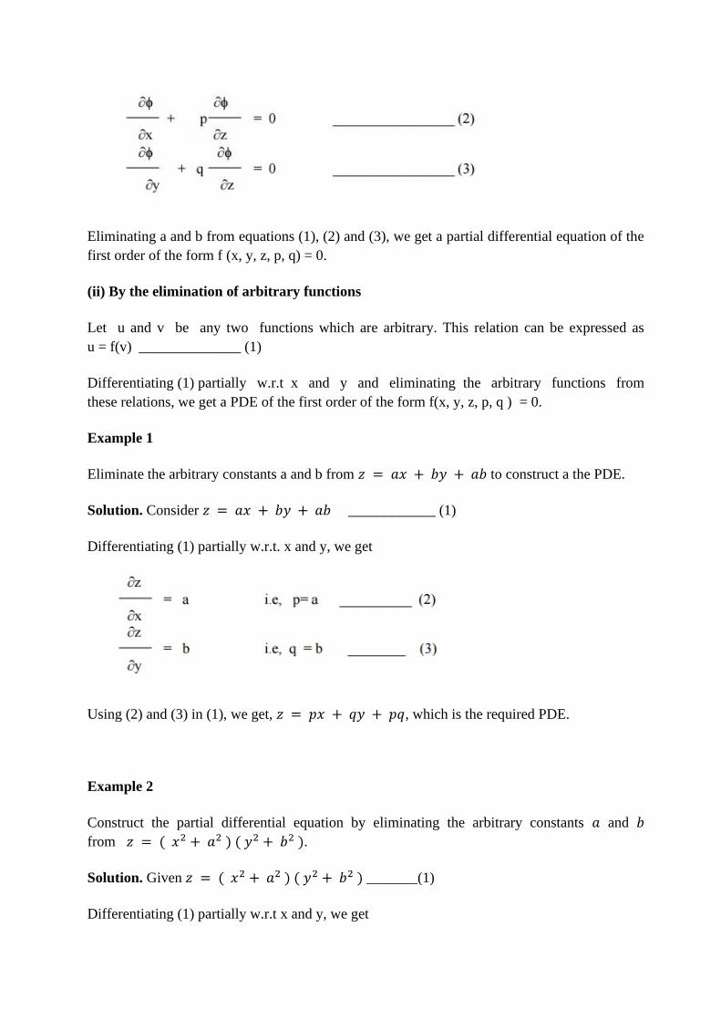
Eliminating a and b from equations (1), (2) and (3), we get a partial differential equation of the
first order of the form f (x, y, z, p, q) = 0.
(ii) By the elimination of arbitrary functions
Let u and v be any two functions which are arbitrary. This relation can be expressed as
u = f(v) ______________ (1)
Differentiating (1) partially w.r.t x and y and eliminating the arbitrary functions from
these relations, we get a PDE of the first order of the form f(x, y, z, p, q ) = 0.
Example 1
Eliminate the arbitrary constants a and b from 𝑧 = 𝑎𝑥 + 𝑏𝑦 + 𝑎𝑏 to construct a the PDE.
Solution. Consider 𝑧 = 𝑎𝑥 + 𝑏𝑦 + 𝑎𝑏 ____________ (1)
Differentiating (1) partially w.r.t. x and y, we get
Using (2) and (3) in (1), we get, 𝑧 = 𝑝𝑥 + 𝑞𝑦 + 𝑝𝑞, which is the required PDE.
Example 2
Construct the partial differential equation by eliminating the arbitrary constants 𝑎 and 𝑏
from 𝑧 = ( 𝑥2 + 𝑎2 ) ( 𝑦2 + 𝑏2 ).
Solution. Given 𝑧 = ( 𝑥2 + 𝑎2 ) ( 𝑦2 + 𝑏2 ) _______(1)
Differentiating (1) partially w.r.t x and y, we get

𝑝 = 2𝑥 (𝑦2 + 𝑏2 )
𝑞 = 2𝑦 (𝑥2 + 𝑎2 )
Substituting the values of p and q in (1), we get, 4𝑥𝑦𝑧 = 𝑝𝑞, which is the PDE.
Example 3
Find the partial differential equation of the family of spheres of radius one whose centre lie on
the 𝑥𝑦 − plane.
Solution.
The equation of the sphere is given by ( 𝑥 – 𝑎 )2 + ( 𝑦 – 𝑏 )2 + 𝑧2 = 1 _______ (1)
Differentiating (1) partially w.r.t x & y, we get, 2(𝑥 − 𝑎) + 2𝑧𝑝 = 0 and
2(𝑦 − 𝑏) + 2𝑧𝑞 = 0.
From these equations we obtain
𝑥 − 𝑎 = −𝑧𝑝 _________ (2)
𝑦 − 𝑏 = −𝑧𝑞 _________ (3)
Put (2) and (3) in (1), we get, 𝑧2𝑝2 + 𝑧2𝑞2 + 𝑧2 = 1 or 𝑧2(𝑝2 + 𝑞2 + 1)2 = 1
Example 4
Eliminate the arbitrary constants a, b and c from
and form the partial differential equation.

Solution.
Therefore, 𝑥𝑝2 − 𝑧𝑝 + 𝑥𝑧𝑟 = 0 is the required PDE.

Example 5
Example 6
Form the partial differential equation by eliminating the arbitrary function f
from 𝑧 = 𝑒𝑦 𝑓 (𝑥 + 𝑦)
Solution. Consider 𝑧 = 𝑒𝑦 𝑓 (𝑥 + 𝑦) ___________(1)
Differentiating (1) partially w.r.t x & y, we get
𝑝 = 𝑒𝑦 𝑓′(𝑥 + 𝑦)
𝑞 = 𝑒𝑦 𝑓′(𝑥 + 𝑦) + 𝑓(𝑥 + 𝑦). 𝑒𝑦
Hence, we have, 𝑞 = 𝑝 + 𝑧, which is the required PDE.
Example 7
Obtain the partial differential equation by eliminating f from the equation
𝑧 = (𝑥 + 𝑦)𝑓(𝑥2 − 𝑦2).
Solution.
Let us now consider the equation 𝑧 = (𝑥 + 𝑦)𝑓(𝑥2 − 𝑦2) _____________ (1)
Differentiating (1) partially w.r.t x & y, we get
𝑝 = (𝑥 + 𝑦)𝑓′(𝑥2 − 𝑦2). 2𝑥 + 𝑓(𝑥2 − 𝑦2)
𝑦 = (𝑥 + 𝑦)𝑓′(𝑥2 − 𝑦2). (−2𝑦) + 𝑓(𝑥2 − 𝑦2)

𝑝𝑦 − 𝑦𝑓(𝑥2 − 𝑦2) = −𝑞𝑥 + 𝑥𝑓(𝑥2 − 𝑦2)
𝑝𝑦 + 𝑞𝑥 = (𝑥 + 𝑦)𝑓(𝑥2 − 𝑦2)
Therefore, we have by (1), 𝑝𝑦 + 𝑞𝑥 = 𝑧, which is the required PDE.
Exercises:
3 Solutions of a Partial Differential Equation
A solution or integral of a partial differential equation is a relation connecting the
dependent and the independent variables which satisfies the given differential equation. A partial
differential equation can result both from elimination of arbitrary constants and from elimination
of arbitrary functions. But there is a basic difference in the two forms of solutions. A solution
containing as many arbitrary constants as there are independent variables is called a complete
integral. Here, the partial differential equations contain only two independent variables so that
the complete integral will include two constants. The solution obtained by giving particular
values to the arbitrary constants in a complete integral is called a particular integral.
Singular Integral
Let f (x,y,z,p,q) = 0 ________ (1)
be the partial differential equation whose complete integral is
f (x,y,z,a,b) = 0 ________(2)
where a and b are arbitrary constants.
Differentiating (2) partially w.r.t. a and b, we obtain

The eliminant of a and b from the equations (2), (3) and (4), when it exists, is called the singular
integral of (1).
General Integral
In the complete integral (2), put b = F(a), we get
f (x,y,z,a, F(a) ) = 0 ---------- (5)
Differentiating (2), partially w.r.t. a, we get
The eliminant of a between (5) and (6), if it exists, is called the general integral of (1).
4 Lagrange’s Linear Equation
Equations of the form Pp + Qq = R ________ (1), where P, Q and R are functions of
x, y, z, are known as Lagrange equations. To solve this equation, let us consider the
equations u = a and v = b, where a, b are constants and u, v are functions of x, y, z.
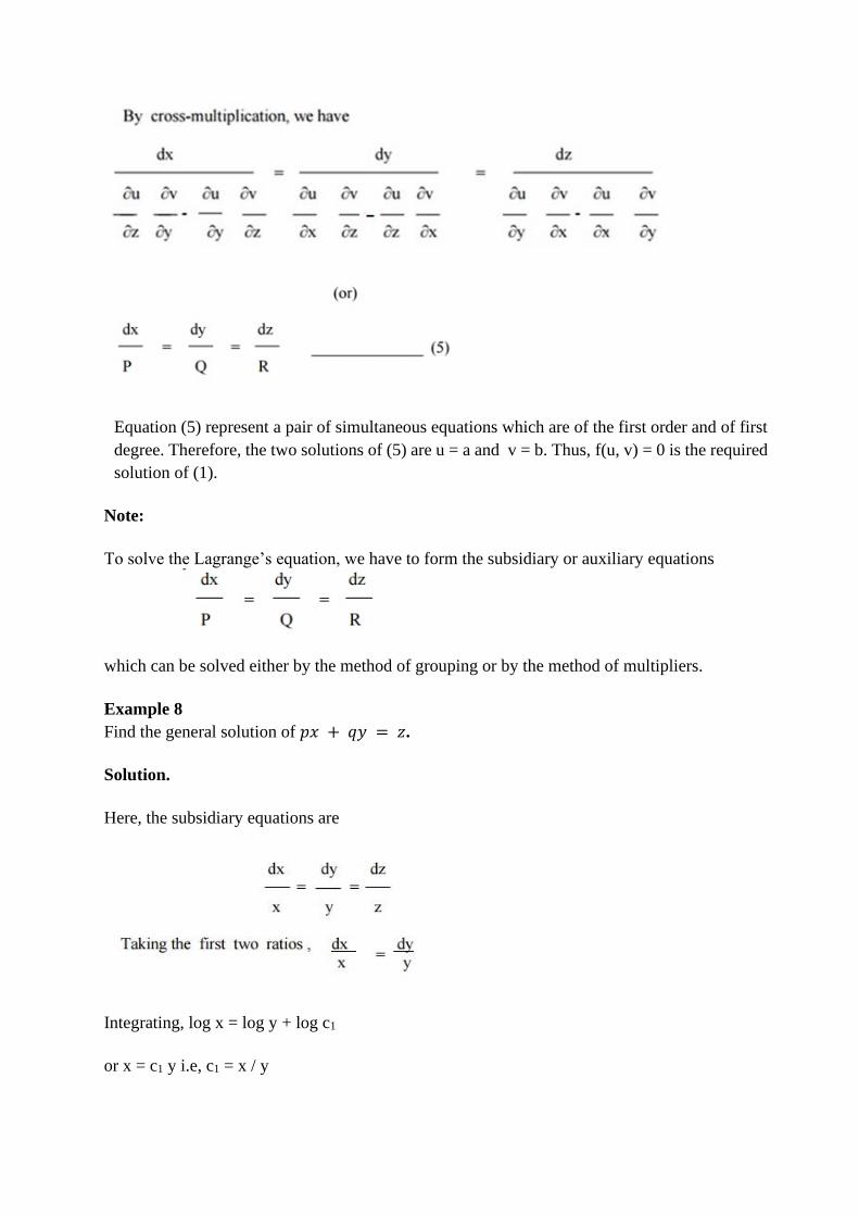
Equation (5) represent a pair of simultaneous equations which are of the first order and of first
degree. Therefore, the two solutions of (5) are u = a and v = b. Thus, f(u, v) = 0 is the required
solution of (1).
Note:
To solve the Lagrange’s equation, we have to form the subsidiary or auxiliary equations
which can be solved either by the method of grouping or by the method of multipliers.
Example 8
Find the general solution of 𝑝𝑥 + 𝑞𝑦 = 𝑧.
Solution.
Here, the subsidiary equations are
Integrating, log x = log y + log c1
or x = c1 y i.e, c1 = x / y

From the last two ratios,
Integrating, log y = log z + log c2
or y = c2 z
i.e, c2 = y / z
Hence the required general solution is Φ(x/y, y/z) = 0.
Example 9
Solve p tan x + q tan y = tan z
Solution.
The subsidiary equations are

Hence the required general solution is
.
Example 10
Solve (𝑦 − 𝑧) 𝑝 + (𝑧 − 𝑥) 𝑞 = 𝑥 − 𝑦.
Solution.
Here the subsidiary equations are

Example 11
Find the general solution of (𝑚𝑧 − 𝑛𝑦) 𝑝 + (𝑛𝑥 − 𝑙𝑧)𝑞 = 𝑙𝑦 − 𝑚𝑥.
Solution.


References
1. Narayanan, T.K. Manichavasagam Pillai, Calculus, Vol. I, S. Viswanathan Printers Pvt.
Limited, 2007.
2. Phoolan Prasad, Renuka Ravindran, Partial Differential Equations, John Wiley and Sons,
Inc., New York, 1984.

UNIT – IV – Ordinary and Partial Differential Equations – SMTA1305

UNIT – IV
Partial Differential Equations (Contd…)
1 Some Special Types of Equations which can be Solved Easily by Methods other than the
General Methods
The first order partial differential equation can be written as f(x, y, z, p, q) = 0, where 𝑝 =𝑑𝑧
𝑑𝑥 and
𝑞 =𝑑𝑧
𝑑𝑦. In this section, we shall solve some standard forms of equations by special methods.
Type I: f (p, q) = 0. (Equations containing p and q only).
Suppose that z = ax + by +c is a solution of the equation f(p, q) = 0,
where f (a, b) = 0.
Solving this for b, we get b = F (a).
Hence the complete integral is z = ax + F(a) y + c _________(1)
To find the singular integral, differentiate (1) w.r.t. a, we get, 0 = x + yF'(a)_____(2)
Now, the singular integral is obtained by eliminating a and c from (1) and (2), we get 0 = 1.
The last equation being absurd, the singular integral does not exist in this case.
To obtain the general integral, let us take c = F(a).
Then, z = ax + F(a) y + F(a) _________ (2)
Differentiating (2) partially w.r.t. a, we get
0 = x + F'(a). y + F '(a) _______ (3)
Eliminating a from (2) and (3), we get the general integral.
Example 1
Solve 𝑝𝑞 = 2
Solution.
The given equation is of the form f (p, q) = 0
The solution is z = ax + by +c, where ab = 2.

Solving, b = 2/a.
The complete integral is z = ax + 2/a y + c ---------- (1)
Differentiating (1) partially w.r.t c, we have, 0 = 1, which is absurd. Hence, there is no
singular integral. To find the general integral, put c = (a) in (1), we get, z = ax + 2/a y + F (a)
Differentiating partially w.r.t. a, we get,
0 = x – 2/ a2 y + F’(a)
Eliminating a between these equations, gives the general integral.
Example 2
Solve pq + p +q = 0
Solution.
The given equation is of the form f (p, q) = 0.
The solution is z = ax + by +c, where ab + a + b = 0.
Solving, we get
Differentiating (1) partially w.r.t. c, we get, 0 = 1.
The above equation being absurd, there is no singular integral for the given partial differential
equation.
To find the general integral, put c = F (a) in (1), we have

Differentiating (2) partially w.r.t a, we get
Eliminate a from (2) and (3) gives the general integral.
Example 3
Solve 𝑝2 + 𝑞2 = 𝑛𝑝𝑞.
Solution.
The solution of this equation is z = ax + by + c, where 𝑎2 + 𝑏2 = 𝑛𝑎𝑏.
Solving, we get,
Differentiating (1) partially w.r.t c, we get 0 = 1, which is absurd. Therefore, there is no singular
integral for the given equation.
To find the general integral, put C = F (a), we get
The eliminant of a between these equations gives the general integral.

Type II: Equations of the form f (x,p,q) = 0, f (y,p,q) = 0 and f (z,p,q) = 0. (One of the
variables x, y and z occurs explicitly)
(i) Let us consider the equation f (x,p,q) = 0.
Since z is a function of x and y, we have
or 𝑑𝑧 = 𝑝𝑑𝑥 + 𝑞𝑑𝑦
Assume that 𝑞 = 𝑎.
Then the given equation takes the form 𝑓 (𝑥, 𝑝, 𝑎 ) = 0.
Solving, we get p = F(x, a). Therefore, dz = F(x, a) dx + a dy.
(ii) Let us consider the equation f(y, p, q) = 0. Assume that p = a.
Then the equation becomes f (y, a, q) = 0 Solving, we get q = F (y, a).
Therefore, dz = adx + F(y,a) dy.
Integrating, z = ax + F(y,a) dy + b, which is a complete Integral.
(iii) Let us consider the equation f(z, p, q) = 0.
Assume that q = ap.
Then the equation becomes f (z, p, ap) = 0
Solving, we get p = F(z,a). Hence dz = F(z,a) dx + a F(z, a) dy.

Example 4
Solve q = xp + p2
Solution.
Given q = xp + p2 -------------(1)
This is of the form f (x, p, q) = 0.
Put q = a in (1), we get
a = xp + p2
i.e, p2 + xp – a = 0.
Therefore,
Thus,
Example 5
Solve q = y p2
Solution.
This is of the form f (y, p, q) = 0
Then, put p = a.

Therefore, the given equation becomes q = a2y.
Since dz = pdx + qdy, we have
dz = adx + a2y dy
Integrating, we get z = ax + (a2 y2/2) + b
Example 6
Solve 9 (p2 z + q2) = 4
Solution.
This is of the form f (z, p, q) = 0
Then, putting q = ap, the given equation becomes 9 (p2z + a2p2) = 4.
or (z + a2)3/2 = x + ay + b.

Type III: f1(x, p) = f2 (y, q). ie, equations in which ‘z’ is absent and the variables are
separable.
Let us assume as a trivial solution that f(x,p) = g(y,q) = a (say).
Solving for p and q, we get p = F(x, a) and q = G(y, a).
Hence dz = pdx + qdy = F(x, a) dx + G(y, a) dy
Therefore, z = òF(x, a) dx + òG(y, a) dy + b , which is the complete integral of the given equation
containing two constants a and b. The singular and general integrals are found in the usual way.
Example 7
Solve pq = xy
Solution.
The given equation can be written as

Example 8
Solve p2 + q2 = x2 + y2
Solution.
The given equation can be written as p2 – = y2 –q2 = a2 (say)
p2 – x2 = a2 implies p = √𝑥2 + 𝑎2
and y2 – q2 = a2 implies q = √𝑦2 − 𝑎2
But 𝑑𝑧 = 𝑝𝑑𝑥 + 𝑞𝑑𝑦
Type IV (Clairaut’s) form
Equation of the type z = px + qy + f (p,q) ------(1) is known as Clairaut’s form.
Differentiating (1) partially w.r.t x and y, we get p = a and q = b.
Therefore, the complete integral is given by
z = ax + by + f (a,b).
Example 9
Solve z = px + qy +pq
Solution.
The given equation is in Clairaut’s form
Putting p = a and q = b, we have ,
z = ax + by + ab -------- (1)
which is the complete integral.

To find the singular integral, differentiating (1) partially w.r.t a and b, we get
0 = x + b
0 = y + a
Therefore, we have, a = -y and b= -x.
Substituting the values of a & b in (1), we get, z = -xy –xy + xy
or z + xy = 0, which is the singular integral.
To get the general integral, put b = F(a) in (1).
Then z = ax + F(a)y + a F(a) ---------- (2)
Differentiating (2) partially w.r.t a, we have
0 = x + F'(a) y + aF'(a) + F(a) ---------- (3)
Eliminating a between (2) and (3), we get the general integral.
Example 10
Find the complete and singular solutions of


2 EQUATIONS REDUCIBLE TO THE STANDARD FORMS
Sometimes, it is possible to have non – linear partial differential equations of the first
order which do not belong to any of the four standard forms discussed earlier. By changing the
variables suitably, we will reduce them into any one of the four standard forms.
Type (I): Equations of the form F(xm p, ynq) = 0 (or) F (z, xmp, ynq) = 0.
Case(i): If m and n are not equal to 1 then put x1-m = X and y1-n = Y.
Hence, the given equation takes the form F(P, Q) = 0 (or) F(z, P, Q) = 0.
Case(ii) : If m = 1 and n = 1, then put log x = X and log y = Y.
Similarly, yq = Q
Example 11
Solve x4p2 + y2zq = 2z2

Solution.
The given equation can be expressed as (x2p)2 + (y2q)z = 2z2
Here m = 2, n = 2
Put X = x1-m = x -1 and Y = y 1-n = y -1.
We have xmp = (1- m) P and ynq = (1- n)Q
i.e, x2p = -P and y2q = -Q.
Hence the given equation becomes
P2 – Qz = 2z2 ----------(1)
This equation is of the form f (z, P, Q) = 0.
Let us take Q = aP.
Then equation (1) reduces to
P2 –aPz =2z2

Example 12
Solve x2p2 + y2q2 = z2
Solution.
The given equation can be written as (xp)2 + (yq)2 = z2
Here m = 1, n = 1.
Put X = log x and Y = log y.
Then xp = P and yq = Q.
Hence the given equation becomes
P2 + Q2 = z2 ------------- (1)
This equation is of the form F(z, P, Q) = 0.
Therefore, let us assume that Q = aP.
Now, equation (1) becomes,
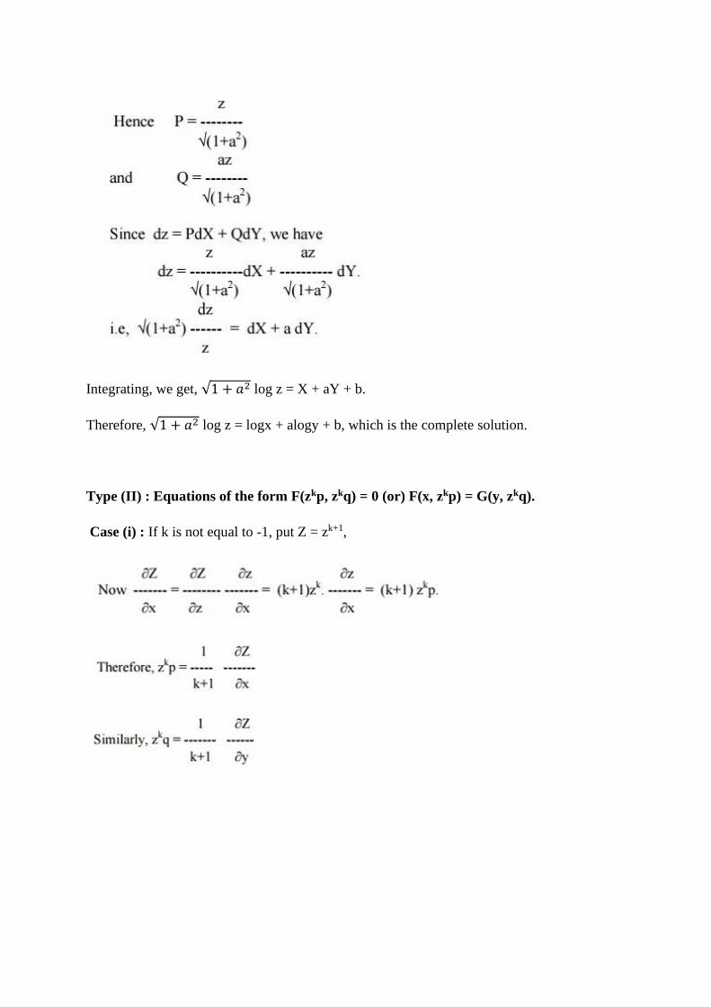
Integrating, we get, √1 + 𝑎2 log z = X + aY + b.
Therefore, √1 + 𝑎2 log z = logx + alogy + b, which is the complete solution.
Type (II) : Equations of the form F(zkp, zkq) = 0 (or) F(x, zkp) = G(y, zkq).
Case (i) : If k is not equal to -1, put Z = zk+1,

Example 13
Solve z4q2 –z2p = 1
Solution.
The given equation can also be written as (z2q)2 –(z2p) =1
Here k = 2. Putting Z = z k+1 = z3, we get
i.e, Q2 – 3P – 9 = 0, which is of the form F(P, Q) = 0.
Hence its solution is z = ax + by + c, where b2 – 3a – 9 = 0.
Solving for b, we get, b = ± √3𝑎 + 9
Hence the complete solution is Z = ax + √3𝑎 + 9 y + c
or z3 = ax + √3𝑎 + 9 y + c

3 Charpit’s Method
This is a general method to solve the most general non-linear PDE 𝑓(𝑥, 𝑦, 𝑧, 𝑝, 𝑞) = 0____(1) of
order one involving two independent variables. To solve (1), we solve the system of auxiliary
equations called Charpit’s equations.
𝑑𝑝
𝑓𝑥+𝑝𝑓𝑧=
𝑑𝑞
𝑓𝑦+𝑞𝑓𝑧=
𝑑𝑧
−𝑝𝑓𝑝−𝑞𝑓𝑞=
𝑑𝑥
−𝑓𝑝=
𝑑𝑦
−𝑓𝑞=
𝑑𝑓
0 _____(2).
Working rule of Charpit’s Method:
Step 1: Transfer all the terms of the PDE to LHS and denote the entire expression by
𝑓(𝑥, 𝑦, 𝑧, 𝑝, 𝑞) = 0.
Step 2: Write down Charpit’s auxiliary equations.
Step 3: Find 𝑓𝑥, 𝑓𝑦, 𝑓𝑧, 𝑓𝑝 and 𝑓𝑞. Put them in Step 2 and simplify.
Step 4: Choose two fractions such that the resulting integral is a simplest relation involving 𝑝 or
𝑞 or both.
Step 5: Use Step 4 to find 𝑝 and 𝑞 and put 𝑝 and 𝑞 in the equation 𝑑𝑧 = 𝑝𝑑𝑥 + 𝑞𝑑𝑦, which
on integration gives the complete integral.
Example 14
Find the complete integral of the PDE 3𝑝2 = 𝑞 using Charpit’s method.
Solution.
Given 3𝑝2 = 𝑞.
⟹ 3𝑝2 − 𝑞 = 0_______(1)
⟹ 𝑓 = 3𝑝2 − 𝑞.
⟹ 𝑓𝑥 = 0, 𝑓𝑦 = 0, 𝑓𝑧 = 0, 𝑓𝑝 = 6𝑝 and 𝑓𝑞 = −1.
Charpit’s auxiliary equations are:
𝑑𝑝
𝑓𝑥+𝑝𝑓𝑧=
𝑑𝑞
𝑓𝑦+𝑞𝑓𝑧=
𝑑𝑧
−𝑝𝑓𝑝−𝑞𝑓𝑞=
𝑑𝑥
−𝑓𝑝=
𝑑𝑦
−𝑓𝑞 .
𝑑𝑝
0=
𝑑𝑞
0=
𝑑𝑧
−6𝑝2+𝑞=
𝑑𝑥
−6𝑝=
𝑑𝑦
1 .

Taking the first fraction, 𝑑𝑝
0= 𝑘.
⟹ 𝑑𝑝 = 0.
Integrating, 𝑝 = 𝑎.
Substituting 𝑝 = 𝑎 in (1), 3𝑎2 − 𝑞 = 0.
⟹ 𝑞 = 3𝑎2.
Substituting 𝑝 and 𝑞 in 𝑑𝑧 = 𝑝𝑑𝑥 + 𝑞𝑑𝑦, we get, 𝑑𝑧 = 𝑎𝑑𝑥 + 3𝑎2𝑑𝑦.
Integrating, 𝑧 = 𝑎𝑥 + 3𝑎2𝑦 + 𝑏 is the complete integral.
4 Jacobi’s Method
This method is used to solve non-linear first order PDE which involves three or more
independent variables. Consider a non-linear PDE of order one of the form:
𝑓(𝑥1, 𝑥2, 𝑥3, 𝑝1, 𝑝2, 𝑝3) = 0______(1)
involving three independent variables 𝑥1, 𝑥2, 𝑥3 where the dependent variable 𝑧 do not occur
except by its partial derivatives 𝑝1 =𝔡𝑧
𝔡𝑥1, 𝑝2 =
𝔡𝑧
𝔡𝑥2, 𝑝3 =
𝔡𝑧
𝔡𝑥3.
To solve (1), we solve the following auxiliary equations:
𝑑𝑝1
𝑓 𝑥1
=𝑑 𝑥1
−𝑓𝑝1
=𝑑𝑝2
𝑓 𝑥2
=𝑑𝑥2
−𝑓𝑝2
=𝑑𝑝3
𝑓 𝑥3
=𝑑𝑥3
−𝑓𝑝3
.
Working rule of Jacobi’s Method:
Step 1: Transfer all the terms of the PDE to LHS and denote the entire expression by
𝑓(𝑥1, 𝑥2, 𝑥3, 𝑝1, 𝑝2, 𝑝3) = 0 ___(1).
Step 2: Write down Jacobi’s auxiliary equations.
Step 3: Find 𝑓𝑥1, 𝑓𝑥2
, 𝑓𝑥3, 𝑓𝑝1
, 𝑓𝑝2and 𝑓𝑝3
. Put them in Step 2 and simplify.
Step 4: Choose two fractions such that we obtain two additional equations as
𝐹1(𝑥1, 𝑥2, 𝑥3, 𝑝1, 𝑝2, 𝑝3) = 𝑐1_____(3) and 𝐹2(𝑥1, 𝑥2, 𝑥3, 𝑝1, 𝑝2, 𝑝3) = 𝑐2_____(4) where 𝑐1 and
𝑐2 are arbitrary constants. While obtaining (3) and (4), we try to select simple fractions from (2),
so that solution of equations (1), (3) and (4) may be as easy as possible.
Step 5: Verify that the relations (3) and (4) satisfy the condition ∑ (𝔡𝐹1
𝔡𝑥𝑖
𝔡𝐹2
𝔡𝑝𝑖−
𝔡𝐹2
𝔡𝑥𝑖
𝔡𝐹1
𝔡𝑝𝑖) = 03
𝑖=1 .

Step 6: If Step 5 is satisfied, then solve equations (1), (3) and (4) to find 𝑝1, 𝑝2, 𝑝3.
Step 7: Substitute 𝑝1, 𝑝2, 𝑝3 in the equation 𝑑𝑧 = 𝑝1𝑑𝑥1 + 𝑝2𝑑𝑥2 + 𝑝3𝑑𝑥3, which on
integration gives the complete integral.
Example 15
Find the complete integral of the PDE 𝑝13 + 𝑝2
2 + 𝑝3 = 1 using Jacobi’s method.
Solution.
Given 𝑝13 + 𝑝2
2 + 𝑝3 = 1.
⟹ 𝑝13 + 𝑝2
2 + 𝑝3 − 1 = 0_______(1)
𝑑𝑝1
𝑓 𝑥1
=𝑑 𝑥1
−𝑓𝑝1
=𝑑𝑝2
𝑓 𝑥2
=𝑑𝑥2
−𝑓𝑝2
=𝑑𝑝3
𝑓 𝑥3
=𝑑𝑥3
−𝑓𝑝3
.
𝑑𝑝1
0=
𝑑 𝑥1
− 3𝑝12 =
𝑑𝑝2
0=
𝑑𝑥2
−2𝑝2=
𝑑𝑝3
0=
𝑑𝑥3
−1 ______(2)
Taking the first and the third fractions of (2), we have 𝑑𝑝1 = 0 and 𝑑𝑝2 = 0 so that 𝑝1 = 𝑐1and
𝑝2 = 𝑐2, where 𝑐1 and 𝑐2 are arbitrary constants.
⟹ 𝑝1 = 𝑐1_____(3) and 𝑝2 = 𝑐2_____(4)
To verify whether ∑ (𝔡𝐹1
𝔡𝑥𝑖
𝔡𝐹2
𝔡𝑝𝑖−
𝔡𝐹2
𝔡𝑥𝑖
𝔡𝐹1
𝔡𝑝𝑖) = 03
𝑖=1 :
∑ (𝔡𝐹1
𝔡𝑥𝑖
𝔡𝐹2
𝔡𝑝𝑖−
𝔡𝐹2
𝔡𝑥𝑖
𝔡𝐹1
𝔡𝑝𝑖) = [(0)(0) − (1)(0)] + [(0)(1) − (0)(0)] + [(0)(0) − (0)(0)] = 03
𝑖=1 .
Since the equation is verified, we substitute 𝑝1 = 𝑐1and 𝑝2 = 𝑐2 in (1) to find 𝑝3.
⟹ 𝑝3 = 1 − 𝑐13 − 𝑐2
2.
Putting in 𝑑𝑧 = 𝑝1𝑑𝑥1 + 𝑝2𝑑𝑥2 + 𝑝3𝑑𝑥3 we get, 𝑧 = 𝑐1𝑥1 + 𝑐2𝑥2 + (1 − 𝑐13 − 𝑐2
2)𝑥3 +
𝑐3.
Reference
Dr. S. Sudha, Differential Equations & Integral Transforms, Emerald Publishers, 2002.

UNIT – V – Ordinary and Partial Differential Equations – SMTA1305

Unit V
Second and Higher Order Partial Differential Equations
This unit covers the following topics: Partial differential equations of second and higher order,
Classification of linear partial differential equations of second order, Homogeneous and
non-homogeneous equations with constant coefficients, Monge's methods.
1 Classification of linear partial differential equations of second order
The general second order linear PDE has the following form
𝐴𝑢𝑥𝑥 + 𝐵𝑢𝑥𝑦 + 𝐶𝑢𝑦𝑦 + 𝐷𝑢𝑥 + 𝐸𝑢𝑦 + 𝐹𝑢 = 𝐺,_______(1)
where the coefficients A, B, C, D, F and the free term G are in general functions of the
independent variables 𝑥, 𝑦, but do not depend on the unknown function 𝑢. The classification of
second order linear PDEs is given by the following:
The second order linear PDE (1) is called
(i) Hyperbolic, if 𝐵2 − 4𝐴𝐶 > 0
(ii) Parabolic, if 𝐵2 − 4𝐴𝐶 = 0
(ii) Elliptic, if 𝐵2 − 4𝐴𝐶 < 0
Example 1
Determine the regions in the 𝑥𝑦 −plane where the following equation is hyperbolic, parabolic,
or elliptic: 𝑢𝑥𝑥 + 𝑦𝑢𝑦𝑦 + 12𝑢𝑦.
Solution.
Given 𝑢𝑥𝑥 + 𝑦𝑢𝑦𝑦 + 12𝑢𝑦 .
The coefficients of the leading terms in this equation are: 𝐴 = 1, 𝐵 = 0, 𝐶 = 𝑦.
The discriminant is then 𝐵2 − 4𝐴𝐶 = −4𝑦.
Hence the equation is (i) hyperbolic when 𝑦 < 0, (ii) parabolic when 𝑦 = 0, and (iii) elliptic
when 𝑦 > 0.
Example 2
Classify the equation 𝑢𝑥𝑥 + 2𝑢𝑥𝑦 + 2𝑢𝑦𝑦 = 0.

Solution.
Here 𝐴 = 1, 𝐵 = 2, 𝐶 = −4.
The discriminant is then 𝐵2 − 4𝐴𝐶 = 4 − 4(1)(2) = −4 < 0.
Hence the equation is elliptic.
2 Homogeneous Partial Linear Differential Equations with constant Coefficients.
A homogeneous linear partial differential equation of the nth order is of the form
homogeneous because all its terms contain derivatives of the same order.
Equation (1) can be expressed as
As in the case of ordinary linear equations with constant coefficients the complete
solution of (1) consists of two parts, namely, the complementary function and the particular
integral.
The complementary function is the complete solution of f (D, D') z = 0-------(3), which must
contain n arbitrary functions as the degree of the polynomial f(D, D'). The particular integral is
the particular solution of equation (2).
Finding the complementary function
Let us now consider the equation f(D, D') z = F (x, y).
The auxiliary equation of (3) is obtained by replacing D by m and D' by 1.

Solving equation (4) for m, we get n roots. Depending upon the nature of the roots, the
Complementary function is written as given below:
Finding the particular Integral

Expand [f (D, D')]-1 in ascending powers of D or D' and operate on xm yn term by term.
Case (iv) : When F(x,y) is any function of x and y.
into partial fractions considering f (D,D') as a function of D alone.
Then operate each partial fraction on F(x,y) in such a way that
where c is replaced by y+mx after integration
Example 3
Solve (D3 –3D2D' + 4D'3) z = ex+2y
Solution.

The auxiliary equation is m3 – 3m2 + 4 = 0
The roots are : m = -1, 2, 2
Therefore, C.F. is f1(y-x) + f2 (y+ 2x) + xf3 (y+2x).
Hence, the solution is z = C.F. + P.I.
Example 4
Solve (D2 –4DD' +4 D'2) z = cos (x –2y)
Solution.
The auxiliary equation is m2 – 4m + 4 = 0
Solving, we get, m = 2, 2.
Therefore, C.F is f1(y+2x) + xf2(y+2x).

Example 5
Solve (D2 –2DD') z = x3y + e5x
Solution.
The auxiliary equation is m2 –2m = 0.
Solving, we get, m = 0, 2.
Hence, C.F. is f1 (y) + f2 (y+2x).

Example 6
Solution.
The auxiliary equation is m2 + m –6 = 0.
Therefore, m = –3, 2.
Hence, C.F. is f1(y-3x) + f2(y + 2x).

= (c + 3x) (–cosx) – (3) ( - sinx) – 2 sinx
= –y cosx + sinx
Hence the complete solution is
z = f1(y –3x) + f2(y + 2x) –y cosx + sinx
Example 7
Solve r – 4s + 4t = e 2x +y
Solution.
i.e, (D2 –4DD' + 4D' 2) z = e2x + y
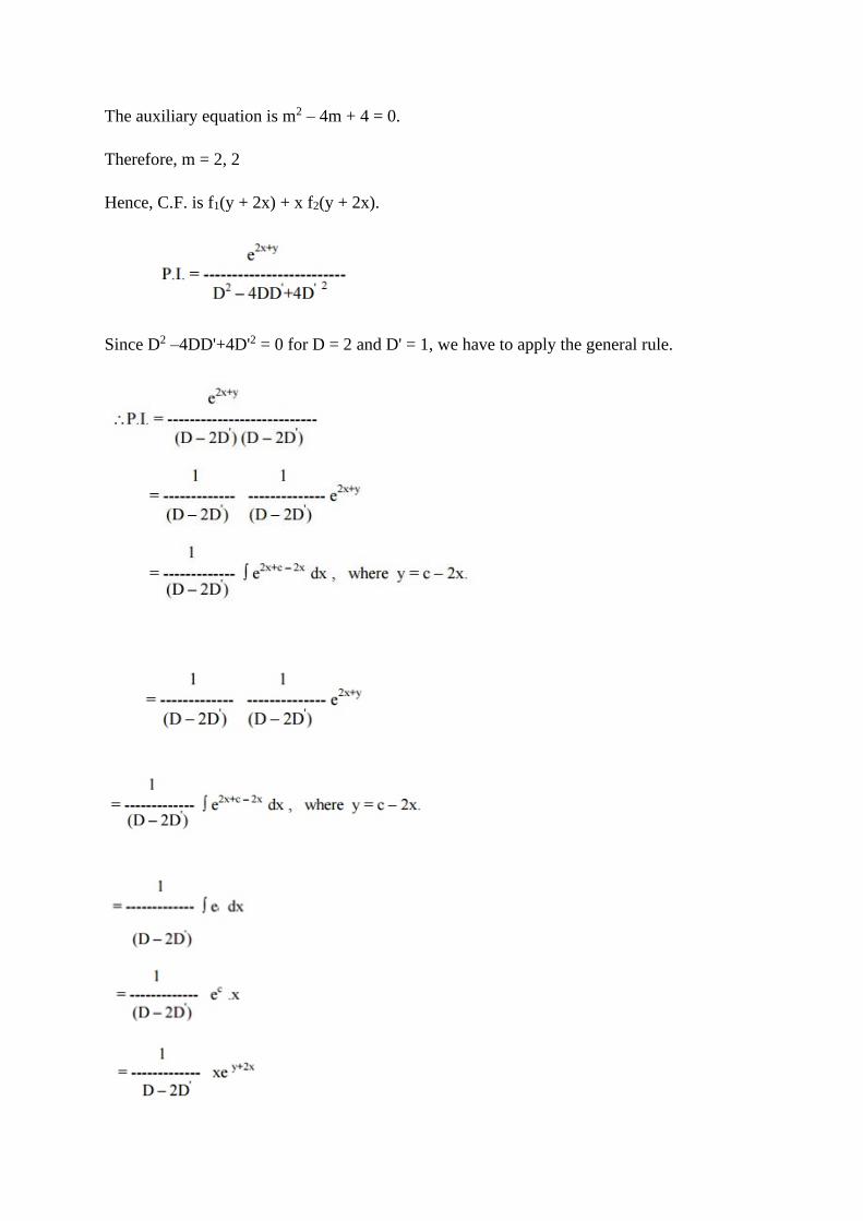
The auxiliary equation is m2 – 4m + 4 = 0.
Therefore, m = 2, 2
Hence, C.F. is f1(y + 2x) + x f2(y + 2x).
Since D2 –4DD'+4D'2 = 0 for D = 2 and D' = 1, we have to apply the general rule.

3 Non –Homogeneous Linear Equations
Let us consider the partial differential equation
f (D,D') z = F (x,y)------- (1)
If f (D,D') is not homogeneous, then (1) is a non–homogeneous linear partial differential
equation. Here also, the complete solution = C.F + P.I.
The methods for finding the Particular Integrals are the same as those for homogeneous linear
equations.
But for finding the C.F, we have to factorize f (D, D') into factors of the form D – mD' – c.
Consider now the equation (D –mD' –c) z = 0 ----------- (2).
This equation can be expressed as p –mq = cz ---------(3), which is in Lagrangian form.
The subsidiary equations are
The solutions of (4) are y + mx = a and z = becx.
Taking b = f (a), we get z = ecx f (y+mx) as the solution of (2).
Note:

1. If (D-m1D' –C1) (D –m2D'-C2) …… (D–mnDn'-Cn) z = 0 is the partial
differential equation, then its complete solution is
z = ec1
x f1(y +m1x) + ec2
x f2(y+m2x) + . . . . . + ecn
x fn(y+mnx).
2. In the case of repeated factors, the equation (D-mD' –Cn)z = 0 has a complete
solution z = ecx f1(y +mx) + x ecx f2(y+mx) + . . . . . +x n-1 ecx fn(y+mx).
Example 8
Solve (D-D'-1) (D-D' –2)z = e 2x –y
Solution.
Here, m1 = 1, m2 = 1, c1 = 1, c2 = 2.
Therefore, the C.F is ex f1 (y+x) + e2x f2 (y+x).
Example 9
Solve (D2 –DD' + D' –1) z = cos (x + 2y)
Solution.
The given equation can be rewritten as
(D-D'+1) (D-1) z = cos (x + 2y)
Here m1 = 1, m2 = 0, c1 = -1, c2 = 1.
Therefore, C.F. = e–x f1(y+x) + ex f2 (y)

Example 10
Solve [(D + D'–1) (D + 2D' –3)] z = ex+2y + 4 + 3x +6y
Solution.
Here m1 = –1, m2 = –2, c1 = 1, c2 = 3.
Hence the C.F is z = ex f1(y –x) + e3x f2(y –2x).

4 Monge’s Method
This method is used to solve non-linear second order PDE with the standard form
𝑅𝑟 + 𝑆𝑠 + 𝑇𝑡 = 𝑉___________(1)
Where R, S, T and V are functions of x, y, z, p and q.
Procedure to solve by Monge’s method:

Step1: Write the given PDE in the standard form and find R, S, T and V.
Step 2: The auxiliary equations are:
𝑅𝑑𝑝𝑑𝑦 + 𝑇𝑑𝑞𝑑𝑥 − 𝑉𝑑𝑥𝑑𝑦 = 0____________(2)
𝑅(𝑑𝑦)2 − 𝑆𝑑𝑥𝑑𝑦 + 𝑇(𝑑𝑥)2 = 0____________(3)
Step 3: First factorise equation (3) and get the factors in terms of 𝑑𝑥 and 𝑑𝑦.
Step 4: If these factors are equations (4) and (5), use each factor in (2) to get equations (6) and
(7).
Step 5: Obtain the values of p and q using equations (6) and (7).
Step 6: The general solution of (1) is 𝑑𝑧 = 𝑝𝑑𝑥 + 𝑞𝑑𝑦.
Example 11
Using Monge’s method, solve 𝑟2 = 𝑎𝑡.
Solution.
Given equation is 𝑟2 = 𝑎𝑡_____________(1)
Here 𝑅 = 1, 𝑆 = 0, 𝑇 = −𝑎2, 𝑉 = 0.
Monge’s auxiliary equations are:
𝑅𝑑𝑝𝑑𝑦 + 𝑇𝑑𝑞𝑑𝑥 − 𝑉𝑑𝑥𝑑𝑦 = 0____________(2)
𝑅(𝑑𝑦)2 − 𝑆𝑑𝑥𝑑𝑦 + 𝑇(𝑑𝑥)2 = 0____________(3)
From (3), we have, (𝑑𝑦)2 − 𝑎2(𝑑𝑥)2 = 0.
⟹ (𝑑𝑦 − 𝑎𝑑𝑥) = 0 and (𝑑𝑦 + 𝑎𝑑𝑥) = 0.
⟹ 𝑑𝑦 = 𝑎𝑑𝑥 and 𝑑𝑦 = −𝑎𝑑𝑥.
Integrating both the equations, we get,
⟹ 𝑦 = 𝑎𝑥 + 𝑐1 and 𝑦 = −𝑎𝑥 + 𝑐2.
⟹ 𝑦 − 𝑎𝑥 = 𝑐1 ______(4) and 𝑦 + 𝑎𝑥 = 𝑐2_____(5)
Case(i) Put (4) in (2).
⟹ 𝑑𝑝(𝑎𝑑𝑥) − 𝑎2𝑑𝑞𝑑𝑥 = 0.
⟹ 𝑑𝑝 − 𝑎𝑑𝑞 = 0.
Integrating, we get,
⟹ 𝑝 − 𝑎𝑞 = 𝜑1(𝑦 − 𝑎𝑥)_________(6) [using equation(4)]
Case(ii) Put (5) in (2).
⟹ 𝑑𝑝(𝑎𝑑𝑥) + 𝑎2𝑑𝑞𝑑𝑥 = 0.
⟹ 𝑑𝑝 + 𝑎𝑑𝑞 = 0.
Integrating, we get,
⟹ 𝑝 + 𝑎𝑞 = 𝜑2(𝑦 + 𝑎𝑥)_________(7) [using equation(5)]
(6) + (7) ⟹ 2𝑝 = 𝜑1(𝑦 − 𝑎𝑥) + 𝜑2(𝑦 + 𝑎𝑥).
⟹ 𝑝 =1
2[𝜑1(𝑦 − 𝑎𝑥) + 𝜑2(𝑦 + 𝑎𝑥)].
(7) − (6) ⟹ 2𝑎𝑞 = 𝜑2(𝑦 + 𝑎𝑥) − 𝜑1(𝑦 − 𝑎𝑥).
⟹ 𝑞 =1
2𝑎[𝜑2(𝑦 + 𝑎𝑥) − 𝜑1(𝑦 − 𝑎𝑥)].
The general solution of (1) is 𝑑𝑧 = 𝑝𝑑𝑥 + 𝑞𝑑𝑦.
Substituting 𝑝 and 𝑞 in 𝑑𝑧 = 𝑝𝑑𝑥 + 𝑞𝑑𝑦, we get,
𝑑𝑧 =1
2[𝜑1(𝑦 − 𝑎𝑥) + 𝜑2(𝑦 + 𝑎𝑥)]𝑑𝑥 +
1
2𝑎[𝜑2(𝑦 + 𝑎𝑥) − 𝜑1(𝑦 − 𝑎𝑥)]𝑑𝑦.
Simplifying and integrating we get,
𝑧 = 𝜓1(𝑦 − 𝑎𝑥) + 𝜓2(𝑦 + 𝑎𝑥)].

The arbitrary constant of integration may be considered as absorbed in either of the functions
𝜓1(𝑦 − 𝑎𝑥) or 𝜓2(𝑦 + 𝑎𝑥).
Therefore, the complete integral is 𝑧 = 𝜓1(𝑦 − 𝑎𝑥) + 𝜓2(𝑦 + 𝑎𝑥)] where 𝜓1 and 𝜓2 are
arbitrary functions.
References
1. Phoolan Prasad, Renuka Ravindran, Partial Differential Equations, John Wiley and Sons,
Inc., New York, 1984.