Scheduling of Flexible Job Shop Problem in DynamicEnvironments

Mariana Bayão Horta Mesquita da Cunha

Thesis to obtain the Master of Science Degree in

Mechanical Engineering

Supervisors: Prof. João Miguel da Costa Sousa

Prof. Susana Margarida da Silva Vieira

Examination Committee

Chairperson: Prof. Paulo Jorge Coelho Ramalho Oliveira

Supervisor: Prof. João Miguel da Costa Sousa

Members of the Committee: Prof. Carlos Augusto Santos Silva

Prof. João Manuel Gouveia de Figueiredo

November, 2017

Acknowledgements

To Professor João Sousa and Susana Vieira, for all the guidance throughout the thesis and for pressuring me

when I needed.

To my family for all the support during this �ve years. A special thank you to my father for endless work

revisions, my mother for all the empathy and understanding, and last but not least, Miguel for never refusing

to let me take his computer.

To Diogo, �ve years always by my side.

To FST Lisbon an enormous challenge with great friends.

To the 2012 gang, specially to Raquel.

i

Resumo

A capacidade de recolher, armazenar e trabalhar dados nunca foi tão grande. Este novo paradigma está

a mudar a indústria. Com as decisões certas, suportadas por dados, a possibilidade de diminuir custos e

aumentar a e�ciência das fábricas podem vir a mudar todo a estrutura das empresas. Dentro da Indústria

4.0, o escalonamento em ambiente dinâmico é uma das grandes oportunidades. Com conhecimento do estado

da fábrica, o escalonamento pode passar a ser feito em tempo real, optimizando não só o comportamento

esperado como adaptando-o conforme o estado actual.

Dois métodos de planeamento foram usados: Programação Linear com Inteiros, MILP , e um algoritmo

genético com procura local, hGAJobs. O MILP proposto não conseguiu resolver problemas com 10 ordens,

10 operações cada e 10 máquinas. Ainda assim, conseguiu resolver problemas de menores dimensões. O

algoritmo genético proposto, hGAJobS, combina diferentes métodos de geração de população inicial e de

criação de futuras gerações, com um sistema de codi�cação que garante soluções na região exequível. O

algoritmo proposto junta ainda um método de procura local. O hGAJobs foi aplicado em datasets de

produção �exível e obteve uma boa performance em comparação com outros algoritmos genéticos existentes.

Para reagir a situações dinâmicas dois algoritmos multi-agentes inspirados em formigas são apresentados.

O primeiro com uma arquitectura autónoma, AABS. Devido à miopia associada a arquitecturas autónomas,

uma nova abordagem sob uma arquitectura mediada é proposta, MABS. Após testes do algoritmo AABS

em problemas conhecidos, este é comparado com o algoritmo MABS.

Keywords: Produção �exível; Ambiente dinâmico; Programação Linear com Inteiros; Algoritmo

genético; Procura Local; Sistemas multi-agentes;

ii

Abstract

Data collection is reaching unprecedented high levels and the ability to analyse it is turning industries into

digital. With the right decisions supported by data, cost savings and plant e�ciency have the potential to

change the whole business structures. Within Industry 4.0, scheduling in dynamic environments is one of the

major opportunities. Presently, real-time knowledge of the plant scheduling can be done as online activity,

optimizing not only the expected process but adapting as well to real unforeseen events. In this thesis tools

are provided to both plan in a static predicted environment and to react in case of disturbance.

Two planning techniques were implemented: a deterministic mixed integer linear programming model,

MILP , and a genetic algorithm with a variable neighbourhood search, hGAJobS. The proposed MILP

algorithm was unable to solve instances with 10 jobs, consisting of 10 operations each, and 10 machines.

However, it was able to successfully solve less complex instances. The proposed genetic algorithm, hGAJobs,

combines di�erent initial population creation and o�spring generation methods, with a coding system that

only allows feasible solutions. Moreover, to this genetic algorithm a variable neighbourhood search is added.

hGAJobs was applied to various Flexible Job Shop problem performing well in comparison to other genetic

algorithms in the literature.

To respond in a dynamic environment two ant inspired multi-agent algorithms are proposed. The �rst

is an autonomous architecture, AABS. Because of the myopia associated with autonomous architectures, a

novel approach is proposed in a mediator architecture, MABS.

Keywords: Flexible job shop; Dynamic environment; Mixed integer linear programming; Genetic

algorithm; Variable neighbourhood search; Multi-agent based systems;

iii

Contents

Resumo ii

Abstract iii

Contents iv

List of Tables vi

List of Figures vii

1 Introduction 1

1.1 Scheduling in Manufacturing Systems . . . . . . . . . . . . . . . . . . . . . . . . . . . 2

1.1.1 Scheduling Technologies . . . . . . . . . . . . . . . . . . . . . . . . . . . . . . . . 5

1.2 Contributions . . . . . . . . . . . . . . . . . . . . . . . . . . . . . . . . . . . . . . . . . . . 10

1.3 Thesis Outline . . . . . . . . . . . . . . . . . . . . . . . . . . . . . . . . . . . . . . . . . . . 10

2 The Flexible Job Shop Problem 12

2.1 Representation . . . . . . . . . . . . . . . . . . . . . . . . . . . . . . . . . . . . . . . . . . 13

2.2 Performance Measures and Objectives . . . . . . . . . . . . . . . . . . . . . . . . . . 15

3 Static Scheduling 17

3.1 Mixed Integer Linear Programming . . . . . . . . . . . . . . . . . . . . . . . . . . . . . 17

3.2 Genetic Algorithm . . . . . . . . . . . . . . . . . . . . . . . . . . . . . . . . . . . . . . . . 19

3.2.1 Coding . . . . . . . . . . . . . . . . . . . . . . . . . . . . . . . . . . . . . . . . . . . . 20

3.2.2 Initial Population . . . . . . . . . . . . . . . . . . . . . . . . . . . . . . . . . . . . 22

3.2.3 Mutation Operators . . . . . . . . . . . . . . . . . . . . . . . . . . . . . . . . . . . 26

3.2.4 Crossover Operators . . . . . . . . . . . . . . . . . . . . . . . . . . . . . . . . . . 26

3.2.5 Variable Neighbourhood Search . . . . . . . . . . . . . . . . . . . . . . . . . . . 27

4 Dynamic Scheduling 30

4.1 Autonomous Ant Based System . . . . . . . . . . . . . . . . . . . . . . . . . . . . . . . . 30

4.1.1 Agent Coordination . . . . . . . . . . . . . . . . . . . . . . . . . . . . . . . . . . . 31

4.2 Mediator Ant Based System . . . . . . . . . . . . . . . . . . . . . . . . . . . . . . . . . . 36

5 Results and Discussion 39

5.1 MILP . . . . . . . . . . . . . . . . . . . . . . . . . . . . . . . . . . . . . . . . . . . . . . . . . 39

5.2 Genetic Algorithm . . . . . . . . . . . . . . . . . . . . . . . . . . . . . . . . . . . . . . . . 42

5.2.1 Initial Population Creation . . . . . . . . . . . . . . . . . . . . . . . . . . . . . . 42

iv

5.2.2 Population Size . . . . . . . . . . . . . . . . . . . . . . . . . . . . . . . . . . . . . . 43

5.2.3 Chosen Parameters . . . . . . . . . . . . . . . . . . . . . . . . . . . . . . . . . . . . . . 45

5.2.4 Results . . . . . . . . . . . . . . . . . . . . . . . . . . . . . . . . . . . . . . . . . . . . 46

5.3 Hybrid Genetic Algorithm . . . . . . . . . . . . . . . . . . . . . . . . . . . . . . . . . . . 47

5.4 Dynamic Testing . . . . . . . . . . . . . . . . . . . . . . . . . . . . . . . . . . . . . . . . . . 49

5.4.1 GM truck Painting . . . . . . . . . . . . . . . . . . . . . . . . . . . . . . . . . . . . 50

5.4.2 Flexible Plant Study-case . . . . . . . . . . . . . . . . . . . . . . . . . . . . . . . 54

6 Conclusions 61

6.1 Future Work . . . . . . . . . . . . . . . . . . . . . . . . . . . . . . . . . . . . . . . . . . . . 62

7 References 63

v

List of Tables

1 Processing time of each operation Oi in each machine M . . . . . . . . . . . . . . . . . . . . . 12

2 Parameters used in MILP formulation . . . . . . . . . . . . . . . . . . . . . . . . . . . . . . . 18

3 Variables used in MILP formulation . . . . . . . . . . . . . . . . . . . . . . . . . . . . . . . . 18

4 Assignment part of the chromosome . . . . . . . . . . . . . . . . . . . . . . . . . . . . . . . . 21

5 Sequencing part of the chromosome . . . . . . . . . . . . . . . . . . . . . . . . . . . . . . . . . 21

6 First steps and �nal result of the smallest processing time method for assignment illustrated

using table 1 . . . . . . . . . . . . . . . . . . . . . . . . . . . . . . . . . . . . . . . . . . . . . 23

7 First steps and �nal result of the reordering assignment method illustrated using table 1 . . . 25

8 Agent types and functions . . . . . . . . . . . . . . . . . . . . . . . . . . . . . . . . . . . . . . 31

9 Agent types and functions in the mediator architecture . . . . . . . . . . . . . . . . . . . . . . 36

10 Processing time of each operation Oi in each machine M . . . . . . . . . . . . . . . . . . . . . 37

11 Makespan obtained and best known Lower Bound (LB) using the MILP algorithm and the

GAJobs. . . . . . . . . . . . . . . . . . . . . . . . . . . . . . . . . . . . . . . . . . . . . . . . . 40

12 Brandimarte dataset instances characteristics. Lower and upper bounds correspond to makespan

(Cmax). . . . . . . . . . . . . . . . . . . . . . . . . . . . . . . . . . . . . . . . . . . . . . . . . 42

13 Population size for each test instance . . . . . . . . . . . . . . . . . . . . . . . . . . . . . . . . 45

14 Genetic algorithm parameters . . . . . . . . . . . . . . . . . . . . . . . . . . . . . . . . . . . . 46

15 Makespan, Cmax, for the Brandimarte dataset (* represents best known Lower Bound). . . . 47

16 Population size for each test instance using hGAJobS . . . . . . . . . . . . . . . . . . . . . . 48

17 Makespan, Cmax, for the Brandimarte dataset (* represents best known Lower Bound). . . . 49

18 Problem and AABS settings . . . . . . . . . . . . . . . . . . . . . . . . . . . . . . . . . . . . 53

19 Comparison of results for GM truck painting problem. Not very signi�cant setup penalty,

tsetup = 1min. Results for 100 simulations. . . . . . . . . . . . . . . . . . . . . . . . . . . . . 54

20 Comparison of results for GM truck painting problem. Very signi�cant setup penalty, tsetup =

10min. Results for 100 simulations. . . . . . . . . . . . . . . . . . . . . . . . . . . . . . . . . . 54

21 Part types routing, mean processing time and probability of arriving . . . . . . . . . . . . . . 55

vi

List of Figures

1 Scheme of the rescheduling framework used. The grey boxes represent the approach taken to

the problem. . . . . . . . . . . . . . . . . . . . . . . . . . . . . . . . . . . . . . . . . . . . . . 4

2 Example of a disjunctive graph. The full arcs correspond to conjunctive arcs, and dashed arcs

are the disjunctive arcs. . . . . . . . . . . . . . . . . . . . . . . . . . . . . . . . . . . . . . . . 13

3 Example of a disjunctive graph with a determined sequence. Arcs in bold correspond to the

critical path . . . . . . . . . . . . . . . . . . . . . . . . . . . . . . . . . . . . . . . . . . . . . . 15

4 Genetic Algorithm Process . . . . . . . . . . . . . . . . . . . . . . . . . . . . . . . . . . . . . 20

5 Gantt chart result of example chromosome assignment and sequence represented in table 4

and 5, respectively . . . . . . . . . . . . . . . . . . . . . . . . . . . . . . . . . . . . . . . . . . 22

6 Illustration of Precedence Preserving Shift mutation. The �rst operation of job 3 will take the

sequence's 5th position. . . . . . . . . . . . . . . . . . . . . . . . . . . . . . . . . . . . . . . . 26

7 Crossover Operators. . . . . . . . . . . . . . . . . . . . . . . . . . . . . . . . . . . . . . . . . . 27

8 Shop scheduling process . . . . . . . . . . . . . . . . . . . . . . . . . . . . . . . . . . . . . . . 31

9 Organizational methodology of an ant colony searching for food. . . . . . . . . . . . . . . . . 32

10 Multi-agent based systems mediator architecture . . . . . . . . . . . . . . . . . . . . . . . . . 37

11 Crossover Operators. . . . . . . . . . . . . . . . . . . . . . . . . . . . . . . . . . . . . . . . . . 38

12 Gantt chart and makespan for mt06s instance using MILP algorithm (Cmax = 55) . . . . . . 40

13 Gantt chart and makespan for mt03e instance using MILP algorithm (Cmax = 47) . . . . . . 41

14 Gantt chart and makespan for mt06e instance using MILP algorithm (Cmax = 55) . . . . . . 41

15 Initial population �tness value when varying the assignment and sequencing methods fractions. 44

16 Population size convergence analysis for the Mk10 dataset. . . . . . . . . . . . . . . . . . . . 45

17 Gantt chart and makespan for Mk01 with GAJobS (Cmax = 42) . . . . . . . . . . . . . . . . 48

18 Gantt chart and makespan for Mk01 with hGAJobS (Cmax = 40) . . . . . . . . . . . . . . . . 50

19 Schematics of the factory layout for the GM case . . . . . . . . . . . . . . . . . . . . . . . . . 51

20 Throughput varying according to the combination of heuristic weighting parameter,β, and

pheromone weighting parameter, α, in 1000 simulated minutes . . . . . . . . . . . . . . . . . 53

21 Schematics of the �exible plant layout . . . . . . . . . . . . . . . . . . . . . . . . . . . . . . . 55

22 Mean lateness results comparison between AABS and MABS algorithms when varying due

date tightness factor k. . . . . . . . . . . . . . . . . . . . . . . . . . . . . . . . . . . . . . . . . 57

23 Maximum lateness results comparison between AABS and MABS algorithms when varying

due date tightness factor k. . . . . . . . . . . . . . . . . . . . . . . . . . . . . . . . . . . . . . 57

24 Throughput per 8 time units results comparison between AABS andMABS algorithms when

varying due date tightness factor k. . . . . . . . . . . . . . . . . . . . . . . . . . . . . . . . . . 58

vii

25 Maximum queue length comparison between AABS andMABS algorithms when varying due

date tightness factor k. . . . . . . . . . . . . . . . . . . . . . . . . . . . . . . . . . . . . . . . . 60

viii

1 Introduction

Increasing data collection and storage together with new computational capabilities are leading to major

changes in the industry. Just as steam engine powered factories in the XIXth century, electri�cation enabled

mass production in the XXth century, and automation in the 70s were revolutionary in their time, now is

the rise of digital industry known as Industry 4.0. Sensors, machines, parts and information systems will

be connected forming cyberphysical systems. These systems will be able to analyse data, predict failures

and adapt to changes. Hence processes will be much faster, �exible and e�cient, producing high quality,

customized and on-time goods at lower costs [1, 2].

Industry 4.0 will enable companies to cut on costs and save time on both services and production, through

better planning and man-machine interfaces, better production control, raw material availability control,

inventory levels, and energy consumption. With the right decision making in place, customer and suppliers

relations can be signi�cantly improved.

The combination of these factors has opened opportunities for the chemical industry, namely the phar-

maceutical industry. The pharmaceutical industry has been su�ering from increasingly high R&D costs [3].

These costs have been mainly associated with the shifting paradigm forcing the industry to change from a

one-drug-�ts-all approach to ever more targeted drugs for small and speci�c patient and therapeutic groups.

To secure revenue, companies are pressured to diversify their product portfolio. Therefore, there is a big

opportunity to increase pro�t by cutting costs in the production and quality control phases, achieving higher

throughput rates, lower energy consumption and more e�ective and planned maintenance, while still main-

taining high quality levels. The large amount of data collected can be used to improve plants and make

better-informed decisions across the whole company business, with the potential to change value chains,

reach higher productivity and lead to more innovation. The application of Industry 4.0 principles to the

pharmaceutical industry is the now called Pharma 4.0, with the potential to overcome the industry's recent

challenges.

It is within Industry 4.0 scope, and more speci�cally Pharma 4.0, that the scheduling and rescheduling

problem arises. To improve plant productivity, and having data from demands and plant state, it is possible to

make planning decision to optimize future outcome, corresponding to either minimize costs and/or maximize

revenues. Furthermore, with a rescheduling strategy, not only the plan is optimized but it is updated according

to the evolving current plant situation.

In this chapter, a literature review on scheduling and rescheduling methods and policies will be presented.

The main research was focused on the �exible job shop problem, once it represents the problem in hands in

the pharmaceutical industry. The �exible job shop problem, a well known NP-hard problem, is an extension

of the classical job shop problem, where there is both job arrival and process �ow variability, as well as a

combination of machines able to preform the same operation. At the end of the chapter a guideline of the

thesis is given.

1

1.1 Scheduling in Manufacturing Systems

Scheduling may be broadly de�ned as the allocation of resources over a time period seeking to maximize or

minimize a performance indicator. It is a common concern in most economic domains, such as computer

engineering [4], ship scheduling [5], dispatching of short-term hydro power plants [6], micro-grid energy

management [7] or crude oil short term scheduling unloading [8]. Nevertheless, most research is regarding

manufacturing and production plants scheduling, since, due to the by the markets pressure, it is critical to

reduce costs and increase productivity.

Determining the best schedule can be a trivial task or a very complex problem, depending on the environ-

ment, process constraints and the performance indicator [9]. Particularizing to the manufacturing scheduling

problem one can �nd two main streams: the job shop problem, JSP; and the �exible job shop problem, FJSP.

The former represents one of the most di�cult problems, in which a set of operations, each one requiring

a single machine, which can process uninterruptedly one operation at a time and the machines are contin-

uously available, being a NP-Hard problem. The latter extends the former, in the way that operations are

allowed to be processed by a machine on a set of available ones. The main goal of the JSP is to sequence

the operations to maximize the performance measured by the chosen indicator. The FJSP introduces a new

decision dimension, since it demands not only the sequence of operations but also the machine allocation,

also referred as the job routes. Consequently, the JSP space of solutions is a subspace of the FJSP space of

solutions, SJSP ⊂ SFJSP . The work on [10] demonstrates the NP-hardness and combinatorial characteristics

of FJSP.

Manufacturing systems plants usually have an a priori plan for when activities should take place according

to a predetermined objective. Nonetheless, real world manufacturing systems are dynamic systems with

uncertainty which, typically, have two sources:

• Resource Related - machine breakdown, operator uncertain performance or illness, loading limits,

unavailability or tool breakdown, materials shortage or arrival delay, not compliant materials, etc.

• Jobs Related - last minute high priority jobs, jobs cancellation, due dates alteration, unexpected jobs

arrival, jobs processing time change, etc.

A dynamic environment prone to unpredictability and uncertainty, as the ones aforementioned, may result

in a poor manufacturing system performance of the previously scheduled activities. Inevitably, to reduce the

deviation from reality a new type of scheduling techniques has been created, known as dynamic scheduling

[11]. To account for real time events and to address its changes and minimize their e�ect on the shop �oor,

a great deal of e�ort has been spent on rescheduling, which is the process of updating an existing production

scheduling when facing disruptive events [12].

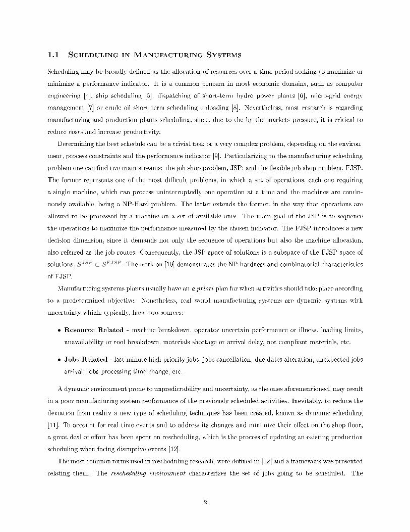
The most common terms used in rescheduling research, were de�ned in [12] and a framework was presented

relating them. The rescheduling environment characterizes the set of jobs going to be scheduled. The

2

rescheduling strategy represents the dynamic scheduling technologies categories. Finally, rescheduling policy

refers to rules or circumstances which determine when the reschedule shall take place.

In terms of rescheduling environment, it can be either static, when a �nite set of jobs is considered,

or dynamic, referring to an in�nite set of jobs or real-time events. A dynamic scheduling environment

can be divided in three cases. First, continuous manufacturing, where a machine or facility produces the

same/identical items in long runs [9]. Second, �ow shop facility, where all jobs �ow in the same fashion

through the facility although there might be uncertainty in job arrival time. And last, job shop case, where

a combination of job arrival uncertainty and process �ow variability may occur.

In [13], similarly to [12], research in dynamic scheduling is classi�ed under three categories according

to the scheduling strategy used, completely reactive, predictive-reactive and robust pro-active. Completely

reactive scheduling is a scheduling scheme where no schedule is generated in advance. Scheduling decisions

are made, when necessary, using information available at the moment. In this scheduling scheme dispatching

rules, such as Earliest Due Date or Shortest Processing Time [9, 14], and also pull mechanisms, Kaban cards

and CONWIP [15], are commonly used. This strategy relies on local decisions made in real time to respond

to machines that are free or new jobs arriving. Yet, there is room for improvement when considering a global

scheduling that considers all the shop over a time period, which when compared to local and myopic decisions

may signi�cantly increase the shop performance.

Predictive-reactive scheduling is the most common dynamic scheduling strategy [13]. It consists on a

process in which the production schedule is generated and revised whenever a disruption occurs, in order

to minimize its e�ect on a performance indicator, thus increasing its e�ciency. The drawback of predictive-

reactive schedule appears when the new schedule is signi�cantly di�erent from the original, making it hard for

the job shop �oor to accommodate the changes. As an example, a set of operations of the previous schedule

may have its starting anticipated or delayed. To prevent this sort of e�ects, stability measures, i.e. measures

of deviation of the new schedule in respect to the original, need to be considered. A strategy to increase

stability is to, when rescheduling, identify tasks not a�ected by the disruption and �x them according to the

original schedule, while the others are rescheduled. Along with the previous strategy, a penalizing term on

the objective function should be included to account for changes in regard to the original schedule [16], i.e.

weighting shop �oor e�ciency and stability.

The robust pro-active strategy for scheduling focuses on building a robust schedule capable, to some extent,

of remaining feasible when facing uncertainties [17]. Usually, to overcome the fact that the environment is

dynamic and to increase the robustness of the scheduling, one must put e�ort on determining predictable

measures of uncertainty, such as jobs processing time or machines breakdown, and then take the measures

into account when generating the schedule. A common technique to overcome disruptions is to introduce

additional time to the schedule to increase predictability.

Regarding rescheduling policies, on one hand there are periodical schedules, when schedules are generated

in �xed time steps using information available at that time transforming dynamic scheduling in multiple

3

static scheduling problems. On the other hand, event-driven reschedules occur when the original schedule

is only revisited in face of a disruptive event, such as machine breakdown, wrong material speci�cation,

change of job priority, jobs rush etc. Finally, one can also implement a hybrid rescheduling policy, which is

a combination of the previously mentioned policies where the schedule is generated periodically and adapted

when disruption occurs [12, 13]. Since periodical rescheduling may respond late to disruptive events and event-

driven rescheduling will not be able to react in case of accumulative schedule deviation, hybrid rescheduling

techniques have been proven to be the most e�ective.

(a) Rescheduling environment

(b) Rescheduling strategy

(c) Rescheduling policy

Figure 1: Scheme of the rescheduling framework used. The grey boxes represent the approach taken to theproblem.

Despite the need of pharmaceutical industry to plan, the inherent characteristics of this demanding

industry make it a very complex scheduling problem. Some of the most relevant issues that arise are the

large amount of machines, custom products and demand uncertainty, which increases exposure to several

resources and job related sources of uncertainty. Therefore, the adoption of a technology not only capable

of, a priori, sequencing operations and allocate them to machines, but also capable of making the required

alterations to the schedule when unexpected events occur, is of utmost importance. Although reactive

scheduling strategies reveal good response rates to real-time events, the global quality of the solution is poor.

On the other hand, robust-proactive schedules are not able to respond to big disruptions e�ciently, such as

4

accommodate a new job order. Hence, the predictive reactive scheduling appears to be the most appropriate

strategy.

A summary of the described framework is represented in �gure 1, where the grey boxes represent the

approach taken. Because the rescheduling strategy is predictive-reactive, a static planning needs to be

generated along with a strategy in case rescheduling is required. The remaining of this section will focus on

methods to both generate and update schedules.

1.1.1 Scheduling Technologies

There are two main approaches to solve a FJSP scheduling: deterministic and heuristics or meta-heuristics.

The �rst relies on mathematical modelling and typically is used to solve small sized problems, although

with the increase of computational power and the increase of solvers maturity, in the early XXI century new

attempts to solve the FSJP have arise. The second group has been broadly adopted and accepted by the

scienti�c community given that the FJSP is NP-hard and combinatorial. Heuristics approaches are divided

into two sets: hierarchical and integrated [11]. Hierarchical approaches aim to reduce the complexity by

decoupling the sequencing and routing. On the other hand the integrated approach does not di�erentiate

the sequencing from the routing, with the drawback of computationally expense and increase of the problem

size. Its adoption has not, therefore, been as popular as the hierarchical.

Deterministic

An early deterministic approach is given on [18], where a polynomial time algorithm is used for minimizing

makespan using two machines. Although the NP-Hardness of the FJSP suggests that it may be di�cult to

�nd an optimal solution quickly, it can still be formulated in a Mixed Integer Linear Programming. More

recently, in the early XXI century, deterministic mathematical formulations started to be used for static

scheduling. Early attempts rely on the discretization of the time horizon in equal time intervals [19] and

in [20] a speci�c solution to the same problem was implemented aiming to reduce the computational time

required. Discrete time solutions face two main limitations: the fact that it is a time approximation of

the time horizon, may not result in global optimal solutions; and the unnecessary increase of the binary

variables, consequently increasing the size of the overall mathematical problem and causing a severe impact

on the computational time required. Thus recent research converged to continuous time Mixed Integer

Linear Programming (MILP). [21] developed a continuous-time formulation for scheduling of multiproduct

batch process using MILP. [22] solved the rescheduling problem for multiproduct batch plants as a two stage

problem. The �rst stage uses the same formulation as [21] to generate a optimal schedule. As a second stage,

the rescheduling stage, when disruption occurs, all scheduling alternatives are iteratively evaluated on an

objective function that combines pro�t and penalties for deviation between the original and a new schedule.

The same concept is used later on [16] but, in this paper, tasks are classi�ed as directly a�ected, indirectly

a�ected or not a�ected by the disruption. The ones that are not a�ected are �xed on the new schedule as they

5

were on the original, while the other tasks are rescheduled. More recently, [23] presented a MILP capable of

responding to disruptives events. This was done by implementing a framework relying on an explicit object

oriented domain and constraint programming which is able to not only reschedule but also rearrange the new

solution to increase its performance focusing on stability. A common fact between the results of the works

here revised is the small size of the FJSP problem, which con�rms the low capacity of MILP to schedule for

medium to large problems.

Heuristics

Early research on dynamic scheduling pointed towards heuristics, computationally cheap methods which

�nd reasonably good solutions although not guaranteed to �nd the optimal solution. The most common

heuristics are right-shift and dispatching rules. Right-shift heuristic postpones operations, for instance in

an event of machine breakdown, for the amount of downtime. In [24] priority dispatching rules and right-

shift rescheduling was compared in face of machine breakdown. Right-shift method outperformed priority

dispatching rules in experimental results. It was also stated that this advantage would be decreased if more

machines would to breakdown, specially in latter times in the scheduling period. [25] presented a dynamic

scheduling approach for a single machine with uncertain machine breakdowns and arrival times, where idle

time is introduced in the schedule using right-shift heuristics and that way creating a more robust schedule.

[26] made a comparative study of 10 single dispatching rules and 3 new combinations of dispatching rules

aiming to minimize mean �ow time, maximum �ow time, variance of �ow time, proportion of tardy jobs,

mean tardiness, maximum tardiness and variance of tardiness, in a dynamic �ow shop and job shop scenarios

including missing operations in the �ow shop. It was observed that the performance of dispatching rules

was highly in�uenced by shop �oor con�guration. Although many dispatching rules failed to preform well in

all objectives, results indicated that rules related to process time, jobs in queue, arrival time and due date

performed very well on many performance measures both in �ow shop and in job shop environment.

Meta-heuristics

Meta-heuristics have been widely used in the last two decades to solve the production scheduling problem.

Meta-heuristics are high level heuristics that select or guide heuristics, as local search, to escape local mini-

mums, but also do not guarantee �nding the absolute optimum. Local search heuristics are search methods

based on the concept of searching in neighbourhoods. Local neighbourhood search starts from a starting

solution and iterates trying to move to a better solution, this operation occurring in a previously de�ned

neighbourhood of the current solution. The search procedure shall stop if no better solution can be found,

thus the current solution is the local optimum. Some meta-heuristics, such as tabu search, simulated anneal-

ing and genetic algorithm extend local search by escaping local optimal solutions either by accepting worse

solutions, which increases the space and its variety search for the next iteration, or by creating better starting

points for the local search in a more clever way, contrasting with random initial solutions.

6

Meta-heuristics as tabu search, simulated annealing and genetic algorithms have been broadly adopted

to solve static scheduling problems applied to domains as job-shops, �exible manufacturing systems, batch

processing, �ow shops, etc..

As mentioned before, typically meta-heuristics, due to the lack of a mathematical model and problem

formulation, are classi�ed as hierarchical and integrated, or simultaneous. Brandimarte [27] introduced the

concept of hierarchical approach, by �rst determining the assignment followed by the job shop scheduling, i.e.

operations sequencing. Moreover, at prede�ned time intervals the reassignment of one of the critical operation

is done and then again the focus shifts to the problem of sequencing operations. On the other hand, during

the 1990s the integrated approaches [18, 28, 29, 30] were popular by exploiting graph theory together with

tabu search. Graph solutions easily enable the use of an integrated approach and tabu search enhances

its convergence by exploiting the capacity of metaheuristics to overcome local minima. Gamberdella in [29]

suggests a method using tabu search and e�ective neighbourhood functions, and introduced a novel method to

reduce the set of possible neighbours to a subset which has been proven to always contain the neighbour with

lowest makespan. This procedure clearly outperformed previous approaches, both in computation time and

solution quality, reaching new best solutions in several well known instances. Regarding dynamic scheduling,

in [25] tabu search has been used to search for predictable schedules, in case of disruptions as machine

breakdowns. Furthermore, in [31] tabu search was also used to repair schedules under uncertain processing

time applied to a steel continuous casting process.

In [32] a hybrid Particle Swarm Optimization (PSO) with Simulated Annealing (SA) as a local search is

proposed to solve static problems. In terms of dynamic scheduling SA was applied to repair schedules for

space shuttles operations in [33]. To do so, there are �ve repair heuristics and it used SA to perform multiple

repair iterations. An important conclusion of this work was that SA and tabu search provide good quality

schedules in a short time of period.

Most research in meta-heuristics applied to scheduling is focused on genetic algorithm (GA) and ant colony

optimization (ACO) [13, 34]. In [35] GA was applied for scheduling and rescheduling. They concluded based

on experimental results that while GA produces far better results than shortest processing time dispatching

rule, the capabilities of GA vanish with an increasing problem size. To combat this GA de�ciency, they

limited the search using bounds, which may exclude optimal and even near optimal solutions. GA static

integrated approaches for FJSP were introduced in [36, 37, 38, 39, 40]. In [38] introduced a chromosome

representation that integrates routing and sequencing, together with an approach by localization method to

�nd relevant initial assignments, which are followed by dispatching rules. In [36] Chen split the chromosome

representation into routing policy and sequence of operations on each machine. [37] presented an e�cient

GA, called GENACE, with incorporates cultural evolution, i.e. domain knowledge is passed to the next

generation. When applying crossover and mutation operators uses information from previous generations

of what kind of operations promoted good solutions. In [39] many of the choices of [38] were adopted.

Nevertheless, di�erent strategies for creating the initial population, selecting the individuals for reproduction

7

and reproducing new individuals were created. The results suggest that introducing new strategies to the

genetic framework leads to higher quality solutions. In [40] global and local selection were used to generate

a higher quality combination of assignments and operations sequencing for the initial population, along with

di�erent strategies for crossovers and mutations.

In [41] a GA was presented with three objectives, minimize makespan, maximal machine workload and

total workload. This work follows a hierarchical approach, using a two vectors representation, with advanced

crossovers and mutations operators. The search ability was improved by a variable neighbourhood descent

search, involving two local searches. The �rst tries to move one operation and the second tries to move

two operations. It is suggested by the authors that the moving of two operations improves the algorithm

performance.

The aforementioned GA applications were for static scheduling, yet GA has also been used for dynamic

scheduling. In [42] GA was used for a manufacturing shop in the presence of machine breakdown and alternate

job routine. When a dynamic event occurs the algorithm is used to provide a new schedule taking into account

mean job tardiness and mean job cost as performance indicators, proving that GA signi�cantly outperforms

dispatching rules. [43] presented a GA that improves the solution given by dispatching rules, reducing its

makespan, in the presence of events as the arrival of a new batch, unavailability of parts to manufacture and

machine breakdowns. [44] compared the performance of genetic algorithms with local searches methods to

generate robust schedules, demonstrating great improvements on the makespan and stability.

In [45] ACO was used for the �exible job shop scheduling, including setup and transportation times. Their

solution resulted in a faster real-time performance than the GA developed by them and dispatching rules.

[46] proposed a hybridized ACO for a JSSP, where ACO ants move from one machine to another de�ning the

sequence and then a fuzzy logic operator is used to schedule the operations, which are next optimized using

ACO. An important remark of this work is that ACO presented better results than GA. In [47] a hybrid

ACO with a tabu search algorithm is proposed, employing a novel decomposition inspired by the shifting

bottleneck algorithm and a method to occasionally reschedule partial schedules. Furthermore, tabu search is

implemented to improve the solution quality. In [48] ACO is applied to a logistic problem described in [49],

considering order delays and cancelling, hence it is a dynamic scheduling environment. Scheduling is done

daily over a time interval of 30 days. An important conclusion of this work is that ACO, when compared

with GA, presented better results, suggested by ACO's better adaptability to the absence of a graph node.

Agent Based Systems

Traditionally scheduling systems for industrial environments were developed in a centralised, hierarchical

perspective [50]. Centralised perspectives rely on central databases, usually giving a single computer the task

to schedule, monitor, and dispatch corrective actions. Many drawbacks arise from this situation. First, the

central computer becomes the bottleneck, limiting capacity of the shop, and moreover represents a failure

point that can bring down the whole shop. Another is the �ow of information, that by having concurrent

8

messages, a single computer handling a lot of information may delay decision making [13]. Although cen-

tralised architectures may result in global better schedules when not facing many disruptions, they have been

found to encounter great di�culties in real situations [51, 13].

To respond to market demands of high productivity and �exibility, agent-based approaches have shown

great promise once they provide high fault tolerance, high e�ciency and robustness, rapid response to real

time systems, and coherent global performance by means of local decision-making [51, 52]. An agent-based

system is made of autonomous agents that collaborate and cooperate, as a network, to satisfy local and

global objectives [53], meaning that information �ow and decision making is more e�cient, and failure of one

component will not halt the entire manufacturing system [52]. Performance of the whole system is highly

dependant on coordination between agents. For that purpose multiple coordination mechanisms have been

studied, such as Contract Net Protocol (CNP), Levelled Commitment Contracting Protocol (LCCP) and

social insects coordination.

CNP, presented by [54], is the most common coordination mechanism. One agent, manager, announces

that a task is required. Resource agents, contractors, bid based on their ability to preform the task. The

manager selects the contractor based on their bid. [55] was one the �rst to apply agent-based to manufacturing

systems. He proposed YAMS (Yet Another Manufacturing System) where an agent is assigned to each

hierarchy node in the shop, one for each factory, cell, workstation, machine and job. Each job agent negotiates

with each resource agent using CNP, and renegotiation is allowed in case of agent failure or change in job/shop

state.

[56] developed a variation of the CNP, LCCP, in which agents instead of being cooperative, are self-

interested. These means that agents are allowed to unilaterally break a contract based on local reasoning,

paying a a penalty to the other party agent. It was shown that this ability to break contracts increased

Pareto e�ciency of deals once agents can more easily accommodate changes.

More recently multi-agent based systems research has been using insect inspired communication protocols

[52]. Although individually insect based agent may be less-than-intelligent, collective intelligence can emerge

from their interaction [57]. Two important social insect-inspired coordination mechanisms in multi-agent

manufacturing system should be considered, Wasp-like agents and Ant-like agents.

In [58] is presented a wasp-like computational agent that uses a model of wasp task allocation behaviour,

coupled with a model of wasp dominance hierarchy formation, to determine which new jobs should be accepted

into the machine's queue. This task can be compared, from a market perspective, to the decision to whether

or not to bid, in this case biding for arriving jobs. When applied to the paint trucks case study [59], it

obtained signi�cantly better results, in the presence of high setup times. In [60] the work developed in [58] is

taken as baseline, though several modi�cations were implemented. The most signi�cant is the change of the

maximum threshold from a �xed pre-determined parameter to a dynamic parameter dependent on the shop

�oor environment, which combined with the other modi�cations signi�cantly outperformed [58].

In [61], the chemical process through which ants are able to �nd the shortest path to food was applied

9

in a computational way to the travelling salesman problem. This optimization is known as Ant Colony

Optimization (ACO), as mentioned before. [62] applied ant-like agents to decentralized shop �oor routing

in a dynamic factory. Jobs were assigned to ants and communication was done by updating pheromones

located at the machines. Good results were obtained when comparing to other methods, but limitations

were found since it failed to adapt to changing job mixes, which means it had converged to some stable

behaviour. [52] used a multi-ant-like agents for dynamic manufacturing scheduling. There were order agents,

job agents, machine agents and workcenter agents. Parallel multi-purpose machines were modelled, as well as

breakdowns, maintenance, job priorities and both strictly and non-strictly ordered operations. Scheduling was

preformed in two steps. First, jobs were assigned to machines based on machine pheromones. Second, jobs

processing sequence was determined by pheromones between jobs allocated to the same machine. Simulations

using 16 machines with breakdowns and three part types arriving in a stochastic manner over time showed

very good performance when comparing to �rst-in-�rst-out heuristic.

1.2 Contributions

The aim of this thesis is to develop tools capable of creating a schedule for a dynamic environment.

This work follows the strategy of creating a priori a high quality schedule not only capable of meeting

due dates but also of reaching high levels of performance, as e.g. minimizing makespan and maximizing

throughput. To achieve such results, a hierarchical Genetic Algorithm using a coding that always guarantees

feasible solutions was implemented. Important contributions on Genetic Algorithms applied to Flexible

Job Shop Problems di�erent strategies were explored and combined both to create the initial population

and to apply crossovers and mutations operations. Furthermore, the solution quality is improved by local

search, through a Variable Neighbourhood Algorithm. In order to respond to unpredicted or disruptive

events, two Multi-agent Based systems using ant inspired coordination functions were implemented. The

�rst, Autonomous Ant Based System (AABS), used an autonomous architecture. To overcome the myopic

behaviour demonstrated by AABS, which compromises the global performance, a novel approach is proposed,

Mediator Ant based System (MABS) that mediates the contest of being assigned to a machine over a time

interval, signi�cantly improving results.

1.3 Thesis Outline

Chapter 1 presents an overview of scheduling in manufacturing systems.

Chapter 2 is dedicated to the problem formulation of a Flexible Job Shop Problem.

In Chapter 3 the deterministic and non-deterministic algorithms implemented in this work are proposed

to solve the problem of static scheduling.

In Chapter 4 the dynamic scheduling problem is addressed with focus on Multi-agent Based systems

inspired in ant behaviour.

10

Chapter 5 concerns the discussion of the obtained results with the algorithms proposed and, whenever

possible, a comparison with state of the art benchmark.

In Chapter 6 contains a summary of the overall quality of the solutions obtained and the future work

based on the insights provided by this thesis.

11

2 The Flexible Job Shop Problem

The �exible job shop problem (FJSP) is an extension of the well known job shop problem. Both are optimiza-

tion problems in which operations must be assigned to resources and sequenced. The FJSP extends the job

shop problem by allowing an operation Oik to be executed in a given subset of machines. On the contrary, the

job shop problem only allows an operation to be completed on a speci�c machine. Hence, modelling a FJSP

gives a better representation of the wide diversity of scheduling problem situations present real systems.

The job shop problem is known to be a NP-hard problem. Being the FJSP not only a sequencing, as in

the job shop problem, but also an assignment problem, it is at least NP-hard as well.

The FJSP can be stated as follows:

• A set of independent jobs J = J1, J2, ..., Jn;

• A set of machines M =M1,M2, ...,Mm;

• Each job Ji is formed by a sequence of operations Oik = Oi1 , Oi2 , ..., Oih ;

• Each operation, Oik , can be processed in a subset group of machines such that Mik ⊂M . If Mik =M

for all i and k, the problem becomes a complete �exible job shop problem;

• Operations need to be executed in order;

• A machine can only execute one operation at a time;

• The time it takes for operation Oik of job Ji to be performed in machine Mm is PTikm, without

interruption. The processing time PTikm may be machine dependant or not.

Given the formulation, the problem can be summarized as in table 1, where the rows correspond to the

operations to be performed and the columns to machines. The entries are the correspondent processing times,

being ∞ when an operation cannot be preformed on that machine.

Table 1: Processing time of each operation Oi in each machine M

M1 M2 M3

O11 5 4 3

O12 7 5 ∞O13 10 5 11

O21 4 3 7

O22 8 10 1

O31 5 4 6

O32 ∞ 7 2

12

2.1 Representation

The representation of feasible solutions of the FJSP can be done through a Gantt chart or a graph represen-

tation.

A Gantt chart is a bar chart illustrating a schedule. It gives information about start and �nish dates of

activities and it enables a breakdown structure of the whole plan. A Gantt chart can easily give information

to supervisors about the production actual state in contrast to the planned state.

The graph representation of the FJSP is done through a disjunctive graph model, where the connected

nodes are feasible solutions. A disjunctive graph is described as G = (V,A,E), with a set of nodes V , a

set of conjunctive arcs A, and disjunctive arcs E. The set of nodes are the operations, the conjunctive arcs

correspond to the immediate precedence constraints between operations, and the disjunctive arcs represent

the sequence of operations processed on the same machine.

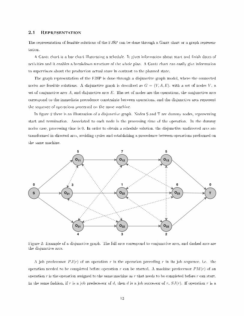
In �gure 2 there is an illustration of a disjunctive graph. Nodes S and T are dummy nodes, representing

start and termination. Associated to each node is the processing time of the operation. In the dummy

nodes case, processing time is 0. In order to obtain a schedule solution, the disjunctive undirected arcs are

transformed in directed arcs, avoiding cycles and establishing a precedence between operations preformed on

the same machine.

Figure 2: Example of a disjunctive graph. The full arcs correspond to conjunctive arcs, and dashed arcs arethe disjunctive arcs.

A job predecessor PJ(r) of an operation r is the operation preceding r in its job sequence, i.e. the

operation needed to be completed before operation r can be started. A machine predecessor PM(r) of an

operation r is the operation assigned to the same machine as r that needs to be completed before r can start.

In the same fashion, if r is a job predecessor of d, then d is a job successor of r, SJ(r). If operation r is a

13

machine predecessor of d, then d is a machine successor of r, SM(r).

Having established the sequence of operations, deciding which disjunctive arcs will become conjunctive

arcs, the makespan can be calculated. Since each node represents an activity with a duration time associated,

an earliest starting time (sE) and a latest starting time (sL) can be calculated. The earliest starting time of

an operation is the earliest time an operation can begin respecting its precedence. The latest starting time

corresponds to the latest an operation can begin without delaying the completion time of the last job (i.e.

the makespan).

To determine the earliest starting time of each node in the solution graph, we begin by setting the

starting node S earliest starting time at zeros, sE(S) = 0. Then, the remaining earliest starting time are the

maximum of the earliest completion time of the job predecessor and its machine predecessor, equation (1).

Consequently, we can de�ne the earliest completion time (cE) as the earliest an operation can �nish being

processed, equation (2).

sE(r) = max{cE [PJ(r)], cE [PM(r)]} (1)

cE(r) = sE(r) + PTr (2)

To compute the latest starting time, we start from the termination node, T , and work backwards. After

determining the earliest starting time of termination node T , corresponding to the makespan, we set the

latest starting time of that node equal to the makespan as well, i.e. sL(t) = CM . Since the termination

node has an associated processing time of zero, the latest and earliest starting times are the same as the

correspondent completion times. The value of the latest completion time of an operation r is determined by

the minimum of the latest starting times of its job and of its machine successor, equation (3).

cL(r) = min{sL[SJ(r)], sL[SM(r)]} (3)

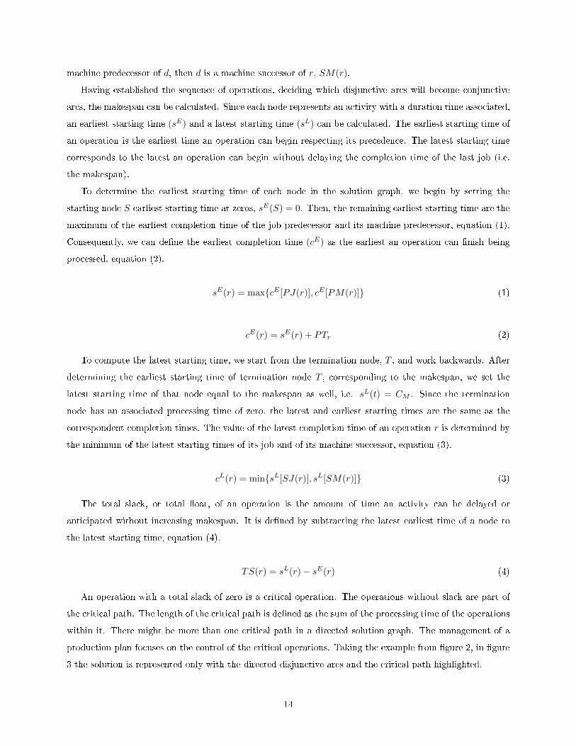
The total slack, or total �oat, of an operation is the amount of time an activity can be delayed or

anticipated without increasing makespan. It is de�ned by subtracting the latest earliest time of a node to

the latest starting time, equation (4).

TS(r) = sL(r)− sE(r) (4)

An operation with a total slack of zero is a critical operation. The operations without slack are part of

the critical path. The length of the critical path is de�ned as the sum of the processing time of the operations

within it. There might be more than one critical path in a directed solution graph. The management of a

production plan focuses on the control of the critical operations. Taking the example from �gure 2, in �gure

3 the solution is represented only with the directed disjunctive arcs and the critical path highlighted.

14

Figure 3: Example of a disjunctive graph with a determined sequence. Arcs in bold correspond to the criticalpath

2.2 Performance Measures and Objectives

Di�erent types of objectives and performance measures represent a great deal of importance in manufacturing

plants. Performance measures enable the quanti�cation of relevant aspects while the objectives mainly

determine how the schedule must be created. A review of the most important objectives is presented below.

Throughput and Makespan

Depending on the industry, company, and market strategy among other factors, maximizing the throughput

represents the most important performance indicator.

Throughput is computed by the output rate and is often limited by the bottleneck machines, which tend

to be plant's lowest capacity machines. In this situation, it is important to guarantee that the bottleneck

machine is never idle, which may require to have operations on the machine queue. On the other hand, if one

�nds sequence dependent setup times, then there must be an e�ort to minimize the sum of the setup times

on the bottleneck machine.

Makespan plays an important when dealing with a �nite number of jobs. The makespan is represented

as Cmax and is de�ned as the time when the last job leaves the system.

Cmax = max(C1, ..., Cn) (5)

where Cj is the completion time of job j. The objective of minimizing makespan and maximizing is closely

related.

15

Due Date

An important due date related measure is the lateness. Typically, one tries to minimize the maximum

lateness. A job lateness, Lj , is de�ned as

Lj = Cj −Duej (6)

where Duej denotes the job due date. The maximum lateness is then

Lmax = max(L1, ..., Ln) (7)

The objective of minimizing the maximum lateness is a consequence of trying to minimize the job lateness

that represents the worst performance on schedule.

The number of tardy jobs may also be taken as an objective, qualifying whether or not the job is tardy,

instead of measuring how late it is. It is more often to �nd tardy jobs considered as measure instead of an

objective, since if one envisions to minimize the number of tardy jobs, it is possible to end with a schedule

with very tardy jobs, which may be intolerable in practice.

To handle this the concept of total or average tardiness may be de�ned. The tardiness, Tj can be computed

as

Tj = max(Cj −Duej , 0) (8)

with the objective function as

n∑j=1

Tj (9)

It is interesting that none of the due date measures take into account and penalize the early completion

of a job. Since, the earlier the job is complete more storage and additional handling costs one can incur.

16

3 Static Scheduling

Scheduling is concerned with optimality of the allocation of limited resources over a time interval. Hence, a

manufacturing scheduling problem is about jobs, composed by operations that can be assigned to machines.

The assignment to machines constitutes the di�erence between the Job Shop Problem (JSP) and the Flexible

Job Shop Problem (FJSP). This apparently slight di�erence may largely increase the complexity of the

scheduling.

A static schedule over a time period requires information of the number of machines, number of jobs,

arrival times and due dates, in which machines the jobs operations may be executed, processing times for

each machine etc.. Most of the information required to create a schedule is known a priori. Although, the

shop �oor is dynamic a static scheduling is required for planning purposes. Planning in advance and reaching

the best possible solution may represent relevant cost savings for the plant.

In this chapter a deterministic and a meta-heuristic solution are presented. The former aims to exploit the

simple problem formulation and transform it in a Mixed Integer Linear Programming (MILP) problem. The

latter, is a Genetic Algorithm (GA) motivated by the NP-hardness and combinatorial nature of the problem

and provides a method that although not guaranteeing global optimal solutions does ensure solutions in

useful time. The GA here presented uses a hierarchical approach, along with a coding that guarantees

feasible solutions. Di�erent strategies were explored and combined to create the initial population, crossovers

and mutations. The solution quality is increased through local search, using a variable neighbourhood search.

Although MILP has been shown to be very limited in terms of problem size, it guarantees an optimal

solution. Hence, when small problem are concerned, it is still a very valuable resource. Moreover, it can be

used to guarantee a fairly good implementation of other algorithms, such as the proposed genetic algorithm.

3.1 Mixed Integer Linear Programming

With the increase in computational power in the beginning of the XXI century, Mixed Integer Linear Program-

ming (MILP), due to its rigorousness and modelling capabilities, was widely explored for NP-hard problems

[63]. In [63] two MILP formulations for equipment assignment and task allocation over time are presented.

First, considering discrete time, where the time horizon is discretized in uniform duration and decisions are

made in each sample of time. Second, in a continuous time formulation, where variable time intervals are

used marking events. This means that instead of discretizing the time horizon and only evaluating at �x step

sizes, evaluations take place when events occur.

Initially MILP for the FSJP modelled in a discrete time formulation [19, 20], which faces two main

limitations: (i) it is an approximation when compared to continuous time implementations, (ii) results in

an unnecessary increase of the binary variables, consequently increasing the size of the overall mathematical

problem, causing a severe impact on the computational time required. Thus more recently continuous time

Mixed Integer Linear Programming (MILP) have been used with several successful implementations for small

17

sized problems [16, 63, 22, 64].

With the aforementioned limitations of the discrete time MILP in mind, a continuous time formulation

based in [64] was implemented. Given the known di�culty of a mathematical model based solution to solve a

NP-hard and combinatorial problem as the FJSP, in order to reduce the mathematical optimization problem,

modi�cations that simplify and eliminate redundant variables were applied.

The model details are presented below.

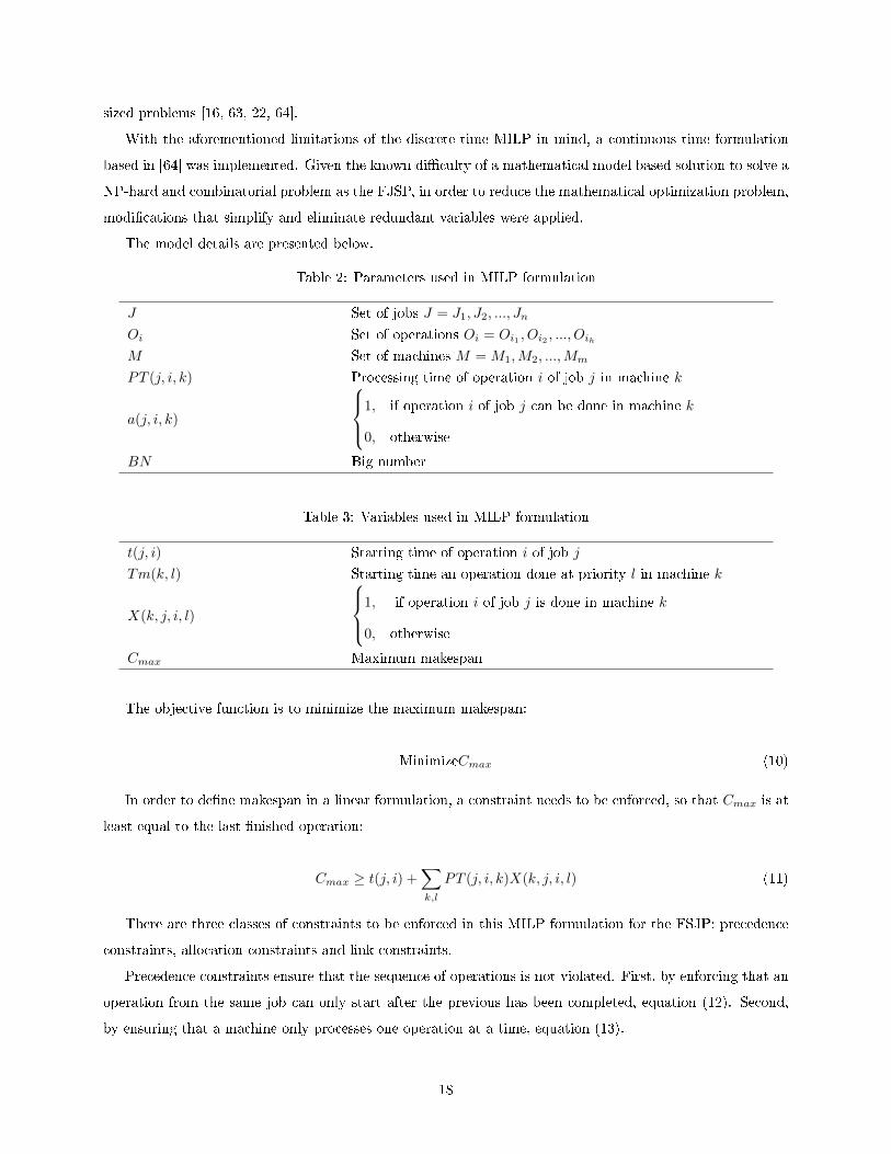
Table 2: Parameters used in MILP formulation

J Set of jobs J = J1, J2, ..., Jn

Oi Set of operations Oi = Oi1 , Oi2 , ..., OihM Set of machines M =M1,M2, ...,Mm

PT (j, i, k) Processing time of operation i of job j in machine k

a(j, i, k)

1, if operation i of job j can be done in machine k

0, otherwise

BN Big number

Table 3: Variables used in MILP formulation

t(j, i) Starting time of operation i of job j

Tm(k, l) Starting time an operation done at priority l in machine k

X(k, j, i, l)

1, if operation i of job j is done in machine k

0, otherwise

Cmax Maximum makespan

The objective function is to minimize the maximum makespan:

MinimizeCmax (10)

In order to de�ne makespan in a linear formulation, a constraint needs to be enforced, so that Cmax is at

least equal to the last �nished operation:

Cmax ≥ t(j, i) +∑k,l

PT (j, i, k)X(k, j, i, l) (11)

There are three classes of constraints to be enforced in this MILP formulation for the FSJP: precedence

constraints, allocation constraints and link constraints.

Precedence constraints ensure that the sequence of operations is not violated. First, by enforcing that an

operation from the same job can only start after the previous has been completed, equation (12). Second,

by ensuring that a machine only processes one operation at a time, equation (13).

18

t(j, i) +∑k,l

PT (j, i, k)X(k, j, i, l) ≤ t(j, i+ 1) (12)

Tm(k, l) +∑j,i

PT (j, i, k)X(k, j, i, l) ≤ Tm(k, l + 1) (13)

Allocation constraints need to be enforced to guarantee that a given operation is only allocated to one

machine, equation (15); that at the same time only one operation is being allocated to a given machine,

equation (14); and that operations are only being given to machines that can perform them, equation (16).

∑j,i

X(k, j, i, l) ≤ 1 (14)

∑k,l

X(k, j, i, l) = 1 (15)

∑l

X(k, j, i, l) ≤ a(j, i, k) (16)

Finally, it is important to force the starting time of an operation to be the same as the starting time of

the machine that will preform it, equations (17) and (18).

Tm(k, l) ≤ t(j, i) + (1−X(k, j, i, l))×BN (17)

Tm(k, l) + (1−X(k, j, i, l))×BN ≥ t(j, i) (18)

3.2 Genetic Algorithm

The genetic algorithm is a well known meta-heuristic based on an evolutionary algorithm. A meta-heuristic

is a high level heuristic able to search a very wide space of solutions and guide heuristics to escape local

minima. Although the genetic algorithm can �nd the optimal solution, it does not guarantee �nding the

global optimum. Because of the ability to search vast solution spaces, meta-heuristics are highly used and

recommended for large and complex problems.

The idea behind the genetic algorithm is the evolution of species. A genetic algorithm starts from an initial

population of solutions. Then, the whole population is scored against the objective function, called �tness

function. The individuals, based on their scoring, will be selected to either (1) stay elites, maintaining their

chromosomes the same, (2) be parents for crossover, implying a mix of both parents to create an o�spring, or

(3) mutate, thus creating new generations. The best solution in each generation is saved. The optimization

stops when the stopping criterion is met, for instance, when the maximum number of generations is reached

19

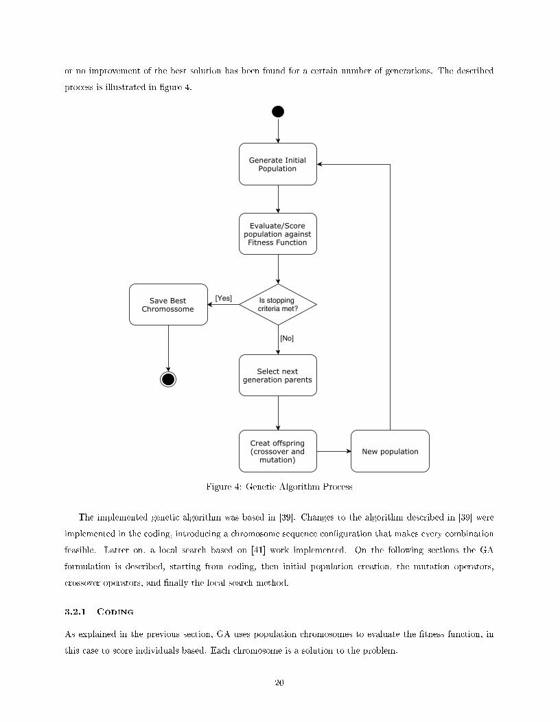
or no improvement of the best solution has been found for a certain number of generations. The described

process is illustrated in �gure 4.

Figure 4: Genetic Algorithm Process

The implemented genetic algorithm was based in [39]. Changes to the algorithm described in [39] were

implemented in the coding, introducing a chromosome sequence con�guration that makes every combination

feasible. Latter on, a local search based on [41] work implemented. On the following sections the GA

formulation is described, starting from coding, then initial population creation, the mutation operators,

crossover operators, and �nally the local search method.

3.2.1 Coding

As explained in the previous section, GA uses population chromosomes to evaluate the �tness function, in

this case to score individuals based. Each chromosome is a solution to the problem.

20

Chromosomes are strings of information. In [39] chromosome entries correspond to strings (j, k,m), one

by operation, where j is the job, k is the operation and m the machine that is going to perform it. The

order in which these strings appear in the chromosome is the sequence. This representation is called task

sequencing list. The drawback of these representations is that attention should to be paid when generating

the o�spring to make sure the solution is feasible, i.e. the operation order constraint is not violated.

So that the sequence feasibility would not be an issue, a di�erent coding system was used, based in [65].

The used coding representation is often refered as operation − based representation, where the �rst half of

the chromosome corresponds to the assignment of jobs to machines and the second to the sequencing.

The assignment part of the chromosome is done in a vector form, where the vector entry (i, k) corresponds

to the machine m preforming operation k of job i. In table 4 is an example of the assignment part of the

chromosome, where operation O11 is assigned to machine 3 and operation O12 to machine 2.

Table 4: Assignment part of the chromosome

O11 O12 O13 O21 O22 O31 O32

3 2 2 2 3 1 3

The chromosome sequencing part is the second half of the chromosome and is based on the idea that the

�rst operation will start as soon as possible, i.e. if all machines are available at time t = 0, then the �rst

operation will start at that time. With this assumption, the time variable is taken out of the optimization,

sequence becoming the only concern. The sequencing section has the same length as the assignment one.

The entries are the job to be sequenced there, meaning that the �rst time entry 1 appears, it corresponds

to operation O11, and the second time to O12. By doing this all sequence combinations will be feasible. An

example of the sequencing chromosome section can be seen in table 5.

Table 5: Sequencing part of the chromosome

1 2 3 1 2 3 1

The resulting chromosome is the combination of table 4 and table 5. The Gantt chart resulting from the

decoding is in �gure 5, where the Makespan is 13 time units.

21

Figure 5: Gantt chart result of example chromosome assignment and sequence represented in table 4 and 5,respectively

3.2.2 Initial Population

The initial population is created in two stages. First, the assignment part of the chromosome is created; and

then the sequencing part.

For the �rst stage, one of two methods are used, all based on a combination of both processing time and

machine workload. The �rst method - smallest processing time method - follows the process described below,

and the �rst steps as well as the �nal assignment result are illustrated in table 6:

1. Find in the processing time table the smallest processing time and �x that assignment;

2. Add to the rest of the operations in that column the processing time corresponding to the operation

�xed;

3. Return to point 1 excluding the already �xed rows, until all operations are assigned.

22

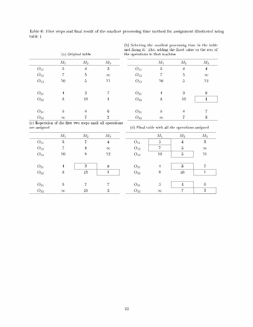
Table 6: First steps and �nal result of the smallest processing time method for assignment illustrated usingtable 1

(a) Original table

M1 M2 M3

O11 5 4 3

O12 7 5 ∞O13 10 5 11

O21 4 3 7

O22 8 10 1

O31 5 4 6

O32 ∞ 7 2

(b) Selecting the smallest processing time in the tableand �xing it. The, adding the �xed value to the rest ofthe operations in that machine

M1 M2 M3

O11 5 4 4

O12 7 5 ∞O13 10 5 12

O21 4 3 8

O22 8 10 1

O31 5 4 7

O32 ∞ 7 3

(c) Repetition of the �rst two steps until all operationsare assigned

M1 M2 M3

O11 5 7 4

O12 7 8 ∞O13 10 8 12

O21 4 3 8

O22 8 13 1

O31 5 7 7

O32 ∞ 10 3

(d) Final table with all the operations assigned

M1 M2 M3

O11 5 4 3

O12 7 5 ∞O13 10 5 11

O21 4 3 7

O22 8 10 1

O31 5 4 6

O32 ∞ 7 2

23

The second method for assignment, the reordering method, is similar to the �rst, but this time a shu�ing

of the table rows is done �rst, maintaining the operation order, and then a search for the minimum goes row

by row starting at the beginning of the table. The steps are as follows:

1. Shu�ing of job order in the processing time table;

2. By row �nd the minimum of processing time and �x that assignment;

3. Add to the rest of the operations in that column the processing time corresponding to the operation

�xed.

The �rst steps and the �nal result of this method applied to table 1, are shown in table 7. While the

previous assigning method has a small amount of di�erent outcomes, this second assignment method is highly

dependant on the randomly chosen job order.

After the assignment is done, the sequencing can be done with one of the following three rules:

1. Randomly select a job;

2. Job with most work yet to be done (sum of processing time in the assigned machines) - MWR;

3. Job with most highest of operations yet to be done - NOR;

24

Table 7: First steps and �nal result of the reordering assignment method illustrated using table 1

(a) Original table

M1 M2 M3

O11 5 4 3

O12 7 5 ∞O13 10 5 11

O21 4 3 7

O22 8 10 1

O31 5 4 6

O32 ∞ 7 2

(b) Shu�ing of job order in the processing time table

M1 M2 M3

O31 5 4 6

O32 ∞ 7 2

O21 4 3 7

O22 8 10 1

O11 5 4 3

O12 7 5 ∞O13 10 5 11

(c) Selecting the smallest processing time in the �rst rowand �xing it. Then, adding the �xed value to the rest ofthe operations in that machine

M1 M2 M3

O31 5 4 6

O32 ∞ 11 2

O21 4 7 7

O22 8 14

O11 5 8 3

O12 7 9 ∞O13 10 9 11

(d) Repetition of the the previous step for the followingrow

M1 M2 M3

O31 5 4 8

O32 ∞ 11 2

O21 4 7 9

O22 8 14 3

O11 5 8 5

O12 7 9 ∞O13 10 9 13

(e) Randomly ordered table with all the operations as-signed

M1 M2 M3

O31 5 4 6

O32 ∞ 7 2

O21 4 3 7

O22 8 10 1

O11 5 4 3

O12 7 5 ∞O13 10 5 11

(f) Final table with all the operations assigned

M1 M2 M3

O11 5 4 3

O12 7 5 ∞O13 10 5 11

O21 4 3 7

O22 8 10 1

O31 5 4 6

O32 ∞ 7 2

25

3.2.3 Mutation Operators

After the selection of parents for mutation is completed, one of three di�erent mutation operators can be

applied:

1. Precedence Preserving Shift mutation (PPS) [66, 39];

2. Assignment mutation;

3. Intelligent mutation [39].

PPS mutation alters the sequence part of the chromosome. This operator randomly selects one operation

and moves it to another position in chromosome. An example of PPS mutation is shown in �gure 6. It is

important to mention that, because of the way the coding is done, there are no concerns about the feasibility

of the new solution.

Assignment mutation chooses a single operation assignment randomly and changes the assignment to

another randomly chosen machine. If the operation chosen cannot be preformed on any other machine, the

process is restarted until either an operation can be done on another machine or there are no more operations

to investigate.

Finally, intelligent mutation consists on selecting an operation from the machine with maximum workload

and assigning it to the one with minimum workload. If it is not compatible no mutation occurs.

Figure 6: Illustration of Precedence Preserving Shift mutation. The �rst operation of job 3 will take thesequence's 5th position.

3.2.4 Crossover Operators

The crossover operators use two parents to generate an o�spring. In this work, two types of crossover operator

were used. One to preform crossover in the assignment section of the chromosome, assignment crossover, and

another in the sequential section, Precedence Preserving Order-based crossover (POX) [66].

The assignment crossover mixes the assignment from both parents. At �rst, a set of randomly selected

operations are copied from parent one to the o�spring. The remaining operations assignment is copied from

the second parent. The sequencing is maintained from the �rst parent to the o�spring.

26

POX operator selects from the �rst parent a job to copy the sequence. The selected job sequence is copied

to the o�spring, and the rest of the jobs are taken from the second parent in the order in which they appear.

In this operator the assignment is maintained from the �rst parent to the o�spring.

(a) Assignment crossover operator. Only the assignmentsection of the chromosome is illustrated.

(b) POX crossover operator. Only the sequence section ofthe chromosome is illustrated.

Figure 7: Crossover Operators.

3.2.5 Variable Neighbourhood Search

The evolution convergence speed of standard GAs is extensively reported to be slow. A promising solution

for its improvement is the use of local search algorithms along with GA. A hybridized GA with local search

envisions the introduction of a local optimizer that is applied to every children before its insertion into the

population. Hence, the space of solutions global exploration is in charge of GA, while the local search explores

the chromosome features and may introduce problem speci�c knowledge in the form of rules or conditions to

increase the solution quality and speed of convergence. To employ local search, a Variable Neighbourhood

Search (VNS) was introduced. VNS aims at exploring the neighbourhood space of solutions by trying to move

an operation, randomly chosen, from the bottleneck path to a feasible slot in a neighbour. An important

27

characteristic of VNS is that the solution quality never gets degraded, by only moving from one solution to

another if the recently obtained is better.

The VNS is applied after the crossover and mutation operators �rst by moving one operation and then

by moving two operations simultaneously. Both these operation moves are detailed in the remaining of this

section.

Moving one operations

A solution graph makespan is de�ned by the length of the critical paths, which is equivalent to say that

the makespan cannot be reduced if the critical paths are the same. The local search goal is to successively

identify and break the current critical paths to obtain a new schedule with smaller makespan.

The concept of critical operation, in simple words, is that if one removes an operation r and reallocates

in another feasible position, and the original critical path machine latest completion time does not increase,

then r is not a critical operation.

By taking the graph representation presented in section 2, if an operation r from the critical path, i.e.

an operation with a total slack of zero, is taken from a machine and inserted behind an operation with a

total slack of at least the same as the processing time of r, this second solution has at the most the same

makespan as the original. When moving an operation it is important to consider a few rules, taking r as the

moved operation and v as the candidate operation for r to be assigned before:

1. The total slack of v needs to be at least equal to the processing time of r in the candidate machine,

equation (19);

2. The latest possible starting time of operation v needs to be at least equal to the maximum between the

earliest completion time of the job predecessor of v and r plus the processing time of r in the candidate

machine, equation (20);

3. The latest starting time of the job successor of r needs to be at least equal to the maximum between the

earliest completion time of the job predecessor of v and r plus the processing time of r in the candidate

machine, equation (21).

TS(v) ≥ PT (r) (19)

sL(v) ≥ max{cE(r − 1), cE(v − 1)}+ PT (r) (20)

sL(r + 1) ≥ max{cE(r − 1), cE(v − 1)}+ PT (r) (21)

The pseudo-algorithm for this operation is in algorithm 1.

28

Moving two operations

Moving two operations was proven to be always better than moving one [29]. It consists of trying to move

two consecutive operations, and if one does not �nd an appropriate position, then a new combination of

operations is chosen. The pseudo-algorithm for this operation is in algorithm 2.

Algorithm 1 Moving an operation pseudo-algorithm

1: Identify critical path P

2: Set r as the �rst operation r from P

3: while Operation r is not assigned or r is not the last operation of P do

4: Delete r from graph

5: Search for an assignable interval for r

6: If an assignable interval is not found, set r to be the next operation in P

7: end while

8: if an interval was found then

9: Assign r to that interval

10: else

11: The current solution is a local minimum of moving one operation

12: end if

Algorithm 2 Moving two operations pseudo-algorithm

1: Identify critical path P

2: Set r as the �rst operation from P

3: while Operation r and v are not both assigned or r is not the last operation of P do

4: Delete r from graph

5: Identify the new critical path S

6: Set v as the �rst operation from S

7: while Operation r and v are not both assigned or v is not the last operation of S do

8: Delete v from graph

9: Search for an assignable interval for r

10: if an interval for r was found then

11: Assign r to that interval and search for an interval for v

12: end if

13: If neither an interval for r or v was not found, set v to be the next operation in S

14: end while

15: If an assignable interval is not found, set r to be the next operation in P

16: end while

29

4 Dynamic Scheduling

While static scheduling techniques can guarantee very good results, in real life plants events are dynamic,

generating gaps between predicted schedule outcome and the actual shop state.

Dynamic scheduling techniques are not upset by disturbances once the schedule can be done quickly at

almost real time. Typical dynamic scheduling methods are dispatching rules, simple heuristics and multi-

agent based systems. Multi-agent based systems are systems composed of autonomous agents representing

each of the factories physical entities. The motivation to employ agent based systems in dynamic scheduling

is manifold. First, they have the advantage of behaving in a distributed way, each agent being responsible

for local scheduling of one or two entities, yielding a highly �exible system. Second, the distributed system

enables very fast scheduling, once the schedule is not globally generated, but emerges from the combination of

many di�erent local schedules. And last, each entity software is simpler than a global approach and, by being

independent, enables to easily remove or add entities without any changes in the network software. Multi-

agent based solutions are appointed as a very promising area of research in dynamic scheduling, although

there is still some lack of research in this topic [13]. The drawback of many of these methods, however, is

the lack of horizon driven from the local decision making, generating schedule solutions far from optimal.

For the dynamic scheduling part of this thesis, a multi-agent based system method will be presented,

using ant based communication between agents. To combat the stated myopia associated with this type of

systems, a prediction horizon was added and the agent based architecture changed from an autonomous to

a mediator architecture. Both methods, the autonomous and the mediator architecture are described in the

throughout this chapter.

4.1 Autonomous Ant Based System

A multi-agent based system inspired in ant behaviour was implemented based on [52] approach. In a this

agent architecture, multiple agents are responsible for di�erent parts of the system. The whole system success

is highly dependent on their ability to communicate and coordinate tasks. In the proposed method, four

functional agents are used, table 8. All agents are in the same hierarchy level and there is no agent evaluating

the global plant performance. This type of organization is described as an autonomous architecture.

When orders arrive they are assigned to order agents, which then register to the shop agent. Order

agents only have two states, in process, since they are registered, and complete, when the order is �nished.

The shop agent is responsible for updating agent status. Once the order is registered, jobs, which can have

multiple operations, are assigned to job agents. Job agents requests shop agent for resources, then shop

agent searches for the resources and provides feedback. Interaction between job agents and machine agents

starts. First, machine agents make a proposal to job agents based on their status, queue and processing time

of that combination of operation and machine. Job agents evaluate machine proposal and determine which

machine they should follow to. When the machine is determined, each job agent makes a proposal to machine

30

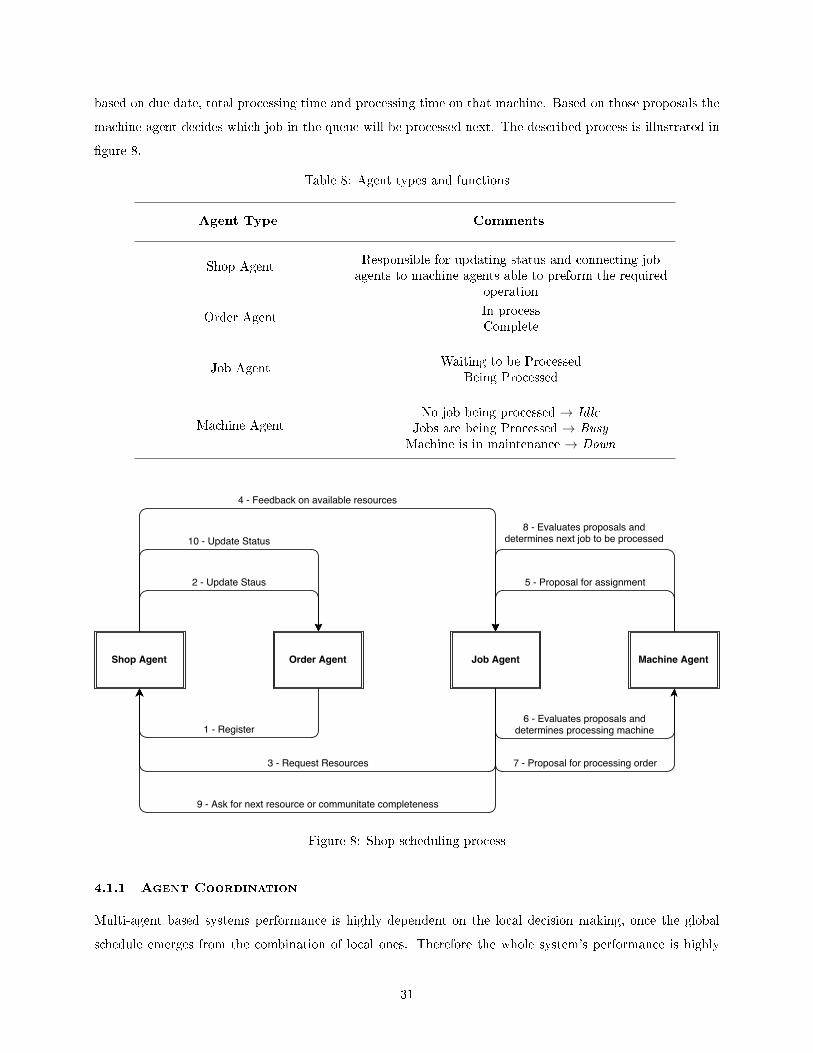
based on due date, total processing time and processing time on that machine. Based on those proposals the

machine agent decides which job in the queue will be processed next. The described process is illustrated in

�gure 8.

Table 8: Agent types and functions

Agent Type Comments

Shop AgentResponsible for updating status and connecting jobagents to machine agents able to preform the required

operation

Order AgentIn processComplete

Job AgentWaiting to be Processed

Being Processed

Machine AgentNo job being processed → Idle

Jobs are being Processed → BusyMachine is in maintenance → Down

Figure 8: Shop scheduling process

4.1.1 Agent Coordination

Multi-agent based systems performance is highly dependent on the local decision making, once the global

schedule emerges from the combination of local ones. Therefore the whole system's performance is highly

31

dependent on the coordination between agents. Many coordination protocols have been developed with

various di�erent advantages and drawbacks. These protocols can be classi�ed as market negotiation, auction

negotiation or insect inspired communication. In this work multi-agent based system uses an insect inspired

coordination based on ant colony behaviour.

[61] developed a meta-heuristic optimization called Ant Colony Optimization, ACO, that is based on the

self-organization behaviour of ant colonies. The ant inspired optimization is driven by the ability of ants to

�nd the shortest path between food and nest, even when an obstacle appears in their way. When walking

they deposit pheromones, which are used as communication method, once each ant chooses, preferably, the

path with higher pheromone intensity.

The behaviour described above explains how ants follow the shortest connecting path between food and

nest. When an obstacle blocks their path, about half of the ants follow around one side of the obstacle and

the rest around the other side, �gure 9b. When they �nd food, they go back to the nest through the same

path they had followed before, depositing pheromones once again. Pheromones fade away at a certain rate

of decay, and therefore a higher pheromone intensity will be found in the shortest path, �gure 9c. Since ants

tend to prefer paths containing a higher pheromone intensity, the ant colony will always follow the shortest

path until another obstacle appears, �gure 9d.

(a) Ants go from the nest to the food and back (b) An obstacle comes in their way. Ants choose one sideto go around it with equal probability

(c) There is a higher pheromone intensity in the shortestpath

(d) Ants tend to go through the path containing higherpheromone intensity, which corresponds to the shortest

Figure 9: Organizational methodology of an ant colony searching for food.

The arti�cial ants used in this algorithm have many di�erences from both the real ants described above,

and the arti�cial presented in [61]:

1. Di�erences from real ants

• When making a decision, not only the pheromones are considered but also a heuristic function

• Ants have memory, in the sense that they know which operation has already been done

32

2. Di�erences from both real ants and arti�cial ants described in [61]

• Pheromones do not fade, they are just updated based on agent status

• Heuristic function is function of processing time, which can be seen as a path length

• Pheromones are functions of processing time, or both processing time and due date. Meaning that

the more urgent the deadline gets, the highest the pheromone associated with that agent.

Both job agents and machine agents make decisions, so both have associated pheromones, τMach and

τJob. Machine pheromones are related to how fast a job processing can be started on that machine, taking

in consideration the rest of the jobs in line. This means that the longer the machine queue, the lower the

pheromone intensity associated to the machine. However, the job associated pheromones are related to how

much time it has left before due date, subtracting the work yet to be done. This means that even if a job

has a due date very close, another job with more time until due date will have a higher pheromone value if

it has more work left to be done.

The multi-agent based method presented works in two stages. First, it starts by assigning jobs to opera-

tions. Second, it sequences jobs on each machine.

A job is assigned to the machine with the highest bidding. The bidding of a machine for a job is given by

equation (24). In this bidding, pheromone function τMach and heuristic function η are weighted by parameter

α and β, respectively. The machine pheromone intensity is given by equation (22). A machine has three

di�erent status:

1. Idle: There is no job assigned to that machine. Then the pheromone will be 1

2. Busy : The pheromone value is as low as the sum of processing times of the jobs in queue, assigned to

that machine. It is given by equation (22), where xMachiis 1, because the machine is available, and qikl

is 1 if operation l of job k is in queue in machine i, and 0 otherwise. PT ikl corresponds to the processing

time of operation l of job k in machine i.

3. Down: If a machine is in maintenance, its pheromone value is 0. Taking equation (22), it corresponds

to setting parameter xMachito 0.

The heuristic function associated to each machine i is given by the inverse of the processing time of

operation l of job k in machine i, (23). Given this and looking at equation (24), if only the heuristic is used

to compute the machine bidding function, equivalent to setting α = 0, the machine assignment would be

done in a shortest processing time fashion.

Parameters α and β are tunable for changing the relative weight of pheromones and heuristic when making

an assignment decision.

τMachi(t) =xMachi∑

k

∑l qiklPT

ikl

(22)

33

ηikl =1

PT ikl(23)

p(MAi) =(τMachi)

α(ηikl)

β∑j (τMachj )

α(ηjkl)

β(24)

The second stage of the algorithm, the sequencing phase is through a competition of biddings between

the jobs assigned to the same machine. Meaning that if there is more than one job assigned to the same

machine, the machine agent needs to decide which job will be processed next. Hence, job agents will bid for

their turn in the machine. The bidding function, equation (26), works as well with a weighted combination

of pheromones and heuristic function.

The heuristic function is the same as the one used for the machine bidding, (23). It is calculated through

the inverse of the processing time of the job's operation in the associated machine.

The pheromone function is given by equation (25), where term fl is associated to operation l of job k and

takes value 1 if that operation is not completed or 0 if otherwise. The pheromone value is a function of how

close their due date is and how much time they still need to be completed. Once the pheromone function

behaves as the known function f(x) = exp(−x), as time goes by and the job is approaching its deadline, if

there is still a lot left to be down, the pheromone value will increase exponentially.

τJobk(t) = exp−

(DueJobk −

(t+

∑l

flPTkl

))(25)

p(Jobi) =(τJobi)

α(ηiil)

β∑k (τJobk)

α(ηkkl)

β(26)

To understand how the above equations connect to allocate jobs, a description of the implementation can

be analysed in algorithm 3.

34

Algorithm 3 Multi-ant-like agents pseudo-algorithm

1: for time = 1 : timemax do

2: Generate jobs

3: if job is generated then

4: n← n+ 1

5: end if

6: for k = 1 : n do

7: op(k)← next operation of job i

8: WorkCenter(k)← group of machines where op(k) can be preformed

9: for i = 1 : m do . For each machine

10: Compute heuristic function for each machine to preform operation op(k) of job k, ηikl

11: Compute pheromones of machine i at time t, τMachi(t)

12: Compute Probability of job k being processed in machine i, p(MAi)

13: end for

14: Compute pheromones of job k at time t, τJobk(t)

15: For machine i with maximum p(MAi), compute probability of job k being processed next, p(Jobk)

16: end for

17: The job with highest p(Jobk) will be processed next on the machine for which it has the highest

p(MAi)

18: end for

35

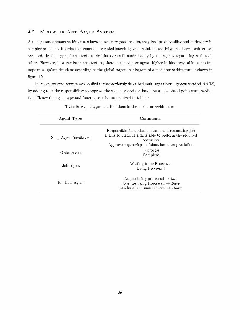
4.2 Mediator Ant Based System

Although autonomous architectures have shown very good results, they lack predictability and optimality in

complex problems. In order to accommodate global knowledge and maintain reactivity, mediator architectures

are used. In this type of architectures decisions are still made locally by the agents negotiating with each

other. However, in a mediator architecture, there is a mediator agent, higher in hierarchy, able to advice,

impose or update decisions according to the global target. A diagram of a mediator architecture is shown in

�gure 10.

The mediator architecture was applied to the previously described multi-agent based system method,AABS,

by adding to it the responsibility to approve the sequence decision based on a look-ahead point state predic-

tion. Hence the agent type and function can be summarized in table 9.

Table 9: Agent types and functions in the mediator architecture

Agent Type Comments

Shop Agent (mediator)

Responsible for updating status and connecting jobagents to machine agents able to preform the required

operationApprove sequencing decisions based on prediction

Order AgentIn processComplete

Job AgentWaiting to be Processed

Being Processed

Machine AgentNo job being processed → Idle

Jobs are being Processed → BusyMachine is in maintenance → Down

36

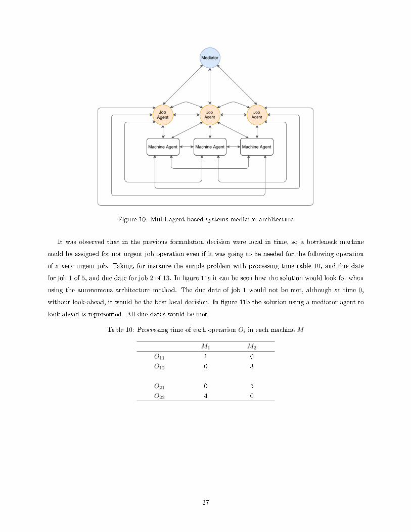
Figure 10: Multi-agent based systems mediator architecture

It was observed that in the previous formulation decision were local in time, so a bottleneck machine

could be assigned for not urgent job operation even if it was going to be needed for the following operation

of a very urgent job. Taking, for instance the simple problem with processing time table 10, and due date

for job 1 of 5, and due date for job 2 of 13. In �gure 11a it can be seen how the solution would look for when

using the autonomous architecture method. The due date of job 1 would not be met, although at time 0,

without look-ahead, it would be the best local decision. In �gure 11b the solution using a mediator agent to

look-ahead is represented. All due dates would be met.

Table 10: Processing time of each operation Oi in each machine M

M1 M2

O11 1 0

O12 0 3

O21 0 5

O22 4 0

37

(a) Result of the MABS with autonomous architecture for the problem stated in table 10. Since due datejob 1 would be 4 and of job 2 would be 13,in this �gure it can be seen that the job 1 would not meet thedeadline.

(b) Solution for the problem stated in table 10, respecting due dates.

Figure 11: Crossover Operators.

To mitigate e�ect of this myopia, changes to the previous method were done:

1. There are agents for both current job operation and agents for following job operation;

2. The process of machine assignment and sequencing is done on both types of job agents separately;

3. If there is both a current job agent and a following job agent bidding for the same machine and sequenced

as next, the mediator acts to solve the situation.

For the mediator to solve the situation, a pheromone contest between the next current job agent and the

following job agent is done. In a horizon corresponding to the current job agent processing time, pheromones

are calculated and compared for both agents. Then, if in all time intervals the current job agent had a

higher pheromone value, the current job agent is sequenced for that machine. On the other hand, if in any

of those time intervals the next job agent shows a higher pheromone intensity value, the machine waits for

the operation corresponding to the following job agent to be assigned by a current job agent.

38

5 Results and Discussion

In this section results from the afore mentioned methods are presented. First, the MILP is tested against some

job shop and �exible job shop problem datasets. Afterwards, the genetic algorithm is tuned to some extent

and compared with FSJP benchmarks. The need for the local search extension in this method is presented

and results are shown incorporating it. Finally, the two dynamic multi-ant-like architectures, AABS and

MABS are compared in a dynamic environment.

5.1 MILP

The MILP algorithm was tested against Hurink instances [67]. Hurink instances are divided into four sets:

• sdata: Job shop problems, i.e. operations are assignable to exactly one machine. Lower bounds for

these instances can be consulted in [29];

• edata: Some operations may be assigned to more than one machine;

• rdata: Most operations may be assigned to several machines;

• vdata: All operations may be assigned to several machines.

At �rst, MILP was tested in the least complex sdata instance, mt06s, a JSP consisting of 6 jobs with 6

operations each and 6 machines. Once it was able to solve it and reach it's lower bound, the MILP algorithm

was tested in second least complex sdata instance, mt10s, consisting of 10 jobs, 10 operations each and 10

machines. MILP was not able to solve mt10s instance. The Gantt chart for the mt06s instance is in �gure

12.

While MILP could not solve problems when the number of jobs was increased, it was able to solve problems

when shop �exibility was added. To test this, a new dataset was created. It consisted of the mt06e, the

simplest Hunrik instance from sdata, with only the �rst three jobs. This instance is named here as mt03e, it

has 3 jobs, with 6 operations each and 6 machines. The instance was solved by the MILP algorithm and the

Gantt chart of the solution is in �gure 13. Because MILP successfully solved mt03e it was tested in mt06e,

an instance similar to mt06s but with machine �exibility. It was again successful and the Gantt chart is in

�gure 14. Once again, when trying to increase the complexity to next instance mt10e the algorithm was not

able to �nd a solution.

The obtained results were also used to validate the genetic algorithm, GAJobS, implementation. As

presented in table 11, the genetic algorithm without Variable Neighbourhood Search was able to, as well as

the MILP algorithm, reach the best known lower bound.

It was because of the lack of ability of the deterministic algorithm, MILP, to �nd solutions for higher

complexity problem that it was decided to move to a meta-heuristic optimization method, the genetic al-

gorithm. However, it is important to state that the MILP results are highly limited by the software it was

39

implemented on. The software used was Matlab 17a. Matlab linear programming software is still being up-

dated and maybe, either in future Matlab versions, and probably in CPLEX IBM software, the algorithm

would be able to solve harder problems than the ones presented here.

Table 11: Makespan obtained and best known Lower Bound (LB) using the MILP algorithm and the GAJobs.

Instance No. JobsNo.

Machines

No. Operations

per JobLB MILP GAJobS

mt06s 6 6 6 55 55 55

mt03e 3 6 6 N.A. 47 47

mt06e 6 6 6 55 55 55

0 10 20 30 40 50

Time units

M1

M2

M3

M4

M5

M6

Machines

MILP mt06s with Cmax = 55

Job1

Job2

Job3

Job4

Job5

Job6

Figure 12: Gantt chart and makespan for mt06s instance using MILP algorithm (Cmax = 55)

40

0 10 20 30 40 50

Time units

M1

M2

M3

M4

M5

M6

Machines

MILP mt03e with Cmax = 47

Job1

Job2

Job3

Figure 13: Gantt chart and makespan for mt03e instance using MILP algorithm (Cmax = 47)

0 10 20 30 40 50

Time units

M1

M2

M3

M4

M5

M6

Machines

MILP mt06e with Cmax = 55Job1

Job2

Job3

Job4

Job5

Job6

Figure 14: Gantt chart and makespan for mt06e instance using MILP algorithm (Cmax = 55)

41

5.2 Genetic Algorithm

The results obtained for the static scheduling using the genetic algorithm are presented here. The developed

genetic algorithm was tested using Brandimarte 10 problem instances with medium �exibility [27]. The

parameters of the instances are in table 12, where |Mi,k| indicates de maximum number of assignable ma-

chines per operation. P.T ime corresponds to the limits employed on a uniform distribution to compute the

processing time. It is possible to drive from table 12 that the instances complexity increases both in number

of jobs as in number of machines.

Based in this �exible job shop problem, the genetic algorithm was tuned in terms of initial population,

population size and crossover fraction. The tuning process is described below.

Table 12: Brandimarte dataset instances characteristics. Lower and upper bounds correspond to makespan(Cmax).

InstanceNo.

Jobs

No.

Machines

No. Operations

per Job|Mi,k| P. Time LB UB

Mk01 10 6 5...7 3 1...7 36 39

Mk02 10 6 5...7 6 1...7 24 26

Mk03 15 8 10 5 1...20 204 204

Mk04 15 8 3...10 3 1...10 48 60

Mk05 15 4 3...10 2 5...10 168 172

Mk06 10 15 15 5 1...10 33 58

Mk07 20 5 5 5 1...20 133 139

Mk08 20 10 5...15 2 5...20 523 523

Mk09 20 10 10...15 5 5...20 299 307

Mk10 20 15 10...15 5 5...20 165 197

5.2.1 Initial Population Creation

The genetic algorithm is an evolutionary algorithm that starts from an initial population of solutions and

evolves by combining individuals. Hence, the initial solutions may determine the solution space explored. It

is important that these solutions, are not only good solutions but signi�cantly di�erent.

In the implemented genetic algorithm, the population creation is two-folded. First, the assignment section

of the chromosome is generated and second, based on the assignment, the sequence section is decided.

For the assignment phase there are two creation methods: the smallest processing time method and the

reordering method. The smallest processing time method yields very good solutions, but the solutions are

not very di�erent from each other, once the only time a di�erence may occur is in case there are concurrent

processing time minimums in the processing time table. On the other hand, the reordering assignment

method is very stochastic, which tends to increase the solution variability, but it does not guarantee good

solutions.

42

For the sequencing section there are three alternative formulation methods. The �rst method is to

randomly select jobs and sequence them on the �rst available space. The second is to assign jobs by order of

most work yet to be done. The third is to select jobs by order of the higher number of operations still needed

to be done. Similarly to before, in the sequencing methods, although the second and third methods have a

good chance of yielding good solutions, both will have a very low variability of solution. On the contrary, for

the �rst sequencing method very high variability is expected.

Keeping in mind the afore mentioned algorithm characteristics it was decided that the second sequencing

method (MWR) and third (NOR) would have the same probability of occurring. By doing this the tuning

of the initial population creation was reduced to two variables, x and y:

• Probability of an individual of initial population being assigned using smallest processing time method:

1− x

• Probability of an individual of initial population being assigned using reordering method: x

• Probability of an individual of initial population being sequenced using random job selection: y

• Probability of an individual of initial population being sequenced using MWR: 0.5× (1− y)

• Probability of an individual of initial population being sequenced using most operations remaining:

0.5× (1− y)

In �gure 15 shows the mean and standard deviation of the �tness of the initial population when varying

the assignment using reordering method fraction and the sequencing using random job selection fraction. It

was chosen that in order to have a good initial population, a high variance with a maintaining a low average

�tness value would be the goal. Hence, based on the results shown in �gure 15 the values chosen for the

initial population creation are 0.6 using reordering method assignment and 0.6 using random job selection

sequencing.

5.2.2 Population Size

The population size in an evolutionary algorithm plays a very relevant role in the simulation results. If

the chosen population is too small, the algorithm may converge too early and not provide an adequate

solution space exploration. On the other hand, if a population size is chosen too large it may take a lot of

computational e�ort to converge. Regarding this topic [68] suggests that a population size of around 10 times

the number of decision variables is usually a reasonable size for an evolutionary algorithm.

Regarding the importance of the population size in the results a convergence solution analysis was pre-

formed. From the problems presented in table 12, the one with more variables and possible combinations is

Mk10. Therefore that problem was chosen to decide the population size. The population size analysis was

performed with standard parameters for a population of 500 to 5000 individuals and results of 5 runs were

analysed. The results of the population size convergence are presented in �gure 16, showing both mean and

43

Mean Fitness of Initial Population

0 0.2 0.4 0.6 0.8 1

Reordering Assignment method fraction

0

0.2

0.4

0.6

0.8

1Random

jobselectionsequencingmethodfraction

62

64

66

68

70

72

74

76

78

(a) Mean makespan for the initial population created with di�erent combinations of fractions of assignment usingreordering method and random selection.

Fitness function Standard Deviation of Initial Population

0 0.2 0.4 0.6 0.8 1

Reordering Assignment method fraction

0

0.2

0.4

0.6

0.8

1Random

jobselectionsequencingmethodfraction

3

4

5

6

7

8

9

10

11

12

(b) Standard deviation of makespan value for the initial population created with di�erent combinations of fractionsof assignment using reordering method and random selection.

Figure 15: Initial population �tness value when varying the assignment and sequencing methods fractions.

standard deviation of makespan over the 5 runs. It can be seen that the solution converges for a population

size of about 4000 individuals maintaining the mean makespan. Although standard deviation increases in

the last three population sizes, contrary to the expected behaviour, it may only be due to the small amount

of runs.

In light of the previous analysis, a population size of 4500 individuals was chosen. This value is also

coherent with the analysis of [68] since the number of decision variables in this problem is 480.

44

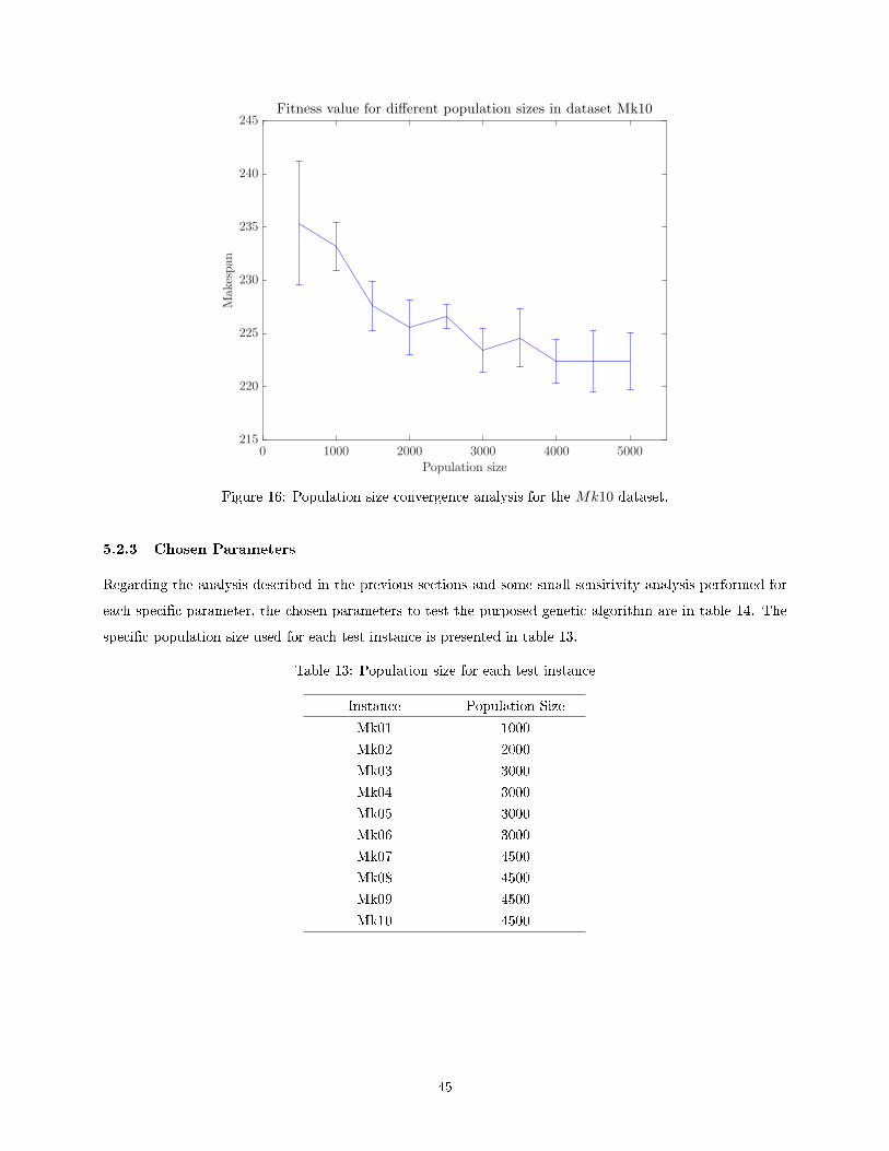
0 1000 2000 3000 4000 5000

Population size

215

220

225

230

235

240

245

Makespan

Fitness value for different population sizes in dataset Mk10

Figure 16: Population size convergence analysis for the Mk10 dataset.

5.2.3 Chosen Parameters

Regarding the analysis described in the previous sections and some small sensitivity analysis performed for

each speci�c parameter, the chosen parameters to test the purposed genetic algorithm are in table 14. The

speci�c population size used for each test instance is presented in table 13.

Table 13: Population size for each test instance

Instance Population Size

Mk01 1000

Mk02 2000

Mk03 3000

Mk04 3000

Mk05 3000

Mk06 3000

Mk07 4500

Mk08 4500

Mk09 4500

Mk10 4500

45

Table 14: Genetic algorithm parameters

Parameter Value

Initial Population

Assigned with smallest processing time method 0.4

Assigned with reordering method 0.6

Sequenced with random job selection 0.6

Sequenced with MWR selection 0.2

Sequenced with NOR method 0.2

Crossover Fraction 0.9

Crossover using assignment crossover 0.5

Crossover using POX crossover 0.5

Mutation Fraction 0.1

Mutation using PPS mutation 0.2

Mutation using assignment mutation 0.2

Mutation using intelligent mutation 0.6

Elite Fraction 0.01

Selection Method Roulette wheel

5.2.4 Results

The proposed genetic algorithm was tested with the Brandimarte problem described in table 12 using the

parameters stated in tables 14 and 13. All results were obtained after �ve runs, selecting the best individual.

Results were compared with four alternative genetic algorithms:

• Chen: In [36] proposed an innovative genetic algorithm for solving the �exible job shop problem. The

coding introduced in this paper split the chromosome in two sections, the �rst being routing policy and

the second the sequence of operations in each machine.

• GENACE: In [37] a GA with cultural evolution is introduced. In this algorithm, domain knowledge

is transmitted to the next generation. GA when applying crossover and mutation operators uses

information from previous generations of what kind of operations promoted good solutions.

• NGA: A recent approach proposed by [69]. The authors introduced a GA with a new chromosome

representation.

• hGA: In [41] the authors proposed a genetic algorithm with a variable neighbourhood descent search

after every iteration. Results show very good performance establishing new upper bounds.

• GAJobS: Approach proposed by the author.

46

The results are compared in table 15. Although the proposed algorithm was not within the best per-

forming, NGA and hGA, it produced good results when comparing to GENACE and Chen. Comparing

to GENACE it performed better in �ve of the nine datasets, and equally good in two of them. When

comparing to Chen it performed better in three out of ten and equally good in two out of ten.

To determine the reason for the di�erent results comparing to hGa a gantt chart for the Mk01 dataset

results was created, �gure 17. For a makespan of 40 time units to be obtained, regarding this is not a

completely �exible problem, the following changes needed to happen:

1. Job 9, Operation 6, that is currently in machine 2 would be reassigned to machine 4 where it has a

processing time of 6 time units;

2. Job 7, Operation 2, that is currently allocated to machine 4 would be reassigned to machine 1, where

it has a processing time of 3 time unit;

3. Job 6, Operation 4 and Job 8, Operation 4, would need to switch order in sequence of machine 2.

For GAJobS to arrive to this solution it would need either a great amount of running time, a very big

population or a lucky combination of permutations, crossovers and mutation. The unlikelihood combination

of these factors motivated the implementation of hGAJobS, the proposed genetic algorithm with a local

search optimization. The results for hGAJobS are presented in the next section.

Table 15: Makespan, Cmax, for the Brandimarte dataset (* represents best known Lower Bound).

Instance Chen[36] GENACE[37] NGA[69] hGA[41] GAJobS

Mk01 40 41 *37 40 42

Mk02 29 29 *26 *26 27

Mk03 *204 NA. *204 *204 *204

Mk04 63 67 *60 *60 67

Mk05 181 176 173 *172 176

Mk06 60 68 67 *58 65

Mk07 148 148 148 *139 143

Mk08 *523 *523 *523 *523 *523

Mk09 308 328 *307 *307 317

Mk10 212 231 212 *197 220

5.3 Hybrid Genetic Algorithm

The hybrid genetic algorithm, hGAJobS, is not as dependent on population size as the original GA presented.

This algorithm because of the local search converges faster with generally better solutions.

The parameters used were the same, excepting the population size. The population size for each tested

instance is presented in table 16. As can be observed, population size varies not according to the number of

variables within the problem but according to it's combinatorial complexity.

47

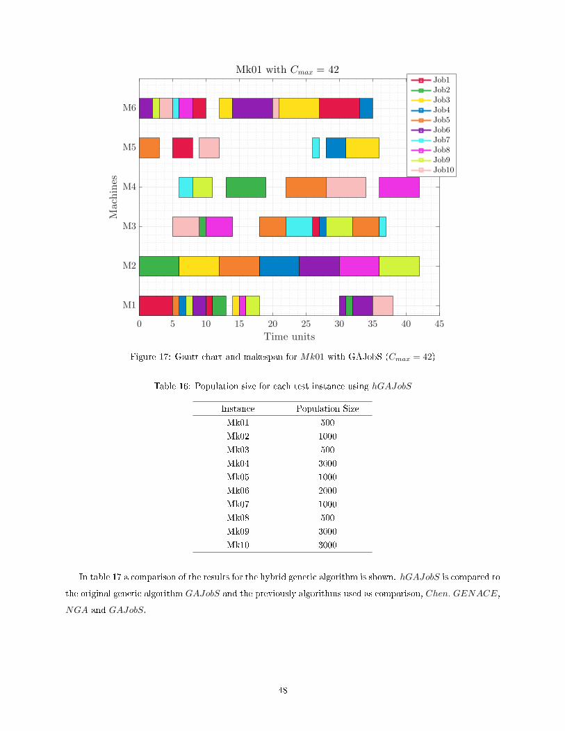
0 5 10 15 20 25 30 35 40 45

Time units

M1

M2

M3

M4

M5

M6Machines

Mk01 with Cmax = 42Job1

Job2

Job3

Job4

Job5

Job6

Job7

Job8

Job9

Job10

Figure 17: Gantt chart and makespan for Mk01 with GAJobS (Cmax = 42)

Table 16: Population size for each test instance using hGAJobS

Instance Population Size

Mk01 500

Mk02 1000

Mk03 500

Mk04 3000

Mk05 1000

Mk06 2000

Mk07 1000

Mk08 500

Mk09 3000

Mk10 3000

In table 17 a comparison of the results for the hybrid genetic algorithm is shown. hGAJobS is compared to

the original genetic algorithm GAJobS and the previously algorithms used as comparison, Chen, GENACE,

NGA and GAJobS.

48

Table 17: Makespan, Cmax, for the Brandimarte dataset (* represents best known Lower Bound).

Instance Chen[36] GENACE[37] NGA[69] hGA[41] GAJobS hGAJobS

Mk01 40 41 *37 40 42 40

Mk02 29 29 *26 *26 27 27

Mk03 *204 NA. *204 *204 *204 *204

Mk04 63 67 *60 *60 67 *60

Mk05 181 176 173 *172 176 173

Mk06 60 68 67 *58 65 64

Mk07 148 148 148 *139 143 141

Mk08 *523 *523 *523 *523 *523 *523

Mk09 308 328 *307 *307 317 312

Mk10 212 231 212 *197 220 211

Comparing to GAJobS, hGAJobS improved the solution in seven of the ten instances and maintain the

same makespan result in the other three, in which two of them were already optimal. We can see that

hGAJobS is a much more competitive algorithm than GAJobS. Although it did not preform as well as

hGA, it obtained very close results in seven of the ten instances. It is very likely that with more time and

maybe better tuned parameters, hGAJobS would reach the optimum solutions in more instances. hGAJobs

has clearly a similar performance as NGA, although NGA outperforms hGAJobs in instances Mk01, Mk02

and Mk09, hGAJobs presents better results for instances Mk06, Mk07 and Mk10. In comparison to Chen,

hGAJobs shows consistently better or similar results, excepting for Mk06 and Mk09. Once again, in both

cases it is likely that more testing and parameter adjustment would lead to better results. To conclude it is

also important to state the consistency of the proposed algorithm. It consistently presents best or second to

best results, while other algorithms perform well on some instances but fall very behind on others.

Figure 18 shows the Gantt chart for the Mk01 solution obtaining a makespan of 40 time units.

5.4 Dynamic Testing

We developed two dynamic multi-agent based algorithms, one with an autonomous architecture, AABS, and

one with a mediator architecture, MABS. The latter is a development of the former in the sense that the

coordination functions remain the same but a mediator agent, with a horizon perspective, is integrated to

supervise and intervene in local decision to improve global performance.

This section provides the results of both dynamic algorithms testing against two study cases:

1. GM truck painting: In [58] adapted a dynamic real problem from [59] consisting on a General Motors

truck painting study-case. All painting jobs are single operations and setup times are considered.

2. Flexible Plant: This study case does not consider setup time, but takes in account due dates. This

study-case is used to compare the two agent-based architectures.

49

0 5 10 15 20 25 30 35 40

Time units

M1

M2

M3

M4

M5

M6

Machines

Mk01 with Cmax = 40

Job1

Job2

Job3

Job4

Job5

Job6

Job7

Job8

Job9

Job10

Figure 18: Gantt chart and makespan for Mk01 with hGAJobS (Cmax = 40)

5.4.1 GM truck Painting

The GM tuck painting problem was presented originally by [59]. In the presented case, trucks role out of

an assembly line at a determined rate, and each truck has to be painted with a speci�c colour. There are

more colours than painting booths. A painting booth is dedicated to a colour. Whenever the booth needs to

change painting colour, a setup process consisting of �ushing the old paint and re�lling with the new paint

starts. In [59] the setup time associated with recon�guring the painting booth was not de�ned, therefore [58]

problem data is going to be adopted.

The layout schematics of the facility is shown in �gure 19. Trucks arrive from the assembly line at a rate

of one per minute. When arriving at the painting shop a colour out of 14 possible colours is assigned to the

truck. After the colour is assigned, the truck waits to be allocated to a painting booth. Then it waits in a

secondary queue, associated to the painting booth, to be �nally painted.

The system does not have any prior knowledge of which colour will be assigned. The colours are determined

by a uniform distribution with 50% of all trucks being assigned to one colour, and the remaining 50% requiring

a colour, drawn at random, from the other 13 colours. There are seven painting booths, which can process

50

at most one truck. The queue associated to each painting booth can have a maximum of three trucks.

A truck takes 3 minutes to be painted. The setup time associated with changing a painting colour was

considered in two alternatives:

• Not very Signi�cant: setup time of 1 minute, corresponding to a third of the job processing time and

the arrival of only one more truck to the system;

• Very Signi�cant: setup time of 10 minutes, corresponding to more than three times the processing time

of one job, and the arrival of ten more trucks.

Figure 19: Schematics of the factory layout for the GM case

Due to this problem formulation a few considerations and adaptations had to be incorporated in the

algorithm:

• The heuristic values would not consider the setup time, only the processing time;

• The pheromones associated to both job and machine, would be penalized with the setup time, if there

was any;

• If a queue, associated to a painting booth, had three jobs the painting booth agent cannot bid on any

other truck;

• Since no due date is considered in the problem, each truck due date was set to a very large value. The

adopted due date value is 500 minutes past the arriving time.

51

The problem objective is to maximize throughput. Since the advantage of MABS relative to AABS is

only applicable in jobs with more than one operation, for this problem results will only be presented for the

AABS algorithm.

The implemented agent-based algorithm makes decisions with a combination of functions. Hence, the

weight of those functions, parameters α and β, needs to be adjusted for the problem in hands. The parameter

tuning is explained bellow.

Parameter Tuning

Both the routing function (24) and the sequencing function (26) are de�ned by a combination of pheromones,

(22) and (25), and the heuristic function, (23). The heuristic function is associated to the time it takes

for a job to be processed in the considered machine. In this problem, the heuristics of all jobs will be the

same since their processing time variability is not considered. The pheromone function is related to the job's

current situation, usually it being how close it is to the due date. In this case the pheromone value will vary

according to the need to do a setup or not, as well as the queue length and the need for any job in the queue

to do a setup.

The heuristic function is weighted by parameter β and the pheromone function by parameter α. Both

parameters were tuned together by evaluating the throughput with each combination in the same simulated

conditions. The values for α and β tuning were [0.1 0.5 1 1.5 2]. Results are shown in �gure 20. Results are

as expected:

• The change in β hardly in�uences the throughput once every job has the processing time;

• Better results are obtained by α values that accentuated the di�erence between pheromones. Please

note that in this problem pheromone value only varies between 0 and 1.

As a result from �gure 20, the parameters chosen to run simulations for the GM truck painting problem

will be α = 1.5 and β = 0.5.

Results

The problem formulation and algorithm settings are summarized in table 18.

Using the chosen parameters, the results from [58], [60] and our algorithm AABS will be compared. [58]

presented R−Wasps−D. The algorithm uses an agent based approach based on wasps. The wasps objective

and coordination functions are tailored to maximize throughput. [60] adapted [58] algorithm, creating the

algorithm M3, by introducing: (1) parts only treated as food for machine wasps, not as wasp agents; (2)

time variables incorporate setup time as well as processing time; (3) threshold values are set to either zero or

maximum value; (4) threshold updates are event-driven, as opposed to time-driven, and only occur in case

of a successful bidding; and at last (5) the maximum threshold self adapts to changes in the shop �oor, as

opposed to a �xed pre-set parameter.

52

Throughput in 1000 simulated minutes

0 0.5 1 1.5 2

Values for β

0

0.5

1

1.5

2

Values

forα

971

972

973

974

975

976

977

978

979

980

981

Figure 20: Throughput varying according to the combination of heuristic weighting parameter,β, andpheromone weighting parameter, α, in 1000 simulated minutes

Table 18: Problem and AABS settings

Settings Value

Problem

Trucks arrival rate 1 per minute

Total number of colours 14

Probability of assignment to colour 1 0.5

Probability of assignment to one of the other 13 colours 0.038

Number of painting booths 7

Simulation time (minutes) 1000

Not very signi�cant setup penalty (minutes) 1

Very signi�cant setup penalty (minutes) 10

Objective Maximize Throughput

Algorithm

Heuristic weight parameter β = 0.5

Pheromone weight parameter α = 1.5

The results are presented in table 19 for the case with not very signi�cant setup time, tsetup = 1min, and

in table 20 for the case with very signi�cant setup time, tsetup = 10min.

It is possible to see in table 19 that the developed algorithm, AABS, is very competitive. It shows better

throughput and cycle time results than R−Wasps−D andM3, however it has a very high number of setups

done. The results are related to the algorithm local decision making. AABS algorithm decides between jobs,

in this problem, mainly through pheromone comparison. Pheromones in the case where setup penalty is 1

minute may not di�er much, since the problem has 7 painting booths and in the penalization time span of 1

53

minute only one extra truck arrives. By not penalizing much the setup time, the AABS algorithm is able to

have a higher throughput as well as cycle time.

In the higher penalizing setup problem 20 the AABS outperforms the R−Wasps−D in throughput but

stays behind when compared toM3. Also, its cycle time and number of setups are also much higher than the

other two methods. Comparing AABS with R −Wasps and keeping in mind the objective of maximizing

throughput, it can be said that AABS preforms better once its decisions, while worst in terms of setups and

cycle time, increase the throughput. However, when comparing the results with M3 algorithm, it is clear

AABS falls behind. The main reason for this may be the fact that M3 adapts its parameters according

to the shop �oor state, while AABS parameters are static and prede�ned. This parameter adjustment can

prevent a painting booth from taking a setup needed job if the main bu�er is not too full.

Table 19: Comparison of results for GM truck painting problem. Not very signi�cant setup penalty, tsetup =1min. Results for 100 simulations.

R-Wasps-D [58] M3 [60] AABS

Throughput 994.03± 0.36 997 997.48± 0.50

Cycle Time 7.16± 0.10 12.2 3.50± 0.04

Number of setups 287.61± 2.15 171 497.52± 44.73

Table 20: Comparison of results for GM truck painting problem. Very signi�cant setup penalty, tsetup =10min. Results for 100 simulations.

R-Wasps-D [58] M3 [60] AABS

Throughput 972.22± 2.11 982 976.41± 5.17

Cycle Time 26.72± 1.08 23 57.81± 5.85

Number of setups 265.33± 6.08 197 392.01± 17.26

5.4.2 Flexible Plant Study-case

To compare both multi-agent based algorithms, the autonomous architecture AABS and the mediator archi-

tecture MABS, a study-case involving parallel machines and multiple operations jobs was elaborated. Also,

this study-case considers due dates, allowing to compare the approaches on a lateness objective as well.

Problem Description

For this second study case a factory composed of sixteen machines is divided into �ve work-centres. Each

work-centre consists of 4,2,5,3 and 2 machines respectively. Figure 21 shows a illustration of the shop �oor.

There are three part types being produced. Table 21 shows part types arrival probability, mean processing

time and workcenter routing. The processing time of an operation is a gamma random variable with a shape

parameter of 2 and mean presented in table 21.

The arrival rate is given by an exponential distribution with a mean of 15 jobs/time unit. Once the

sample time was �xed at 0.05 time units, the mean becomes 15/20 jobs/time unit.

54

Figure 21: Schematics of the �exible plant layout

Table 21: Part types routing, mean processing time and probability of arriving

Part typePart routing in work-centres

Probability of arrivalop1 op2 op3 op4 op5

1 3 1 2 50.3

Mean Processing Time 0.25 0.15 0.10 0.3

2 4 1 30.5

Mean Processing Time 0.15 0.2 0.3

3 2 5 1 4 30.2

Mean Processing Time 0.15 0.10 0.35 0.2 0.2

The due date for each job is calculated considering the job arrival time and the time it takes to produce

it, i.e. the job due date will correspond to its arrival date plus its total processing time multiplied by a due

date tightness factor, equation (27). Results will be shown for di�erent due date tightness factors.

DueJobk = tarrivalk + k ×∑l

PTkl (27)

Results

Both the AABS and theMABS were applied to this problem and tuned. To explore the possible advantages

of MABS in comparison to AABS the study-case was applied using di�erent due date tightness factors, k

parameter in equation (27). Simulations were run for a very tight due date, k = 3, a tight due date, k = 5,

and a regular due date, k = 10. The results were saved after the completion of 1000 orders.

55

The results for this study-case application compare the two algorithms in three indicators: (1) Mean

lateness; (2) Maximum lateness; (3) Throughput per 8 time units; and (5) Machine queue length.

The objective of this study-case was to, as due dates are getting tighter, evaluate the performance of both

AABS and MABS. Both algorithms objective was to minimize maximum lateness. The mean lateness is

presented in �gure 22 and the maximum lateness in �gure 23. It is possible to observe that AABS has always

a better mean lateness but, in terms of maximum lateness it is clearly outperformed by MABS. The big

advantage of MABS in comparison to AABS is that it can compromise locally in order to bene�t globally,

i.e. in the mediator inMABS, contrary to AABS, prefers to compromise the mean lateness to prevent orders

from �nishing after due date. The described behaviour is evidenced in �gures 22 and 23, whereMABS mean

lateness is always slightly worse than AABS but it is always much better in terms of 23.

The throughput obtained for the di�erent due date tightness is presented in �gure 24. The throughput is

always higher for the AABS algorithm than for theMABS, but its advantage vanishes as due date tightness

is increased. It is important to mention once again that the objective was to minimize tardiness not maximize

throughput. However it is always better to have as much throughput as possible.

In �gure 25, maximum queue size for each machine is compared between the algorithms, according to the

due date tightness. It is possible to see that for a regular and tight due date, �gure 25a and 25b, the MABS

shows longer queues than AABS. On the other hand, when the due date is very tight the queue length

for both algorithm takes similar values. It is normal for MABS to have longer machine queues because

its behaviour di�ers from AABS when it keeps a job in queue waiting for another job, that will become

more urgent, to complete its previous operation. Although queue length is not directly contemplated in the

optimization function it might have negative e�ects in the factory performance, once the longer the queue

the more inventory space un�nished parts take and the harder becomes the logistic process. Therefore, in

this metric, queue length, MABS shows a worse performance than AABS.

56

-8 -7 -6 -5 -4 -3 -2 -1 0

Mean Lateness

k=10

k=5

k=3Duedate

Tightness

Mean lateness algorithm comparison

AABS

MABS

Figure 22: Mean lateness results comparison between AABS and MABS algorithms when varying due datetightness factor k.

-0.5 0 0.5 1 1.5 2

Max Lateness

k=10

k=5

k=3

Duedate

Tightness

Max lateness algorithm comparison

AABS

MABS

Figure 23: Maximum lateness results comparison between AABS and MABS algorithms when varying duedate tightness factor k.

57

k=10 k=5 k=3

Due date Tightness

108.2

108.3

108.4

108.5

108.6

108.7

108.8

108.9

109

109.1

109.2

Throughput

Average throughput per 8 time units algorithm comparison

AABS

MABS

Figure 24: Throughput per 8 time units results comparison between AABS and MABS algorithms whenvarying due date tightness factor k.

58

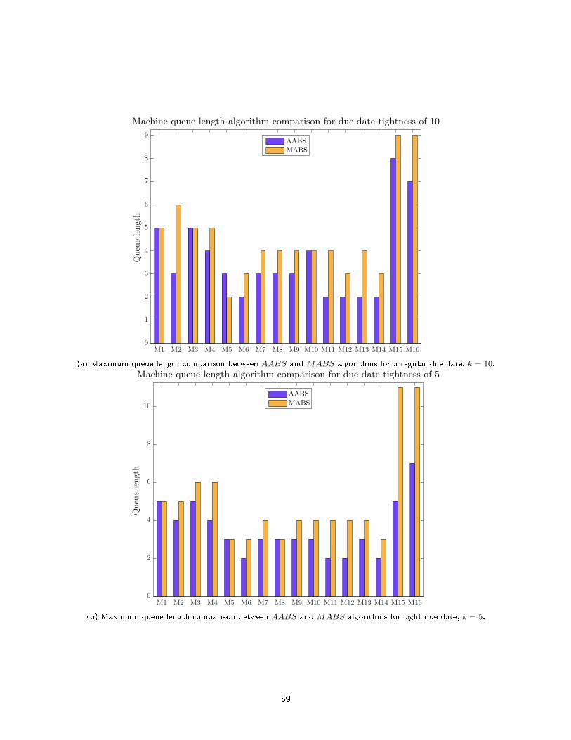
M1 M2 M3 M4 M5 M6 M7 M8 M9 M10 M11 M12 M13 M14 M15 M160

1

2

3

4

5

6

7

8

9Queuelength

Machine queue length algorithm comparison for due date tightness of 10

AABS

MABS

(a) Maximum queue length comparison between AABS and MABS algorithms for a regular due date, k = 10.

M1 M2 M3 M4 M5 M6 M7 M8 M9 M10 M11 M12 M13 M14 M15 M160

2

4

6

8

10

Queuelength

Machine queue length algorithm comparison for due date tightness of 5

AABS

MABS

(b) Maximum queue length comparison between AABS and MABS algorithms for tight due date, k = 5.

59

M1 M2 M3 M4 M5 M6 M7 M8 M9 M10 M11 M12 M13 M14 M15 M160

2

4

6

8

10

Queuelength

Machine queue length algorithm comparison for due date tightness of 3

AABS

MABS

(c) Maximum queue length comparison between AABS and MABS algorithms for a very tight due date, k = 3.

Figure 25: Maximum queue length comparison between AABS and MABS algorithms when varying duedate tightness factor k.

60

6 Conclusions

The objective of this thesis was to develop tools capable of creating a schedule for a dynamic environment.

To achieve this objective static scheduling algorithms were implemented for a planning phase, and dynamic

reactive methods were implemented and created for a dynamic environment state. For the planning phase

two static algorithms were successfully implemented, a mixed integer linear programming algorithm, MILP ,

and a genetic algorithm, GAJobS, which was then extended with a local search, hGAJobS. To respond

to unpredicted or disruptive events, multi-agent based systems coordinated with ant inspired functions were

chosen. A �rst autonomous architecture was used, AABS, and then it was extended to an innovative mediated

architecture, MABS.

The �rst planning algorithm implemented was the MILP in Matlab 17a. It was tested in simple bench-

mark problems and, although it was able to solve the simpler ones even when shop �exibility was increased,

it was unable to generate solutions in cases with more variables, i.e. when the number of operations and

machines was increased it was not able to �nd a solution. The di�culty to solve very complex problems was

expected due to the combinatorial nature of the FJSP. However, part of this behaviour might be related to

the chosen software. Probably if the MILP would have been implemented in a more mature software for

linear programming, such as IBM 's CPLEX, it would be able to solve the failed test instances.

Because of the di�culties encountered withMILP a meta-heuristic approach was taken by implementing

a genetic algorithm. The implemented genetic algorithm, GAJobS, uses a combination strategies to generate

the initial population and create o�spring. Furthermore a coding scheme that prevents infeasible solutions

was used. After testing GAJobS in benchmarks and comparing it to other published genetic algorithms, the

implemented solution was unable to reach the solution presented in the best algorithms. To try to make it

more competitive, a local search using a variable neighbourhood algorithm was added, creating hGAJobS.

By adding the local search, the solution quality improved resulting in an algorithm that was able to �nd the

optimal solution in three of the ten instances and in three other instances did not reach the optimum by

only one time unit. Moreover, hGAJobS proved to be very consistent when comparing to other algorithm,

achieving in all ten instances the best or second to best solutions. It is likely that with more parameter

adjustment and simulation time, the hGAJobS will be able to �nd the optimum in the ten tested instances.

The multi-agent based systems were both successfully implemented. The autonomous architecture was

tested against a well known benchmark case, the GM truck painting, maximizing throughput. It was able

to reach very good results, only falling behind in the case where very high setup penalties were employed.

However, it showed very promising results, and it is likely that with dynamic parameter adjustment it will be

able to highly improve its results. Finally, MABS was tested against AABS in a study-case whose objective

was to minimize maximum lateness. MABS proved to be a less nervous algorithm and showed results that,

although in some metrics were worse than AABS, where much better in light of its objective.

To conclude, two static and two dynamic scheduling algorithms were implemented. All algorithms were

61

successful but they all showed some limitations that are only relevant considering the application. For

instance, for a very small stable plant that has very high processing times, a MILP might be the right choice.

On the other hand, if the plant is very dynamic with constant new order arrival and cancellations, the multi-

agent approach might be indicated. And maybe for high demand plant that has sporadic critical disruptive

events, the combination of a genetic algorithm, such as hGAJobs, and a dynamic reacting algorithm,MABS,

is likely to be the best solution.

6.1 Future Work

While the demonstrated results were good some improvements still need to be made to achieve higher quality

solutions and reach a state where the proposed tools can be implemented successfully in a real dynamic

system.

The genetic algorithm, hGAJobs, although it showed good quality solutions, they could be improved by,

in variable neighbourhood search moving three operations at a time. However, the drawback might be that

for very large problem, it might be too computationally expensive.

The Multi-agent Based systems are very promising algorithms once they can react very fast and with

reasonable solutions, specially MABS. It would be very interesting to see how MABS would behave with

dynamic parameter adjustment based in the current plant state. Results would most certainly improve, yet

the computational burden of the parameter function might take one of the big advantages of the algorithm,

its rapid response.

Finally, exploring the combination of hGAJobS and MABS in a hybrid predictive-reactive scheduling

algorithm.

62

7 References

[1] M. Rüÿmann, M. Lorenz, P. Gerbert, M. Waldner, J. Justus, P. Engel, and M. Harnisch, �Industry 4.0:

The future of productivity and growth in manufacturing industries,� Boston Consulting Group, vol. 9,

2015.

[2] J. Lee, B. Bagheri, and H.-A. Kao, �A cyber-physical systems architecture for industry 4.0-based man-

ufacturing systems,� Manufacturing Letters, vol. 3, pp. 18�23, 2015.

[3] J. A. DiMasi, H. G. Grabowski, and R. W. Hansen, �Innovation in the pharmaceutical industry: new

estimates of r&d costs,� Journal of health economics, vol. 47, pp. 20�33, 2016.

[4] K. Chakrabarty, �Test scheduling for core-based systems using mixed-integer linear programming,� IEEE

Transactions on computer-aided design of integrated circuits and systems, vol. 19, no. 10, pp. 1163�1174,

2000.

[5] D. Ronen, �Ship scheduling: The last decade,� European Journal of Operational Research, vol. 71, no. 3,

pp. 325�333, 1993.

[6] G. W. Chang, M. Aganagic, J. G. Waight, J. Medina, T. Burton, S. Reeves, and M. Christoforidis,

�Experiences with mixed integer linear programming based approaches on short-term hydro scheduling,�

IEEE Transactions on power systems, vol. 16, no. 4, pp. 743�749, 2001.

[7] H. Morais, P. Kadar, P. Faria, Z. A. Vale, and H. Khodr, �Optimal scheduling of a renewable micro-grid

in an isolated load area using mixed-integer linear programming,� Renewable Energy, vol. 35, no. 1, pp.

151�156, 2010.

[8] H. Lee, J. M. Pinto, I. E. Grossmann, and S. Park, �Mixed-integer linear programming model for re�nery

short-term scheduling of crude oil unloading with inventory management,� Industrial & Engineering

Chemistry Research, vol. 35, no. 5, pp. 1630�1641, 1996.

[9] M. Pinedo, Planning and scheduling in manufacturing and services. Springer, 2005, vol. 24.

[10] M. R. Garey, D. S. Johnson, and R. Sethi, �The complexity of �owshop and jobshop scheduling,� Math-

ematics of operations research, vol. 1, no. 2, pp. 117�129, 1976.

[11] P. Fattahi and A. Fallahi, �Dynamic scheduling in �exible job shop systems by considering simultaneously

e�ciency and stability,� CIRP Journal of Manufacturing Science and Technology, vol. 2, no. 2, pp. 114�

123, 2010.

[12] G. E. Vieira, J. W. Herrmann, and E. Lin, �Rescheduling manufacturing systems: a framework of

strategies, policies, and methods,� Journal of scheduling, vol. 6, no. 1, pp. 39�62, 2003.

63

[13] D. Ouelhadj and S. Petrovic, �A survey of dynamic scheduling in manufacturing systems,� Journal of

scheduling, vol. 12, no. 4, pp. 417�431, 2009.

[14] P. Kumar, �Scheduling manufacturing systems of re-entrant lines,� in Stochastic Modeling and Analysis

of Manufacturing Systems. Springer, 1994, pp. 325�360.

[15] W. J. Hopp and M. L. Spearman, Factory physics. Waveland Press, 2011.

[16] S. L. Janak, C. A. Floudas, J. Kallrath, and N. Vormbrock, �Production scheduling of a large-scale

industrial batch plant. ii. reactive scheduling,� Industrial & engineering chemistry research, vol. 45,

no. 25, pp. 8253�8269, 2006.

[17] D. Gupta, C. T. Maravelias, and J. M. Wassick, �From rescheduling to online scheduling,� Chemical

Engineering Research and Design, vol. 116, pp. 83�97, 2016.

[18] P. Brucker and R. Schlie, �Job-shop scheduling with multi-purpose machines,� Computing, vol. 45, no. 4,

pp. 369�375, 1990.

[19] E. Kondili, C. Pantelides, and R. Sargent, �A general algorithm for short-term scheduling of batch

operations�i. milp formulation,� Computers & Chemical Engineering, vol. 17, no. 2, pp. 211�227, 1993.

[20] N. Shah, C. Pantelides, and R. Sargent, �A general algorithm for short-term scheduling of batch op-

erations�ii. computational issues,� Computers & Chemical Engineering, vol. 17, no. 2, pp. 229�244,

1993.

[21] M. Ierapetritou and C. Floudas, �E�ective continuous-time formulation for short-term scheduling. 1.

multipurpose batch processes,� Industrial & engineering chemistry research, vol. 37, no. 11, pp. 4341�

4359, 1998.

[22] J. P. Vin and M. G. Ierapetritou, �A new approach for e�cient rescheduling of multiproduct batch

plants,� Industrial & engineering chemistry research, vol. 39, no. 11, pp. 4228�4238, 2000.

[23] J. M. Novas and G. P. Henning, �Reactive scheduling framework based on domain knowledge and con-

straint programming,� Computers & Chemical Engineering, vol. 34, no. 12, pp. 2129�2148, 2010.

[24] M. Yamamoto and S. Nof, �Scheduling/rescheduling in the manufacturing operating system environ-

ment,� International Journal of Production Research, vol. 23, no. 4, pp. 705�722, 1985.

[25] S. V. Mehta, �Predictable scheduling of a single machine subject to breakdowns,� International Journal

of Computer Integrated Manufacturing, vol. 12, no. 1, pp. 15�38, 1999.

[26] C. Rajendran and O. Holthaus, �A comparative study of dispatching rules in dynamic �owshops and

jobshops,� European journal of operational research, vol. 116, no. 1, pp. 156�170, 1999.

64

[27] P. Brandimarte, �Routing and scheduling in a �exible job shop by tabu search,� Annals of Operations

research, vol. 41, no. 3, pp. 157�183, 1993.

[28] P. Brucker and J. Neyer, �Tabu-search for the multi-mode job-shop problem,� OR Spectrum, vol. 20,

no. 1, pp. 21�28, 1998.

[29] L. Gambardella and M. Mastrolilli, �E�ective neighborhood functions for the �exible job shop problem,�

Journal of scheduling, vol. 3, no. 3, pp. 3�20, 1996.

[30] R. J. M. Vaessens, E. H. Aarts, and J. K. Lenstra, �Job shop scheduling by local search,� INFORMS

Journal on Computing, vol. 8, no. 3, pp. 302�317, 1996.

[31] J. Dorn, R. Kerr, and G. Thalhammer, �Reactive scheduling: Improving the robustness of schedules and

restricting the e�ects of shop �oor disturbances by fuzzy reasoning,� International Journal of Human-

Computer Studies, vol. 42, no. 6, pp. 687�704, 1995.

[32] W. Xia and Z. Wu, �An e�ective hybrid optimization approach for multi-objective �exible job-shop

scheduling problems,� Computers & Industrial Engineering, vol. 48, no. 2, pp. 409�425, 2005.

[33] M. Zweben, E. Davis, B. Daun, and M. J. Deale, �Scheduling and rescheduling with iterative repair,�

IEEE Transactions on Systems, Man, and Cybernetics, vol. 23, no. 6, pp. 1588�1596, 1993.

[34] B. Çali³ and S. Bulkan, �A research survey: review of ai solution strategies of job shop scheduling

problem,� Journal of Intelligent Manufacturing, vol. 26, no. 5, pp. 961�973, 2015.

[35] C. Bierwirth and D. C. Mattfeld, �Production scheduling and rescheduling with genetic algorithms,�

Evolutionary computation, vol. 7, no. 1, pp. 1�17, 1999.

[36] H. Chen, J. Ihlow, and C. Lehmann, �A genetic algorithm for �exible job-shop scheduling,� in Robotics

and Automation, 1999. Proceedings. 1999 IEEE International Conference on, vol. 2. IEEE, 1999, pp.

1120�1125.

[37] N. B. Ho and J. C. Tay, �Genace: An e�cient cultural algorithm for solving the �exible job-shop

problem,� in Evolutionary Computation, 2004. CEC2004. Congress on, vol. 2. IEEE, 2004, pp. 1759�

1766.

[38] I. Kacem, S. Hammadi, and P. Borne, �Approach by localization and multiobjective evolutionary opti-

mization for �exible job-shop scheduling problems,� IEEE Transactions on Systems, Man, and Cyber-

netics, Part C (Applications and Reviews), vol. 32, no. 1, pp. 1�13, 2002.

[39] F. Pezzella, G. Morganti, and G. Ciaschetti, �A genetic algorithm for the �exible job-shop scheduling

problem,� Computers & Operations Research, vol. 35, no. 10, pp. 3202�3212, 2008.

65

[40] G. Zhang, L. Gao, and Y. Shi, �An e�ective genetic algorithm for the �exible job-shop scheduling

problem,� Expert Systems with Applications, vol. 38, no. 4, pp. 3563�3573, 2011.

[41] J. Gao, L. Sun, and M. Gen, �A hybrid genetic and variable neighborhood descent algorithm for �exible

job shop scheduling problems,� Computers & Operations Research, vol. 35, no. 9, pp. 2892�2907, 2008.

[42] G. Chryssolouris and V. Subramaniam, �Dynamic scheduling of manufacturing job shops using genetic

algorithms,� Journal of Intelligent Manufacturing, vol. 12, no. 3, pp. 281�293, 2001.

[43] A. Rossi and G. Dini, �Dynamic scheduling of fms using a real-time genetic algorithm,� International

Journal of Production Research, vol. 38, no. 1, pp. 1�20, 2000.

[44] S. D. Wu, R. H. Storer, and P.-C. Chang, �A rescheduling procedure for manufacturing systems under

random disruptions,� in New directions for operations research in manufacturing. Springer, 1992, pp.

292�306.

[45] A. Rossi and G. Dini, �Flexible job-shop scheduling with routing �exibility and separable setup times

using ant colony optimisation method,� Robotics and Computer-Integrated Manufacturing, vol. 23, no. 5,

pp. 503�516, 2007.

[46] P. Surekha and S. Sumathi, �Solving fuzzy based job shop scheduling problems using ga and aco,� 2010.

[47] K.-L. Huang and C.-J. Liao, �Ant colony optimization combined with taboo search for the job shop

scheduling problem,� Computers & operations research, vol. 35, no. 4, pp. 1030�1046, 2008.

[48] C. A. Silva, J. Sousa, and T. A. Runkler, �Rescheduling and optimization of logistic processes using ga

and aco,� Engineering Applications of Arti�cial Intelligence, vol. 21, no. 3, pp. 343�352, 2008.

[49] C. A. Silva, J. Sousa, T. Runkler, and R. Palm, �Soft computing optimization methods applied to logistic

processes,� International Journal of Approximate Reasoning, vol. 40, no. 3, pp. 280�301, 2005.

[50] W. Shen, D. H. Norrie, and J.-P. Barthès, Multi-agent systems for concurrent intelligent design and

manufacturing. CRC press, 2003.

[51] W. Shen, �Distributed manufacturing scheduling using intelligent agents,� IEEE intelligent systems,

vol. 17, no. 1, pp. 88�94, 2002.

[52] W. Xiang and H. P. Lee, �Ant colony intelligence in multi-agent dynamic manufacturing scheduling,�

Engineering Applications of Arti�cial Intelligence, vol. 21, no. 1, pp. 73�85, 2008.

[53] N. R. Jennings, �On agent-based software engineering,� Arti�cial intelligence, vol. 117, no. 2, pp. 277�

296, 2000.

[54] R. Smith, �Communication and control in problem solver,� IEEE Transactions on computers, vol. 29,

no. 12, pp. 1104�1113, 1980.

66

[55] M. Shaw, �Distributed planning in cellular �exible manufacturing systems,� INFOR: Information Sys-

tems and Operational Research, vol. 25, no. 1, pp. 13�25, 1987.

[56] T. W. Sandholm, �Automated contracting in distributed manufacturing among independent companies,�

Journal of Intelligent Manufacturing, vol. 11, no. 3, pp. 271�283, 2000.

[57] V. A. Cicirello and S. F. Smith, �Insect societies and manufacturing,� in The IJCAI-01 Workshop on

Arti�cial Intelligence and Manufacturing: New AI Paradigms for Manufacturing, 2001, pp. 33�38.

[58] ��, �Wasp-like agents for distributed factory coordination,� Autonomous Agents and Multi-agent sys-

tems, vol. 8, no. 3, pp. 237�266, 2004.

[59] R. Morley, �Painting trucks at general motors: The e�ectiveness of a complexity-based approach,� Em-

bracing Complexity: Exploring the application of complex adaptive systems to business, pp. 53�58, 1996.

[60] L. Meyyappan, C. Saygin, and C. H. Dagli, �Real-time routing in �exible �ow shops: a self-adaptive

swarm-based control model,� International Journal of Production Research, vol. 45, no. 21, pp. 5157�

5172, 2007.

[61] M. Dorigo and L. M. Gambardella, �Ant colonies for the travelling salesman problem,� BioSystems,

vol. 43, no. 2, pp. 73�81, 1997.

[62] V. A. Cicirello and S. F. Smith, �Ant colony control for autonomous decentralized shop �oor routing,� in

Autonomous Decentralized Systems, 2001. Proceedings. 5th International Symposium on. IEEE, 2001,

pp. 383�390.

[63] C. A. Floudas and X. Lin, �Mixed integer linear programming in process scheduling: Modeling, algo-

rithms, and applications,� Annals of Operations Research, vol. 139, no. 1, pp. 131�162, 2005.

[64] C. Pach, T. Berger, T. Bonte, and D. Trentesaux, �Orca-fms: a dynamic architecture for the optimized

and reactive control of �exible manufacturing scheduling,� Computers in Industry, vol. 65, no. 4, pp.

706�720, 2014.

[65] F. Werner, �Genetic algorithms for shop scheduling problems: a survey,� Preprint, vol. 11, p. 31, 2011.

[66] K.-M. Lee, T. Yamakawa, and K.-M. Lee, �A genetic algorithm for general machine scheduling prob-

lems,� in Knowledge-Based Intelligent Electronic Systems, 1998. Proceedings KES'98. 1998 Second In-

ternational Conference on, vol. 2. IEEE, 1998, pp. 60�66.

[67] J. Hurink, B. Jurisch, and M. Thole, �Tabu search for the job-shop scheduling problem with multi-

purpose machines,� Operations-Research-Spektrum, vol. 15, no. 4, pp. 205�215, 1994.

[68] R. Storn and K. Price, �Di�erential evolution � a simple and e�cient heuristic for global optimization

over continuous spaces,� Journal of Global Optimization, vol. 11, no. 4, pp. 341�359, Dec 1997. [Online].

Available: https://doi.org/10.1023/A:1008202821328

67

[69] I. Driss, K. N. Mouss, and A. Laggoun, �A new genetic algorithm for �exible job-shop scheduling prob-

lems,� Journal of mechanical science and technology, vol. 29, no. 3, p. 1273, 2015.

68