FasTraCra “When too much schedule compression leads to explosion”

SCHEDULE COMPRESSION OF AN URBAN
HIGHWAY PROJECT USING THE LINEAR
SCHEDULING METHOD
Ibrahim Tarkan Yuksel and James T. O'Connor
CENTER FOR TRANSPORTATION RESEARCH BUREAU OF ENGINEERING RESEARCH THE UNIVERSITY OF TEXAS AT AUSTIN
FEBRUARY 2000

SCHEDULE COMPRESSION OF AN URBAN HIGHWAY PROJECT USING THE LINEAR SCHEDULING METHOD
by
Ibrahim Tarkan Yuksel
and
James T. O'Connor, Ph.D.
Center for Transportation Research
The University of Texas at Austin
3208 Red River, Ste. 200
Austin, Texas 78705
February 2000

ii

This is the third report published from work conducted by the Center for
Transportation Research in partnership with the Dallas District of the Texas Department of
Transportation since 1994 through Cooperative Research Program Study 7-2922 and
Interagency Contracts 96-0017, 98-0003, and 00-0027.
ACKNOWLEDGEMENTS
The authors wish to express their appreciation for the support and contributions to
this work from Makrameh Gataineh, Project Manager for the Texas Department of
Transportation, Lyle Clark, Project Engineer for Granite Construction Company, James Hill,
Construction Inspector for the Texas Department of Transportation, and Nabeel Khwaja,
Research Engineer with the Center for Transportation Research at The University of Texas at
Austin.
iii

IV

ABSTRACT
Traditional network scheduling methods such as Critical Path Method (CPM),
Program Evaluation and Review Techniques (PERT), and bar charting are generally
considered to be less effective for the planning of linear projects due to the cumbersome way
in which they model repetitive activities. The literature indicates that linear scheduling
techniques are more suitable to manage linear projects such as highways and tunnels. Linear
scheduling is a practical tool that can be utilized for developing and maintaining the
construction schedule as well as for seeking alternative schedules to the existing schedule.
Coupling the strong visual advantage(s) and flexibility of this technique with a systematic
approach, the construction schedule may be compressed without major cost impacts.
v

TABLE OF CONTENTS
ABSTRACT v
CHAPTER 1. INTRODUCTION 1
Background .......................................................................................................................... 1 Research Objectives ............................................................................................................ 2 Research Motive .................................................................................................................. 2 Scope Limitations ............................................................................................................... .4 Report Structure ................................................................................................................... 4
CHAPTER 2. STUDY METHODOLOGY 7
Overview ............................................................................................................................. .7 Familiarization with the Highway Project and Research Objectives ............................... 8 Literature Review for the Study ........................................................................................ .9 Formulating Study Approach .......................................................................................... .10 Data Collection Plan and Execution ................................................................................ .10 Application of the LSM for Schedule Compression ...................................................... .11 Presentation, Evaluation, and Refinement of Recommendations ................................. .12 Proposed Schedule for the Critical Area .......................................................................... 13
CHAPTER 3. PROJECT DESCRIPTION AND LITERATURE REVIEW 15
Proj ect Description ............................................................................................................ 15 Literature Review on Schedule Compression ................................................................ .16 Literature Review on the LSM 19
CHAPTER 4. SCHEDULE COMPRESSION ANALYSIS FOR NORTH CENTRAL EXPRESSWAY (NCE) SI 33
Overview ............................................................................................................................ 33 WBS for the Critical Area ................................................................................................. 33 The As-Planned Linear Schedule 36 Proposed Schedule Compression Changes .................................................................... ..41 Anticipated Cost Impact of Proposed Changes ............................................................. ..45 Proposed Schedule ............................................................................................................ .46 Responses to Proposed Changes .................................................................................... ..47 Analysis of Responses ...................................................................................................... .47 Recommended construction Schedule Compression Analysis Method ....................... ..48
vi

CHAPTER 5. CONCLUSIONS AND RECOMMENDATIONS 51
Cone I usions _______________________________________________________________________________________________________________________ 51 Recommendations _____________________________________________________________________________________________________________ 5 2
BIBLIOGRAPHY 55
Appendix A: As-Planned Linear Schedule. __________________________________________________________________________ 57 Appendix B: Schedule With Proposed Change #1 ______________________________________________________________ 63 Appendix C: Schedule With Proposed Change #2 ______________________________________________________________ 67 Appendix D: Schedule With Proposed Change #3 _____________________________________________________________ ) 1 Appendix E: Schedule With Proposed Change #8. _____________________________________________________________ )5 Appendix F: Proposed Linear Schedule for Review __________________________________________________________ )9 Appendix G: Schedule Compression Questionnaire ___________________________________________________________ 85 Appendix H: Linear Schedule With Approved Changes. ____________________________________________________ 89
vii

V111

CHAPTERl.
INTRODUCTION
BACKGROUND
The term "schedule" is defined as "the plan for completion of a project based on a
logical arrangement of activities" (Popescu and Charoenngam, 1994). Basically, a schedule
consists of activities or tasks that will be performed during a project. The number of
activities in a schedule usually depends on the size of the project as well as the selected level
of detail. One should expect a schedule to become more complicated as the number of
activities increase. A schedule is used as a means to:
a. communicate a project plan to various project participants,
b. control and project, and
c. provide management with project information for decision-making (Popescu and
Charoenngam, 1994).
Several different scheduling methods, such as color graphs, percentage of completion,
line of balance, linear scheduling, bar charts, and Program Evaluation and Review
Techniques (PERT) have been implemented on different types of projects. Today, Critical
Path Method (CPM), developed in the early 1960s, is the most widely used project method
(Popescu and Charoenngam, 1994). The CPM schedule method involves a network diagram
to portray the interrelationships among activities. The CPM method uses a mathematical
procedure to calculate the project schedule based on the estimated duration of each activity
and the assumed dependencies among the activities (Parvin and Vorster, 1993). This
procedure is referred to as "network calculation."
Selecting the appropriate scheduling method is essential to achieving the
aforementioned objectives of scheduling. The specific type of schedule to be used should be
commensurate with the needs of the project. The question of whether CPM is the answer for
linear projects such as pipelines, tunneling, and highway construction still remains
unanswered. This report presents an application of an alternative scheduling method, the
1

Linear Scheduling Method (LSM), on an urban highway project for the specific task of
construction schedule compression. The advantages that this method offers for linear type
projects are discussed, along with other findings.
RESEARCH OBJECTIVES
The objectives of this research are to:
a. understand the principles of the LSM,
b. implement the method on an urban highway project as a schedule compression
technique, and
c. analyze the effectiveness and appropriateness of the method for this purpose on
this type of project.
RESEARCH MOTIVE
Today's urban highway construction projects are more complicated than those of the
past. Projects are often constructed in close proximity to traffic and the public, increasing the
importance of time for constructing a project. In many building projects, cost is the main
driver behind the execution of the project. In contrast, urban highway projects typically
emphasize time over cost in order to mitigate the risks associated with this public
endangering type of construction. The factors that motivated this schedule compression
study and the selection of the method can be summarized under two major headings: generic
factors and project-specific factors.
Generic Factors
The use of the LSM has been recommended to highway contractors for greater
management and control of the work and to prove or disprove delay claims and extension
requests (Parvin, 1990). It allows for a better understanding of the linear project than any
other scheduling technique, primarily because the scheduler has access to activities' rates of
production as well as the location (Arditi and Albulak, 1986). These attributes made
application of the LSM well suited to the North Central Expressway (NCE) project.
2

The CPM is a useful tool for projects where there are strict dependencies and
constraints between project activities, such as the construction of a building. For example, it
is impossible to form the first floor deck of a building before foundation slab is poured and
columns and beams are formed. However, there are fewer such clear dependencies in
repetitive projects such as highway construction. The contractor has more options, such as
constructing a bridge before constructing the main lanes underneath, or vice versa.
Therefore, the project management team often has greater latitude to deviate from the initial
construction schedule during the course of the project. The purpose of the deviation may
either be schedule compression, as in this study, or achieving better constructability. The
LSM was selected for its flexibility, which was needed to seek the alternative schedules.
Project-Specific Factors
The NCE has been a key link in Dallas' transportation network for over 45 years. At
the start of the reconstruction project, traffic volumes on the NCE averaged 150,000 vehicles
per day (Tyer and Krammes, 1993). Due to this heavy traffic load, early project completion
was desired.
The reconstruction of the NCE started in 1990 with the northern section, termed
North 1 (Nl). Since that time, the public has been impacted by various stages of
construction. In order to mitigate these adverse impacts, two decisions were made by the
project stakeholders. First, a strong relationship was forged between contractors for various
project segments and the Texas Department of Transportation (TxDOT) to address mitigation
needs. Second, a North Central Mobility Task Force (NCMTF) was formed to address issues
of mobility planning, traffic management, public information, and community outreach. Of
course, early completion of the project would provide the ultimate relief to the public.
The contract between TxDOT and the contractor stipulated the use of Primavera
Project Planner as the scheduling software. That decision established CPM as the scheduling
method. The baseline schedule that was submitted to TxDOT consisted of more than 3,000
activities and even more activity relationships. Due to the complexity of the project, the
updated CPM schedule did not reflect the current status of the project with enough precision
3

to conduct a schedule compression study. This situation indicated that the schedule
compression study might benefit from an alternative technique.
SCOPE LIMITATIONS
The scope of the study was limited to the analysis of the construction schedule
compression of a selected project from TxDOT using the LSM. The following list elaborates
on the scope definition of the selected project.
a. The selected construction project had only one and one-half years remaining out
of an estimated five-year construction schedule when this study was initiated.
There were three areas (segments) available to choose for this study. The 1,400-
foot segment between station markers 71 and 85 was selected because it was the
last· area to be constructed. Thus, schedule compression would affect the project
completion date.
b. A schedule that reflected the project team's plan was developed for the selected
segment using the LSM. Schedule compression techniques were applied to the
developed schedule to achieve the proposed schedule changes. For the same
reason, engineering phase methods, procurement phase methods, and contractual
methods used for schedule compression were not addressed this study.
c. Project management staffing methods, which deal with the way the employees are
managed, were not included in the study scope to prevent interference with the
internal procedures of the owner and/or contractor.
d. Economic impacts of proposed changes were not assessed in this study.
Nevertheless, some suggestions were eliminated during the refinement process
due to their obvious cost impacts.
REPORT STRUCTURE
The research methodology is explained in Chapter 2 and details the approach taken to
solve the specific problem of schedule compression. The overall methodology that was
4

followed is provided in the first section. Then each step is expanded, displaying the activities
involved and the outcomes from the related major steps.
Chapter 3 includes the literature review and project description. Past research efforts
relevant to this study are summarized in the literature review section. A detailed definition
and the principles of the LSM are also presented in that section for readers who are not
familiar with the method. A detailed description of the selected project for the study is
provided in the second part of the chapter. The report is organized so that readers will be
familiar with the selected project and the utilized method prior to Chapter 4.
Chapter 4 details the schedule compression analysis and techniques utilized
throughout the study. Collected data and analysis results are presented in the chapter, as well
as the contractor's recommended compression tactics. Construction Schedule Compression
Analysis Method, which is reflective of lessons learned, is presented for consideration on
future projects.
Finally, Chapter 5 summarizes research conclusions and provides recommendations.
5

6

CHAPTER 2.
STUDY METHODOLOGY
OVERVIEW
The methodology that was followed to complete this study is presented in this
chapter. After providing a brief overview of the methodology, each major step is expanded
to display the activities performed and the resulting output that becomes the input for the
next step.
Familiarization with highway project and research objectives
~ Literature review on
schedule compression and scheduling methods
~ Formulation of study approach
! Data collection
plan and execution
~ Application of Linear
Scheduling Method for compression
! Presentation, evaluation
and refinement of recommendations
! Final schedule diagrams
for critical area
Figure 2.1. Study Methodology
7

Figure 2.1 illustrates the approach taken in this study. The specific steps followed
included: familiarization with the highway project and research objectives; literature review;
formulation of study approach; data collection; application of the LSM; presentation,
evaluation and refinement of the recommendations; and presentation of proposed schedule
diagrams for the critical area.
FAMILIARIZATION WITH THE HIGHWAY PROJECT AND RESEARCH
OBJECTIVES
An understanding of the objectives was essential to the success of the study. Several
meetings were conducted with the project team to ensure that study objectives were aligned
with their expectations. These meetings were also useful in obtaining the stakeholders'
approval and in creating the team environment for the study.
Due to the complexity of the project, becoming familiar with the highway project
took longer than expected. Suggesting valuable alternatives to the existing schedule required
that the construction logic in place be thoroughly understood. Analyzing the construction
plans was the first activity undertaken. Slight differences between the plans and the actual
field progress were clarified through meetings with TxDOT's project manager. Several site
visits were conducted with the guidance of TxDOT inspectors. The next step was to analyze
the baseline CPM schedule to better understand the construction sequence that was initially
planned for the project as a whole.
As a result of these activities, study scope and objectives were documented. Figure
2.2 summarizes the activities and the outcome for this step.
8

MAJOR STEP
Familiarization with highway project and research objectives
ACTIVITIES
Conduct meetings with project team
Analyze the plans
Analyze the schedule
Perform site visits
OUTCOME
Objectives
Scope
Project Details
Figure 2.2. Familiarization Activities and Outcome
LITERATURE REVIEW FOR THE STUDY
A review of published literature provided background on the LSM and schedule
compression strategies through a number of articles, books, journal papers, and Web pages,
which were useful and informative. Lack of awareness of the LSM within the construction
industry is reflected in the small number of studies that have been conducted in that field.
After completing analysis of related previous studies, compression strategies were identified
along with the scheduling technique to be utilized for the study. Figure 2.3 summarizes the
activities and outcome for this step.
MAJOR STEP
Literature review on schedule compression
and scheduling methods
ACTIVITIES
Analyze related previous studies
Figure 2.3. Literature Review for the Study
9
OUTCOME
Compression strategies
Linear Scheduling Method as method for study

FORMULATING STUDY APPROACH
A linear schedule consists of diagrams showing both the time and location at which a
certain crew will be working on a given operation (Parvin and Yorster, 1993). It is necessary
to cover all areas of a project when the LSM is utilized as the primary method of schedule
maintenance. However, for schedule compression, only critical areas that impact the overall
duration of the project need to be analyzed. In the NeE project, the selected critical area was
the last area to be constructed, which was independent from other areas and relatively easy to
isolate.
After the selection of the critical area, required data were identified to develop the
linear schedule for that area, resulting in the development of the execution plan for the study.
Figure 2.4 summarizes the activities and the outcome for this step.
MAJOR STEP
Formulating study approach
ACTIVITIES
Select critical area
1 Identify needs for data
Figure 2.4. Formulating Study Approach
DATA COLLECTION PLAN AND EXECUTION
OUTCOME
Study execution plan
Many changes had occurred following the approval of the baseline schedule;
therefore it was necessary to develop a new schedule containing the planned activities for the
selected critical area. First, a Work Breakdown Structure (WBS)-a task-oriented family
tree of work activities to be accomplished-was developed with the help of the contractor.
The next step was to create an activity list along with work quantities and anticipated
production rates of the crews. The activity list was derived from the work items of the WBS.
Meetings were held with the contractor's project engineer to assure that the developed
activity list matched the project team's plan. Anticipated crew production rates were either
obtained from past records or through interviews with the contractor's foremen. Upon
10

completion of the activity list, needed resources by activity were identified through meetings
with the contractor's field engineers and superintendents. The accumulated data were
organized and a Linear Schedule Diagram (as planned) for the critical area was drawn.
Figure 2.5 summarizes the activities and the outcome for this step.
MA.JORSTEP
Data collection plan and execution
ACTIvITIES
Create Work Breakdown Structure (WBS)
~ Create the activity list
along with quantities of work and production rates
~ Identify allocated
resources
! Identify planned
construction sequence
Figure 2.5. Data Collection Plan and Execution
OUTCOME
Linear schedule diagram for the critical area
(as planned)
APPLICATION OF THE LSM FOR SCHEDULE COMPRESSION
Schedule compression strategies identified in earlier steps were applied to the
activities of the as-planned linear schedule, and proposed changes were developed
accordingly. The activities and the outcome of this step are shown in Figure 2.6.
11

MAJOR STEP
Application of Linear Scheduling Method for schedule compression
ACTIVITIES
Overlapping activities
Increasing utilization (overtime)
Implementing night work
! Adding resources
1 Modifying technology
used
1 Modifying construction
logic
QlJTCOME
Suggestions for schedule compression
Figure 2.6. Application of the LSM for Schedule Compression
PRESENTATION, EVALUATION, AND REFINEMENT OF RECOMMENDATIONS
A final meeting was scheduled with TxDOT's project manager and the contractor's
project engineer to refine the proposed changes and to select those with the greatest potential
for implementation. Some of the proposed changes were eliminated due to issues such as
safety concerns (for example, TxDOT did not allow the contractor to work at night) and lack
of additional resources (cost impact). The activities and the outcome of this step are shown
in Figure 2.7.
MAJOR STEP
Presentation, evaluation, and refinement of recommendations
ACTIVITIES
Schedule final meeting with project team
QlJTCOME
Refined ideas with greatest potential for
implementation
Figure 2.7. Presentation, Evaluation, and Refinement of Recommendations
12

PROPOSED SCHEDULE FOR THE CRITICAL AREA
Refined proposed changes formed the basis for the final step of the study. The
anticipated impact of the proposed changes was characterized by comparing the as-planned
linear schedule to the modified suggested linear schedule, which was impacted by the
particular proposed change.
After characterizing the anticipated impact of each proposed change, the proposed
schedule for the critical area was developed by utilizing those proposed changes that would
give the best schedule compression solution. Comparison and elimination of proposed
changes were performed in cases where the impact of one proposed change could make
another proposed change less effective if applied together. More details are provided in
Chapter 4.
After submitting the final report to the project team, a concluding questionnaire was
developed to obtain contractor feedback on the actual application of the proposed changes.
Figure 2.8 summarizes the activities and the outcome of this step.
MA.JORSTEP
Final schedule diagrams for the critical area
ACTIVITIES
Compare planned schedule with suggested schedule
for each suggestion
~ Draw suggested final schedule
1 Get feedback from
contractor organization
OUTCOME
Anticipated impact of each suggestion
if applied
Anticipated impact of compression on the
overall schedule
Study evaluation
Figure 2.8. Proposed Schedule for the Critical Area
13

14

CHAPTER 3.
PROJECT DESCRIPTION AND LITERATURE REVIEW
PROJECT DESCRIPTION
The NCE lies in the heart of Dallas, linking Dallas' central business district (CBD)
with the major urban and suburban areas of North Dallas. Almost 25 percent of the office
space in Dallas lies in the CBD and the NCE business district.
Originally designed in the late 1940's and built in the early 1950's as one of the most
extravagant public infrastructure development projects of its time, it became synonymous
with the economic growth of the City of Dallas. It was designed to cater to the traveling
needs of 75,000 vehicles per day, and reached its capacity in the early 1970's. For the next
decade or so, it went through a period of reconstruction design development. The final
design included depressing the main lanes by almost 25 feet in tight right-of-way (ROW)
areas, with cantilevered frontage roads overhanging the main lanes. The circumstances
associated with this plan presented challenges to project designers and constructors. The
three major highlights of this reconstruction project were:
a. construction of user-friendly, extra wide bridges,
b. construction of cantilevered frontage roads, and
c. traffic control during the ten-year reconstruction process.
The nine-mile stretch of the NCE was divided into five individual projects to improve
manageability, with each project being less than two miles in length. From LBJ Freeway (at
the northern end) to Woodall Rodgers (at the southern end), the reconstructed freeway would
have four lanes (increased from two) in both directions with continuous frontage roads and
cross-street bridges above the main lanes. The five individual projects were named North 1
(Nl), North 2 (N2), Middle (M), South 2 (S2), and South 1 (SI). The scope of this study was
limited to a segment of the SI project that connects Woodall Rodgers and IH-45 at the south
end with the S2 project limits at the north end (see Figure 3.1). At an estimated cost of $110
million, reconstruction of the NCE is one of the largest projects in TxDOT's history.
15

t FOREST N------f I
ROYAL
@) (1.3 miles)
WALNUT HILL
NORTHWEST HWY 5i
SOUTHWESTERN
LOVERS
MONTICELLO --------- --------------FITZHUGH
LEMMON
WOODALL RODGERS
(2.4 miles)
Approximate Project Boundaries
Figure 3.1. NCE Project Sections
LITERATURE REVIEW ON SCHEDULE COMPRESSION
In their 1989 review, Antill and Woodhead described network compression as the
expediting of an activity or a group of activities by utilizing additional resources. They
stated that this expediting is dependent only on the availability of resources, the form of
utility data curves, and the desire to speed up project completion. They defined the utility
data curve as the curve showing the relationship between direct cost and time of completion
16

for each of the construction operation~. Sample utility data curves of two activities are shown
in Figure 3.2.
Cost Cost
2000 3200
:~= . 3
, ......... 00
4000 -5000 I
L....-....... _ ...... ____ .... Time L....-_________ ~ Time
Tcrash Tnormal 4 10
Activity A
Tcrash Tnormal 10 20
Activity B
Tcrash: Shprtest possible activity duration Tnormal: <i>ptimum activity duration s= Cost slope
Figure 3.2. ISample Utility Data Curves
Figure 3.2 implies that for activity A (cost slope = 300), the schedule can be crashed
by six days with an additional cost of $1,800. On the other hand, activity B (cost slope =
200) can be crashed by ten days with I an additional cost of $2,000. The optimum solution
would be compressing activity B (wit~ its flatter cost slope). This approach is useful when I
the utility data curves for all activities are available. I
Behrig et al. (1990) provided ~ detailed study on concepts and methods of schedule
compression. They identified schedu~e compression techniques that can be used in one or
more of the engineering, procurement,'1 and construction phases of the project and evaluated I
each technique's impact on the project cost and duration when applied to the three phases of
the project. Accordingly, they addressbd 94 concepts and methods of schedule compression, I
which were grouped under eight major headings, and are as follows.
a. Ideas applicable to all phasfs of a project: These methods can be applied to any
phase of the project. A fe~ examples are "avoidance of interruption," "efficient
17

staffing," and "incorporation of incentives."
b. Engineering phase: These methods are recommended for use in the engineering
phase of the project. A few examples are "change management system during
engineering," "constructability analysis during engineering," and "freezing of
project scope."
c. Contractual approach: These methods are recommended for use prior to the
issuance of contracts and/or subcontracts. A few examples are "fast-track
scheduling," "fair risk assignment," and "minimizing owner involvement."
d. Scheduling: These methods relate to the scheduling phase of the project. A few
examples are "realistic scheduling," "start-up driven scheduling," and "use of
float flexibility."
e. Materials management: These methods address the schedule compression
opportunities that come from better materials management. A few examples are
"just-in-time material deliveries," "dedicated truck shipments," and "product
identification."
f. Construction work management: These methods address the construction
management issues in the field. A few examples are "advanced construction
equipment," "critical equipment contingency planning," and "making site a good
place to work."
g. Field labor management: These methods address the compression opportunities
that come from better field labor management. A few examples are "pre-work
briefings," "crew training and rehearsals," and "labor minimization."
h. Start-up phase: These methods are recommended for use in the start-up phase. A
few examples are "minimizing scope of start-up," "temporary start-up systems,"
and "start-up planning."
Popescu! presented the following techniques to reduce activity duration:
1 C. M. Popescu, Ph.D., Professor of Civil Engineering at The University of Texas at Austin, course notes from 1998 time management course.
18

a. select an alternate technology or production process,
b. allocate more resources if possible,
c. implement overtime schedule, and
e. eliminate/reduce imposed delay(s).
The literature indicates that there are several methods and techniques for schedule
compression. However, the selection of a method requires careful consideration of many
variables. Most importantly, management must consider all the project activities that will be
impacted when the method is applied and predict the possible outcome of the action.
LITERATURE REVIEW ON THE LSM
Origins of the LSM
The exact origins of the LSM are not clear, and indeed there may have been multiple
origins. There is no definitive information as to when linear scheduling techniques were first
used to develop production schedules. Reviewing the available literature, it is apparent that
interpretation and application of the method by researchers followed slightly different paths,
and yet were based on common features: repetitive units of work and known or estimated
rates at which these units are produced.
The LSM has some relationship to the line of balance (LOB) technique, a scheduling
method developed by the U.S. Navy in the early 1950s for industrial manufacturing and
production control. The objective of the LOB technique is to ensure that components or
subassemblies are available at the time they are required to meet the production schedule of
the final assembly. O'Brien (1969) summarized the technique in relation to the scheduling of
manufacturing processes. Three diagrams are used in the LOB technique, as shown in Figure
3.3. A production diagram (Figure 3.3.a) shows the relationship of the assembly operations
for a single unit. An objective diagram (Figure 3.3.b) is used to plot the planned or actual (or
both) number of units produced versus time. A progress diagram (Figure 3.3.c) is prepared
for any particular date of interest during the production process. The progress diagram
shows the number of units for which each of the subassembly operations has been completed.
19

4
/ Jan
6 4&5 3 2
I I
3 2 1 o Months prior to unit completion
(a) Production diagram
/ ~
/ V
V V
70 60
50
40
30
20
10
Feb Mar Apr May Jun Jul 0
1 I Units
D Subcontractor part
o Purchased part
V Subassembly part
6 Unit completion
2 3 4 5 6
(b) Objective diagram (c) Progress diagram for Feb 6
Figure 3.3. Line of Balance Technique Example
20

O'Brien mentioned that the production diagram of LOB is similar to an activity-on
arrow network, except that it is a network showing assembly operations for only one unit of
many produced. The production diagram places primary emphasis on the event ending each
assembly task.
O'Brien compared the progress diagram with the bar chart in his analysis. Prepared
for a particular date, the progress diagram graphs, as a vertical bar for each task, the actual
number of unit tasks completed. Actual progress is compared to the "line of balance," a level
of progress needed on each task at the particular date to achieve the objective. He stated that
the bar chart is different in the sense that it graphs tasks on the vertical axis versus the time
period of activity on the horizontal axis. In his analysis, O'Brien mentioned that the LSM
diagram resembles the objective diagram of the LOB technique in that they both use time as
one axis and some measure of production as the perpendicular axis. However, the objective
diagram, as seen in Figure 3.1.b, is used to schedule or record the cumulative events of unit
completion, whereas the LSM diagram is used to plan or record progress of multiple
activities that are moving continuously in sequence along the length of a single project. In
conclusion, he stated that any differentiation between the LSM and the LOB techniques
might only be a question of emphasis. LSM emphasizes a diagram similar to the objective
diagram for planning purposes, while LOB puts more emphasis on the balance line of the
progress diagram.
Carr and Meyer (1974) applied the LOB technique to construction planning of
repetitive building units. Details of the methods were presented, as well as an examination of
the method in relation to complementary CPM and bar chart methods. Popescu of the
University of Texas at Austin presented a simplified example of the application of the LOB
technique to repetitive building units in his graduate course, Time Management (Figure 3.4).
21

Operation
Rough-in Plumbing _ & Electrical I
I I
Concrete Slab I_
Wood Framing, Door & Windows
I I I I - I
Roof Deck & Felt I
16 14 12 10 8 (a) Setback chart
642 0
Time in Working Days
Dry-in houses
40
30
20
10
Planned Work
/Actualworkperformed . at the data date
./ Month
1 2 3 4 5 (b) Objective chart
Number of Completed Activities From Setback Chart
40
30
20
10
40
34
22 2Q ....................... _ ......... .
Rough-in Conc. Wood Roof Deck Plumbing Slab Framing & Felt
(c) Progress chart
Actual progress at the data date
Figure 3.4. Example of LOB Technique for Construction
The sample project presented in Figure 3.4 encompasses the construction of small,
wood-framed house dry-in operations. The setback chart (Figure 3.4.a) shows the operations
involved in a repetitive project in their proper order. The objective chart (Figure 3.4.b) is
used to schedule the work. It displays the planned number versus completed number of
houses plotted on a time line. The third diagram, the progress chart, shows the number of
22

repetitive activities completed at a specific date (data date). Arditi and Albulak (1986)
addressed the flaws of this method. Specifically, they stated that the method is extremely
sensitive to errors in the activity duration estimates. This attribute dictates that the estimation
of the production rates should be performed with the highest possible precision.
Publications relating the LSM to highway and other transportation projects are more
limited. Spang and Zimmerman (1967) described the construction of a tunnel by using a
Linear Schedule Diagram showing time versus distance along the tunnel for the major
activities. They found that this method improved the communication of schedule
information through visual impact. In his 1981 review, Johnston described a graphical
method that was particularly applicable to linear projects. He foresaw the use of the method
in U. S. highway construction and maintenance projects, adding that the method was
increasingly being used in the Middle East. Recently, several books on construction
management have included brief sections about LSM. However, the reviewed books do not
give many details about the method, and seemingly only intended to inform readers of the
existence of the method.
Principles of the LSM
The LSM can be applied in different forms pursuing different objectives, as discussed
in the previous section. Accordingly, researchers have discussed different sets of principles
in their studies. Parvin and Vorster (1993) presented the principles of the LSM that they
recommend to highway contractors. Those principles will be discussed in this section with a
minor change in the axes selection. Parvin and Vorster represented location with the
horizontal axis and time with the vertical axis. To facilitate the understanding of the method,
the axes will be reversed. In other words, location will be plotted on the vertical axis and
time will be plotted on the horizontal axis, matching the application on the NCE project.
Components of a Linear Schedule
Axes. The x-axis, or the horizontal dimension, is used to measure time. The starting
date of the schedule is located at the leftmost point of the horizontal axis. The time scale is
23

chosen to fit the scope of a particular project. Possible units for measuring time on the x-axis
are working days, calendar days, or weeks. The y-axis, or the vertical dimension, is used to
measure location and distance. Highway projects are linear by nature, allowing locations
along the highway to be visualized as points along the vertical axis of the schedule. Possible
units for measuring distance are feet, stations, miles, meters, or kilometers.
Sight Lines. After defining axes for the linear schedule, additional horizontal and
vertical lines should be drawn to make the diagram easier to read. These sight lines provide
visual guidance between the axes and the area used for drawing the schedule. Vertical lines
correspond to dates in time, whereas horizontal lines correspond to locations. Figure 3.5 is
an example of a linear schedule showing the axes and the sight lines before activities are
plotted.
60
50
,-,. ~
40 .S !S tI) '-' 30 ~ 0 .~ u 0
.....l 20
10
0
----.--~-.-----.~------ .. ~-----.-.---------~---- .. · . · . : . · · · · ·-··---r·-------~--------~------·-~----·---r·----· · " · " · '. I :: · . I I I • I
-------~--------~--------~--------~--------~--.-.-· ., . : · · · · • I • I •
--.----~-.--.---~.-------~-.--.-.-~--.-----~-.---. I I I I I I I I •
• I I I I I. I · · · · .. .
-------~--------~--------~--------~--------~------• • I • I I I • I I .. . : : · . .. . • I • • •
-----.-~--------~--------~--------~--------~------I • I I I
• I I I I .. . .. . .. . .. . .. . 1 2 3
Time (Week)
4 5
Figure 3.5. Axes and Sight Lines of a Linear Schedule
24

Location Details. Representation of important physical features of the project on the
y-axis is a helpful visual aid in the planning process. A simple plan or profile view of the
project can be drawn. Locations of features, such as bridges, culverts, or retaining walls may
be placed on the plan view of the schedule. A project plan is shown along the y-axis in
Figure 3.5. A bridge and a manhole are graphically represented on the plan view. This
illustration strengthens the visual connection achieved between the plan view and the linear
schedule, improving comprehension of the schedule.
Indication of constraints. Conditions may exist on a project that prohibit work from
taking place in certain locations at certain times. Linear scheduling techniques can display
access restrictions on the schedule to provide a visual reminder that an area is unavailable.
Examples of access constraints are shown in Figure 3.6. The section between stations 0 and
60 is marked as "Weather Constraint" for the month of December. Similarly, the section
between stations ten and 30 is marked as "Access not available" for the first two weeks of
February.
, , , , , Manh~le
0'
60 r-- ...... ~ ...........................•...• ~ ........ ~ .... .
I :~:~:~:~:~:~:~:~ ~ ~
50 - ....... ~ ....•... ~l~l~l~l~l~l~l~l········~········}· ... . ................ . . ................ . . ................ . .
40 - ....... ~ ........ }~}} ........ t. ...... L ~ .. : :-:·:t:·:·:- : : j't:l
1 ~l~l~~l~l~l~l 1 1 J 30 - ..••••• " •.•••••• ····tJ········ .•.•.••• '~ .•.• " .. :::,..
~ /~)) ~t ~ I § : :::::=::=:=::: ln~: ~ 20 - ..................... a1: ................ a:>:.s; ....... ...,.,..
: !~\}}j~ ~~f~ l £ •••••••••••••.•• •.••••• I
10 - ....... ( ...... ~\!~!j!j!j!jj ·······f~ ... + ... .
o . ................ . i :::::::}}~ i j
Oct
Time
Figure 3.6. Addition of Plan View and Access Profile to Linear Schedule
25

Activity and crew tracking. Axes, sight lines, and other information drawn on the
linear schedule provide the background for planning and scheduling. Once the axes and sight
lines are plotted, the planning process can begin. This process involves tracking the
construction crews and the work they perfonn. Three symbols-bars, lines, and blocks-are
used when drawing the linear schedule to represent crews and their work. A bar is a
horizontal line used to represent a crew working in one place for a long period of time, and is
defined by its given location and the time needed to complete the work period. A line
represents work activities with continuous movement, and is drawn to track the movement of
a crew through the project as time progresses. The slope of the line represents the rate of
progress or productivity of the crew. A block is a rectangle denoting the time and space
occupied by a crew as it performs an operation in part of the work area. Certain activities,
such as grading, require work to be performed over a given section of the project for an
extended period. Time and space are needed to perform the work, and the crew does not
necessarily progress smoothly in one direction. Figure 3.7 shows a linear schedule with the
symbols described above. The position of the bar indicates that the manhole is located at
station 50. The beginning of the bar signifies that the activity starts at the beginning of Week
2 and is completed at the end of the same week. The lines in the schedule represent two
activities, placing base course and paving between stations 0 and 60. It is obvious that the
rate of progress of placing base course is faster than the rate of paving. A steeper line, rather
than a flatter line, indicates a faster rate of progress. The block, representing the grading
activity, shows that the grading operation is perfonned between stations 24 and 60 in Week 3
and covers the entire area between those stations.
As illustrated with the examples, linear schedules are easy to understand and reflect
the characteristics of schedules more effectively than CPM schedules. A voiding the
establishment of concrete relations between project activities is the power of linear
scheduling, making it a flexible tool for the use of project managers. The visual aspect of the
linear schedule helps identify existing relationships and encourages the project team to try
different alternatives. On the contrary, a CPM network relies on concrete activity
relationships, and the construction logic is difficult to change once the relations are
26

established. This attribute is more evident in complex projects such as the NCE
reconstruction. Any attempt to manipulate the logic would cause several "out-of-Iogic
activities" after having the software compute the network.
I ,
I Manh~le '0: i :
Brid~e
60
50
'2 40 0
• .;:i o:j ....
C/l '-' 30 p 0 .~ u
.3 20
10
---- -of -- ---- -- [?\{{ -------T -------~ T ---Cpnstruct :::::::::::::::: : : I -------, ," ............... --------r----- --~-l----Manhole ':-:.:-.... :-:.:. . .
~ ~@~?~~ 1 1 ~ -------~-------- ••••• ~ •.••••• --- ----~--- ----~_ -0=--
...... t ...... !!!!!::!I!!!!I!I ...... ·1· .... ·lJ,I· I I I I c:.J
: : : : : l't -----.-~--------~-.------~ ------- ·-------~-t~-
~ ~ ~ : 1 j£ I I 1 I I I I • I • • I • • I I • I I I _______ L. _______ L ____ ._._L _______ L _____ ••• L ____ _ I • I • • I I I • I
• I • : I
· · · 0 1 2 3 4 5
Time (week)
Figure 3.7. Example of Complete Linear Schedule
Need for Linear Scheduling
Parvin and Vorster (1993) compared building construction with highway
construction, stating that building construction is detail oriented, demanding management's
focus at the activity level of construction. They further emphasized the importance of labor
and subcontractors in building projects. Another important attribute of building projects is
that they are confined within a relatively small region. According to the authors, CPM
schedules were developed for use in building construction where the relationships between
activities are critical; however, many alternatives exist in highway construction. While
certain operations must follow other operations, it is possible to pursue the work by
beginning at, or changing to, different locations. In their analysis, Parvin and Vorster
27

emphasized the importance of equipment in highway construction, whereas building
construction requires the coordination of subcontractors and labor is a more important aspect.
They concluded that because of the differences, it is not surprising that techniques developed
for scheduling buildings, such as CPM, may not fulfill the needs of highway construction.
Johnston (1981) discussed the need for a new scheduling method to provide better
management of linear projects. He analyzed CPM and PERT, and found that both
approaches represented individual project activities as being discrete with the next activity
starting when the previous activity is completed. He stated that this approach might not suit
the needs of projects where the activities progress continuously in sequence throughout their
length. Transportation projects exhibit this characteristic. He mentioned that the effort
required to develop and update complex networks had discouraged many contractors. In
response, contractors often preferred the simplicity of the bar charts. However, Johnston
does not recommend the use of bar charts due to their weakness in indicating activity
interdependence. In conclusion, he stated that an alternate approach was needed for linear
construction projects and recommended the use of linear scheduling.
Use of the LSM in the Industry
In his 1981 review, Johnston assessed the possibilities for use of the LSM, conducting
a limited survey to determine if the method was recognized or known to have been used in
the U.S. Another survey objective was to obtain responses concerning potential for use and
apparent advantages and disadvantages. In conclusion, he found that the respondents were
not familiar with the method, nor had they seen it used on any project in the U.S. This does
not mean that it has not been used at all in the U.S., however it does indicate that the method
has not had much exposure. When the respondents were asked to assess the method's
potential, they cited various advantages and disadvantages. One of the disadvantages raised
was that highway construction projects are not as linear as they appear. Projects involving
large cuts and fills were viewed as being more difficult to schedule with LSM than those in
largely flat or gently rolling terrain. Respondents pointed out that maintenance projects such
as resurfacing, shoulder improvement, and efforts to cold plane and hot plane would be good
28

types of projects for the LSM.
A more recent study was conducted by Dr. Zohar Herbsman of the University of
Florida (Simms 1998) through surveys sent to each of the state departments of transportation.
Survey results seemed to indicate a definite interest in the use of LSM in the highway
construction industry, but there existed a lack of familiarity and no apparent driving force for
more widespread use. The survey results are presented in Table 3.1
Six generic schedule compression strategies are applicable to linear scheduling, and
are now defined. (These strategies are treated in more detail in Chapter 4.)
a. Overlapping activities. Performing two or more activities at the same time
instead of in sequence can shorten the overall schedule.
b. Additional resources allocation. Increasing the equipment and/or crew for an
activity can shorten the overall schedule.
c. Changing the technology used. The equipment and construction materials that are
utilized on the project are analyzed. Alternative technologies may enable
schedule compression.
d. Changing construction logic. The technique involves changing the sequence of
two or more activities; i.e., switching the predecessor and successor activities or
modifying a finish-to-start relationship.
e. Implementing shift work. Any additional work shift will increase output and
shorten the schedule.
f. Increasing utilization (overtime). Extended work hours will increase output and
shorten the schedule.
29

Table 3.1. Survey on the Use ofLSM
State Dept. Of Reports using Linear Reports Familiarity with Linear Transportation 1 Scheduling Method Scheduling Method
Yes No Very Somewhat None
Alabama X X
Arizona X X
Arkansas X X
California X X
Colorado X X
Connecticut X2 X
Delaware X X
Florida X5 X
Georgia X6 X
Idaho X X
Indiana X X
Iowa X7 X
Kansas X X
Kentucky X X
Louisiana X X
Maryland X X
Mississippi X X
Missouri X X
Montana X X
Nebraska X3 X
New Jersey X X
New York X X
Nevada X X
North Carolina X X
North Dakota X X
Oregon X3 X
Pennsylvania X3 X
South Carolina X X
South Dakota X X
Texas X2 X
30

Utah X4
Vermont X
Virginia At contractors' option8
Washington X
West Virginia X
Wisconsin Not Required8
Notes: 1 Only 36 states, as listed, responded to the survey. 2 Reports using in claim analysis. 3 Reports using LSM; actually using Bar Charts/CPM. 4 Reports using LSM; actually using SureTrak. 5 Interested, but wants better software. 6 Considering trial use with some projects. 7 Has funded research to develop specifications & software. 8 Used by several contractors.
31
X
X
X
X
X
X

32

OVERVIEW
CHAPTER 4.
SCHEDULE COMPRESSION ANALYSIS FOR
NORTH CENTRAL EXPRESSWAY (NCE)
The methodology for the study was presented in Chapter 2. This chapter describes
the application of the methodology on the NCE S 1 project, and includes the WBS for the
critical area and the activity list, along with pertinent information such as quantity of work
and allocated resources. The As-Planned linear schedule, which was developed using the
collected data, is presented. The schedule compression techniques that were applied to the
As-Planned schedule are described, and the proposed changes based on these techniques are
listed. A proposed schedule is also presented for review. The anticipated impacts of
proposed changes on labor, material, and equipment costs are evaluated, and a brief analysis
of the project engineer's response to the proposed changes is performed. The schedule
compression analysis method that the author recommends for future projects is presented at
the end of the chapter.
WBS FOR THE CRITICAL AREA
Before developing the As-Planned schedule for the critical area, a WBS was
developed to ensure that the scope of work was adequately defined. The WBS segmented the
project through successive levels of details to the lowest level of detail required to identify
the activities associated with the WBS work packages. The WBS provided an easy-to-follow
numbering system to allow for a hierarchical tracking of levels. The first level of the WBS,
given the work item code "1.0," represented the project. Level 2, given the work item code
"1.1," stood for the selected critical area. Level 3 was characterized with "1. LX," with "X"
being the identifier for that level. The lowest level of the WBS, referred to as work
packages, was characterized with "1.1.X.n," with "n" being the identifier. WBS for the
selected area is presented in Figure 4.1.
33

10
Sl Project
1.1
Northbound Sta 71 +00 - 85+00
l.1A 1.1.B
Spread footing Install reinforced walls concrete pipe
I l. LA. 1 I l.l.B.1
Wall K (K1-K5) Sta 80-85 5 mods RampH-N
I 1.1.B ~
Sta 71-85 main lanes
11 (" I.l.D
Place type C mod Install underdrain
I 1 .1(" I l.l.D.I
Sta 80-85 Sta 80-85 RampH-N RampH-N
I l.l.C.2 I 1.1.D"
Sta 71~85 Sta 71-85 main lanes main lanes
I.I.E l.l.F
Finegrade Asphalt paving
I 1 lEI I 1.1.F.l
Sta 80-85 Sta 80-85 RampH-N RampH-N
I 1.l.E.2 I l.l.F.2
Sta 71-85 Sta 71-85 main lanes main lanes
Figure 4.1. WBS for the Critical Area
34

1.1.0 1.1.H
Install electrical Concrete pave conduits
I 1.1.0.1 I 1.1H.
Sta 80-85 Concrete design
RampH-N concrete pavement Sta 80-85
I RampH-N 1.1.0.2
I Sta 71-85 I.I.H.2
main lanes Continuous reinforced concrete pavement
Sta 60-71 main lanes
1.1.1 1.1.1
Cast in place Pre-cast wall barrier rails panels
I 1.1.1.1 I 1.1.1.1
RampH-N WallK (KI-K24)
J 1.1.1.2 I 1.1.1.2
Sta 71-85 Haskell Bridge main lane east abutment
I 1.1.J.3
I WallM
I
1.1.K 1.1.L
Excavation Tie-backs
I 1.1.K.l I 1.1.L.l
Haskell on-ramp WallK RampH-N (KlO-K24)
I 1.1.K.2 I 1.1.L.2
Sta 71-85 Haskell Bridge main lanes east abutment
Figure 4.1. WBS for the Critical Area (cont'd)
35

l.1.M 1.1.1\
Drop structure Planter windows manhole & terrace walls
I 1.1.M.l I l.1.N.l Drop structure Form/pour/strip man hole 37-1 terrace walls north
Sta 79-80 of Haskell Bridge
I 1.1.N.2
Form/pour/strip planter walls south of Haskell Bridge
1.1.0 1.1.P
Bents, beams, Cast in place decks section of bridges
I 1.1.0.1 I l.1.P.l
Set pre-cast box Set shoring towers beams Haskell E. for Haskell Bridge East
I 1.1.0.2 I 1.1.P.2
Form/pour/strip Form/pour/strip deck Haskell Haskell E. class S slab Bridge East
I 1.1.0.3 I 1.1.P.3
Stress tendons Form/pour/strip deck Haskell Bridge East
Work item nr.
Work item description ,--------,I I:S:I l><J
Work item not started Work item started, Work item completed still in progress
Figure 4.1. WBS for the Critical Area (cont'd)
THE AS-PLANNED LINEAR SCHEDULE
The WBS was presented to the project team to ensure that every major item in the
work scope was taken into consideration. Upon completion of the WBS, the activity list for
the critical area was developed. Generally, four different relationships between WBS
36

structure and activity list may exist.
1. Each work package corresponds to an activity.
2. A work package corresponds to more than one activity.
3. An activity corresponds to more than one work package
4. More than one activity corresponds to more than one work package.
The first two approaches are most common, with the first option being preferred in this
study. Some work packages were split further while developing the schedule.
After identifying all activities along with the associated WBS code, quantity take-off
was performed to estimate the quantities of work. The production rate for each activity was
estimated based on the historical company data and the personal experience of the
contractor's project engineer. Estimated duration for each activity was then calculated by
dividing estimated quantity into estimated production rate for the related activity. Each
activity was assigned a crew code to represent the crew that would perform the activity. The
activity list containing the above mentioned data is presented in Table 4.1.
Crew compositions and allocated equipment are presented in Table 4.2. The crew
codes correspond to those presented in Table 4.1. The data displayed in Tables 4.1 and 4.2
were adequate to develop the As-Planned linear schedule for the critical area.
Based on the principles of the LSM that were discussed in Chapter 3, the As-Planned
linear schedule was developed, and is presented in Appendix A. The approximate
completion date was found to be the end of December 1999, which was in compliance with
the project team's anticipated timeline.
37

Table 4.1. Planned Activities for the Critical Area
Activity Description WBS Unit Quantity Production Duration Crew Code Rate (Working Code
Days)
North Bound Sta. 71+00 - 85+00
Construct spread footing wall l.1.A.l modules 5 modules* 1 module/5 day 25 SF-l WallK Install reinforced concrete pipeline 1.1.B.1 ft 250 100 ft/day 3 P-l RampH-N Place type C modIRamp H-N 1.1.C.l cy 1,000 1,200 cy/day 1 MD-l
Install underdrainIRamp H -N 1.l.D.l ft 500 200 ft/day 3 U-l
Finegrade/Ramp H -N 1. I.E. 1 sy 2,000 225 cy/day 8 F-l
Asphalt pave/Ramp H-N 1. 1.F. 1 lifts 2 2 lifts/3 days 3 AC-l
Install electrical conduits/Ramp H-N 1.1.0.1 ft 500 750 ft/day 1 EC-l
Contract design concrete pavement 1.l.H.l cy 722 60 cy/day 12 CP-l RampH-N Cast in place barrier rails 1.1.1.1 ft 480 96 ft/day 5 BR-l RampH-N Set pre-cast wall panels 1.U.3 pes 72 9 pes/day 8 WP-l WallM Excavate mainline Sta. 71-85 1.1.K.2 cy 34,000 2,000 cy/day 17 E-l
Drill t-backs Haskell east abutment 1.l.L.2 ea 4 12-15 ea/day 1 T-l Row #1 Drill t-baeks Haskell east abutment 1.1.L.2 ea 18 12-15 ea/day 2 T-l Row #2 Drill t-backs Haskell east abutment 1.l.L.2 ea 39 12-15 ea/day 4 T-l Row #3 Drill t-backs-Wall KI5-KIO l.1.L.l ea 41 12-15 ea/day 3 T-l Row #1 Drill t-backs-Wall KI6-KlO l.1.L.l ea 48 12-15 ea/day 4 T-l Row #2 Drill t-backs-Wall K24-K12 1.1.L.l ea 96 12-15 ea/day 8 T-l Row #3 Stress t-backs Haskell east abutment 1.1.L.2 ea 4 60 ea/day 1 S-1 Row #1 Stress t-backs Haskell east abutment 1.1.L.2 ea 18 60 ea/day 1 S-1 Row #2 Stress t-backs Haskell east abutment 1.1.L.2 ea 39 60 ea/day 1 S-1 Row #3
* Module: Each module is 48 ft. long
38

Table 4.1. Planned Activities for the Critical Area (cont'd)
Activity Description WBS Unit Quantity Production Duration Crew Code Rate (Working Code
Days)
Stress t-backs-Wall KI5-KlO Row#1 1.1.L.l ea 41 60 ea/day 1 S-1
Stress t-backs-Wall K15-KlO Row#2 1.1.L.l ea 48 60 ea/day 1 S-l
Stress t-backs-Wall K24-K12 Row#3 1. 1.L. 1 ea 96 60 ea/day 2 S-l
Construct drop structure man hole 37-1 1. 1.M. 1 ea. 1 9 days/ea 9 MH-l
Install reinforced concrete pipeline-Sta 1.1.B.2 ft 1,500 100 ftlday 15 P-l 71-85 Place type C mod/main lane/Sta 71-85 1.1.C.2 cy 7,200 1,200 cy/day 6 MD-1
Install underdrain/main lane/Sta 71-85 1.1.D.2 ft 2,800 200 ft/day 14 U-1
Finegrade/main lane/Sta 71-85 1.1.E.2 ft 12,000 1,500 ft/day 8 F-l
Asphalt pave/main lane/Sta 71-85 1.1.F.2 lifts 2 2 lifts/3 days 3 AC-l
Continuous reinforced concrete pave 1.1.H.2 cy 4,450 130 cy/day 36 CR-l main lane/Sta 71-85 Cast-in-place barrier rails-Sta 71-85 1.1.1.2 ft 1,400 96 ft/day 15 BR-l
Set pre-cast wall panels-Wall K 1.U.l pcs 84 9 pes/day 10 WP-l
Se pre-cast wall panels-Haskell Bridge 1.1.1.2 pcs 57 9 pcs/day 7 WP-2 abutment Complete planter windows south of 1.1.N.2 modules 2 modules* 1 module/3 day 6 PW-l Haskell Bridge Each module is 48 ft. long
39

Table 4.2. Allocated Resources
Activity Crew Code Labor Composition Equipment Involved Excavation E-I I operator, I ticket signer, I flagger, Excavator
variable number of trucks and (CAT 375 or 350) drivers, 1 foreman
Drilling tiebacks T-I I operator, 2 laborers, 1 driver, 1 Drill wlrig, grouting truck foreman
Stressing tiebacks S-1 2 laborers, 1 foreman Hydraulic jack Construction of MS-l 1 structures crew (l0 men), 3 Concrete trucks mechanically carpenters, 2 laborers, truck drivers, stabilized earth wall 1 foreman Installing reinforced P-I I operator, I grade checker, I Excavator (CAT 235) concrete pipeline laborer, 1 loader operator, 1
foreman Placing mod MD-l 2 operators, 2 grade checkers, 1 Compactor (CAT 815)
foreman Motor grader Installing underdrain U-l 2 operators, 2 laborers, 1 foreman Trencher
Backhoe (CAT 446) Finegrading F-l 3 operators, 2 grade checkers, 1 Motor grader, mixer
foreman Compactor (CAT 815) Asphalt paving AC-l 3 operators, 2 laborers, 1 foreman Paving machine, 2 rollers Installing conduits EC-I 1 operator, 2 laborers, 1 foreman Trencher Continuous CR-l lO-man structure crew, truck Concrete trucks reinforced concrete drivers, 1 foreman pave main lane Contract design CR-l lO-man structure crew, truck Concrete trucks concrete pavement drivers, 1 foreman main lane Cast-in-place barrier BR-l 1 operator, 4 carpenters, 2 finishers, Crane rails 1 foreman Setting pre-cast wall WP-l,2 1 operator, 4 laborers, 1 foreman Crane panels Constructing spread SF-l lO-man structure crew, 3 carpenters, Concrete trucks footillK wall 2 laborers, truck drivers, 1 foreman Constructing drop MH-l 2 operators, 3 laborers, 1 foreman Drill, crane structure man hole Completing planter PW-l 5-man structure crew, 2 carpenters, No major equipment windows and terrace 1 laborer, 1 foreman walls Setting pre-cast box BB-l 1 operator, 2 riggers, 4 beam setters, Crane beams 1 foreman Form/pour/strip ST-l lO-man structure crew, truck Concrete trucks class S slab drivers, 1 foreman
40

PROPOSED SCHEDULE COMPRESSION CHANGES
The linear schedule displayed in Appendix A reflected the plan that would be
followed by the project team to construct the critical area. The next step was to apply the
schedule compression techniques to the activities in the developed schedule. The following
sections elaborate on the applied techniques and characterize the anticipated results. The
brief descriptions of the techniques that were provided in Chapter 3 are repeated in this
section.
Overlapping Activities (Proposed Changes #1-3)
Description of the technique. Performing two or more activities at the same time
instead of sequentially can shorten the overall schedule.
Proposed Change # 1
Subject activities: "Complete planter terraces" and "complete planter windows."
Current application: The activities are scheduled sequentially because the same crew
(PW-l) is allocated to both activities.
Proposed Change: Two activities may be overlapped if another crew is allocated for
one of the activities.
Anticipated Result: One week of compression. The anticipated result is graphically
displayed in Appendix B.
Proposed Change #2
Subject activities: "Concrete pave (CRCP) between Sta. 71 and Sta. 85" and
"construct cast-in-place barrier rails."
Current Application: The activities are scheduled sequentially. In other words,
forming the rails does not start before concrete paving is completed.
Proposed Change: Forming the barrier rails can start after two pours (36 ft.) are
accomplished. That makes it possible for the forming crew to start the activity
two weeks after paving activity starts.
41

Anticipated result: 25 days of compression. The anticipated result is graphically
displayed in Appendix C.
Proposed Change #3
Subject activities: "Construct the barrier rails" and "install pre-cast wall panels."
Current application: The activities are scheduled sequentially.
Proposed Change: It is mandatory to allow six days for the curing period of concrete
after each pour. Therefore, the curing period is the driving factor while
overlapping the activities. The activities can be scheduled with a finish-to-finish
relationship with six days lag time. Since the "installing wall panels" activity has
a steeper line due to the high production rate of pre-casting, the two lines do not
intersect each other.
Anticipated result: Four days of compression. The anticipated result is graphically
displayed in Appendix D.
Additional Resource Allocation (Proposed Changes #4-6)
Description of the technique. Increasing the equipment and/or crew for an activity
can shorten the overall schedule.
Proposed Change #4
Subject activity: "Install underdrain between Sta. 71 and Sta. 85."
Allocated Resources: One trencher, one backhoe, two operators, two laborers, and
one foreman.
Proposed Change: An additional trencher and backhoe with operating crew will help
accelerate the activity.
Anticipated result: The limited workspace is likely to cause some productivity loss.
Assuming the average loss is ten percent, total production rate will increase from
200 to 360 ft/day. Accordingly, the activity duration will be reduced from 17 to
ten days, which warrants seven days of compression.
42

Proposed Change #5
Subject activity: "Construct cast-in-place barrier rails."
Allocated resources: One crane, one operator, four carpenters, two finishers, and one
foreman.
Proposed Change: Allocating another crew and crane will increase the production
rate. More forms will be needed accordingly.
Anticipated result: Taking the ten percent productivity loss into consideration,
average production rate for the activity will increase from 96 to 172 ft/day.
Accordingly, the activity duration will decrease from 20 to 11 days, which
translates to nine days of compression.
Proposed Change #6
Subject activity: "Set pre-cast wall panels and do the closures between panels."
Allocated resources: One crane, one operator, four laborers, and one foreman. The
same crew installs the wall panels and spends the remainder of the day on the
panel closures.
Proposed Change: Allocating another crew solely for the closure will double the
productivity. In that way, the crew that installs the panels will work continuously,
followed by the closure crew.
Anticipated result: The activity will be completed in nine days instead of 18. No
productivity loss is expected because the crews will not be sharing the same
space.
Changing the Technology Used (Proposed Change #7)
Description of the technology. The equipment and construction materials that are
utilized on the project are analyzed. Alternative technologies may enable schedule
compression.
43

Subject activity: "Concrete pave (continuous reinforced concrete pavement) between
Sta. 71 and Sta. 85."
Current application: The concrete type used in concrete paving is "Class A,"
requiring that the crew wait four days for curing and a minimum of two days
before drilling.
Proposed Change: Class K concrete, which is an early strength concrete type, can be
used for paving. In that way, it will be possible to drill the concrete the day after
it is poured.
Anticipated result: Eight pours are planned for the concrete paving of the main lanes
between Sta. 71 and Sta. 85. The crew has to wait a total of 14 days between the
pours. Using early strength concrete will reduce that duration to seven days. The
effect on the overall duration depends on the implementation of the other
proposed changes. For example, if construction of barrier rails is performed after
the completion of the eight pours, then the gain will be seven days, as previously
mentioned. However, the gain will be less if two activities are overlapped.
Changing Construction Logic (Proposed Change #8)
Description of the technique. The technique involves changing the sequence of two
or more activities, such as switching the predecessor and successor activities or modifying a
finish-to-start relationship.
Subject activities: "Drill tiebacks," "stress tiebacks," and "excavate for the next row
of tiebacks."
Current sequence: The stressing begins six days after drilling. Excavation for the
next row does not start until tiebacks are stressed and grouted.
Proposed Change: Starting excavation right after drilling the tiebacks will eliminate
the six-day waiting period. Man lifts will be needed to stress the tiebacks after
excavation.
Anticipated result: 17 days of compression. The anticipated result is graphically
44

displayed in Appendix E.
Finally, all proposed changes and their anticipated results are summarized in Table
4.3.
Table 4.3. Proposed Changes and Anticipated Results
Proposed Activities Utilized Anticipated Change Involved Technique Result
1 Planter terraces and planter windows Overlapping 6 days
2 Continuous reinforced concrete Overlapping 25 days pavement and cast-in-place barrier rails
3 Barrier rails and pre-cast wall panels Overlapping 4 days
4 U nderdraining Additional resource 7 days allocation
5 Cast-in-place barrier rails Additional resource 9 days allocation
6 Setting pre-cast wall panels Additional resource 9 days allocation
7 Continuous reinforced concrete Changing technology 6 days pavement
8 Drilling and stressing tiebacks Changing construction 17 days logic
ANTICIPATED COST IMPACT OF PROPOSED CHANGES
Schedule compression is generally subject to an increase in cost. As discussed in
Chapter 3, the activities that can be compressed with the least cost impact should have
priority in the compression process. The anticipated cost impact of the proposed changes is
displayed in Table 4.4 in terms of the impact on labor and equipment cost. The monetary
estimate was not performed due to the scope definition. The table was presented to TxDOT
and the contractor as a complementary tool to proposed changes, since they had full access to
the cost data.
45

Proposed Change
1
2
3
4
5
6
7
8
Table 4.4. Anticipated Labor, Material, and Equipment Cost Impacts from Proposed Changes
Description of Impact on Impact on Impact on Proposed Change Labor Cost Material Cost Equipment
Cost Overlapping construction of Cost of an Cost of No impact planter terraces and windows additional crew additional forms
and construction tools
Overlapping concrete paving No impact No impact No impact and barrier rails
Overlapping barrier rails and No impact No impact No impact pre-cast wall panels Allocating more resources for Cost of an No impact Cost of underdraining additional crew additional
trencher and a backhoe
Allocating more resources for Cost of an No impact Cost of cast-in-place barrier rails additional crew additional crane Allocating more resources for Cost of No impact No impact pre-cast wall panels additional crew
for closures Changing concrete type used No impact Extra cost of No impact
early strength concrete
Changing logic-excavating Extra payment before stressing tiebacks to
subcontractor for productivity loss
PROPOSED SCHEDULE
Eight distinct changes were proposed to the project team for consideration. It is
essential to consider the impact of one proposed change on others because one change might
offset the effect of another change, or it may technically not be possible to implement two
proposed changes at the same time. For the sake of argument, proposed change #2
(overlapping concrete paving with the construction of cast-in-place barrier rails) and
proposed change #3 (overlapping construction of barrier rails with setting wall panels) cannot
be implemented together due to inadequate working space for the three crews. The
combination of the proposed changes deemed to be the most efficient was presented to the
project team for review, and is given in Appendix F. The substantial completion date of the
46

project was found to be mid-October, 1999 as opposed to the end of December 1999, which
was the completion date for the As-Planned schedule.
RESPONSES TO PROPOSED CHANGES
A questionnaire was developed as a follow-up to the report in order to determine the
status of the proposed changes. The purpose of the questionnaire was to determine whether
the proposed changes were incorporated into the construction schedule and to document the
final responses of the project team to the proposed changes. This questionnaire was mailed
to the general contractor two months after submission of the report, and is presented in
Appendix G.
ANAL YSIS OF RESPONSES
The responses can be analyzed based on the schedule compression techniques:
overlapping, increasing utilization, changing the technology used, and changing the
construction sequence.
The given responses showed that the contractor favored the proposed changes that
were developed by overlapping activities. This technique is advantageous because it usually
does not impact cost. Proposed changes #2 and #3 were already implemented and proposed
change #1 will be implemented in future construction.
Proposed changes related to allocating additional resources were expected to impact
at least one of the three cost categories (labor, material, and equipment). The contractor
decided that the benefits of proposed changes #4 and #5 would not justify the cost impact.
However, the same criterion favored the implementation of proposed change #6, which
involved allocating an additional crew just for the panel closures. The cost of the additional
crew was more than offset by the reduction in time required to complete the activity. On the
other hand, proposed changes #4 and #5 were not incorporated into the proposed schedule
either, because their impact would be offset by the implementation of proposed changes #1,
#2, and #3.
47

The techniques of changing the technology used and the construction logic (proposed
changes #7 and #8) were both found feasible by the contractor. Proposed change #7 was
determined feasible because the reduction in duration justified the cost of early strength
concrete. Proposed change #8 was determined to be feasible because the additional payment
that would be required for the use of man lifts by the subcontractor was offset by the
reduction in time required to complete the tiebacks. For these reasons, proposed change #8
was implemented and proposed change #7 would be implemented for the concrete pour. The
linear schedule reflecting approved changes is presented in Appendix H. The completion
date was found to be the end of October 1999, a few weeks later than the completion date on
the proposed schedule.
RECOMMENDED CONSTRUCTION SCHEDULE COMPRESSION ANALYSIS
METHOD
As discussed in Chapter 3, use of the LSM is not common among contractors. Figure
4.2 presents a procedural flowchart of steps for compressing construction duration using the
linear scheduling. The flowchart is similar to the methodology followed for this study, but it
is also reflective of lessons learned in the application.
After analyzing the current schedule and becoming familiar with the project and
schedule compression objectives, an important question must be answered. The schedule
should mirror the real status of the project as of the data date and it should clearly reflect the
plan of the project team for the remaining activities. In other words, the schedule should
contain a well-organized network, be regularly updated, and be accepted and used by the
project team. If the current schedule does not comply with these qualities, then it is
necessary to develop a new schedule for the remaining activities in the project. The steps
that must be taken to develop a new schedule were discussed in Chapter 3.
If the current schedule is reliable, then it can be directly converted to the linear
scheduling format by following the principles as discussed in Chapter 3. Once the As
Planned linear schedule is developed, the critical area must be selected. Critical area is
defined as the remaining segment of the project, which drives project duration. Schedule
48

compression techniques can then be applied to the activities to obtain the compressed linear
schedule.
Get familiar with project and I identify study objectives
A reliable schedule NO in place? 1
Develop WBS for the project
YES 1 Develop activity list along with quantities of work and
Load schedule with resources production rates available to the project 1
Identify allocated resources
1 Identify the planned
construction sequence
Develop As-Planned J LSM diagram(s)
Select critical area(s) that drive overall duration
1 LSM schedule compression strategies
Propose and evaluate LSM - overlapping activities - additional resource allocation
schedule compression strategies - changing technology used (construction phase) - changing construction logic
- implementing shift work - increasing utilization (overtime)
Present recorrunendations to the project team for evaluation and
refinement
Draw proposed schedule diagram
Figure 4.2. Construction Schedule Compression Analysis Method
49

50

CHAPTERS.
CONCLUSIONS AND RECOMMENDATIONS
The objectives of this study were to understand the principles of the LSM and to
implement it on an urban highway project undertaken by TxDOT. The specific objective
was to detail the process that was used to compress the NCE reconstruction schedule and to
characterize anticipated results. This chapter provides conclusions and recommendations
that were drawn based on the research findings.
CONCLUSIONS
The LSM is an effective management tool for transportation construction projects. It
facilitates the planning process by allowing visualization of the activities through time and
location. The use of the method in this study relieved the complexity of the project's
construction schedule.
Combining the study findings and literature review, the advantages of linear
scheduling are:
1. Linear schedules can communicate even the most complex construction schedules
easily. During the study, the method was explained to both TxDOT and contractor
field staffs, who were receptive and found the method to be practical for field use.
2. CPM schedules rely on concrete relationships between activities to calculate the
network. It is difficult to manipulate the schedule once the initial logic is established.
Software based on CPM will give error messages and out-of-Iogic activity warnings if
the schedule is not updated in compliance with the initial logic. This attribute of
CPM limits its flexibility and as a result most of the schedules in the construction
industry do not reflect current status of projects properly. On the contrary, linear
schedules represent activity relations visually and this facilitates the exploration of
alternative schedules in order to improve time and cost aspects of the project.
3. Critical path is an essential concept in CPM. The activities that have zero total float
are named as critical activities and these activities together form the critical path.
51

However, linear scheduling makes it possible to divide the project into segments if
these segments are independent from each other, as was done in this study. The
method visibly points out the activities that drive the construction duration of the
segment. Schedule compression strategies can then be applied to these activities.
Presently, contractors are required to comply with the scheduling specifications in the
contracts. In cases where a CPM schedule is required, contractors can maintain a CPM
schedule while using the more practical and advantageous linear schedule as a construction
management tool either in the field or for specific tasks such as schedule compression, as
discussed in this study.
RECOMMENDATIONS
The degree of detail of the linear schedule diagram must be evaluated carefully. The
activities and scale of the diagrams should be selected appropriately so that the activity lines
and descriptions are clearly seen on the diagram. A linear schedule that consists of oblique
lines crossing each other will not be of practical use. Indicating overlapping activities with
different colors may also be useful to differentiate among them.
One of the drawbacks of using the LSM is that it takes considerable time to update
the schedule because of the lack of scheduling software supporting the method. Although
there are some attempts in the software market to introduce this method to the construction
industry, their success has been limited. The whole process should be computerized so as to
encourage project managers.
The NCE project was suitable for the application of the LSM due to its one
dimensional nature. For projects that are not linear, such as interchanges, development of
project-specific models is necessary. That process may consist of dividing the project into
one-dimensional segments so as to plot all activities of the project that are not necessarily on
the same plane.
Although the method is not new, the surveys indicate that it is not popular among
transportation contractors. There is little doubt that the LSM is suitable for scheduling and
52

controlling repetitive projects. Further research should be conducted to identify the
drawbacks, eliminate implementation problems, and make these methods more attractive to
the construction industry.
The schedule compression analysis method that is proposed in this study is deemed to
be applicable for most linear projects. However, certain types of projects may require that
the method be tailored to satisfy project requirements.
53

54

BIBLIOGRAPHY
Arditi, D., and Albulak, M.Z., "Line-of-Balance Scheduling in Pavement Construction,"
Journal of Construction Engineering and Management, Vol. 112, No.3, September
1986.
Antill, J. M., and Woodhead, R. W., Critical Path Methods in Construction Practice, Wiley
Publications, New York, 1989.
Behrig, G., et. aI., Concepts and Methods of Schedule Compression, Source Document 55,
Construction Industry Institute Publications, Austin, 1990.
Carr, R. 1., and Meyer, W. L., "Planning Construction of Repetitive Building Units," Journal
of the Construction Division, ASCE, Vol. 100, Proc. Paper 10812, September 1974.
Johnston, D.W., "Linear Scheduling Method For Highway Construction," Journal of the
Construction Division, ASCE, Vol. 107, No. C02, June 1981.
O'Brien, J. J., Scheduling Handbook, McGraw Hill Book Co., New York, 1969.
Popescu, C. M., and Charoenngam, C., Project Planning, Scheduling, and Control in
Construction, Wiley-Interscience Publication, Austin, Texas, 1994.
Parvin, C. M., and Vorster, M. c., Linear Scheduling: Visual Project Planning &
Management, P&W Publications, Inc., Richmond, 1993.
Parvin, C. M., "Why Use Linear Scheduling?" Roads & Bridges Magazine, January 1990.
Simms, S. L., An Analysis of the Use of Linear Scheduling Techniques in the Construction
Industry, University of Florida, June 1998.
Spang, J., and Zimmermann, K., Der Neubau des Schwaikheimer Tunnels, Vol. 21, No.7,
1967.
55

Tyer, K. D., and Krammes, R. A., U.S. 75 North Central Expressway Reconstruction:
October 1992 and May 1993 Traffic Conditions, Research Report 1940-7F, Texas
Transportation Institute, Texas A&M University, November 1993.
56

",
'-,
J
.. ~. '- . . ', ~,'
J '-" . . .
APPENDIX A
AS-PLANNED LINEAR SCHEDULE
57

1"" WI' i I' I r~_i ;ki:J
If,i,'j II I.: 1)1
III I':'; LJ
1<:: ~: i I
0/ 1:,: l
11 ," ,-'
JJ' . ':
!ii>I f,! r
, ~
• ( -
I , Il l -
:...
"" I L -;~ ;
I
[1
-
" i
~,
f1
f
'-
r-
L
58
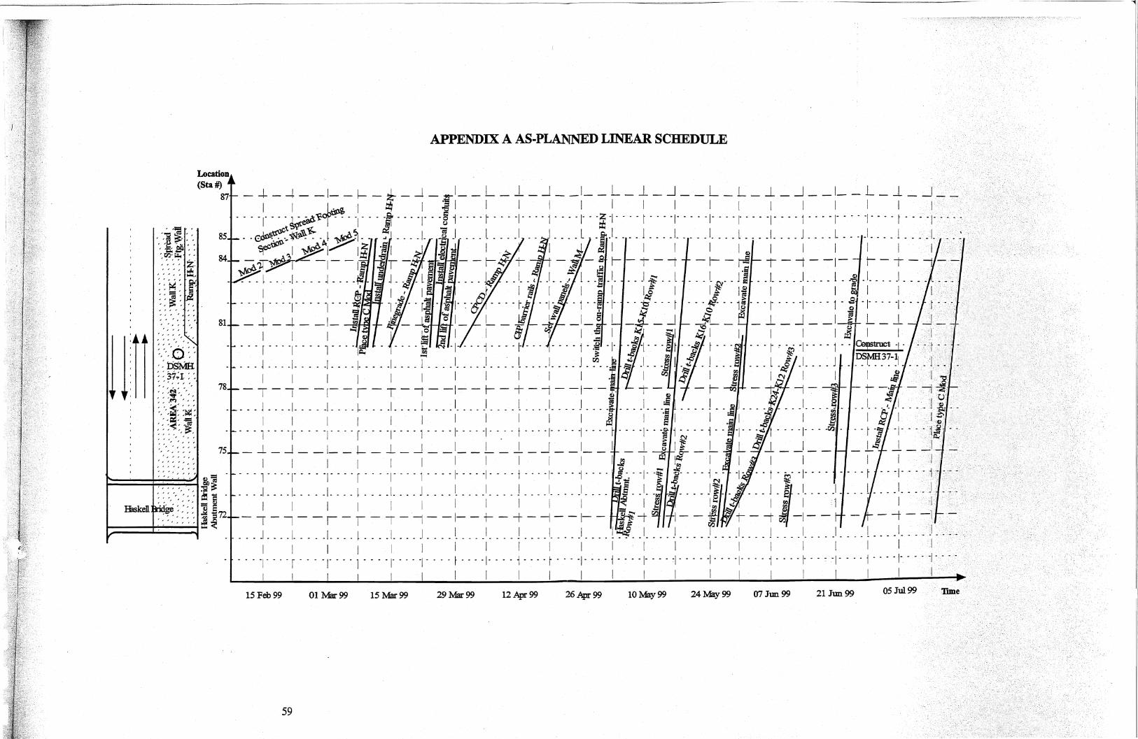
T
.--,"-:.:;
,\ (~,
I .1
:' ..
!.' I
. ," ".' I
'
I .
I
f::! JIlIM
. lOO
mln
qv
~iJP!-{IlI~J(lMI

LINEAR SCHEDULE (cont'd)
_ -t __ 1 __ ~ _ -+- _ -+ - -1- - 1- - +-- - + -:- -l - - 1- - L - J I 1 I 1 I 1 1 I 1 1 1 1 I ," ,_,"'"' .. _'. "' __ " _. _.- I - - - - -I " - - - - - - - - - - - - I" - - - -1- - - - r - - - -1- - - - -I - - - - - - - - . - . - - . - - . '1- . - - I l'f~H""":;'r. ., .. ,,' ,", I-p ,... 1 I I I I .. · .. · .. Jii{i : ' ":1 ... ' .........•...• ' ..... -.-: -f i ----:- ----I ----i ---: ----: ----: ----: ' ---~ , ---: -,- , i ----: ---:
.. "-+ !-=r~-. "-'- r - - r'J..-r/-I- -1- - - -, T -1- -1- -,-,-,- - 1- -1- 1 _ _ - " f - - . -1- .. - - . t - - - -1- - - ~ - - - . 1- - - - -I - . . - ~ . . . ' 1- - - - t - . . . 1- . . - ~ . - - - 1
I I I 1 I 1 I I I I I I I 1 T . -- i --- -I' . - - -I . - - . \- - - - r -.. r - - - r -- -i - - - ' 1' - - - i . ---I' .. - '1 . - - - r L _ + _ --1 - 1- - -w + - -+ - - 1- - 1- - t- - -+ - -1 - - 1- - .L
- ~ - - - -:- - - -: - - - - f - - -,,'" 1- \ ----: ----j --- : ---: ----f - - - -: - - - -: - - -: -I - - - - ~ - - - - - - - - r - -# --9 --1 - - - -1- - - - -\ - - - -I- - - - -I - - - - t - - - -1- - - - j - - - - I ~ _1-3 I __ I _~ Il_.L .- i _ J __ 1_- L _l_J - _ 1_- ~ I 1 .. 1 1 til@' I I I I I I I I I I 'fj ~ -~ __ f - - - -1- iI -1 - - - -1- - - - i.:t:-- - - - t - - - -1- e- - f - - - -I- - - . 1- - - -1- . - - -1- - - - \- - - - -I·
_ I _ _ _ _ I ~ _ J. _ _ _ I _ 1- _ _ _ I tl- _ I __ - .I. - --L - - -I. - J - - I - - _I I I I I I I #. I I I I I I / 1 I - 1- - - t- - -t - ---j - 1-'- - ~.f'+ - -+ - - 1- - r- - t- - -t -~I- i1 1-- -:-- - J - -: - - - -: - - - i -~ --j ---1- -: ;" ~ : --_ I_g - -1l 'd- : ~9~ II
- -~:~-, ~<t~-~-~~ ~ ~ A#~~fli~-:--: : :: : : .1 : : : : ; : : : ::: : : : r : : : :!: : ,Tf!!: : :o¥1 : : : : f ! -::: : : : r : : : r : : : 1·
I I I
11 Oct 99 25 Oct 99 08 Nov 99 22 Nov 99 06 Dec 99 20 Dec 99 'lime
60

APPENDIXB
SCHEDULE WITH PROPOSED CHANGE #1
~ \
-~ .. ,.
61

!!!!!!!!!!!!!!!!!!!"#$%!&'()!*)&+',)%!'-!$-.)-.$/-'++0!1+'-2!&'()!$-!.#)!/*$($-'+3!
44!5"6!7$1*'*0!8$($.$9'.$/-!")':!

/o.1t'.',.
P '.!'
'"
Location (Sta'lf)
84L._ .J _
" '0"" ,;' , " ,; " -,
':OsMH ',: 37;r:',
81
, ", " , 78 :: :~', " ' , ,,"!!" "
:, <~~: :~:, '" : '-=,='
'" ,,~ce , ,; .. '"
~ ,:,~,>': ': ':, 75 ,; ,~. " , " " "
' .. ' .. ',,',
,
25 Oct 99
63
/)0, ' / 1 \\ (J v
APPENDIX B SCHEDULE 'VITH PROPOSED CHANGE #1
08 Nov 99 22 Nov 99 06 Dec 99 20 Dec 99 TIme
Fragmented Planned Schedule
Location (Sta'lf)
81
78
75
, I , I I I I I _1_ -"- L _ ..l __ 1 __ L - 1- - -1 - -I-
I I I I I I I I I " ---T---'----r---T---'----r---T---l----r---T _ _ _ -' _ _ _ _ _ _ _ _1__ _ _ -' _ _ _ _ l _ _ _ _1_ _ _ _ -' _ _ _ _ l - - - -1- - - - -"-
, I I , , I , I I I -r-- ~-'--r-I-I--I-,--I-I--I-
- - - - i - -,- t- ---,- ----I - - - - r - - - -1- - ~ - -I - - - - r - - - -1- - - - -1-, ~ ~ . ' , , I I I I I
- - - t gj -~I- - - - -, - - - - t- - - -1- - - - -I - - - - t - - - -,- - - - -,- - - - t -_ ~~~ _ .J __ 1 __ L _.1 __ 1 __ , __ 1. _-.1_
!8 ~ I I J I I , , , I ·s ~ - - - t k -1- - - - -1- -It - - - -,- - - - -I - - - - t - - - -1- - - - -I - - - - t -
____ I J _ -' ----1 ~6 ~ __ 1 _____ , ___ - 1 - - - -,_ - - - _, - - - - j - - - - I-
I ~().~: I , , , 'r,$! 1 .... 1
--,- - t- ~ ~ -I - - r - -t- - ---t - - ~~ - t- -p -t ~~ I ... I i.- I I :t?( ~ - - - -/:
I ~f' ~ '~f!1 ~ 72~-~ ~ ~ -.:I4I;·'·I}!~Ja~~~''iI41f-~·~ 1 ¢J '4f , ~ 1 ru, I:... i ~ . , ~ 1
- - - -1- - - - 1 - -1- :'-l~ - -I ~ - - 1 - - - ~- - - - -I- - - - 1 - - -°1_ - - - "i-I I OJ~ I : I , ~, " I , ,
- - - - - - - - - 11- - - - - - - - - - - - - - - - - - - - - - - - - - - - - - - - - - - -I l..~ , : I I I I I I I
25 Oct 99 08 Nov 99 22 Nov 99 06 Dec 99 20 Dec 99 Time
Anticipated Schedule Impact
II
"

!!!!!!!!!!!!!!!!!!!"#$%!&'()!*)&+',)%!'-!$-.)-.$/-'++0!1+'-2!&'()!$-!.#)!/*$($-'+3!
44!5"6!7$1*'*0!8$($.$9'.$/-!")':!

APPENDIXC
SCHEDULE WITH PROPOSED CHANGE #2
n I I
• . J
u
' l
LJ
65

Ii .. ' i! ;
66
,:
L'
r'
"

, ',:: L,' ~ " " ,
" " ''-.:, .... .; ", ';"<
:,"':'0:," ': DSMff, : : 37~r : ~ , ...... "'" ,
{ ~"~;~~':: ",: : =
"~ ;',: " p;>-, "" "', .. , .. ", '",
" , " .. ", " , ", ''', ",
. , . . OI)~ ',,,, "0;;> " : " " " :: is ..... ~~::: ~~
84
81
78
7S
£j,:::":". ~= '",::', ~ ::s
: " " " " ~ .~ 72
Location (Sta #)
09 Aug 99
67
APPENDIX C SCHEDULE "TITH PROPOSED CHANGE #2
81
78
75
72
23 Aug 99 6 Sep 99 20 Sep99 04 Oct 99 'TIme
Fragmented Planned Schedule
Location (Sta #)
09 Aug 99 23 Aug 99 6 Sep 99 20 Sep 99
Anticipated Schedule Impact
l
lime 04 Oct 99
,--

!!!!!!!!!!!!!!!!!!!"#$%!&'()!*)&+',)%!'-!$-.)-.$/-'++0!1+'-2!&'()!$-!.#)!/*$($-'+3!
44!5"6!7$1*'*0!8$($.$9'.$/-!")':!
APPENDIXD
SCHEDULE WITH PROPOSED CHANGE #3
69

!!!!!!!!!!!!!!!!!!!"#$%!&'()!*)&+',)%!'-!$-.)-.$/-'++0!1+'-2!&'()!$-!.#)!/*$($-'+3!
44!5"6!7$1*'*0!8$($.$9'.$/-!")':!

(
APPENDIX D SCHEDULE WITH PROPOSED CHANGE #3
',:',',1: , '" ,I,
'''''~
'::'>~'::, " .. \",.,1'"
': t)sMR " ; 3:;;1 : "
(~ .J ,",~',;:a ' """i:f i .. "", .. , ..
.. .. " ..
Location (Sta #)
84
81
78
___ ~_ ~ __ L_l __ -_L_-, I , I I I I I I
- - - -I - - - - t - - - - ~ - - - -1- - - -, - - - - 1 - - - - t - - - - 1- - - - -1- - - - -
I I I I I I I , I - - - -I - - - - i - - - -r ---i -r -r ---r ---i - - - -1- - - - - ,- - - - -
~ . I _~_~ _~_ L~ __ ~_~_~ __ ~ __
I I S 6 I I I I I - - - 1 - - ~ - - - - -1- - -/1 ~- - - l - - - - 1 - - - - I" - - - -I" - - - -I - - - - -
___ j __ ~ I. ____ 1 __ ~ _~ - - - 1. - - - 1- - - -L - - - -1- - - - -1- - - - -
I .~ I I ~ of I I I I I -t-~ 1--1- ~-I--If-I-I--I---
----:i -:----: --l: ---i /'1- --:- --: ---i ----, , "" ",
, ' 00> " , , " ', ' ];;> ~' '''' ~=ca
-,---i ---:- ----: - --; ----if. ~ --~ ----. 1- - - - -: - - - - ; - - - - ,
75..L - -1- -I -r~- -1- -I:- -1<;~-I- --. - ~ - -~~- .
, 4~ ~ - ~\G ~~ i
, ' , " <,', ~-a " " "" = G)
~~~':'" ~.E '1<U6e '" ~ = , :', " , " 'gj..t;l
' "" ~~ 72 _ L _ -L _ ~ ~~ - L -:..L _ -}yJ1L~..L - -1- -.
----: ---: ----: ----: ---: -:- --/1- --i ----: ----~ ----1 1 1 :1&$' 1 1 I · '----.
11 Oct 99 25 Oct 99 08 Nov 99 22 Nov 99
Fragmented Planned Schedule
71
Location (Sta #)
84
81
78
, I I I I I "I - -I - - - - 1 - .;....1- - L
- - - , - - - - I - - - , - - - -1- - - - -I - - - - 1 1 1 1 --___ 1 ____ 1 1 1 1 ,----1----,----1----
I I - - -r --~ ----------J - - - - ! ----1- - I _ +- _ {:J. ~ I I I I I - - -,- - - - -__ ~ I I
1 4 !; +---;--f---'+-~--f- -- - - - - - ~I ~ I I I I - -1 r --i I -§- - T - - - l - - - - - - - - - - - - -1- - - - I ___ 1 :S L r, ge . I I , -I - - - - -
_ !Ii _ _ _ _ ~.11: I J I ~ ~ - f - ------ ----1 - - - - 1- - - - ~ 1-_ ,-i 1 ~ l'tl 1 1 1 ' - .. I .. -TOt -j- ~-t---j ___ I 1 1
..ll, .. I.. 11 1 ? 1 t- - -j - - 1- - -? I II - - - - -I - - -j.~- - - - 1- - - - -1- - - - -'- - - - J. - - - ,
- - - - r. - - - -1- - - -1- - - - -I - #.._ I I II v.,q, f - - - -i ----1- - I 75..L.... _1_ I .1 ~ I - - - - - - - i - - - - .
__ I I I -~~~ C? - -I - ~- - - ~ J - _1-__ • I OJ ~~G..';; I - -.... _ i .. &.~ -- _:1" .. -I- .. _ 0 .. .-
__ • __ 1 _____ I,(~' 't'. :1 1 ~t e,"~Q -r-r So- - -1- - - -I 1~ I, ----, ---------'S I ~-vf - _1 - b~/ I
72.l.- I ~t-I '".,,~ ,I I If . A I - - - - - - - - -___ -l- Y -J 'L l}j 0"', I
_ _ _, - -l- 4P', 1- ~ L .... I.. 1 1 :1 1 Iii"'; <; - -L - --1- -
I ---I---- l ----:r----~ ':-'- ----1--- I I . " ,c1/ff I I - I - - - - I" - - - -I
11 Oct 99 25 Oct 99 08 Nov 99 22 Nov 99 1ime
Anticipated Schedule Impact
--.~----.--- -- i
r

!!!!!!!!!!!!!!!!!!!"#$%!&'()!*)&+',)%!'-!$-.)-.$/-'++0!1+'-2!&'()!$-!.#)!/*$($-'+3!
44!5"6!7$1*'*0!8$($.$9'.$/-!")':!

APPENDIXE
SCHEDULE WITH PROPOSED CHANGE #8
73

!!!!!!!!!!!!!!!!!!!"#$%!&'()!*)&+',)%!'-!$-.)-.$/-'++0!1+'-2!&'()!$-!.#)!/*$($-'+3!
44!5"6!7$1*'*0!8$($.$9'.$/-!")':!

(
APPENDIX E SCHEDULE WITH PROPOSED CHANGE #8
Location ,,= ' (Sta #) '~~ " " "e ' .. ~', " 1 1 1 1 1 1 1 1 1 '~~ " >':~~: 84 I __ L_~_~ __ I~_.L_J __ I __ I-,',:::::t, 1 1 1 1 1 1 1 I ' 1 1 ':j(.~ ···l····r···T···l····I····T···l····r···T··T· ":a'A : ;~', " ., .l ... 1 .... J .... l .... 1 .... .1 .... l .... 1 .... .1 ... .1 .. ', :',',,',: 1 1 1 1 1 1 1 1 1 1 :':'~~':,,:'-": 81 -I w r- - -r - - 1- -1- - I - I - -1- - r- - r-" : :, ", : : , .... t . i .. 1 .... J .... I. .... 1. : .. J .... I. . ; .. 1 .... j ... J . :':',9,-,' ~ G I I I I I 1 1 1 1 : " P~ . . ·1Ji . ~. . 1 . . . . r . . . '1' . . . 1 . . . . r . . . ' 1' . . . 1 . . . . r . . . r . ,,37,.1, , ~ 0
: : ; : : " " C,) I. ~ I 1 I I 1 I . 1 I I ,~, 78 ¢iJy§--------------------: : :,~:-; > ~ ~ . 1 I I I 1 I I I I \ ~ ~~ :;: ., ~... i . . . '/~~ . .:. . . . : . . . . :. . . . .:. . . . i . . . . :. . . . :. , ~, . i········ ~ . . . . . . . . . . . . . . . . . . . . . . . . . . . . . . . . . ",<> >, I I ~/I I I I I I I I 1 """', 75-1- - ~1J.Jf/--t - - 1- - r - -j- - -j - -1- ~ t--8
I====t:::;:': ~=: : =~ ~:::;:':':~.. i i ... i~l: . i .. : ~.d· . i i . -l.l'i(:: }:. Hasken~~'~'<: ;! . ~~~. -- .. : .... i .. '.J~~~~#~' j . k~·. "§W~~rtJjiAC1:flJ· tf'; .
" " " , " :l@ ";J 72 ~ - - - - - ---1tW ~ . JJ ~ -~ -bt:! - -
I;::=::::l='::' =' '=' ::j" ::t ~ :# I I I'~ cY. I t::; ~ I.e' 1 , ~ .:f. I' ... '1' ... jl~ ~I'" ~'I' ... j ./ .. I~~ .. ~I' ... e-- . j .
... .I. __ . J . . . q;~ __ •• 1 .... J. . . . I. ~. . .I. __ . J . . .. I ...• I .. 1 I S;1i I 1 I I I I 1
25 Oct 99 08 Nov 99 22 Nov 99 06 Dec 99 20 Dec 99 Time
Fragmented Planned Schedule
75
Location (Sta #)
I I 1 1 I 1 1 I
84-l- _ 1.. _ --1 _1 __ L _ J. __ I _ - L - 1.. - -1 - -I-I I 1 I II I I I I
. . . T . .. .., .. r . . . T . . . 1 . . . . r . . . T . . . 1 . . . . r .. . T
... .1 ........ 1 .... .1 .... l .... 1 .... .1 ..... l .... 1 .... .1. I I I I I I I I I I
81.1_ - I - ~ - 1- - r- - I - -r - -1- - r- - -r - -I -~ is .... ·1 .. i. . j -- . ·1· ." . ·1 .... r . . . '1' ... l .... r ... ·1' ... '1 .
I ~ n i l 1 I I I I 1 . . . t ~ . ~ I' . . . '1' . . . t . . . . I' . . . '1 . . . . t . . .. I' . . . '1 . . . . t .
78L. _ Ii ~l. _ .J __ 1 __ L _ J. __ I __ 1 __ .1. _ -.l . ~ .t I I J I I 1 I I I
. . . t k' I' . . . '1 . . . it· . . . I' . . . '1 . . . . t . . . . I' . . . '1 . . . . t . I ~ I I -.II I I I I I I . ... ~ ....... :!I.6 .... ···················•··•····
1 m I· I I I 1 II I I 75..L. -/1- - t- - --.; - 1- - .t- - T - -i - -J'S - t- -8-t
. -I: --. ill- -f .: -. i, ~ . . -1 -. ·c :. . ;.,OJ 1#_,) l-: n~)I_~~61W~:·7vil~t!I~~~+
.. - ·1 - .. - i . I .: --1'< .. i .. -~ . - - -I- - - . i .. -t ... -I-I I O;~ I : I I &61 I I I 1 . ........ f· .......... . ......... , ............. . I ~ 1 : I I I 1 I I I
25 Oct 99 08 Nov 99 22 Nov 99 06 Dec 99 20 Dec 99 TIme
Anticipated Schedule Impact ,-

!!!!!!!!!!!!!!!!!!!"#$%!&'()!*)&+',)%!'-!$-.)-.$/-'++0!1+'-2!&'()!$-!.#)!/*$($-'+3!
44!5"6!7$1*'*0!8$($.$9'.$/-!")':!

APPENDIXF
PROPOSED LINEAR SCHEDULE FOR REVIEW
77

!!!!!!!!!!!!!!!!!!!"#$%!&'()!*)&+',)%!'-!$-.)-.$/-'++0!1+'-2!&'()!$-!.#)!/*$($-'+3!
44!5"6!7$1*'*0!8$($.$9'.$/-!")':!

UUA\ t IJa1ll1 nqy
a8p!-lI na)fSllJI ,
, '
" J
-',',
' I
I()
......
...... o

,.1 '_
.
ltuA\ llJaU
Qn
qy
Qiip!-lI lI Q::>fS13fl
~ ,
, ,
' ',,,, ',',',
' , ~'
, ,
')lWM
'
, "
, ,
"',
' ,
'''-fiI ~ '\
' , ' , '/ '0"
~',',' , , ' , ' , ' , ' , " ','.', ',',
' ,
"...., ""
.'
" "
, ,
, ,
" ""
'~M .... ,j: .. : : : :1tU~M: .<:. : : . ~ :;; : ,,;".£'vmIv.. .. :. : : : : ... l .
. ~~:< >: <
><.::............ .. .. ..
. ... ~ .. I ....
:i! -~ -
--
--
--~-
--
--
-
~.
o 00

APPENDIXG
SCHEDULE COMPRESSION QUESTIONNAIRE
81

fIIII'1 {d
r
1, Ij
I:
I . ,
I
•• I
• I
-II
II
II
II
nl i
II~
II~
IIli
1111
1:111
IIH
1111
nn IIH -L:
--- -------~,-
APPENDIXG
SCHEDULE COMPRESSION QUESTIONNAIRE
Please respond to the following questions by choosing the most appropriate answer .
Provide brief explanations pertaining to your answer.
The questionnaire is filled out by:
J.dyleJ;13rl\.-,J~r'pj~~.tEJl.,gi.I!~~rl..oJ:..GrilJljj~J;Jm§tt1J~!icp'LC_Q.1ll..R3!1.Y ..
Utilized Technique: Overlapping
1) Subject Activities: Constructing planter terraces and constructing planter windows.
Suggestion: Overlapping the activities by allocating an additional crew.
Response:
a) Can not be applied
b) Will be applied
c) Already applied
The limiting factor is the additional crew, which we do not have at this time. However, in
the future we feel that we can have two crews devoted to these activities upon the
completion of the waterproofing,_ etc.
2) Subject activities: Continuous reinforced concrete pavement (CRCP) and constructing
cast-in-place barrier rails.
,-
Suggestion: Starting the construction of the barrier rails two weeks after the paving starts r' as opposed to a finish-to-start type of relationship.
Response:
a) Can not be applied
b) Will be applied
c) Already applied
82

We have the barrier crew starting after the outside shoulder and
shoulder is poured/cured. This is the minimum room required as
suggestion.
3) Subject activities: Constructing the barrier rails and installing pre-cast wall panels.
Suggestion: Overlapping the two activities with 6 days of lag between them.
Response:
a) Can not be applied
b) Will be applied
c) Already applied
We have the panel crew starting approximately 5 days after the barrier rail crew. By this
time the barrier rail crew proceeds forward. In that way, enough working space is
provided for the panel crew.
Utilized Technique: Increasing Utilities
4) Subject activity: Installing underdrain between Sta. 71 and Sta. 85.
Suggestion: Allocating an additional trencher and a backhoe with supporting crew.
Response:
a) Can not be applied
b) Will be applied
c) Already applied
After analyzing the situation, we decided that a small quantity of remaining underdrain
does not warrant hiring a second crew and acquiring equipment.
5) Subject Activity: Constructing cast-in-place barrier rails.
Suggestion: Allocating another crew and a crane.
Response:
a) Can not be applied
b) Will be applied
83

J, ;;
" ! r ~<
I"',',. ,
I', , '
I,'
Ii; ,I, (II
!t l ld ,
H' ~'
Iii' :11 I,
Iii ,il
~1 Ii: 111, HI
c) Already applied
At this point in the job, with a small quantity of barrier rail remaining and overall
schedule showing that barrier rail crew is staying ahead of the panels but is not catching
up with the paving crew, we do not foresee the application of the suggestion.
6) Subject activity: Setting pre-cast wall panels
Suggestion: Allocating another crew just for the panel closures.
Response:
a) Can not be applied
b) Will be applied
c) Already applied
Second crew is pouring the closures and the suggestion has worked well.
Utilized Technique: Changing the technology used.
7) Subject activity: Continuous reinforced concrete paving (CRCP)
8)
Suggestion: Using 'class K' type of concrete as opposed to 'class A' type of concrete.
Response:
a) Can not be applied
b) Will be applied
c) Already applied
The use of early strength CRCP is to be determined by TxDOT. Extra cost associated
with this would fall to TxDOT taxpayers. However, this is a very important idea to
accelerate very specific pours.
Subject activities: Drilling tiebacks, stressing tiebacks and excavating for the next row of
tiebacks.
Suggestion: Starting excavation right after drilling the tiebacks. Man lifts will be used to
stress the tiebacks after excavation.
Response:
84

a) Can not be applied
b) Will be applied
c) Already applied
This has been applied at our last wall, Wall H, and worked very effectively. The
drawback to this is in the case of Wall H; we had a minor failure in top row, which
caused us to rebuild a bench to allow the tieback to be redrilled.
The application may not be cost effective if more failures are encountered.
85

!!!!!!!!!!!!!!!!!!!"#$%!&'()!*)&+',)%!'-!$-.)-.$/-'++0!1+'-2!&'()!$-!.#)!/*$($-'+3!
44!5"6!7$1*'*0!8$($.$9'.$/-!")':!

APPENDIXH
,- , LINEAR SCHEDULE WITH APPROVED CHANGES
I I
__ J
87

!!!!!!!!!!!!!!!!!!!"#$%!&'()!*)&+',)%!'-!$-.)-.$/-'++0!1+'-2!&'()!$-!.#)!/*$($-'+3!
44!5"6!7$1*'*0!8$($.$9'.$/-!")':!

unM luauqnqy
3ilPl-ll ll3)[SIlfI
/' ~'
, ,
')1 JlUM
' , ' , ' , ' " , " , ' , '
"'N~~",,,',"
'0' ',"
, """"
, """
p"
'.-t,
, ,
, ,
I~"':""': : ' : " ... ~.< : : : : " flli;' ,it. WRY •• : : ' > > . , • " : :!> :
pll.~lJdS '"
, '
, '"
, ",
,'"""
, ' , , ' ,> ~:: ,' .. ', -:, :-,',< -: ' ... :' ... , ' , :-, ' , ' , ' , ' , "
""~' , '
, ,
, ,
, 1
] ,
, ,
, ,.\4
.... ~
-------
-----
.. ..
o .... .... o

Location (Sta #)
" , "9 (II
" 'u ~,' , " IS: ~, '
, ,tZl,f;:I.", , , ',:',', '>7
, ,'" ~ , '" '' j...I.f ,:',' , " ' Q " ,' , ~' ,13 :- :- :- ~ , ~
.. ' J~ . '
, , , ,:" ,
(
APPENDIX H LINEAR SCHEDULE; WITH APPROVED CHANGES (cont'd)
I I I I I I I - T - -1- - "I - I" - -1- - T - -1- - "I - I - -1- - T - -1- - "I - I - - 1- - T - -1- - . . . . . . I· .. . .1.. . . . ·1- . . . -1 . . . . -1 . . . . ~ . .. . 1 . . . . t . .. . J . . . . ~ . . . . I· . . . . I· . . . -1- . . . -1- . . . -1 . . . . ·1 . . . . -1 . . . . .
8SL I I · I I I I I I I I I I I I I I I ..... I' ... -1- ... '1-· ·-1 ···-1-···-1 ... I· ... 1 .... f .... r .... r .... r .... I' ... '1- ... -1- ... -1- ... -1-· ...
I ~ __ L __ I _&1 L _ J. __ 1 __ 1- _ ~ _ - L - .1 - _ 1- - L - ~ - - . I I I I 8. s 1 1 I · I 1 I 1 1 I 1 1
··~·I ···-1-···1 ·-05 .... j ... -5 ·-05 I·· ·1-····I·····I·····I·····I·····I···· i ····i····j····j·· ... .~ I I. ';' 1 C:- I ~ 1 1 I 1 1 1 1 1 I 1 1 . ···-1-···· '., C!) '1 . . .. '·.1 i . .. (L) • i .. . i . . . . I· . . . . I· . . . . I· . . . . I· . . . '1- . . . -1 . . . . -1 . . . . -1 . . . . -1 . . . . .
87
84
81 -1- -' -i - I-;f -+- J-I- +- - --+ -- - 1- - -+- - -I - - +- - --+ - - 1- - + - -1- - -
--··1-/- -.: ---. -~ -: -. . -~ -~ ~ -~ - j if -ID ----: -' --. : . ---:--. - :. -. . .: --. -: --. --: -----: --. --: ---. -. . .• ~ .... I. . . . . . . , . .I. . . . .I . . . . .I . . . . J ~ . ~ J . . . . 1 ... . . l . . ... L . . . . L . . . . I. . . . .1. . . . .I. . . . .I. . . . J. . . . .
:+ .[ »<:: "\ :,', " '0' " . , . , , -
~- = ~ _ .... 5 ~ I I 1 1$ ~ I ' 1 I 1 I I I I I 1 , " ,N , , - -a ~ -i - - ~ f- + - - ,l t- - --t -.;. - f- - + - - 1- - +- - -t - - 1""- - -r - -1- - -
, ' ,~: ' : ' ' ~ CIS .!I 3 I ~j Is 1 ts] 1 I 1 I I . I I · I I 1 : 1 ~ -~ -:! : ~ 1- -.; 1 'I;--~ .@. - I - - - 'F-~ T -- T/i - -- r - . r ---1- - - . F - Y -- -Y -- -I - -, ' , ' " '::> . := . l.rQ . i 1 ..~. I. . 6- I . ..s...~ ...1-···-1 .~. ~ . . . . j .1 .. ~ . . 1 . . . . l . . . . L . . . . L . . . .1- . . . .1. . . - -1- - . . -1- . . . .
" , ? c.... li"') I .= ~'
, ' , -', -: .-, 7S ~ f.o &. -: T - I . - --r - -I - T -;, ~ - I - --r - - 1- - "I - :1 - - ,- - I - -1- - -
, ' ,'.D~MH . ' , . . 37..,1 , .
78 .. y .
<,' , , .! 0 ~ I I ~. I I ~ 1 ff.N 1 I lit I I I
: : :: 1'0 ~ - il ~ - IJ :- -t :---: 1-~ -- -: ----- --kO: -: t --j ~ ~l-- --:- -g- -:. :,./ [-l ~ --: ----: ---HoskoDl4:: :: ;;72 ~ _ :~5: __ J5~1 -~-l-~-~-I-~~ ) ~ JI«~-· tI.%·l;AI;~4 '1J!!ljj~~~I~' ~ 1 ~ ~:~ ~ ~
,' , ' , , , .~.Q 1 I I ~~~ I I .~' I~ A~ -!/~ It!flWJ1 I I 1 1 ::t <l:; iJ'~ ~ ~ !~ C}"· IS ~o & r:-t r-., 1
- - • - : - - - - : - - • - :- - - - -:. - - -: - - - • -:. • <0 '1'# -- -: l:l-1- --~ --I : --I : ----:-b- - i:-- -: - ---:- ----... - 1 . - . - r .... r .... I' ... -1- ... -1- ... -1- ... -1- . ~f·l· i - . 1 - - - . 1 .... t .... t .... r .. . t I· . - . - I· .... I· ....
· 1 I I I I I I I f I i I I I I 1 II I 1 .. 37 3S Tune 2S
02 Aug 99 27
16 Aug 99
29 31 i D ~Aug99 D~~ ~~99 11 Oct 99 2S Oct 99
90
!h i
l ,, -., . ~. , (
I
II
I I