ScatteringandDecayofParticles - Freie...
63
All human things are subject to decay, and when fate summons, monarchs must obey. John Dryden (1631-1700) 9 Scattering and Decay of Particles So far we have discussed only free particles. If we want to detect the presence and detailed properties of any of them, it is necessary to perform scattering experiments or to observe their decay products. In this chapter, we shall develop an appropriate quantum mechanical description of such processes. 9.1 Quantum-Mechanical Description We begin by developing the appropriate quantum-mechanical tools for describing the scattering process. 9.1.1 Schr¨ odinger Picture Consider a quantum mechanical system whose Schr¨ odinger equation ˆ H |ψ S (t)〉 = i∂ t |ψ S (t)〉 (9.1) cannot be solved analytically (here we use natural units with ¯ h=1). The standard method of deriving information on such a system comes from perturbation the- ory: The Hamilton operator is separated into a time-independent part ˆ H 0 , whose Schr¨ odinger equation ˆ H 0 |ψ S (t)〉 = i∂ t |ψ S (t)〉 (9.2) is solvable, plus a remainder ˆ V , to be called interaction. The operator ˆ H 0 is also called the unperturbed Hamiltonian, and the interaction ˆ V is often called the per- turbation . For the sake of a simple notation we have omitted the hats on top of all operators without danger of confusion. The time-dependent state |ψ S (t)〉 carries a subscript S to indicate the fact that we are dealing with the Schr¨ odinger picture. Observables are operators ˆ O S (p, x,t) whose matrix elements between states yield transition amplitudes. The interaction will be assumed to be of finite range. This excludes, for the moment, the most important interaction potential, the Coulomb 660
Transcript of ScatteringandDecayofParticles - Freie...

All human things are subject to decay,
and when fate summons, monarchs must obey.
John Dryden (1631-1700)
9
Scattering and Decay of Particles
So far we have discussed only free particles. If we want to detect the presence anddetailed properties of any of them, it is necessary to perform scattering experimentsor to observe their decay products. In this chapter, we shall develop an appropriatequantum mechanical description of such processes.
9.1 Quantum-Mechanical Description
We begin by developing the appropriate quantum-mechanical tools for describingthe scattering process.
9.1.1 Schrodinger Picture
Consider a quantum mechanical system whose Schrodinger equation
H|ψS(t)〉 = i∂t|ψS(t)〉 (9.1)
cannot be solved analytically (here we use natural units with h=1). The standardmethod of deriving information on such a system comes from perturbation the-ory: The Hamilton operator is separated into a time-independent part H0, whoseSchrodinger equation
H0|ψS(t)〉 = i∂t|ψS(t)〉 (9.2)
is solvable, plus a remainder V , to be called interaction. The operator H0 is alsocalled the unperturbed Hamiltonian, and the interaction V is often called the per-
turbation. For the sake of a simple notation we have omitted the hats on top of alloperators without danger of confusion. The time-dependent state |ψS(t)〉 carries asubscript S to indicate the fact that we are dealing with the Schrodinger picture.Observables are operators OS (p,x, t) whose matrix elements between states yieldtransition amplitudes. The interaction will be assumed to be of finite range. Thisexcludes, for the moment, the most important interaction potential, the Coulomb
660
9.1 Quantum-Mechanical Description 661
potential. As an example, we may assume the unperturbed Hamiltonian to describea particle in a Rosen-Morse potential well:
〈x|V |x〉 = V (x) =const
cosh2 |x| . (9.3)
If the constant is sufficiently negative, the system has one or more discrete boundstates. The important Coulomb potential does not fall directly into the class ofpotentials under consideration. It must first be modified by multiplying it with avery small exponential screening factor. The consequences of an infinite range thatwould be present in the absence of screening will have to be discussed separately.The interaction V may in general depend explicitly on time.
The results will later be applied to quantum field theory. Then H0 will be a sumof the second-quantized Hamilton operator of all particles involved, and V will besome as yet unspecified short-range interaction between them. If the particles areall massive, all forces are of short range. Moreover, the vacuum state is a discretestate which is well separated from all other states by an energy gap. The lowestexcited state contains a single particle with the smallest mass at rest. This mass isthe energy gap.
9.1.2 Heisenberg Picture
The other, equivalent, description of the system is due to Heisenberg. It is basedon time-independent states which are equal to the Schrodinger states |ψS(t)〉 at acertain fixed time t = t0:
|ψH〉 ≡ |ψS(0)〉 = U(t, t0)−1|ψS(t)〉. (9.4)
For simplicity, we choose t0 = 0. When using these states, the time dependence ofthe system is carried by time-dependent Heisenberg operators
OH(t) = U(t, 0)−1OSU(t, 0). (9.5)
Here U(t, 0) is the unitary time evolution operator introduced in Section 1.6 whichgoverns the motion of the Schrodinger state. It has the explicit form [recall (1.269)]
U(t, 0) = T(
e−i∫ t
0dt′ H(t′)
)
. (9.6)
If H has no explicit time dependence, which we shall assume from now on, thenU(t, 0) has the explicit form U(t, 0) = e−iHt/h and satisfies the unitarity relations
U−1(t, 0) = U †(t, 0) = U(0, t). (9.7)
Then the relation (9.5) becomes
OH(t) = eiHt/hOSe−iHt/h. (9.8)
662 9 Scattering and Decay of Particles
9.1.3 Interaction Picture
As far as perturbation theory is concerned it is useful to introduce yet a thirddescription called the Dirac or interaction picture. Its states are related to theprevious ones by
|ψI(t)〉 = eiH0t|ψS(t)〉 = eiH0tU(t, 0)|ψH〉. (9.9)
In the absence of interactions, they become time independent and coincide with theHeisenberg states (9.4). The interactions, however, drive ψI(t) away from ψH(t).
When using such states, the observables in the interaction picture are
OI(t) = eiH0tOSe−iH0t = eiH0te−iHtOHe
iHte−iH0t. (9.10)
These operators coincide, of course, with those of the Heisenberg picture in the ab-sence of interactions. By definition, the unperturbed Schrodinger equation H0|ψ(t)〉can be solved explicitly implying that the time dependence of the operators OI(t),
d
dtOI(t) = [H0, OI(t)], (9.11)
is completely known. If the Schrodinger operator OS is explicitly time-dependent,this becomes
d
dtOI(t) = [H0, OI(t)] + [
˙OS(t)]I , (9.12)
where
[˙OS(t)]I ≡ eiH0t ˙OS(t)e
−iH0t. (9.13)
9.1.4 Neumann-Liouville Expansion
A state vector in the interaction picture moves according to the following equationof motion:
i∂t|ψI(t)〉 = i∂teiH0t|ψS(t)〉
= −H0|ψI(t)〉+ eiH0tHe−iH0t|ψI(t)〉= VI(t)|ψI(t)〉, (9.14)
where
VI(t) ≡ eiH0tVSe−iH0t (9.15)
is the interaction picture of the potential VS. It is useful to introduce a unitary timeevolution operator also for the interaction picture. It determines the evolution ofthe states by
|ψI(t)〉 = UI(t, t0)|ψI(t0)〉. (9.16)

9.1 Quantum-Mechanical Description 663
Obviously, UI(t, t0) satisfies the same composition law as the previously introducedtime translation operator U(t, t0) in the Schrodinger picture:
UI(t, t0) = UI(t, t′)UI(t
′, t0). (9.17)
Using the differential equation (9.14) for the states we see that the operatorUI(t, t0) satisfies the equation of motion
i∂tUI(t, t0) = VI(t)UI(t, t0). (9.18)
The equation of motion (9.18) can be integrated, resulting in the Neumann-
Liouville expansion [recall (1.200), (1.201)]:
UI(t, t0) = 1− i∫ t
t0dt1VI(t1) +
(−i)22!
T∫ t
t0dt1dt2VI(t1)VI(t2) + . . .
≡ T exp[
−i∫ t
t0dt′ VI(t
′)]
. (9.19)
The expansion holds for t > t0 and respects the initial condition UI(t0, t0) = 1.Note that the differential equation (9.18) for UI(t, t0) implies that UI(t, t0) sat-
isfies an integral equation:
UI(t, t0) = 1− i∫ t
t0dt′VI(t
′)UI(t′, t0). (9.20)
Indeed, we may solve this equation by iteration, starting with UI(t′, t0) = 1 which
yields the lowest approximation:
UI(t, t0) = 1− i∫ t
t0dt1VI(t1). (9.21)
Reinserting this into (9.2), we obtain the second approximation
UI(t, t0) = 1− i∫ t
t0dt1VI(t1) +
(−i)22!
T∫ t
t0dt1dt2VI(t1)VI(t2). (9.22)
Continuing this iteration we recover the full Neumann-Liouville expansion (9.19).For t < t0, we may use the relation (9.7) according to which U(t, t0) is simply the
inverse U−1(t0, t), and an expansion is again applicable. The time-ordering operatorT makes sure that the operators VI(ti) in the expansion appear in chronologicalorder, with all later VI(ti) standing to the left of earlier ones.
If V and therefore H has no explicit time dependence, the Schrodinger state isgoverned by the simple exponential time evolution operator:
|ψS(t)〉 = U(t, t0)|ψS(t0)〉 = e−iH(t−t0)|ψS(t0)〉. (9.23)
Combining this with (9.9), we see that
UI(t, t0) = eiH0te−iH(t−t0)e−iH0t0 . (9.24)

664 9 Scattering and Decay of Particles
If the potential V depends explicitly on time, this has to be replaced by [recall (9.6)]
UI(t, t0) = eiH0tT(
e−i∫ t
t0dt′ H(t′)
)
e−iH0t0
= eiH0tU(t, t0)e−iH0t0 . (9.25)
For a time-independent H , this relation shows that UI(t, t0) satisfies the same uni-tarity relations (9.7) as U(t, t0):
U−1I (t, 0) = U †
I (t, 0) = UI(0, t). (9.26)
The Heisenberg representation (9.5) of an arbitrary operator is obtained fromthe interaction representation (9.10) via
OH(t) = U−1(t, 0)e−iH0tOI(t)eiH0tU(t, 0)
= U−1I (t, 0)OI(t)UI(t, 0). (9.27)
We have observed above that the operator in the interaction picture OI(t) has aparticularly simple time dependence. Its movement is determined by the unper-turbed equation of motion (9.11). Thus (9.27) establishes a relation between thecomplicated time dependence of the Heisenberg operator OH(t) in the presence ofinteraction and the simple time dependence of OI(t) which reduces to the Heisenbergoperator in the absence of an interaction.
9.1.5 Møller Operators
Consider now a scattering process in which two initial particles approach each otherfrom a large distance outside the range of their interactions. This implies that at avery early time t → −∞, their states obey the unperturbed Schrodinger equation,i.e., that their wave function ψI(t) is time-independent. The same thing will be truea very long time after the scattering has taken place. Let us study the behavior of theoperator UI(t, t0) in the two limits of large positive and negative time arguments.In order to make all expressions well defined mathematically it is convenient tointroduce a simple modification of the potential by multiplying it with a switchingfactor e−η|t|:
V → e−η|t|V ≡ V η(t), VI(t) → e−η|t|VI(t) ≡ V ηI (t), (9.28)
with an infinitesimal parameter η. As far as physical observations are concerned,such a factor must have little relevance since η can be chosen so that V remainsunchanged over any finite interval of time. However, an immediate consequenceof the prescription (9.28) is that for t → ±∞, the state vector in the interactionpicture becomes time-independent, due to (9.14): Let us denote the limiting statesby |ψ in
out〉, i.e.,
|ψI(t)〉 →t→∓∞
|ψ inout〉. (9.29)

9.1 Quantum-Mechanical Description 665
Using the time evolution operator, the limit (9.29) may be written as
UI(t, 0)|ψI(0)〉 →t→∓∞
|ψ inout〉, (9.30)
i.e., the operator UI becomes a constant in the limit t→ ∓∞. Inverting this relationwe may write
|ψI(0)〉 = UI(0,∓∞)|ψ inout〉 ≡ Ω(±)|ψ in
out〉. (9.31)
The operators
Ω(±) ≡ UI(0,∓∞) (9.32)
were first studied extensively by Møller1 and are named after him. Their mostimportant property is the following:
HΩ(±) = Ω(±)H0, Ω(±)†H = H0Ω(±)†. (9.33)
To derive this, we consider, for simplicity, only the most common situation that Vhas no explicit time dependence except for the very slow switching factor (9.28).Then we multiply the explicit representation (9.24) of the time-evolution operator
by a factor e−itH and find
e−itH U(0, ta) = e−itHeitaHe−itaH0 = e−i(t−ta)He−i(ta−t)H0e−itH0 = U(0, ta − t)e−itH0 .(9.34)
In the limit ta → ±∞, this yields
e−itHU(0,∓∞) = U(0,∓∞)e−itH0 . (9.35)
The time derivative of this at t = 0 yields precisely the first equation in (9.33). Thesecond follows by Hermitian conjugation.
Let |ψ inout〉 be a steady-state solution of the time-independent unperturbed
Schrodinger equation:
H0|ψ inout〉 = E|ψ in
out〉. (9.36)
Then due to (9.33) [or directly (9.35)], the interacting state |ψI(0)〉 solves the fullSchrodinger equation with the same energy :
H|ψI(0)〉 = E|ψI(0)〉. (9.37)
In the laboratory, one does not really observe steady states but wave packets, whichcan be obtained from superpositions of steady-state solutions with different mo-menta. The packets of free particles approach each other and enter into the range
1C. Møller, Kgl. Danske Vidensk. Selsk. Mat.Fys. Medd 23, No. 1, (1945).

666 9 Scattering and Decay of Particles
of the interaction potential. Also there, the total energy remains the same, due toenergy conservation.
The amplitude for the scattering process is found as follows. Let |ain〉 be acomplete set of incoming eigenstates of the unperturbed Schrodinger equation
H0|ain〉 = Ea|ain〉, (9.38)
where a denotes the collection of all quantum numbers of these states. By applyingthe interaction operator UI(t,−∞) to the states |ain〉, these are transformed intothe time-dependent |aI(t)〉. After a long time, these develop into time-independentstates |aout〉. The energies Ea remain, of course, unchanged.
Let us analyze the outgoing states
|aout〉 = UI (∞,−∞) |ain〉 (9.39)
with respect to the incoming waves |bin〉. The scalar products 〈bin|aout〉 are obviouslyequal to the matrix elements of UI (∞,−∞):
〈bin|aout〉 = 〈bin|UI (∞,−∞) |ain〉. (9.40)
The right-hand side is defined as the scattering matrix or S-matrix:
Sba = 〈bin|UI (∞,−∞) |ain〉. (9.41)
The same name is also often used sloppily for the scattering operator
S ≡ UI (∞,−∞) (9.42)
itself, which can be written as a product of the two Møller operators (9.32):
S = Ω(−)†Ω(+). (9.43)
Since UI(t, t0) is a unitary operator, the S-matrix is also unitary and satisfies
SS† = S†S = 1. (9.44)
The Møller operators, however, are not unitary. As we shall see in the next section,the operators Ω(±)† are inverse to Ω(±) if H0 has no bound states. Under multiplica-tion of the states from the left-hand side one has
Ω(±)†Ω(±) = 1. (9.45)
In contrast, under multiplication from the right-hand side, the product yields aprojection operator onto the subspace of continuous states of the Hamiltonian H :
Ω(±)Ω(±)† = Pcontinuum. (9.46)
Note that only in an infinite-dimensional Hilbert space can it happen that the left-inverse is not equal to the right-inverse.
9.1 Quantum-Mechanical Description 667
9.1.6 Lippmann-Schwinger Equation
The solution (9.31) of Eq. (9.37) can usually not be given analytically but only inform of a perturbation series. This is found by inserting the Neumann-Liouvilleexpansion (9.19) into Eq. (9.31):
|ψI(0)〉= |ψin〉−i∫ 0
−∞dt′VI(t
′)|ψin〉+(−i)2∫ 0
−∞dt′∫ t
−∞dt′′VI(t
′)VI(t′′)|ψin〉+ . . . .
(9.47)
With the help of (9.15), and the damping factor as in Eq. (9.28), we see that thesecond term is equal to
−i∫ 0
−∞dteηteiH0tV e−iH0t|ψin〉. (9.48)
By assumption, |ψin〉 is an eigenstate of H0 with energy E, and V is independent oftime. Thus we can perform the integration and obtain
−i∫ 0
−∞dteηtei(H0−E)tV |ψin〉 =
1
E − H0 + iηV |ψin〉. (9.49)
Treating the other expansion terms in (9.47) likewise, we arrive at the expansion
|ψI(0)〉 = |ψin〉+1
E − H0 + iηV |ψin〉+
1
E − H0 + iηV
1
E − H0 + iηV |ψin〉+ . . . .
(9.50)
In the second denominator we have replaced 2iη by iη since η is infinitesimallysmall and its actual size is irrelevant. The infinite sum is recognized as an iterativesolution of the so-called Lippmann-Schwinger equation2
|ψI(0)〉 = |ψin〉+1
E − H0 + iηV |ψI(0)〉. (9.51)
The fact that this state solves the Schrodinger equation (9.37) is easily verified bymultiplying both sides by E − H0, to obtain
(E − H0)|ψI(0)〉 = (E − H0)|ψin〉+ V |ψI(0)〉. (9.52)
The first term on the right-hand side vanishes, due to (9.36). The remaining equationcoincides with Eq. (9.37).
Comparing (9.51) with (9.31), we identify the Møller operator as
Ω(+) = UI(0,−∞) = 1 +1
E − H0 + iηV . (9.53)
2For a discussion see M. Gell-Mann and M.L. Goldberger, Phys. Rev. 91, 398 (1953).
668 9 Scattering and Decay of Particles
Making use of this relation, one often writes the scattering state |ψI(0)〉 in (9.51) as|ψ(+)〉 and the equation itself as
|ψ(+)〉 = |ψin〉+1
E − H0 + iηV |ψ(+)〉. (9.54)
There also exists a Lippmann-Schwinger equation yielding a different set of in-teracting states |ψ(−)〉 from the outgoing free state |ψout〉:
|ψ(−)〉 = |ψout〉+1
E − H0 − iηV |ψ(−)〉, (9.55)
where the Møller operator is
Ω(−) = UI(0,∞) = 1 +1
E − H0 − iηV . (9.56)
The only difference with respect to (9.53) is the sign of the iη-term.
The operators
G0(E) ≡ih
E − H0 + iη, G(E) ≡ ih
E − H + iη(9.57)
are the resolvents of the free and interacting Hamiltonians, respectively [recall(11.8)]. The second is related to the first by the equation
G(E) = G0(E)−i
hG0(E)V G(E). (9.58)
This can easily be verified by multiplying (9.58) with [G(E)]−1 = (E − H)/ih fromthe right:
1 =[
G0(E)−i
hG0(E)V G(E)
]
[G(E)]−1 = − ihG0(E)(E − H)− i
hG0(E)V . (9.59)
The equation (9.58) for G(E) can be solved iteratively by the geometric series
G(E) = G0(E)−i
hG0(E)V G0(E) +
(
i
h
)2
G0(E)V G0(E)V G0(E) + . . . . (9.60)
The Møller operators (9.53) and (9.56) can be expressed with the help of thefree resolvent as
Ω(+) = 1− i
hG0(E)V , Ω(−) = 1− i
hG0(E
∗)V . (9.61)

9.1 Quantum-Mechanical Description 669
9.1.7 Discrete States
The Møller operators have interesting nontrivial properties with respect to the dis-crete spectrum of the unperturbed Hamiltonian H0 and the perturbed HamiltonianH. Let us first understand the difference between the quasi-unitarity relations (9.45)and (9.46). We denote by |ϕa〉 the continuum, and by |ϕβ〉 the bound states of H0,
similarly by |ψ(±)a 〉 the continuum and by |ψβ〉 the bound states of H which solve the
Lippmann-Schwinger equations (9.54) or (9.55), respectively. These states satisfythe completeness relations
∑
a
|ϕa〉〈ϕa|+∑
β
|ϕβ〉〈ϕβ| = 1,∑
a
|ψ(±)a 〉〈ψ(±)
a |+∑
β
|ψβ〉〈ψβ| = 1. (9.62)
Only the continuum states carry the distinctive label (±), since only these dependon the sign of the small quantity η in the Lippmann-Schwinger equations (9.54) and(9.55). The bound states are uniquely determined by the condition of quadraticintegrability.
The Møller operators Ω(±) transform the continuum states |ϕa〉 into scatteringstates |ψ(±)〉. Thus we can expand
Ω(±) = UI(0,∓∞) =∑
a
|ψ(±)a 〉〈ϕa|, Ω(±)† = U †
I (0,∓∞) =∑
a
|ϕa〉〈ψ(±)a |. (9.63)
From these expansions, we extract the following important properties of the Mølleroperators:
Ω(±)†|ψ(±)a 〉 = |ϕa〉, Ω(±)†|ψβ〉 = 0. (9.64)
The second relation implies that
Ω(±)†Pbd = 0. (9.65)
We further find
Ω(±)†Ω(±) =∑
a,b
|ϕa〉〈ψ(±)a |ψ
(±)b 〉〈ϕa| = 1−
∑
β
|ϕβ〉〈ϕβ| = 1− P 0bd. (9.66)
The operator on the right-hand side is the projection on the bound states of H0. Inthe opposite order, the product yields
Ω(±)Ω(±)† =∑
a,b
|ψ(±)a 〉〈ϕa|ϕb〉〈ψ(±)
b | = 1−∑
β
|ψβ〉〈ψβ | = 1− Pbd, (9.67)
where Pbd projects onto the bound states of H. The different orders of the productsdiffer by the projection onto the bound states of H .
For the S-matrix, on the other hand, this dependence on the order disappearsand we find
S†S = [Ω(−)†Ω(+)]†[Ω(−)†Ω(+)] = Ω(+)†Ω(−)Ω(−)†Ω(+) = Ω(+)†(
1−Pbd
)
Ω(+)
= 1− P 0bd, (9.68)

670 9 Scattering and Decay of Particles
and
SS† = Ω(−)†Ω(+)Ω(+)†Ω(−) = Ω(−)†(
1− Pbd
)
Ω(−) = Ω(−)†Ω(−) = 1. (9.69)
The projection operator Pbd has dropped out because of (9.65).By definition, the S-matrix is calculated only between states in the subspace of
the Hilbert space formed by the continuous eigenstates of H0. In this subspace, theprojection operator P 0
bd vanishes and we find S†S = 1 and SS† = 1, in either order,showing that the S-matrix is unitary.
From the property (9.33) of the Møller operator we derive immediately that Sdoes not change the energy of the incoming continuum states since [H0, S] = 0:
H0S = H0Ω(−)†Ω(+) = Ω(−)†HΩ(+) = Ω(−)†Ω(+)H0 = SH0. (9.70)
For scattering states which all lie in the continuum of H0, the size of η is irrelevantas long as it is very small and has a fixed sign. In contrast, a discrete eigenstateof H0 has a singular η-dependence in the limit of small η. In order to understandthis we observe that, for any short-range potential, the two scattering particles liepractically all the time outside of each other’s range. Only for a small time intervaldo they interact. The potential has no effect for large positive and negative timeswhere the wave packets are separated by a large distance. The switching factoris therefore physically irrelevant for sufficiently small η. It cannot influence thephysics of the system. For bound states, however, the particles interact with eachother all the time with the same strength. In order to understand this consider aspecific discrete state, assuming it to be well separated from the lower and higherstates by a finite energy gap ∆. Then, for η ≪ ∆, the time dependence of V η(t) =e−η|t|V is so slow that the interaction is, over a long time interval, incapable ofcausing transitions from the discrete state to a neighbor state. Such a slow timedependence is called adiabatic. For an adiabatically time-dependent potential V η(t),the discrete state |ψ(t)〉 is at any time t0 a very good approximation to the solutionof the time-independent Schrodinger equation that contains the time-independentpotential V (t0). The energy E(t) of the discrete state |ψ(t)〉 is at any finite timeequal to E. Only for very large times |t| > ±1/η does the interaction become soweak that the state |ψ(t)〉 becomes an eigenstate of H0, and the energy E(t) goesagainst the associated eigenvalue E0 of the unperturbed Hamilton operator H0.
9.1.8 Gell-Mann--Low Formulas
The Møller operators relate the wave functions |ψ〉 of the interacting system, thatsatisfies the Schrodinger equation
(H0 + V )|ψ〉 = E|ψ〉, (9.71)
to the corresponding unperturbed wave function |ψ0〉, satisfying
H0|ψ0〉 = E0|ψ0〉. (9.72)

9.1 Quantum-Mechanical Description 671
Formally, this correspondence can be specified in a unique way by multiplying V bya coupling constant g, and by continuing g smoothly from g = 0, where the systemis free, to the value g = 1, where it is fully interacting. The energy E(g) and theassociated discrete state |ψ(g)〉 are continuous functions of g interpolating betweenE0 and E, and between |ψ0〉 and |ψ〉, respectively.
The two Møller operators Ω(±) of Eq. (9.32) associated with the potential V ηI
carry the nondegenerate discrete state |ψ0〉 into two different solutions of the in-teracting Schrodinger equation (9.71) as follows (first Gell-Mann --Low formula):3
|ψ(±)〉 = limη→0
UηI (0,∓∞) |ψ0〉
1
z(±)η
. (9.73)
To have a finite limit, the transformed state has been divided by a normalizationfactor z(±)
η defined by the expectation value
z(±)η ≡ 〈ψ0|Uη
I (0,∓∞) |ψ0〉. (9.74)
The phase determines the energy shift via the second Gell-Mann --Low formula:
∆E = E −E0 = ∓ limη→0
g∂
∂gϕη∓. (9.75)
In order to prove the statements (9.73) and (9.75), let us denote the states on theright-hand side of (9.73) without the normalization factors by
|η(±) 〉 ≡ UηI (0,∓∞) |ψ0〉. (9.76)
For small but fixed η, these states satisfy the Schrodinger equation[
H0 + V η(0)]
|η(±) 〉 = Eη|η(±)〉, (9.77)
where Eη is some η-dependent energy. The proof is based on the observation thatin front of the state |ψ0〉, the η-dependent Møller operators
Ω(±)η ≡ Uη
I (0,∓∞) (9.78)
satisfy the obvious commutation rule[
H0, UηI (0,∓∞)
]
|ψ0〉 = H0|η(±) 〉 − E0|η(±) 〉. (9.79)
We now expand UηI (0,∓∞) according to (9.19) as
UηI (0,−∞) = T
(
e−ig∫ 0
−∞dt eηtVI(t)
)
=∞∑
n=0
(−ig)nn!
∫ 0
−∞dt1 · · ·
∫ 0
−∞dtne
η∑n
i=1ti T
(
VI(t1) · · · VI(tn))
. (9.80)
3M. Gell-Mann and F. Low, Phys. Rev. 84 , 350 (1951).

672 9 Scattering and Decay of Particles
The operators VI(t) in the interaction picture have the time dependence (9.11),which yields
d
dtVI(t) = i
[
H0, VI(t)]
. (9.81)
Using (9.80) and (9.81) we find
[
H0, UηI (0,−∞)
]
= −i∞∑
n=0
(−ig)nn!
∫ 0
−∞dt1 · · ·
∫ 0
−∞dtne
η∑n
i=1ti
×n∑
i=1
∂
∂tiT(
VI(t1) · · · VI(ti) · · · VI(tn))
. (9.82)
Since the integrand is symmetric in the time variables, we may replace the sum∑n
i=1 ∂/∂ti by n-times the time derivative ∂/∂tn. Taking the derivative ∂/∂tn to theleft of the switching factors eηti , the integral becomes
−i∞∑
n=0
(−ig)nn!
n∫ 0
−∞dt1 · · ·
∫ 0
−∞dtn−1
∫ 0
−∞dtn ×
∂
∂tn
[
eη∑n
i=1ti T
(
VI(t1) · · · VI(tn))]
+iη∞∑
n=0
(−ig)nn!
n∫ 0
−∞dt1 · · ·
∫ 0
−∞dtne
η∑n
i=1ti T
(
VI(t1) · · · V I(tn))
. (9.83)
The second sum is equal to
iηg∂
∂gUηI (0,−∞) . (9.84)
The first sum contains integrals over pure time derivatives which amount to puresurface terms. Moreover, since the integrand vanishes at tn = −∞, only the tn = 0-term contributes. The time tn = 0 is the latest of all time variables. Thus it canbe moved to the left of the time-ordering symbol, and we arrive at the equation
[
H0, UηI (0,−∞)
]
= −gVI(0)UηI (0,−∞) + iηg
∂
∂gUηI (0,−∞) . (9.85)
In a similar way we derive
[
H0, UηI (0,+∞)
]
= −gVI(0)UηI (0,+∞)− iηg ∂
∂gUηI (0,+∞) . (9.86)
An important property of these formulas is that, in the presence of a level shift, thesecond term on the right-hand side proportional to η is nonzero in the limit η → 0.To see this, take Eq. (9.85), and rewrite it in a slightly different way as
HUηI (0,∓∞) =
[
H0 + gVI(0)]
UηI (0,∓∞)
= UηI (0,∓∞) H0 ± iηg
∂
∂gUηI (0,∓∞) . (9.87)

9.1 Quantum-Mechanical Description 673
If this equation is applied to the state |ψ0〉, it shows that the state |η(±)〉 of (9.76)satisfies the modified Schrodinger equation
H|η(±)〉 =(
E0 ± iηg∂
∂g
)
|η(±)〉. (9.88)
If we had taken the limit η → 0 carelessly, we would have arrived at the equationH|η(±)〉 = E0|η(±)〉, and would have concluded erroneously that |η〉∓ are solutionsof the fully interacting Schrodinger equation with energy E0. For the continuumstates, this conclusion is indeed correct, and we have
HUI (0,∓∞) = UI (0,∓∞) H0 (9.89)
rather than (9.87). This agrees with Eq. (9.33). For the discrete states, the energyis in general shifted by the interaction. Hence the derivative g(∂/∂g)|η(±)〉 mustdiverge like 1/η, so that it gives a finite contribution in (9.88). The origin of thedivergence is a diverging normalization of the state |η(±)〉, and the divergence iseliminated by making use of the states on the right-hand side of (9.73):
|ψ(±)η 〉 ≡ |η(±)〉 1
z(±)η
. (9.90)
These have a definite limit for η → 0. For these states, Eq. (9.88) implies
H|ψ(±)η 〉 =
(
E0 ± iηg∂
∂glog z(±)
η
)
|ψ(±)η 〉. (9.91)
The level shifts caused by the interaction are given by the formula
∆E = limη→0
iηg∂
∂glog z(±)
η . (9.92)
Note that, in the limit η → 0, the two states |ψ(±)η 〉 coincide. This is seen as
follows. The state |η(+)〉 evolves after an infinitely long time into UηI (∞,−∞) |ψ0〉.
There it becomes again an eigenstate of H0 due to the commutation relation (9.70).
Thus it must coincide with |ψ0〉 up to some overall factor eiϕ(+)η (recall that |ψ0〉 is
nondegenerate by assumption). Similarly, we may evolve the state |ψ0〉 backwardsin time via |η(−)〉 into Uη
I (∞,−∞) |ψ0〉, i.e., into the initial state rather than |ψ0〉.Note that |η〉− ≡ |η〉+eiϕ
η
. When forming |ψη〉∓ from |η〉±, the pure phase
between |ψ0〉 and UηI (∞,−∞) |ψ0〉 cancels. Thus the two states |ψη〉∓ must in-
deed be identical. The phase ϕη associated with the total time evolution operatorUηI (∞,−∞), defined by
eiϕη ≡ 〈ψ0|Uη
I (∞,−∞) |ψ0〉, (9.93)
is obviously related to the previously introduced phases ϕη∓ by the relations
ϕη = ϕη− − ϕη
+ = 2ϕη− = −2ϕη
+. (9.94)

674 9 Scattering and Decay of Particles
This equation can also be written in terms of matrix elements as
〈ψ0|UηI (∞,−∞) |ψ0〉 = 〈ψ0|Uη
I (∞, 0) |ψ0〉〈ψ0|UηI (0,−∞) |ψ0〉, (9.95)
which may come somewhat as a surprise. In general, there is certainly an identitycontaining a sum over a complete set of orthonormal eigenstates in the middle:
〈ψ0|UηI (∞,−∞) |ψ0〉 =
∑
n
〈ψ0|UηI (∞, 0) |ψn〉〈ψn|Uη
I (0,−∞) |ψ0〉. (9.96)
It is the adiabatic slowness of the switching-on process of the interaction which doesnot permit a transition to an excited intermediate state, making (9.95) valid.
The level shift can also be expressed in terms of the η-dependent S-matrix:
Sη = UηI (∞,−∞) = Uη
I (∞, 0) UηI (0,−∞) . (9.97)
Indeed, by multiplying Eq. (9.88) for |η(+)〉 by 〈ψ(+)η | from the left, we find
〈ψ(±)η |H −E0|η(±)〉 = ∆E〈ψ(±)
η |η(±)〉 = ±iηg〈ψ(±)η |∂g|η(±)〉, (9.98)
such that we obtain, with the abbreviation ∂g ≡ ∂/∂g:
∆E = ±iηg 〈ψ(±)η |∂g|η(±)〉〈ψ(±)
η |η(±)〉(9.99)
= ±iηg 〈ψ0|UηI (±∞, 0) ∂gUη
I (0,∓∞) |ψ0〉〈ψ0|Uη
I (±∞, 0) UηI (0,∓∞) |ψ0〉
. (9.100)
Similarly, taking the equation for 〈η(±)| and multiplying it by |ψ(±)η 〉 from the right,
we find
∆E = ±iηg〈ψ0|
[
∂gUηI (±∞, 0)
]
UηI (0,∓∞) |ψ0〉
〈ψ0|UηI (±∞, 0) Uη
I (0,∓∞) |ψ0〉. (9.101)
Adding the two results with the upper sign gives
∆E = iη
2g∂
∂glog〈ψ0|Sη (∞,−∞) |ψ0〉. (9.102)
Note that the matrix element 〈ψ0|Sη (∞,−∞) |ψ0〉 is a pure phase eiϕη
. Thisis seen as follows. The state |η(+)〉 develops after an infinitely long time intoUηI (∞,−∞) |ψ0〉. There it becomes again an eigenstate of H0 due to the com-
mutation relation (9.70). Thus it must coincide with |ψ0〉 up to some overall factoreiϕη (recall that |ψ0〉 is nondegenerate by assumption). Hence we arrive at the levelshift formula
∆E = −η2g∂
∂gϕη. (9.103)

9.2 Scattering by External Potential 675
One sometimes finds this result stated in the opposite direction:
ϕη = −2 1η
∫ g
0
dg′
g′∆E(g′). (9.104)
To lowest order in g, where ∆E ∝ g, the formula becomes
ϕη ≈ −2 gη∆E +O
(
g2)
. (9.105)
This formula may be used for a lowest-order estimate of the change of a particlemass due to interactions.
Actually, in applications, the exponential switching factor is somewhat difficultto handle. A much more direct way of cutting off the interaction uses a step functionalong the time axis, i.e., it assumes the total interaction time T to be finite. Theconnection between T and η is found from the correspondence between integrals
∫ ∞
−∞dte−η|t| =
2
η→
∫ T/2
−T/2dt = T. (9.106)
With this, we may rewrite (9.104) as
ϕη = −T∫ g
0
dg′
g′∆E(g′). (9.107)
9.2 Scattering by External Potential
After this development, it is straightforward to derive scattering amplitudes for aparticle in an external potential V (x) of a finite range.
9.2.1 The T - Matrix
Imagine a scattering center with a region of nonzero potential concentrated aroundthe origin. A wave packet of a given average momentum p and energy E approachesthis region along the x-axis from negative infinity. As long as it is far from thescattering center, it follows the free-particle Schrodinger equation
H0|ψ(t)〉 = i∂t|ψ(t)〉, (9.108)
with the unperturbed Hamiltonian H0 = p2/2M . As the particle approaches thepotential, the state is driven by the full Hamiltonian H = H0+ V . In the interactionrepresentation we study the time evolution of a state which diagonalizes the unper-turbed Hamiltonian H0. An artficially modified Schrodinger equation shows besthow the incoming states change due to an interaction VI exp (−η|t|). The modifica-tion by the artificial switching factor exp (−η|t|) enables us to remove the scatteringpotential long before the scattering process happens. This frees us from the necessityof assuming the incoming wave to be localized in a packet long before the scattering

676 9 Scattering and Decay of Particles
process. Instead, we can take it to be a pure plane wave, a momentum eigenstate|p〉 solving the time-independent Schrodinger equation
H0|p〉 = Ep|p〉, (9.109)
with an energy Ep = p2/2M . The incoming wave function is
〈x|p〉 = 1√Veipx/h. (9.110)
The particle has the same probability everywhere in space, also in the scatteringregion. The amplitude for the incoming state |p〉 to be scattered into anothereigenstate with momentum |p′〉 is given by the matrix elements
〈p′|S|p〉 = 〈p′|UI (∞,−∞) |p〉. (9.111)
Decomposing UI (∞,−∞) into the product of Møller operators,
UI (∞,−∞) = UI (∞, 0) UI (0,−∞) = Ω(−)†Ω(+), (9.112)
we can also write
〈p′|S|p〉 = 〈p′ (−)|p(+)〉, (9.113)
where |p(±)〉 are the states
|p(±)〉 ≡ Ω(±)|p〉. (9.114)
The time evolution does not change the energy under the assumption of an infinites-imally small η, such that these states satisfy the full Schrodinger equation with thesame energy E = Ep = p2/2M :
H|p(±)〉 = Ep|p(±)〉. (9.115)
It is useful to take advantage of this property of the scattering process by rewritingthe matrix element (9.111) in another way, using the explicit operator (9.24):
〈p′|S|p〉 = limt2→∞
〈p′|UI(t2, 0)|p(+)〉
= limt2→∞
〈p′|eiH0t2e−iHt2 |p(+)〉
= limt2→∞
ei(Ep′−Ep)t2〈p′|p(+)〉. (9.116)
Then we apply the Lippmann-Schwinger equation (9.54) for |p(+)〉, to arrive at
〈p′|S|p〉 = limt2→∞
ei(Ep′−Ep)t2[
〈p′|p〉+ 1
Ep −Ep′ + iη〈p′|V |p(+)〉
]
. (9.117)

9.2 Scattering by External Potential 677
The first term in brackets is nonzero only if the momenta are equal, p′ = p, in whichcase the energies are also equal, Ep′ = Ep. The right-hand side is unaffected by thelimit t2 → −∞ in the prefactor.
We shall imagine the system to be enclosed in a box of a large volume V (notto be confused with the potential V ). Then the momenta are discrete and the firstterm is simply
δp′,p.
It describes the amplitude for the direct beam to appear behind the scattering region,containing all unscattered particles. The second term describes scattering. Here thelimit t2 → ∞ in the prefactor is nontrivial. If E ′ 6= E, it oscillates so fast that itcan be set equal to zero, by the Riemann-Lebesgue lemma (see Ref. [13] on p. 387).
For E ′ = E, it is identically equal to unity so that
limt2→∞
ei(E′−E)t2
E −E ′ + iη=
0, E ′ 6= E,− i/η, E ′ = E.
(9.118)
Such a property defines a δ-function in the energy. Only the normalization needsadjustment, which is done as follows:
limt2→∞
i
2π
ei(E′−E)t2
E − E ′ + iη= δ(E ′ −E). (9.119)
Indeed, if we integrate the left-hand side over a smooth function f(E ′) and setE ′ ≡ E + ξ/t2, then the E ′-integral can be rewritten as
− i
2π
∫ ∞
−∞
dξ
t2
eiξ
ξ/t2 − iηf (E + ξ/t2) . (9.120)
In the limit of large t2, the function f(E) can be taken out of the integral, andthe contour of integration can then be closed in the upper half-plane giving e−ηt2 .Since η is an infinitesimal quantity, this is the same result as the one that wouldbe obtained from the right-hand side of (9.119). The δ-function (9.28) ensures theconservation of energy in the scattering process.
Another way to verify formula (9.119) is to rewrite the left-hand side as
1
2π
∫ t2
−∞dtei(E
′−E−iη)t, (9.121)
which obviously tends to δ(E ′ −E) in the limit t2 →∞.Let us also express the Lippmann-Schwinger equation in terms of wave functions.
Multiplying (9.54) by the local states 〈x| from the left, and identifying the interactingstates |ψ(+)〉 with the states |p(+)〉 in Eq. (9.114) that arises from an incomingparticle wave of momentum p, the left-hand side is the full Schrodinger wave function
ψ(+)(x) ≡ 〈x|p(+)〉, (9.122)

678 9 Scattering and Decay of Particles
which is an eigenstate of Eq. (9.37):
H|p(+)〉 = E|p(+)〉. (9.123)
The first term on the right-hand side is the plane wave (9.110). The second term in(9.54),
〈x|p〉sc ≡ 〈x| 1
E − H0 + iηV |p(+)〉, (9.124)
is the scattering state. After inserting a completeness relation∫
d3x′|x′〉〈x′| = 1, thistakes the form of an integral equation
〈x|p〉sc =∫
d3x′〈x| 1
E − H0 + iη|x′〉V (x′)〈x′|p(+)〉. (9.125)
Another way of stating this is
〈x|p〉sc =∫
d3x′ 〈x|G0(E)|x′〉V (x′)〈x′|p(+)〉, (9.126)
where 〈x|G0(E)|x′〉 are the matrix elements of the free-particle resolvent defined inEq. (9.57):
〈x|G0(E)|x′〉 = 〈x| 1
E − H0 + iη|x′〉. (9.127)
Thus the result of the full Lippmann-Schwinger equation is the wave function
〈x|p(+)〉=〈x|p〉+ 〈x|p〉sc. (9.128)
It solves the interacting Schrodinger equation (9.123) and shows explicitly the freeincoming wave plus the scattered wave. Asymptotically, the scattered wave is usuallyan outgoing asymptotically spherical wave emerging from the scattering center.
We are now prepared to introduce the so-called T -matrix as the quantity
〈p′|T (E)|p〉 ≡ 〈p′|V |p(+)〉 = 〈p′|V Ω(+)|p〉, (9.129)
so that the S-matrix decomposes into a direct-beam contribution plus an energy-conserving scattering contribution as follows:
〈p′|S|p〉 = 〈p′|p〉 − 2πiδ(E ′ −E)〈p′|T (E)|p〉. (9.130)
In terms of T , the Lippmann-Schwinger equation (9.54) reads
|p(+)〉 = |p〉+ 1
E − H0 + iηV |p(+)〉 = |p〉+ 1
E − H0 + iηT (E)|p〉. (9.131)

9.2 Scattering by External Potential 679
Equation (9.61) for the Møller operator implies that the T -matrix obeys the implicitequation
T (E) = V + V1
E − H0 − iηT (E). (9.132)
Its matrix elements satisfy an integral equation for the T -matrix. Note that T (E)can be expressed in terms of the Møller operator (9.53) as
T = V Ω(+). (9.133)
If we multiply the state vectors (9.131) by ket vectors 〈x| from the left, we obtainthe position representation of the Lippmann-Schwinger equation:
〈x|p(+)〉 = 〈x|p〉+ 〈x| 1
E−H0+iηV |p(+)〉 = 〈x|p〉+ 〈x| 1
E−H0+ iηT (E)|p〉. (9.134)
The first term 〈x|p〉 is once more the incoming wave, and the second term is theT -matrix representation of the scattered wave (9.125):
〈x|p〉sc ≡ 〈x| 1
E − H0 + iηV |p(+)〉 = 〈x| 1
E − H0 + iηT |p〉. (9.135)
9.2.2 Asymptotic Behavior
Let us calculate the asymptotic form of the scattered wave (9.135) in the form(9.126), where it is expressed in terms of the free-particle resolvent in Eq. (9.57):
〈x|p〉sc = − ih
∫
d3x′ 〈x|G0(E)|x′〉V (x′)〈x′|p(+)〉. (9.136)
The matrix elements of the resolvent have the Fourier decomposition
〈x|G0(E)|x′〉 = ih∫
d3p V
(2πh)3〈x|p〉 ih
E − Ep + iη〈p|x′〉
= ih∫ d3p
(2πh)3eip(x−x′)/h
E − p2/2M + iη. (9.137)
Introducing pE ≡√
2M(E + iη), the momentum integral yields
〈x|G0(E)|x′〉 = −2Mih∫
d3p
(2πh)3eip(x−x′)/h
p2 − p2E= −2Mi
h
1
4π
eipE |x−x′|/h
|x− x′| . (9.138)
For each x′, this is a wave function whose time dependence is given by an exponentiale−iEt/h. It represents an outgoing spherical wave emerging from x′. Had we chosenthe opposite sign of iη in the denominator of (9.137), the exponential would havebeen e−ipE |x−x′|/h which, together with the time dependence e−iEt/h, would have

680 9 Scattering and Decay of Particles
represented an incoming spherical wave. With the choice (9.138), the scattered wave(9.136) is a superposition of outgoing spherical waves emerging from all points x′ inthe potential V (x′). As such it is an adaptation of the ancient Huygens principle oflight waves to Schrodinger’s material waves.
The outgoing spherical waves observed at some point x come from all pointsx′ in the scattering potential V (x′). They appear as a common outgoing sphericalwave whose shape is found by going in (9.138) to the asymptotic regime of large x.As long as |x′| ≪ |x| = r, we can expand
|x− x′| ≡ r − x · x′ + . . . , (9.139)
so that (9.136) simplifies to
〈x|p〉scr→∞−−−→−e
ipEr/h
4πr
2M
h2
∫
d3x′ e−ipEx·x′/hV (x′)〈x′|p(+)〉. (9.140)
Since the scattering is elastic the energy of the incoming particles Ep is equal to theenergy of the outgoing particles Ep′. Those arriving at the point x emerge with amomentum p′ whose size is equal to that of p and whose direction is x. Thus wedefine the outgoing momentum in the spherical wave as
p′ = pE x, (9.141)
and rewrite the exponent in (9.140) as
e−ipEx·x′/h → e−ip′·x′/h. (9.142)
With the scattered wave (9.140), the total wave function (9.134) may be writtenas a sum of an incoming plane wave and an outgoing spherical wave
〈x|p(+)〉−−−→r→∞
1√V
(
eipx/h +eipr/h
rfp′p
)
. (9.143)
The prefactor of the spherical wave fp′p is called the scattering amplitude. Explicitly,it is given by the integral4:
fp′p = −√V
1
4π
2M
h2
∫
d3x′ e−ip′·x′/hV (x′)〈x′|p(+)〉. (9.144)
From the asymptotic behavior (9.143), where the wave function is decomposed intoan incoming plane wave and an outgoing spherical wave, we deduce immediatelythat the square of fp′p determines the scattering cross section. The argument goesas follows: The incoming wave has the particle current density
j = −(i/M)ψ∗∇ψ =
v
V. (9.145)
4For the phase convention see, for example, the textbook by L.D. Landau and E.M. Lifshitz,Quantum Mechanics , Pergamon Press, London, 1965.

9.2 Scattering by External Potential 681
The outgoing spherical wave has an amplitude fp′peipr/r√V , and describes radial
particle flow with current density
j′ = |fp′p|2x
r3v
V. (9.146)
The ratio between the two |j′|/|j| is identified with dσ/r2dΩ, and defines the differ-ential cross section:
dσ
dΩ= |fp′p|2. (9.147)
If the potential is weak, the full wave function 〈x|p(+)〉 on the right-hand side canbe approximated by the incoming plane wave 〈x|p〉, and one obtains the scatteringamplitude in the Born approximation
fp′p ≈ −1
4π
2M
h2
∫
d3x′ e−i(p′−p)·x′/hV (x′). (9.148)
The momentum difference q ≡ p′ − p is equal to the momentum transfer of thescattering process. Thus the scattering amplitude in the Born approximation is,up to a factor −2M/h2, equal to the Fourier components of the potential at themomentum transfer q:
V (q) ≡∫
d3x′ e−i(p′−p)·x′/hV (x′). (9.149)
For a potential V (x) = gδ(x), where V (q) = g, the scattering amplitude in the Bornapproximation is
fp′p = − M
2πh2g. (9.150)
The Born formula (9.148) will be generalized to D dimensions further down inEq. (9.249).
9.2.3 Partial Waves
The scattering amplitudes are often analyzed separately for each angular momentumof the scattered particles. For equal incoming and outgoing energies Ep′ = Ep, which
implies that also the momenta are equal |p′| = |p| = p, the T -matrix 〈p′|T |p〉 inEq. (9.129) has a partial-wave expansion
〈p′|T |p〉 =(2π)3
V
∞∑
l=0
Tl(p)l∑
m=−l
Ylm(p′)Ylm(p). (9.151)
Here Ylm(p) are the spherical harmonics defined in (4F.1), which are now associatedwith the momentum direction p:
Ylm(p) = Ylm(θ, ϕ) ≡ (−1)m[
2l + 1
4π
(l −m)!
(l +m)!
]1/2
Pml (cos θ)eimϕ. (9.152)

682 9 Scattering and Decay of Particles
They satisfy the orthogonality relation (4F.3), which we shall write in the form
∫
d2pY ∗l′m′(p)Ylm(p) = δl′lδm′m, (9.153)
where∫
d2p denotes the integral over the surface of a unit sphere:
∫
d2p ≡∫ 1
−1d cos θ
∫ 2π
0dϕ. (9.154)
It is useful to view the spherical harmonics as matrix elements of eigenstates |l m〉of angular momentum [recall (4.846)] with localized states 〈p| on the unit sphere:
〈p|l m〉 ≡ Ylm(p). (9.155)
The latter satisfy the orthogonality relation:
〈p′|p〉 = δ(2)(p′ − p), (9.156)
where δ(2)(p′ − p) is the δ-function on a unit sphere:
δ(2)(p′ − p) ≡ δ(cos θ′ − cos θ)δ(ϕ′ − ϕ). (9.157)
With the help of the addition theorem for the spherical harmonics
2l + 1
4πPl(cos∆ϑ) =
l∑
m=−l
Ylm(p′)Y ∗
lm(p′), cos∆ϑ ≡ p′ · p, (9.158)
the partial-wave expansion (9.151) becomes
〈p′|T |p〉 =(2π)3
V
∞∑
l=0
Tl(p)2l + 1
4πPl(p
′ · p), (9.159)
where Pl(cos θ) ≡ P 0l (cos θ) are the Legendre polynomials (4F.7).
A similar expansion of the S-matrix (9.130) requires decomposing the scalarproduct 〈p′|p〉 = δp′,p into partial waves. In a large volume V , this is replaced by(2π)3δ(3)(p′ − p)/V , which is decomposed into a directional and a radial part as
δp′,p =(2π)3
Vδ(3)(p′ − p) = δ(2)(p′ − p)
(2π)3
V
1
p2δ(p′ − p). (9.160)
The directional δ-function on the right-hand side has a partial-wave expansion whichis, in fact, the completeness relation (4E.1) for the states |l m〉,
∞∑
l=0
l∑
m=−l
|l m〉〈l m| = 1, (9.161)

9.2 Scattering by External Potential 683
after being sandwiched between the localized states |p〉 on the unit sphere. Usingthe matrix elements (9.155) and the orthogonality relation (9.156), we find from(9.161):
δ(2)(p′ − p) =∞∑
l=0
l∑
m=−l
Ylm(p′)Y ∗
lm(p). (9.162)
The radial part of (9.160) can be rewritten as
(2π)3
V
1
p2δ(p′ − p) = (2π)3
V
1
p2dE
dpδ(E ′ − E) = (2π)3
V
1
ρEδ(E ′ − E), (9.163)
where E = Ep = p2/2M , E ′ = Ep′ = p′2/2M , p ≡ |p|, with
ρE ≡p2
dE/dp=Mp (9.164)
being proportional to the density of energy levels on the E-axis in a large volumeV . The quantity ρE × V/(2π)3 is the density of states. With the help of ρE we canrewrite the sum over all momentum states as follows:
∑
p
=∫
d3pV
(2π)3=∫
d2pV
(2π)3
∫
dE ρE . (9.165)
Thus we find the expansion
〈p′|p〉 = δp′,p =(2π)3
V
∞∑
l=0
l∑
m=−l
Ylm(p′)Ylm(p)
1
ρEδ(E ′ − E). (9.166)
In a partial-wave expansion for the S-matrix (9.130), the overall δ-function forthe energy conservation is conventionally factored out and one writes:
〈p′|S|p〉 =(2π)3
V
1
ρEδ(E ′ − E)
∞∑
l=0
Sl(p)l∑
m=−l
Ylm(p′)Ylm(p). (9.167)
Recalling (9.130), we find the relation between the partial-wave scattering amplitudes
Sl(p) and those of the T -matrix:
Sl(p) = 1− 2πiρETl(p). (9.168)
The potential scattering under consideration is purely elastic. For such processes,the unitarity property (9.44) of the S-matrix implies
∫
d3p′′ V
(2π)3〈p′|S†|p′′〉〈p′′|S|p〉 = 〈p′|p〉. (9.169)
684 9 Scattering and Decay of Particles
Inserting the partial-wave decomposition (9.167) and using (9.165) as well as theorthogonality relation (9.153), we derive from (9.169) the unitarity property of thepartial waves of elastic scattering
S∗l (p)Sl(p) = 1, (9.170)
implying that Sl(p) is a pure phase factor:
Sl(p) = e2iδl(p). (9.171)
For the amplitudes Tl(p) in (9.168), this implies
Tl(p) = −1
πρEeiδl(p) sin δl(p). (9.172)
The quantities δl(p) are the phase shifts observed in the scattered waves of angularmomentum l with respect to the incoming waves.
In order to show this we use the expansion formula
eiz cosϑ =
√
π
2z
∞∑
l=0
ilJl+1/2(z)(2l + 1)Pl(cosϑ), (9.173)
where the Bessel functions Jl+1/2(z) can be expressed in terms of spherical Besselfunctions jl(z) as
Jl+1/2(z) =
√
2z
πjl(z). (9.174)
The expansion (9.173) may be viewed as a special case of the Dirac bracket expansion
〈x|p〉= 1√Veipx =
∞∑
l=0
ψl(pr)l∑
m=−l
Ylm(x)Ylm(p) =∞∑
l=0
2l + 1
4πψl(pr)Pl(x · p), (9.175)
where r ≡ |x|, andψl(pr) =
1√Vil4πjl(pr) (9.176)
are partial-wave amplitudes of the plane wave. Far from the scattering region, thespherical Bessel functions have the asymptotic behavior
jl(z)→sin(z − πl/2)
pr, (9.177)
implying for the partial waves
ψl(pr) =1√Vil4π
sin(pr − πl/2)pr
. (9.178)
9.2 Scattering by External Potential 685
We now turn to the partial-wave expansion of the scattered wave (9.135) inthe Lippmann-Schwinger equation. Inserting a complete set of free momentumeigenstates into the right-hand side, we obtain
〈x|p〉sc =∫
d3p′ V
(2π)3〈x|p′〉 1
E − E ′ + iη〈p′|T |p〉. (9.179)
Inserting the partial-wave decompositions (9.159) and (9.175), the right-hand sidebecomes
∫
d3p′V
(2π)3〈x|p′〉 1
E − E ′ + iη〈p′|T |p〉
=1√V
∞∑
l=0
l∑
m=−l
Ylm(x′)Ylm(p)i
l4π∫ ∞
0dp′ p′2
jl(p′r)Tl(p)
E − E ′ + iη. (9.180)
Adding this to the incoming wave function, we find the total partial waves:
ψtotl (pr) =
1√V4πil
[
jl(pr) +∫ ∞
0dp′ p′2
jl(p′r)Tl(p)
E − E ′ + iη
]
. (9.181)
For large r, we use the asymptotic form (9.177) to write the second term in thebrackets as
∫ ∞
0dp′ p′2
Tl(p′)
E −E ′ + iη
ei(p′r−πl/2) − e−i(p′r−πl/2)
2ip′r. (9.182)
Being at large r, the integral is oscillating very fast as a function of p′. It receivesa sizable contribution only from a neighborhood of the pole term in the energy.5
There we can approximate
E − E ′ ≈ dE
dp(p− p′), (9.183)
and approximate p′ ≈ p in all terms, except for the fast oscillating exponential. Theensuing integral
1
dE/dpp2∫
dp′Tl(p
′)
p− p′ + iη
ei(p′r−πl/2) − e−i(p′r−πl/2)
2ip′r(9.184)
can be extended to the entire p′-axis with a negligible error for large r. The partcontaining the second exponential is evaluated by closing the contour of integrationin the lower half-plane. There the integrand is regular so that the contour can becontracted to a point yielding zero. In the part with the first exponential we closethe contour in the upper half-plane and deform it to pick up the pole at p′ = p+ iη.Then Cauchy’s theorem yields
1
dE/dpp2∫
dp′Tl(p
′)
p− p′ + iη
ei(p′r−πl/2)−e−i(p′r−π/2l)
2ipr=− 2πp2
dE/dpTl(p)e
−iπl/2 eip′r
2p′r, (9.185)
5This is a consequence of the Riemann-Lebesgue lemma cited in Ref. [13] on p. 387.

686 9 Scattering and Decay of Particles
so that the total wave function (9.181) becomes
ψtotl (pr)
r→∞−−−→ 1√
V4π
[
iljl(pr)− 2πρE Tl(p)eipr
2pr
]
r→∞−−−→ 1√V
4πil
2ipr
[
eipr − (−1)le−ipr − 2πiρETl(p) eipr]
. (9.186)
Using (9.168), this is equal to
ψtotl (pr)
r→∞−−−→ 1√
V
4πil
2ipr
[
Sl(p)eipr − (−1)le−ipr
]
. (9.187)
Inserting the unitary form (9.171) for elastic scattering, this becomes
ψtotl (pr)
r→∞−−−→ 1√V
4π
pileiδl(p)
sin(pr − πl/2 + δl(p))
r. (9.188)
This shows that δl(p) is indeed the phase shift of the scattered waves with respectto the incoming partial waves (9.178).
At small momenta, the l = 0 (s-wave) phase shift dominates the scatteringprocess since the particles do not have enough energy to overcome the centrifugalbarrier.
For short-range potentials, the s-wave phase shift diverges for p → 0, and theleading two orders in p may be parametrized as follows
p cot δ0 = −1
as+
1
2reff p
2 + . . . . (9.189)
The parameter as is the s-wave scattering length, and reff is called the effective rangeof the scattering process.
The direct small-k expansion of δ0 is
δ0(p) = −asp−(
a2sreff −a3s3
)
p3 + . . . . (9.190)
For small p, only the s-wave scattering length is relevant. There the s-wave scatter-ing amplitude behaves like [recall (9.172)]
T0(p)≈−1
πMp
[
δ0(p)+iδ20(p)−
2
3δ30(p) + . . .
]
≈ asπM
[
1−iasp+(asreff−a2s)k2+. . .]
.
(9.191)Inserting this into (9.159), we see that in the limit p→ 0:
〈p′|T |p〉 → (2π)3as
4π2VM= 2π
asM
1
V, (9.192)
which by (9.262) is also equal to gR/M .

9.2 Scattering by External Potential 687
For a nonzero angular momentum l, the effective-range formula (9.189) leads tothe small-p behavior
p2l+1 cot δl = −1
al+
1
2reff l p
2 + . . . . (9.193)
Although (9.189) and (9.193) are small-p approximations, the range of validity mayextend to quite large momenta if the potential is of short range. It may include aresonance in the scattering amplitude, in which case one may use the approximation
fl(p) ≡4π
p cot δl(p)− ip. (9.194)
In general, one may parametrize the S-matrix element in the vicinity of a resonanceby the unitary ansatz
Sl(p) = e2iδl(p) ≡ E − ER − iΓR/2
E −ER + iΓR/2, (9.195)
where ER is the energy of the resonance and ΓR its decay rate. At every resonanceor bound state, δl(p) passes through π/2 plus an integer multiple of π. This isguaranteed by Levinson’s theorem [4], according to which the number of boundstates in a potential is equal to the difference [δl(0)− δl(∞)]/π.
We may also write
fl(p) ≡4π
p
−ΓR/2
E −ER + iΓR/2, (9.196)
and
Sl(p) = e−2ip aeff l(p), (9.197)
with
aeff l ≡ al +1
2parctan
ΓR(E − ER)
(E − ER)2 + Γ2R/4
. (9.198)
9.2.4 Off-Shell T -Matrix
In scattering experiments, only matrix elements are observables in which the energyE is equal to the energies Ep ≡ p2/2M = Ep′ ≡ p′2/2M of incoming and outgoingparticles. For mathematical purposes, however, one also defines a T -matrix forunequal energies E 6= Ep 6= Ep′ , as the matrix elements of the operator
T (E) = V + V1
E − H0 + iηT (E). (9.199)
This is called the off-shell T -matrix. It can be expressed in terms of the resolventG0(E) in (9.57) as
T (E) = V + V G0(E)T (E). (9.200)

688 9 Scattering and Decay of Particles
This is an implicit equation for T (E) that can be solved iteratively by the geometricseries
T (E) = V + V G0(E)V + V G0(E)V G0(E)V + . . . . (9.201)
Comparison with (9.60) shows that we may also write, instead of (9.200),
T (E) = V + V G(E)V . (9.202)
There are two further equivalent equations:
G0(E)T (E) = G(E)V , (9.203)
andG0(E)T (E)G0(E) = G(E)− G0(E). (9.204)
The latter can also be written as
T (E) = (E − H0)G(E)(E − H0)− (E − H0). (9.205)
This equation gives a useful relation between the off-shell matrix elements of theT -matrix and those of the resolvents:
〈p′|T (E)|p〉 = (E − Ep)2[〈p′|G(E)|p〉 − 〈p′|G0(E)|p〉]
= (E − Ep)2〈p′|G(E)|p〉 − (E − Ep)〈p′|p〉. (9.206)
Let us express the right-hand side in terms of the spectral representation of theresolvents. We take the completeness relation for the states (9.109):
∑
p
|p〉〈p| = 1, (9.207)
and multiply this by the operator 1/(E−H0). Using the eigenvalue equation (9.109),we obtain the spectral representation of the free resolvent:
G(E) =∑
p
|p〉〈p|E −Ep + iη
. (9.208)
The interacting resolvent G(E) has a similar representation. Let |n〉 be the completeset of eigenstates of the full Hamiltonian [consisting of the set of scattering states|ψ(+)
a 〉 plus the set of bound states |ψβ〉 on the right-hand side of Eq. (9.62)]:
H|n〉 = En|n〉. (9.209)
Then the completeness relation∑
n
|n〉〈n| = 1 (9.210)
leads to the spectral representation
G(E) =∑
n
|n〉〈n|E − En
. (9.211)
9.2 Scattering by External Potential 689
Rewriting E − Ep = (E −En) + (En −Ep′), then Eq. (9.206) becomes
〈p′|T (E)|p〉=∑
n
(En−Ep′)(E−Ep)〈p′|n〉〈n|p〉E−En+iη
+(E−Ep)
[
∑
n
〈p′|n〉〈n|p〉−〈p′|p〉]
.
(9.212)
The second term vanishes due to the completeness relation (9.210), and can bedropped. This is true only if the potential has no hard core forbidding completelythe presence of a particle inside some core volume Vcore. In this case, the wavefunctions 〈x|n〉 vanish identically inside Vcore, and the wave functions are completeonly outside Vcore. Then the second term yields a correction to the first term
〈p′|Tcorr(E)|p〉 = −(E −Ep)∫
Vcore
dDx ei(p′−p)x, (9.213)
which is zero on shell. Using the identity (En − Ep′)〈p′|n〉 = 〈p′|H − H0|n〉 =〈p′|V |n〉, the first term in (9.212) takes the form
〈p′|T (E)|p〉=∑
n
(E−Ep)〈p′|V |n〉〈n|p〉E − En + iη
. (9.214)
Replacing further E − Ep by (E − En) + (En − Ep), this becomes
〈p′|T (E)|p〉=∑
n
〈p′|V |n〉〈n|p〉+∑
n
〈p′|V |n〉〈n|V |p〉E − En + iη
. (9.215)
Let us now focus our attention upon a potential without bound states. Then wecan use, instead of the discrete states |n〉 in the completeness relation (9.210), thecontinuous set of solutions |p(+)〉 of the Lippmann-Schwinger equation (9.131) withE = Ep. Using Eq. (9.133), we find
〈p′|T (E)|p〉 =∑
p′′
〈p′|V |p′′(+)〉〈p′′(+)|p〉+∑
p′′
〈p′|V |p′′(+)〉〈p′′(+)|V |p〉E − Ep′′ + iη
. (9.216)
Replacing the states in the first term 〈p′′(+)| by the result of the Lippmann-Schwingerequation (9.131), we obtain
〈p′|T (E)|p〉 = 〈p′|V |p(+)〉
+∑
p′′
−〈p′|V |p′′(+)〉〈p′′(+)|V |p〉Ep − Ep′′ + iη
+〈p′|V |p′′(+)〉〈p′′(+)|V |p〉
E −Ep′′ + iη
. (9.217)
Now we observe that the matrix elements 〈p′|V |p(+)〉 are the half-on-shell matrixelements of the T -matrix, whose energy E is equal to the energy Ep of the incomingstate |p〉:
〈p′|V |p(+)〉 = 〈p′|T (Ep)|p〉. (9.218)

690 9 Scattering and Decay of Particles
The left-hand momentum is arbitrary. Hence we can rewrite Eq. (9.217) as
〈p′|T (E)|p〉 = 〈p′|T (Ep)|p〉
+∑
p′′
〈p′|T (Ep)|p′′〉〈p|T (Ep)|p′′〉∗(
− 1
Ep −Ep′′ + iη+
1
E − Ep′′ + iη
)
. (9.219)
After solving the Lippmann-Schwinger equation (9.131) to find 〈p′|T (E)|p〉, thisequation supplies us with the full off-shell T -matrix. For a hard-core potential, wemust add the correction term (9.213). The off-shell T -matrix has a partial-waveexpansion
〈p′|T (E)|p〉 =(2π)3
V
∞∑
l=0
Tl(p′, p;E)
l∑
m=−l
Ylm(p′)Ylm(p). (9.220)
If we want to calculate the off-shell T -matrix, we usually must do this separatelyfor each angular momentum. This has been done for various potentials. The resultfor a hard-core potential of radius a will be given in Eq. (9.287).
9.2.5 Cross Section
The square of the matrix elements of the T -matrix is experimentally observable asdifferential cross section. This quantity is defined by the probability rate dP (t) ofscattering an incoming particle into a solid angle dΩ = d cos θdϕ around the direc-tion p = (sin θ cosϕ, sin θ sinϕ, cos θ). Forming the ratio of this with the incomingparticle current density j, i.e., with the rate of incoming particles per area, we obtainthe differential cross section
dσ
dΩ=dP (t)
dΩ
1
j. (9.221)
The total rate of scattered particles is given by the integral over this in all spacedirections
σ =∫
dΩdσ
dΩ. (9.222)
The two quantities, which have the dimension of an area, are determined by thematrix elements of the T -matrix, as we shall now demonstrate.
The time-dependent version of the incoming wave functions (9.175) is
〈x|p, t〉 = ψp(x, t) =1√Ve−i(E0t−px). (9.223)
The associated incoming current density is
j =1
2Miψ† (x, t)
↔
∇ψ (x, t) =1
V
p
M=
1
Vv, (9.224)

9.2 Scattering by External Potential 691
the factor 1/V reflecting the normalization 〈p′|p〉 = δp′,p of one particle per totalvolume. In order to find the rate of outgoing particles, we form the time derivative
dP (t)
dt=
d
dt|〈p′|UI(t, t0)|p〉|2 =
d
dt〈p′|UI(t, t0)|p〉〈p′|UI(t, t0)|p〉∗
= 2 Im[
〈p′|VI(t)UI(t, t0)|p〉〈p′|UI(t, t0)|p〉∗]
= 2 Im[
〈p′|VI(t)UI(t, 0)UI(0, t0〉|p〉〈p′|UI(t, 0)UI(0, t0)|p〉∗]
, (9.225)
which yields, in the limit t0 → −∞, the expression
dP (t)
dt= 2 Im
[
〈p′|VI(t)UI(t, 0)|p(+)〉〈p′|UI(t, 0)|p(+)〉∗]
. (9.226)
Inserting the explicit time dependence of VI(t) from Eq. (9.15), and of UI(t, 0) fromEq. (9.24), and using the fact that H0 acting on |p〉 and H on |p(+)〉 produce thesame energy eigenvalues, this becomes
dP (t)
dt= 2 Im
[
〈p′|eiH0tV e−iH0t eiH0te−iHt|p(+)〉〈p′|eiH0te−iHt|p(+)〉∗]
= −i[
〈p′|V |p(+)〉〈p′|p(+)〉∗ − 〈p′|V |p(+)〉∗〈p′|p(+)〉]
. (9.227)
We now use the Lippmann-Schwinger equation (9.131) to rewrite this as
dP (t)
dt= −i
〈p′|V |p(+)〉[
〈p′|p〉+ 1
E −E ′ − iη 〈p′|T (E)|p〉∗
]
− 〈p′|V |p(+)〉∗[
〈p′|p〉+ 1
E − E ′ + iη〈p′|T (E)|p〉
]
. (9.228)
On behalf of Eq. (9.129) and Sochocki’s formula (7.197), this becomes
dP (t)
dt= 2〈p′|p〉 Im 〈p|T |p〉+ 2πδ(E −E ′)|〈p′|T (E)|p〉|2. (9.229)
The first term gives the rate of the transmitted particles in the direct beam. Thesecond term gives the rate of scattered particles. If we collect the scattered particlesof all final momenta in a sum
∑
p′ =∫
d3p V /(2π)3, we find the total probabilityrate
dP
dt=∫
d3p′V
(2π)32πδ(E ′ −E)|〈p′|T (E)|p〉|2. (9.230)
There exists a simple mnemonic rule for deriving this formula. The probabilityfor a particle to go from the initial to the final state is given by the absolute squareof the scattering amplitude (9.130):
Pp′p = |〈p′|S|p〉|2 = |〈p′|p〉 − 2πiδ(E ′ − E)〈p′|T (E)|p〉|2. (9.231)

692 9 Scattering and Decay of Particles
Excluding the direct beam, this is equal to
Pp′p = [2πδ(E ′ − E)]2〈p′|T (E)|p〉|2. (9.232)
Imagining the world to exist only for a finite time ∆t, the δ-function of the energyat zero argument is really finite:
δ(E)|E=0 =∫ ∆t/2
−∆t/2
dt
2πeiEt
∣
∣
∣
∣
∣
E=0
=∆t
2π. (9.233)
Thus we can write (9.232) as
Pp′p = ∆t 2πδ(E ′ − E)|〈p′|T (E)|p〉|2. (9.234)
Integrating (9.234) over the final phase-space volume, we find the probabilityrate for going to all final states:
dP
dt=
P
∆t=∫ d3p′V
(2π)32πδ(E ′ −E)|〈p′|T (E)|p〉|2, (9.235)
leading directly to Eq. (9.230). This formula is written in natural units with c =h = 1. In proper physical units, the right-hand side carries a factor 1/h. With thisfactor, Eq. (9.235) is known as Fermi’s golden rule.
The alert reader will have noted that, in going from (9.232) to (9.234), we havedone an operation that is forbidden in mathematics: we have calculated the squareof a distribution with the heuristic formula
δ(0)δ(∆E). (9.236)
In the theory of distributions, such operations are illegal. Distributions form a linearspace, implying that they can only be combined linearly with each other.
In the present context, there are two ways of going properly from (9.232) to(9.234). One is to use wave packets for the incoming and outgoing particles. Thiswas done in the textbook [1]. Another way proceeds via a more careful evaluation ofthe δ-functions on a large but finite interval ∆t where one uses, instead of δ(E ′−E),the would-be δ-function
δ(E ′ −E) ≈∫ ∆t/2
−∆t/2dt ei(E
′−E)t =sin |∆t(E ′ − E)/2||E ′ −E|/2 . (9.237)
Squaring this expression yields
[δ(E ′ − E)]2 ≈ sin2[∆t(E ′ − E)/2](E ′ −E)2/4 . (9.238)
To get the rate we must divide this by the time interval ∆t, so we obtain a factor
1
∆t[δ(∆E)]2 ≈ sin2[∆t(E ′ −E)/2]
∆t(E ′ − E)2/4 . (9.239)

9.2 Scattering by External Potential 693
This function has a sharp peak around E ′ −E = 0. The area under it is 2π. Hencewe obtain in the limit ∆t→∞:
1
∆t[δ(∆E)]2 ≈ sin2[∆t(E ′ − E)/2]
∆t(E ′ −E)2/4 −−−→∆t→∞
2πδ(E ′ − E), (9.240)
and thus once more the previous heuristic result (9.234).There exists also a more satisfactory solution that is free of the restriction of
distributions to linear combinations. This is possible by defining consistently prod-
ucts of distributions in a unique way. We simply require that path integrals, whichare completely equivalent to quantum mechanics, must share with the Schrodingerequation the property of being independent of the coordinates in which they areformulated [2].
The momentum integral can be split into an integral over the final energy andthe final solid angle dΩ. For a nonrelativistic particle in D dimensions, this goes asfollows
∫
dDp
(2π)D=
1
(2π)D
∫
dΩ∫ ∞
0dp pD−1 =
1
(2π)D
∫
dΩ∫ ∞
0dE ρE
=M
(2π)D
∫
dΩ∫ ∞
0dE pD−2. (9.241)
The energy integral removes the δ-function in (9.229) and, by comparison with(9.221), we can identify the differential cross section as
dσ
dΩ=MV pD−2
(2π)D2π|Tp′p|2
1
j, (9.242)
where we have set〈p′|T (E)|p〉 ≡ Tp′p, (9.243)
for brevity. Inserting j = p/MV from (9.224), this becomes
dσ
dΩ=M2V 2pD−3
(2π)D−1|Tp′p|2. (9.244)
If the scattered particle moves relativistically, we have to replace M in (9.241) withE =
√p2 +M2 inside the momentum integral, so that
∫
dDp
(2π)D=
1
(2π)D
∫
dΩ∫ ∞
0dp pD−1 =
1
(2π)D
∫
dΩ∫ ∞
0dE ρrelE
=1
(2π)3
∫
dΩ∫ ∞
MdEE pD−2. (9.245)
In the relativistic case, the initial current is not proportional to p/M , which is thenonrelativistic velocity of the incoming particle beam, but to the relativistic velocityvrel = p/E, so that the incoming current is
j =1
V
p
E. (9.246)

694 9 Scattering and Decay of Particles
Hence the cross section becomes, in the relativistic case,
dσ
dΩ=E2V 2pD−3
(2π)D−1|Tp′p|2. (9.247)
Let us compare this with the result in Eq. (9.147), where we introduced a scat-tering amplitude fp′p whose absolute square is equal to the differential cross section:
dσ
dΩ= |fp′p|2. (9.248)
Thus we can identify [compare (9.148)]
fp′p ≡ −MV
(2π)(D−1)/2Tp′p, (9.249)
where we have chosen the sign to agree with the convention in Landau and Lifshitz’textbook.
Using the partial-wave expansion (9.151) and (9.159), we obtain for fp′p, in thethree-dimensional nonrelativistic case, the expansion
fp′p =∞∑
l=0
fl(p)l∑
m=−l
Ylm(p′)Y ∗
lm(p) =∞∑
l=0
fl(p)2l + 1
4πPl(p
′ · p), (9.250)
where from (9.172)
fl(p) = −4π2
pρETl(p) =
2π
ip[Sl(p)− 1] =
4π
peiδl(p) sin δl(p). (9.251)
This guarantees that the radial particle current which leaves the scattering zonediffers, on the unit sphere, by a factor |fp′p|2 from the incoming current, leadingdirectly to the differential cross section (9.248).6
9.2.6 Partial Wave Decomposition of Total Cross Section
The contribution of the various partial waves to the total cross section is obtained byforming the absolute square of (9.250). After this, one integrates over all directionsof the outgoing beam and uses the orthogonality relation (9.153) and the additiontheorem (23.12) to express the total cross section as a sum over partial waves:
σ =∫
dp′ |fp′p|2 =∞∑
l=0
fl(p)fl′(p)∗∑
lm
∑
l′m′
∫
dp′ Ylm(p′)Ylm(p)Y
∗l′m′(p′)Y ∗
l′m′(p)
=∞∑
l=0
|fl(p)|2∑
lm
Ylm(p)Y∗lm(p) =
∞∑
l=0
|fl(p)|22l + 1
4πPl(1). (9.252)
6In D dimensions, the partial-wave expansion (9.251) is given by (9B.41).

9.2 Scattering by External Potential 695
Since Pl(1) = 1, this is equal to
σ =∞∑
l=0
σl =∞∑
l=0
|fl(p)|22l + 1
4π=
4π
p2
∞∑
l=0
(2l + 1) sin2 δl(p). (9.253)
As mentioned at the end of Subsection 9.2.3, there can be a resonance at smallp if the effective range is large enough and a is positive. In the s-wave, we canapproximate f0(p) in (9.251) by the expression (9.194):
f0(p) ≡4π
k cot δ0(p)− ik. (9.254)
Inserting the approximation (9.189), this becomes
f0(p) ≈4π
−1
a+
1
2reffk
2 − ik, (9.255)
corresponding to the general resonance formula (9.197) for the S-matrix. In nuclearscattering, this is called a Feshbach resonance. It leads to a contribution to the crosssection in Eq. (9.253):
σ0 ≡4πa2
(1− areffk2/2)2 + a2k2. (9.256)
The different values of the parameter a for various depths of a typical potentialare illustrated in Fig. 9.1.
Figure 9.1 Behavior of wave function for different positions of a bound state near the
continuum in a typical potential between atoms.
9.2.7 Dirac δ -Function Potential
As an example, consider a local interaction that may be approximated by a δ-function
V (x) = g δ(3)(x). (9.257)

696 9 Scattering and Decay of Particles
Between plane waves, this has the matrix elements
〈p′|V |p〉 = g
V
∫
d3xe−ip′xδ(3)(x)eipx =g
V, (9.258)
so that the Born approximation to the scattering amplitude is
fp′p = − M
2πh2g . (9.259)
Since g has the dimension energy times length3, or h2/M times length, fp′p has thedimension length, making the cross section an area seen by the incoming beam.
For the δ-function potential, it is instructive to calculate also the next correctionto the Born approximation. According to Eq. (9.132), it is given by
Tp′p = Vp′p +∫
d3p′′V
(2π)3Vp′p′′
1
E − E(p′′) + iηVp′′p + . . .
=1
V
[
g + g2∫
d3p′′
(2π)31
E − E(p′′) + iη+ . . .
]
. (9.260)
Thus, for zero incoming momentum and energy E, the coupling constant g is effec-tively replaced by
gR = g − g2∫ d3p
(2π)31
E(p)− iη + . . . , (9.261)
and the T -matrix has the isotropic value
Tp′p
∣
∣
∣
|p|=0,E=0=
1
VgR. (9.262)
The integral on the right-hand side diverges. A finite result can be obtained byassuming the initial g to be infinitesimally small such as to compensate for thedivergence. This is the first place where one is confronted with a renormalizationproblem that is typical for all quantum field theories with a local interaction. Asystematic treatment of this problem will be presented in Chapters 10 and 11.
Here this problem occurs for the first time, in the context of quantum mechanics.This is due to the fact that the Schrodinger equation for the δ-function potentialdoes not have a proper solution. Nevertheless, it is possible to bypass the problemby renormalization and to solve the Lippmann-Schwinger equation (9.54) after all,yielding the full scattering amplitude (9.260). The zero-energy expression (9.261) isextended by repetition to a geometric series
gR = g − g2∫
d3p
(2π)31
E(p)− iη + g3[
∫
d3p
(2π)31
E(p)− iη
]2
+ . . . . (9.263)
The series for the inverse of this can be summed up to
1
gR=
1
g+∫
d3p
(2π)31
E(p)− iη . (9.264)

9.2 Scattering by External Potential 697
Comparing (9.262) with (9.192), we see that the renormalized coupling determinesthe s-wave scattering length as being
as =M
2πh2gR. (9.265)
Together with (9.262) this agrees with (9.192).The identification of the renormalized coupling constant gR with the scattering
length may be attributed to the use of a so-called pseudopotential for which theSchrodinger equation can be properly solved. Instead of the potential gδ(3)(x) whichin a Schrodinger equation picks out the value of a wave function at the origin whenforming the product, one uses the condition V (x)ψ(x) = gδ(3)(x)∂rrψ(x). Thisensures that the s-wave scattering length is as =MgR/2πh
2 as for a hard sphere ofradius as.
7
Note that (9.265) holds only for a particle of mass M in an external poten-tial gδ(3)(x). A two-body system involves the relative Schrodinger equation whichcontains the reduced mass Mred = 1/(1/M1 + 1/M2) rather than M . Hence in amany-body system, gR is related to the scattering length by
gR = (4πh2/M)as. (9.266)
A remark is useful in connection with the divergence of Eq. (9.267). It can bemade finite by cutting off the momentum integral at some large value Λ to find
1
gR=
1
g+ 2M
4π
(2π)3
∫ Λ
0dp =
1
g+ 2M
4π
(2π)3Λ. (9.267)
Since Λ is very large, one might be tempted to conclude that gR must be positive forany g. However, as we shall see in Chapters 7 and 8, this conclusion is not allowedin renormalizable quantum field theories. According to the rules of renormalization,any divergence may be cancelled by a counterterm, and the sign of it is arbitrary.Only the renormalized quantity gR is physical, and it must be fixed by experiment.
9.2.8 Spherical Square-Well Potential
For a square-well potential
V (x) =
−V0, r < r0,0 , r ≥ 0,
(9.268)
the radial Schrodinger equation reads
d2
dr2+
2
r
d
dr+
[
K2 − l(l + 1)
r2
]
ψl(r) = 0, (9.269)
7See K. Huang, Statistical Mechanics , Wiley, N.Y., 1963 (p.233). For higher partial waves seeZ. Idziaszek and T. Calarco, (quant-ph/0507186).
698 9 Scattering and Decay of Particles
whereK ≡
√
2M(E + V0)/h. (9.270)
There is only one solution which is regular at the origin:
ψl(r) = Ajl(Kr), (9.271)
with an arbitrary normalization factor A.For positive energy E, the solution in the outer region r ≥ a receives an admix-
ture of the associated spherical Bessel function nl(kr):
ψl(r) = B [cos δl(k)jl(kr) + sin δl(k)nl(kr)] , (9.272)
wherek ≡√2ME/h, (9.273)
and B, δl(k) must be determined from the boundary condition at r = a. Theassociated Bessel functions nl(z) have the asymptotic behavior orthogonal to (9.177):
nl(z)→ −cos(z − πl/2)
pr, (9.274)
The continuity of the wave function fixes the ratio B/A. The continuity of thelogarithmic derivative is independent of this ratio and fixes the phase shifts by theequation
Kj′l(Kr0)
jl(Kr0)= k
cos δl(k)j′l(kr0)− sin δl(k)n
′l(kr0)
cos δl(k)jl(kr0)− sin δl(k)nl(kr0). (9.275)
For an s-wave, this reduces to
K cotKr0 = k cot(kr0 + δ0). (9.276)
Inserting (9.270) and (9.273), the resulting binding energy are plotted in Fig. 9.2.For small incoming energy, this equation becomes
K0 cotK0r0 ≈ k cot(kr0 + δ0), (9.277)
where K0 ≡√2MV0/h, which is solved by
δ0(k) = −r0(
1− tanK0r0K0r0
)
k + . . . . (9.278)
This determines the phase shift to be
as = −r0(
1− tanK0r0K0r0
)
. (9.279)
The next term in the small-k expansion of (9.278) is
k3
6
(
r30 − 3a2sr0 − 2a3s −3asK2
0
)
, (9.280)
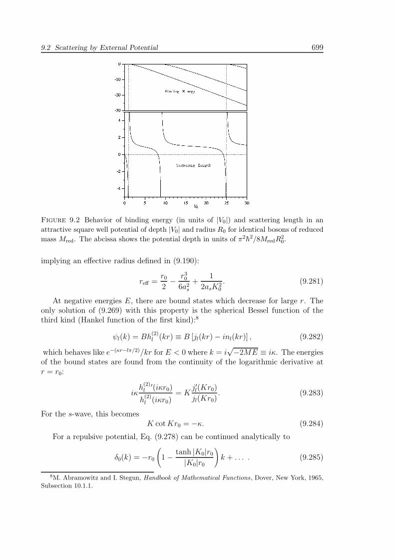
9.2 Scattering by External Potential 699
Figure 9.2 Behavior of binding energy (in units of |V0|) and scattering length in an
attractive square well potential of depth |V0| and radius R0 for identical bosons of reduced
mass Mred. The abcissa shows the potential depth in units of π2h2/8MredR20.
implying an effective radius defined in (9.190):
reff =r02− r30
6a2s+
1
2asK20
. (9.281)
At negative energies E, there are bound states which decrease for large r. Theonly solution of (9.269) with this property is the spherical Bessel function of thethird kind (Hankel function of the first kind):8
ψl(k) = Bh(2)l (kr) ≡ B [jl(kr)− inl(kr)] , (9.282)
which behaves like e−(κr−lπ/2)/kr for E < 0 where k = i√−2ME ≡ iκ. The energies
of the bound states are found from the continuity of the logarithmic derivative atr = r0:
iκh(2)l
′(iκr0)
h(2)l (iκr0)
= Kj′l(Kr0)
jl(Kr0). (9.283)
For the s-wave, this becomesK cotKr0 = −κ. (9.284)
For a repulsive potential, Eq. (9.278) can be continued analytically to
δ0(k) = −r0(
1− tanh |K0|r0|K0|r0
)
k + . . . . (9.285)
8M. Abramowitz and I. Stegun, Handbook of Mathematical Functions , Dover, New York, 1965,Subsection 10.1.1.

700 9 Scattering and Decay of Particles
In the hard-core limit V0 →∞, this yields an s-wave scattering length
as = −r0, (9.286)
and a vanishing effective range.For the hard-core potential, equation (9.205) has been solved [3]. The lth partial
wave amplitude is
Tl(k′, k;E) = −(−1)l 2πh2a
(2πM)3
k2E − k′2k2 − k′2 ka jl(k
′a)jl+1(ka) + (k ↔ k′)
− kEah(2)l+1(ka)
h(2)l (ka)
jl(k′)jl(k)
, (9.287)
where kE ≡√2ME/h.
9.3 Two-Particle Scattering
Usually, the final state has two or more particles leaving the interaction zone. Theinteraction energy is an integral over some local interaction density
V =∫
d3x Hint(x), (9.288)
integrated over all space at a fixed time x0 = t = 0. In this case, the matrix elementsof the potential factorizes as
〈p′|V |p〉 =∫
d3x 〈p′|eipxHint(0)e−ipx|p〉 = V δp′ p〈p′|Hint(0)|p〉, (9.289)
where p and p′ are the sum over all initial and final momenta, respectively. Thus thematrix elements of V always carry a δp′ p-factor that ensures total momentum con-servation. The same thing is true for the T -matrix Tp′p. This factor is customarilyremoved by defining the so-called t-matrix
Tp′p = V δp′ p tp′p. (9.290)
The Born approximation is now
tp′p ≈ 〈p′|Hint(0)|p〉. (9.291)
Replacing the Kronecker δ for momentum conservation by its continuum limit,
δp′ p →(2π)3
Vδ(3)(p′ − p),
we can write (9.290) as
Tp′p = (2π)3δ(3)(p′ − p) tp′p, (9.292)

9.3 Two-Particle Scattering 701
i.e., the matrix elements (9.130) of the S-matrix become
〈p′|S|p〉 = 〈p′|p〉 − i(2π)4δ(4)(p′ − p) tp′p. (9.293)
In a world of a finite volume V existing for a finite time T , the probability ofgoing from an initial state p to a final state p′ is given by the absolute square of(9.293). By analogy with (9.233), we have
δ(4)(p)∣
∣
∣
p=0=∫
d4p
(2π)4eipx
∣
∣
∣
∣
∣
p=0
=TV
(2π)4, (9.294)
so that we obtain the transition rate [compare (9.234)]. Thus we can write (9.232)as
P = TV (2π)4δ(4)(p′ − p)|tp′p|2. (9.295)
This has to be summed over all final particle states, and we obtain the rate
dP
dt= V
∑
final states
(2π)4δ(4)(p′ − p)|t f i|2. (9.296)
We have changed the notation for the t-matrix tp′p and written it as t f i to emphasizethe validity for a more general initial state | i〉 and a larger variety of possible finalstates |f 〉.
If the particles 1′, 2′, . . . , n′ leave the interaction zone, the sum over all final statesin a volume V consists of an integral over the phase space
∑
p′
1,p′
2,...
= V n∫ d3p′1
(2π)3
∫ d3p′2(2π)3
· · ·∫ d3p′n
(2π)3, (9.297)
and (9.296) becomes
dP
dt= V n+1
∫
d3p′1(2π)3
∫
d3p′2(2π)3
· · ·∫
d3p′n(2π)3
(2π)4δ(4)(p′ − p)|t f i|2, (9.298)
where p = p1 + p2 and p′ = p′1 + p′2 + . . . + p′n. By dividing out the current densityof the incoming particles j, we find from this the cross section
σ =dP
dt
1
j. (9.299)
By omitting some of the final-state integrations, we may extract from this anydesired differential cross section.
9.3.1 Center-of-Mass Scattering Cross Section
Let us assume the collision to take place in the center-of-mass frame with zero totalmomentum and p = p1 = −p2 and a total energy ECM. Then the δ-function fixes
702 9 Scattering and Decay of Particles
p′ = p′1 = −p′
2, and the equality of the total energies before and after the collisionimplies that
E ′1 + E ′
2 = E1 + E2 = ECM. (9.300)
In order to be more explicit we have to distinguish the case of nonrelativistic andrelativistic particles. It is useful to treat the relativistic case first and obtain thenonrelativistic result by going to the limit of small velocities. In the relativisticcase with initial momenta pCM = p1 = −p2, final momenta p′
CM = p′1 = −p′
2, andenergies
E1,2 =√
p2CM +M21,2, E ′
1,2 =√
p′CM2 +M ′
1,22, (9.301)
the δ-function for the total energy reads, in the center-of-mass frame, with zero totalmomentum
δ(
√
p′CM2 +M ′
12 +
√
p′CM2 +M ′
22 −ECM
)
. (9.302)
This is zero unless p′ makes the argument zero, which happens at
p′CM =1
2MI (M,M ′
1,M′2) , (9.303)
where
I(M,M1,M2) ≡√
M2 − (M1 +M2)2√
M2 − (M1 −M2)2 (9.304)
and
ECM =M ≡√s. (9.305)
The energy ECM is equal to the total mass, since the momentum in the center-of-massframe is zero. Another notation for M is
√s, where s is the so-called Mandelstam
variable. The individual energies of the two particles are
E1,2 =√
p2CM −M21,2 =
1
2M
[
M2 ±(
M21 −M2
2
)]
,
E ′1,2 =
√
p′CM2 −M ′2
1,2 =1
2M
[
M2 ±(
M ′21 −M ′2
2
])
. (9.306)
To evaluate the momentum integral over the δ-function (9.302), we use the formula
δ (f(p′)− f(p′CM)) = [f ′(p′)]−1δ(p′ − p′CM) (9.307)
to write
δ(
√
p′2 +M ′12 +
√
p′2 +M ′22 − ECM
)
= [(∂/∂p′) (E ′1 + E ′
2)]−1δ(p′ − p′CM)
=E ′
1E′2
p′CM (E ′1 + E ′
2)δ(p′ − p′CM) =
E ′1E
′2
p′CMECM
δ(p′ − p′CM). (9.308)

9.3 Two-Particle Scattering 703
Then we obtain from (9.298) the total rate of scattered relativistic particles
dP (t)
dt=
V 3
(2π)2p′CME
′1E
′2
ECM
∫
dΩ|t f i|2. (9.309)
Since the t-matrix elements depend, in general, on more than just the initial andfinal total momenta p and p′, they have been denoted generically by t f i.
The initial current density is given by the relative velocity between two incomingparticles in the center-of-mass frame:
j =(
p1E1− p2E2
)
1
V=pCMECM
E1E2
1
V. (9.310)
Dividing dP (t)/dt by j as demanded by (9.299) and omitting the integrationover the solid angle in (9.309), we obtain the differential cross section in the centerof mass:
dσ
dΩCM
=1
(2π)2p′CM
pCM
1
E2CM
E ′1E
′2E1E2V
4|t f i|2. (9.311)
It is useful to realize that the combination of incoming currents and energies j×2V E1E2 is a Lorentz-invariant quantity coinciding with I(M,M1,M2) of Eq. (9.304).This follows immediately by inserting (9.303) into (9.310):
j =1
2V E1E2I(M,M1,M2). (9.312)
Thus we can write down an explicit formula for the cross section (9.299) in anyframe of reference:
σ =2V E1E2
I(M,M1,M2)V n
∫ d3p′1(2π)3
∫ d3p′2(2π)3
· · ·∫ d3p′n
(2π)3δ(4)(p′ − p)|t f i|2. (9.313)
9.3.2 Laboratory Scattering Cross Section
In most experiments, the directly measured quantity is the laboratory cross sectionwhere an initial particle of momenta |p1| = pL and energy
EL ≡ (E1)Lab =√
p2L +M21 (9.314)
hits the particle 2 at rest. Then the incoming current is
j =pLELV
=vLV, (9.315)
rather than (9.310). The cross section of two particles going into two particles inthe laboratory is from (9.298) and (9.299):
σ =∫
d3p′1V
(2π)3d3p′2V
(2π)3(2π)4δ(4)(p′ − p)|t f i|2
V
j. (9.316)

704 9 Scattering and Decay of Particles
The δ-function for the total energy depends on the final laboratory momenta p1L ≡|p1L|, p2L ≡ |p2L| as follows:
δ(
√
p′1L2 +M ′
12 +
√
p′2L2 +M ′
22 − EL −M2
)
. (9.317)
In contrast to the center-of-mass frame, the final momenta p′1L and p′2L are nolonger equal, which complicates the further evaluation. We want to express them asfunctions of the initial energy and the scattering angle θL. For this, some kinematicconsiderations are necessary.
The total mass introduced in (9.305) is given by the Poincare-invariant quantity
M2 = s ≡ (p1 + p2)2 =M2
1 +M22 + 2M2EL. (9.318)
Solving this we obtain the invariant expressions
EL =(
M2 −M21 −M2
1 −M22
)
/2M2 (9.319)
pL = I (M,M1,M2) /2M2. (9.320)
Observe that by inserting the last equation into the frame-independent expression(9.312), we find the correct current (9.315) in the laboratory frame. The relationbetween the laboratory and center-of-mass energies is
E1CM =M2EL +M2
1√
M21 +M2
2 + 2ELM2
, (9.321)
E2CM =M2EL +M2
2√
M21 +M2
2 + 2ELM2
. (9.322)
The relation between the laboratory and the center-of-mass momenta is
pCM = pLM1
√
M21 +M2
2 + 2ELM2
. (9.323)
The relation between the scattering angles in the two frames of reference is moreinvolved. To find it, we consider a Lorentz invariant quantity that is formed fromthe momentum transfer, the so-called Mandelstam variable t:
t ≡ (p1 − p′1)2 =M21 +M ′
12 + 2(p1p
′1 − E1E
′1). (9.324)
In either frame, the scattering angles appear in the scalar product p1p′1 = p1p
′1 cos θ.
A calculation in the center-of-mass frame leads to the formula
cos θCM =1
2pCMp′CM
(t−M21 −M ′
12 + 2E1CME
′1CM)
=1
I(M,M1,M2)I(M,M ′1,M
′2)
(9.325)
× [M4 +M2(2t−M21−M2
2−M ′12−M ′
22) + (M2
1−M22 )(M
′12−M ′
22)].

9.3 Two-Particle Scattering 705
In the laboratory frame, we take advantage of the fact that p2 = (M2, 0) andcalculate t using energy-momentum conservation as
t = (p1 − p′1)2 = (p′2 − p2)2 =M ′22 +M2
2 − 2M2E′2L. (9.326)
It is convenient to introduce another Lorentz-invariant Mandelstam variable u as
u ≡ (p1 − p′2)2 = (p′1 − p2)2 =M22 −M ′
12 − 2M2E
′1L. (9.327)
The three Mandelstam variables s, t, u have the sum
s+ t+ u =M21 +M2
2 +M ′12 +M ′
2. (9.328)
This implies that all different kinematical configurations of a two-body scatteringprocess can be represented in an invariant way by a point in an equilateral triangleof height M2
1 +M22 +M ′
12 +M ′
22, the so-called Mandelstam triangle. The heights
over the three sides represent the quantities s, t, u.Similar considerations can be made for the process of a particle decaying into
three particles. Then a Poincare-invariant way of picturing the distribution of thefinal products in a Mandelstam triangle is known as Dalitz plot .
The laboratory energy of all particles can be calculated from (9.319) and
E2L =1
M2(M2
2 +M ′22 − t), (9.329)
E ′1L =
1
M2
(M22 +M ′
12 − u). (9.330)
By evaluating the invariant (9.324) in the laboratory frame, we find the scatteringangle in this frame:
cos θL =(M4 −M2
1 −M22 )(M
22 +M ′
12 − u) + 2M2
2 (t−M21 −M ′
12)
I(M,M1,M2)I(M,M ′1,M
′2)
. (9.331)
The argument of the total energy δ-function (9.317) requires the knowledge ofthe momenta p′1, p
′2 of the final particles as a function of the initial energy EL and
the scattering angle θL. These can now be calculated as follows. From (9.318) wefind the invariant M as a function of EL. This is inserted into (9.331) to obtain theinvariant t as a function. Together with (9.328), this fixes the invariant u. Insertedinto Eqs. (9.330), we find the final energy E ′
1L, and from energy conservation alsoE ′
2L. These determine the final momenta.It is useful to generalize the definition of the scattering amplitude f that was
introduced in (9.249) for the scattering of a nonrelativistic particle on an externalpotential. The generalization holds also in present case of two relativistic particlesscattering on each other in the center-of-mass frame. . As before, we define f sothat its absolute square gives the differential cross section:
dσ
dΩCM
= |f |2. (9.332)

706 9 Scattering and Decay of Particles
Then we see from (9.311) that f should be identified with
f = − 1
2π
√
p′CM
pCM
1
ECM
√
V 4E ′1E
′2E1E2 t f i. (9.333)
In the case of elastic scattering on a very heavy particle of mass M2 (choosing thesecond perticle to be the heavier one), this reduces back to the original definition.
In a more general scattering process in which two particles collide and producea final state with n particles, the production cross section is given by
σ f i =V
j
n∏
i=1
[
∫ d3piV
(2π)
]
(2π)4δ(4)(p′ − p)|t f i|2, (9.334)
with the prefactor V/j = V 2E1E2/pCMECM, as given by (9.310).
Scattering processes in a center-of-mass frame with zero total momentum can beobserved directly in colliding beam experiments. There one has two beams impingingalmost with opposite momenta (see Fig. 9.3). If Vint is the volume of the intersecting
Figure 9.3 Geometry of particle beams in a collider. The angle of intersection α is
greatly exaggerated. The intersection defines the interaction volume Vint.
zone, the so-called interaction volume, and n1, n2 are the particle densities in thetwo beams (particles per unit volume), the so-called luminosity of the colliding beamis obtained from the relative velocity vrel by forming the product
L = vrelVintn1n2 =I(M,M1,M2)
2E1E2Vintn1n2. (9.335)
The rate of particle scattering is obtained by multiplying this with the differentialcross section dσ/dΩCM:
dN
dtdΩCM= L
dσ
dΩCM. (9.336)
Note that the luminosity increases linearly if the beams are focused upon a smallerarea (since n1n2 increases like 1/area2 while Vint increases like area).
9.4 Decay 707
9.4 Decay
The decay rate of an unstable particle into two particles is directly given byEq. (9.298):
dP
dt= V 2
∫
d3p′1(2π)3
∫
d3p′2(2π)3
(2π)4δ(4)(p′ − p)|t f i|2. (9.337)
Evaluating this in the center-of-mass frame of the decaying particle yields
Γ =d
dtP (t) =
V 3
(2π)2p′CME
′1E
′2
M
∫
dΩ |t f i|2, (9.338)
where M is the mass of the initial particle. If the particle has spin s and decays intofinal spins s′1, s
′2, an unpolarized initial state and all possible final spin orientations
m′1 = −s′1, . . . , s′1 and m′
2 = −s′2, . . . , s′2 lead to an isotropic distribution, and wecan simplify (9.338) to
Γ =d
dtP (t) =
V 3
(2π)2p′CME
′1E
′2
M
4π
2s+ 1
∑
m′
1,m′
2
|t f i|2. (9.339)
9.5 Optical Theorem
The unitarity of the S-matrix (9.44),
SS† = S†S = 1, (9.340)
implies an important theorem for the imaginary part of the diagonal elements of theT -matrix. Writing
S f i = δ f i − i(2π)4δ(4) (pf − pi) t f i , (9.341)
we see that
−i(
tii − t†ii)
= −∑
f
t†if(2π)4δ(4) (pf − pi) t f i , (9.342)
where the sum runs over all possible many particle states. According to Eq. (9.333),the left-hand side is related to the imaginary part of the forward scattering amplitudefii as follows
2πECM
V 2E1E2Im fii = −
∑
n
n∏
i=1
[
∫
d3piV
(2π)3
]
(2π)4δ(4) (pf − p1) |t f i|2 . (9.343)
Now, the right-hand side, if divided by the relative current density j =pCMECM/E1E2V , is equal to 1/V times the sum over all cross sections σ f i, i.e.,

708 9 Scattering and Decay of Particles
it is equal to −j/V times the total cross section −(j/V )σtot [see (9.316)]. For theforward scattering amplitude fii this implies the simple relation
2π
pCM
fii = −σtot. (9.344)
This relation is referred to as the optical theorem (in reference to a theorem re-lating the total absorption of light to the imaginary part of the forward-scatteringamplitude).
9.6 Initial- and Final-State Interactions
Some inelastic scattering and decay processes are caused by a weak interactionHamiltonian Hw, which can be treated in Born approximation. This can happenwhile initial- and final states are still governed by strong interactions with a Hamil-tonian Hs. Suppose the total Hamiltonian contains these interactions additively,i.e.,
H = H0 + Vs + Vw. (9.345)
In specific applications, Hw may be the weak interaction of beta decay, say, and Hs
a combination of electromagnetic and strong interactions. Alternatively, Hw maybe an electromagnetic interaction, and Hs the strong interaction.
For time-independent interactions, the Møller operators are given by (9.32) andread explicitly
Ω(±) = UI (0,∓∞) = limt→∓∞
ei(H0+ˆV w+Vs)te−iH0t. (9.346)
The right-hand sides can obviously be decomposed into a product
UI (0,∓∞) = UIw (0,∓∞) UI,s (0,∓∞) , (9.347)
where
UIw (0,∓∞) = limt→∓∞
ei(H0+Vs+Vw)te−i(H0+Hs)t, (9.348)
UIs (0,∓∞) = limt→∓∞
ei(H0+Vs)te−iH0t. (9.349)
Thus we can write the Møller operators as
Ω(±) = Ω(±)w Ω(±)
s , (9.350)
withΩ(±)
w = UIw (0,∓∞) , Ω(±)s = UIw (0,∓∞) . (9.351)
Using this, we can express the scattering amplitude as follows:
Sfi = 〈f|UIs(∞, 0)SwUIs(0,−∞)|i〉, (9.352)
9.7 Tests of Time-Reversal Violations 709
where, by analogy with (9.42),
Sw ≡ UIw (∞,−∞) = Ω(−)w
†Ω(+)w . (9.353)
For a simple description of the effects of the initial- and the final-state interactionsit is convenient to introduce, in a slight variation of (9.114), the notation
| i(±)〉 ≡ UIs(0,∓∞)| i〉 = Ω(+)w | i〉, (9.354)
where the symbols (±) refer now to the activity of Hw in the time evolution. Thescattering matrix elements become
〈j|S| i〉 = 〈j(−)|Sw| i(+)〉. (9.355)
Under the assumption of a weak Vw, we replace Sw by its Born approximation andwrite
Sw ≈ −i∫ ∞
−∞dtVIw(t), (9.356)
where
VIw(t) ≡ ei(H0+Vs+Vw)tVwe−i(H0+Vs)t (9.357)
is the interaction representation of the weak interaction in the presence of the initial-and final-state interactions. The initial and final states are eigenstates of the opera-tor H0+ Vs [see (9.15)]. The integration over t in (9.356) can now be done in (9.356),and leads to a δ-function of energy conservation [recall the derivation of (9.130)], sothat
〈j|S| i〉 = 〈j| i〉 − 2πiδ(E ′ − E)〈j(−)|Vw| i(+)〉. (9.358)
For a local interaction which arises from an integral over an interaction density asin Eq. (9.288), we find that the initial- and final-state interactions are accounted forby the modified t-matrix
tp′p ≈ 〈p′(−)|Hint(0)|p(+)〉. (9.359)
For the amplitude of multiparticle scattering (9.296), the corresponding expressionis
tfi ≈ 〈f(−)|Hint(0)| i(+)〉. (9.360)
9.7 Tests of Time-Reversal Violations
If the Hamiltonian is invariant under time-reversal, the time translation operatorU(t, t0) fulfills the equation (7.123). This has the consequence that the scatteringoperator S of Eq. (9.42) satisfies
T †ST = S†. (9.361)

710 9 Scattering and Decay of Particles
To derive observable consequences from this, we first use the equations (7.118) and(7.119) to deduce trivially the equality for any matrix element between an initialstate |i〉, obtained by applying one or more particle creation operators upon thevacuum, and a final state |f〉, obtained likewise:
〈f|S|i〉 = 〈f|1AS|i〉∗. (9.362)
Invoking now time-reversal invariance by applying (9.361), we obtain
〈f|S|i〉 = 〈f|T †S†T |i〉∗ = 〈fT |S†|iT 〉∗ = 〈iT |S|fT 〉. (9.363)
Here |iT 〉 denotes the time-reversed version of the state |i〉, in which all creationoperators are replaced by the right-hand sides of (7.113), (7.322), etc. Thus momentaand spin directions are reversed, and there is a phase factor ηT for each particle.
9.7.1 Strong and Electromagnetic Interactions
Strong and electromagnetic interactions are time-reversal invariant. The matrixelements of the scattering operator S, the scattering amplitudes, satisfy the identity
〈pc, s3c;pd, s3d|S|pa, s3a;pb, s3b〉 = η〈−pa,−s3a;−pb,−s3b|S| − pc,−s3c;pd, s3d〉,(9.364)
with some phase factor η of unit norm. When calculating the unpolarized crosssection, we have to sum over the final states, and average over the initial states. Inthe center-of-mass frame, the cross section carries a phase-space factor p′CM/pCM ,the ratio of final and initial center-of-mass momenta. It has to be removed tocompare the squared amplitudes. Hence we obtain
dσ(ab→ cd)
dΩdσ(cd→ ab)
dΩ
=
(
pcdCM
pabCM
)2(2sc + 1)(2sd + 1)
(2sa + 1)(2sb + 1). (9.365)
This is called the principle of detailed balance. It is important for the thermalequilibrium of chemical reactions. This equation was used in 1951 to determine thespin of the pion from a reaction in which two protons collide and produce a pionand a deuteron9:
p+ p d+ π+. (9.366)
The principle of detailed balance says that
dσ(→)
dΩdσ(←)
dΩ
=3
4
q2π(2sπ + 1)
p2p. (9.367)
This relation was satisfied with sπ = 0.
9R.E. Marshak, Phys. Rev. 82, 313 (1951); W.B. Cheston, Phys. Rev. 83, 1118 (1951); R.Durbin, H. Loar, and J. Steinberger, Phys. Rev. 83, 646 (1951); D.L. Clark, A. Roberts, and R.Wilson, Phys. Rev. 83, 649 (1951).

9.7 Tests of Time-Reversal Violations 711
9.7.2 Selection Rules in Weak Interactions
Consider a one-particle state |i〉 prepared by strong and electromagnetic interactions,which decays into a several-particle state |b〉 via weak interactions. Let O be anobservable which changes sign under time reversal:
OT = −O. (9.368)
Consider the expectation value of O a long time after the decay. It is given by
〈O〉 = 〈i|U(−∞,∞) ∧OU(∞,−∞)|i〉 = 〈i|S†OS|i〉. (9.369)
Using the antiunitarity of the time-reversal operator as expressed by Eqs. (7.118)and (7.119), the right-hand side can be rewritten as
〈i|S†OS|i〉 = 〈i|1AS†OS|i〉∗ = 〈i|T †T S†OS|i〉∗. (9.370)
Time-reversal invariance (9.361) brings this to
〈i|T †SOT S†T |i〉∗ = 〈iT |SOT S
†|iT 〉∗. (9.371)
Since O was assumed to be an observable, the expectation is real, and we can dropthe complex conjugation at the end. This leaves us with the relation
〈O〉 = 〈i|S†OS|i〉 = 〈iT |SOT S†|iT 〉. (9.372)
If the decay is very slow, the scattering operator can be replaced by its Born ap-proximation
S ≈ SB ≡ i∫ ∞
−∞dtVIw(t), (9.373)
which is a Hermitian operator, up to a factor i (the direct term in (9.341) does notcontribute to a decay process). But then (9.372) becomes
〈O〉 = 〈i|SBOSB|i〉 = 〈iT |SBOT SB|iT 〉. (9.374)
If the initial particle is spinless, then
|iT 〉 = ηT |i〉, |ηT | = 1. (9.375)
Together with (9.368), this implies
〈O〉 = 0. (9.376)
Thus, in a weak decay process, the expectation value of an observable that changessign under time-reversal, is zero. Note that this result is independent of the phaseηT of the decaying particle.
Without the weakness assumption, the change to the Hermitian conjugates ofthe scattering operators in (9.372) would have prevented us from any conclusion.

712 9 Scattering and Decay of Particles
Historically, the invariance under time reversal of weak interactions was appar-ently assured by the weak decays
K+ −−−→ π0 + µ+ + ν, K− −−−→ π0 + µ− + ν. (9.377)
The outcoming muon was initially found to have no average polarization orthogonalto the production plane formed by the momenta pµ and pπ, i.e., the operator O =µ ·(pµ× pπ) had no measurable expectation value. Since this operator is odd under
time reversal, the vanishing of 〈O〉 seemed to confirm time-reversal invariance.10
However, as it turned out later, the breakdown of time-reversal invariance in weakinteractions is much too small to be detected by a polarization experiment. Thereexists a much more sensitive experiment which shows the violation dramatically:the K0-K0 meson system. This will be discussed later.
9.7.3 Phase of Weak Amplitudes from Time-Reversal Invariance
If a particle decays weakly into two final particles, time-reversal invariance fixesthe phase of the decay amplitude. Let us assume that the final-state interaction ispurely elastic, i.e., that there are no other decay channels caused by the final-stateinteractions, then a weak decay can be treated in lowest-order perturbation theory.It has the amplitude
tba = 〈f(−)|Hw|i(+)〉, (9.378)
where the labels (±) indicate the states defined in Section 9.6, containing the fulleffect of the initial- and final-state interactions. Under the assumption of time-reversal invariance of the weak interactions, we find
〈f(−)|Hw|i(+)〉 = 〈iT (−)|Hw|fT (+)〉 = 〈fT (+)|Hw|iT (−)〉∗. (9.379)
If we choose the phase factors ηT of initial and final particles to be unity [see (4.226)],we obtain
〈f(−)|Hw|i(+)〉 = 〈fT (+)|Hw|iT (−)〉∗. (9.380)
The initial state is a stationary single-particle state if the weak interactions areignored. Hence
|i(+)〉 ≈ |i(−)〉. (9.381)
We now rotate the matrix element on the right-hand side in space by 180 degrees,we reverse, in the center of mass frame, momentum and spin directions, and bringthe time-reversed state back to the original form. Thus we obtain
〈b(−)|Hw|a(+)〉 = 〈b(+)|Hw|a(−)〉∗. (9.382)
10This possibility of testing time-reversal invariance of weak interactions was pointed out by J.J.Sakurai, Phys. Rev. 109, 980 (1958). See also M. Gell-Mann and A.H. Rosenfeld, Ann. Rev.Nucl. Sci. 7, 407 (1957), Appendix A.
Appendix 9A Green Function in Arbitrary Dimensions 713
The amplitudes with + and − interchanged differ by a pure phase factor, that isprecisely the scattering amplitude for the two-particle scattering in their final state:
〈b(−)|Hw|a(+)〉 = e2iδ〈b(+)|Hw|aT (−)〉. (9.383)
The pure-phase nature is a consequence of the elasticity assumption of the two-particle scattering process. Together with (9.382), this fixes the phase:
〈b(∓)|Hw|a(+)〉 = const .× eiδ. (9.384)
This equation has many applications in phenomenological analyses [5].
Appendix 9A Green Function in Arbitrary Dimensions
In D dimensions, the Green function (9.138) in the scattered wave (9.136) of the Lippmann-Schwinger equation has the following form:
〈x|G0(E)|x′〉 = −2Mih
∫
dDp
(2πh)Deip(x−x′)/h
p2 − p2E. (9A.1)
The momentum integral has been calculated in Section 1.12 (also 9.1) of Ref. [2], for E > 0 yielding
〈x|G0(E)|x′〉 = Mπ
h
kD−2E
(2π)D/2
H(1)D/2−1(kE |x− x′|)(kE |x− x′|)D/2−1
, (9A.2)
where kE ≡ pE/h =√
2M(E + iη)/h, and H(1)(z) is the Hankel function, whose leading large-zbehavior is
H(1)ν ≈
√
2
πzei(z−πν/2−π/4), (9A.3)
thus reproducing the previous result (9A.1) for D = 3.In D = 1 dimension, the expression (9A.2) reduces to
〈x|G0(E)|x′〉 = M
hkEeikE |x−x′|, (9A.4)
so that the Lippmann-Schwinger equation (9.134) in one dimension reads
〈x|ψ(+)k 〉 =
1
L1/2
[
eikx + iM
h2kEeikE |x−x′|
∫ ∞
−∞
dxV (x′)〈x′|ψ(+)k 〉
]
, (9A.5)
where kE =√
2M(E + iη) is equal to the wave number k of the incoming particles.As a simple application, consider the case of a δ-function potential
V (x) =h2
Mlδ(x), (9A.6)
where (9A.5) becomes
〈x|ψ(+)k 〉 =
1
L1/2
[
eikx +1
ikleik|x|
∫ ∞
−∞
〈0|ψ(+)k 〉
]
. (9A.7)
Setting x = 0 on the left-hand side determines
〈0|ψ(+)k 〉 =
1
L1/2
ikl
ikl − 1, (9A.8)

714 9 Scattering and Decay of Particles
and Eq. (9A.7) yields the fully interacting wave function
〈x|ψ(+)k 〉 =
1
L1/2
[
eikx +1
ikl− 1eik|x|
]
. (9A.9)
The corresponding states |ψ(−)k 〉 are
〈x|ψ(−)k 〉 = 1
L1/2
[
e−ikx +1
−ikl− 1e−ik|x|
]
. (9A.10)
In the negative-x regime, the second wave runs to the left and its prefactor is the reflection
amplitude
r =1
ikl − 1. (9A.11)
At positive x, the two exponentials run both to the right and the common prefactor
t =ikl
ikl− 1(9A.12)
is the transmission amplitude. The unitarity relation for this process is |r|2 + |t|2 = 1.For an attractive δ-function, there is a bound-state pole at kB = 1/|l|, corresponding to the
energy
εB = − h2k2B2M
= − h2
2l2M= −g
2M
2. (9A.13)
It is easy to verify that 〈x|ψ(±)k 〉 satisfies the Schrodinger equation
[
− h2∂2x2M
+h2
Mlδ(x)− E
]
〈x|ψ(±)k 〉 = 0, (9A.14)
with the jump property of the solution at the position of the δ-function
h2∂x2M
[〈0+|ψ(±)k 〉 − 〈0−|ψ
(±)k 〉] =
h2
Ml〈0|ψ(±)
k 〉. (9A.15)
Let us also calculate the matrix elements of the resolvent operator (9.57), i.e., the Greenfunction
〈x|G(E)|x′〉 = 〈x| ih
E − H + iη|x′〉. (9A.16)
It has the spectral representation
〈x|G(E)|x′〉 =∫ ∞
−∞
dk
2π
ih
E − Ek + iη〈x|ψ(±)
k 〉〈ψ(±)k |x′〉. (9A.17)
Performing the integral over k we find, from the residue at kE :
〈x|G(E)|x′〉 = M
hkE
[
eikE |x−x′| +1
ikEl − 1eikE(|x|+|x′|)
]
. (9A.18)
This is related to the free Green function (9A.4) via Eq. (9.58).The Green function (9A.18) can also be obtained with the help of the Wronski method11 by
combining the two independent solutions
f1(x) =√L〈x|ψ(+)
kE〉, f2(x) = f∗
1 (x) (9A.19)
11See Subsection 3.2.1 in the textbook [2].
Appendix 9B Partial Waves in Arbitrary Dimensions 715
of the homogeneous Schrodinger equation (H − E)f(x) = 0 in the form
〈x|G(E)|x〉 = 〈x| ih
E − H|x′〉 = 2Mi
h
1
W (x, x)[Θ(x−x′)f1(x)f2(x′) + Θ(x′−x)f1(x′)f2(x)], (9A.20)
where W (x, x) is the Wronski determinant
W (x, x) ≡ f ′1(x)f2(x)− f1(x)f ′
2(x′). (9A.21)
Indeed, applying the operator E − H = E + h∂2x/2M to (9A.20), we obtain ihδ(x− x′).For the free system where f1(x) = eikEx, f2(x) = e−ikEx, and W (x, x) = 2ikE , this formula
reproduces the above result (9A.4):
〈x|G0(E)|x〉 = 2Mi
h
1
W (x, x)f1(x>)f2(x<) =
M
hkEeikE |x−x′|. (9A.22)
In the presence of the δ-potential, where the Wronski determinant is calculated from the solutions(9A.19) as
W (x, x) =2ik2El
kE l + i, (9A.23)
the general formula (9A.20) yields
〈x|G(E)|x〉 = 〈x| ih
E − H|x′〉 = M
hkE
[
eikE |x−x′| − 1
1−ikEleikE(|x|+|x′|)
]
. (9A.24)
From this, we find the bilocal density of states
〈x|ρ(E)|x′〉= 1
2πh〈x|[G(E+iη)−G(E−iη)]|x〉= M
2πh2kE
[(
eikE(x−x′)+1
ikEl−1eikE(|x|+|x′|)
)
+c.c.
]
.
(9A.25)
Integrating this over all energies in the continuum, i.e., by forming∫∞
0 dE = h2∫∞
−∞ kEdkE/M ,we obtain
∫ ∞
0
dE〈x|ρ(E)|x′〉 = δ(x− x′)−Θ(−l) 1
−l e−(|x|+|x′|)l. (9A.26)
According to Eq. (9A.17), the same quantity is equal to∫ ∞
0
dE
∫ ∞
−∞
dk
2π〈x|ψ(+)
k 〉δ(E − hk2/2M)〈ψ(+)k |x′〉 =
∫ ∞
−∞
dk
2π〈x|ψ(+)
k 〉〈ψ(+)k |x′〉. (9A.27)
Hence Eq. (9A.26), together with the contribution of the single bound state wave function 〈x|ψβ〉 =(1/√−l)e−|x|l, yields
∫ ∞
−∞
dk
2π〈x|ψ(+)
k 〉〈ψ(+)k |x′〉+ δ(−l)〈x|ψβ〉〈ψβ |x′〉 = δ(x− x′), (9A.28)
thus proving the completeness relation (9.62) of the states 〈x|ψ(+)k 〉 and 〈x|ψβ〉 = (1/
√−l)e−|x|l.
Appendix 9B Partial Waves in Arbitrary Dimensions
In D dimensions, the angular decomposition of the scattering amplitudes proceeds as follows. Forequal incoming and outgoing energies Ep′ = Ep, where |p′| = |p| = p, the T -matrix 〈p′|T |p〉 inEq. (9.129) has an expansion
〈p′|T |p〉 =(2π)D
V
∞∑
l=0
Tl(p)∑
m
Ylm(p′)Ylm(p), (9B.1)

716 9 Scattering and Decay of Particles
where Ylm(p) are the hyperspherical harmonics associated with the momentum direction p. Theygeneralize (4F.1), and their precise form is somewhat tedious to write down. Here we onlyrecall that their magnetic quantum numbers form a D − 2-dimensional vector of eigenvalues(m1,m2, . . . ,mD−2) running through the number
dl =(2l+D − 2)(l +D − 3)!
l!(D − 2)!(9B.2)
of different values for each l. The orthogonality (4F.3) becomes now:
∫
d2pY ∗l′m′(p)Ylm(p) = δl′lδm′m, (9B.3)
where∫
dD−1p denotes the integral over the surface of a unit sphere in D dimensions:
∫
dD−1p = SD ≡2πD/2
Γ(D/2). (9B.4)
The spherical harmonics are matrix elements of eigenstates |lm〉 of angular momentum [recall(4.846)] with localized states |p〉 on the unit sphere:
〈p|lm〉 ≡ Ylm(p). (9B.5)
The latter are orthogonal:〈p′|p〉 = δ(D−1)(p′ − p), (9B.6)
where δ(D−1)(p′ − p) is the δ-function on a unit sphere.The addition theorem (23.12) for the spherical harmonics is replaced by
2l +D − 2
D − 2
1
SDC
(D/2−1)l (p′ · p) =
∑
m
Ylm(p′)Y ∗lm(p), (9B.7)
where the functions C(α)l (cosϑ) are the hyperspherical Gegenbauer polynomials, theD-dimensional
versions of the Legendre polynomials Pl(cos θ) in Eq. (4F.7).The Gegenbauer polynomials are related to Jacobi polynomials, which are defined in terms of
hypergeometric functions by12
P(α,β)l (z) ≡ 1
l!
Γ(l + 1 + β)
Γ(1 + β)F2,1(−l, l+ 1 + α+ β; 1 + β; (1 + z)/2). (9B.8)
The relation is13
C(ν)l (z) =
Γ(2ν + l)Γ(ν + 1/2)
Γ(2ν)Γ(ν + l + 1/2)P
(ν−1/2,ν−1/2)l (z). (9B.9)
Thus we can write
C(ν)l (z) =
1
l!
Γ(l + 2ν)
Γ(2ν)F2,1(−l, l+ 2ν; 1/2 + ν; (1 + z)/2). (9B.10)
For D = 2 and 3, one has14
limν→0
1
νC
(ν)l (cosϑ) =
1
2lcos lϑ, (9B.11)
12M. Abramowitz and I. Stegun, op. cit., Formula 15.4.6.13Ibid., Formula 15.4.5.14I.S. Gradshteyn and I.M. Ryzhik, op. cit., Formula 8.934.4.
Appendix 9B Partial Waves in Arbitrary Dimensions 717
C(1/2)l (cosϑ) = P
(0,0)l (cosϑ) = Pl(cosϑ). (9B.12)
The partial-wave expansion (9B.1) becomes, in D dimensions:
〈p′|T |p〉 =
∞∑
l=0
Tl(p)2l +D − 2
D − 2
1
SDC
(D/2−1)l (p′ · p). (9B.13)
A similar expansion for the S-matrix (9.130) requires expanding the scalar product 〈p′|p〉 = δp′,p
into partial waves. In a large volume V , we replace this by (2π)Dδ(D)(p′ − p)/V . The δ-functionis decomposed into a directional and a radial part
δp′,p =(2π)D
Vδ(D)(p′ − p) = δ(D−1)(p′ − p)
(2π)D
V
1
pD−1δ(p′ − p). (9B.14)
The directional δ-function on the right-hand side has a partial-wave expansion which is the com-pleteness relation [compare (9.161] for the states |l m〉,
∞∑
l=0
∑
m
|lm〉〈lm| = 1, (9B.15)
evaluated between the localized states |p〉 on the unit sphere. Using the matrix elements (9B.5)and the orthogonality relation (9B.6), we find from (9B.15):
δ(D−1)(p′ − p) =
∞∑
l=0
l∑
m
Ylm(p′)Y ∗lm(p). (9B.16)
The radial part of (9B.14) can be rewritten as
(2π)D
V
1
pD−1δ(p′ − p) = (2π)D
V
1
pD−1
dE
dpδ(E′ − E) =
(2π)D
V
1
ρEδ(E′ − E), (9B.17)
where
ρE ≡pD−1
dE/dp. (9B.18)
It allows us to rewrite the sum over all momentum states as follows:
∑
p
=
∫
dDpV
(2π)D=
V
(2π)D
∫
dD−1p
∫
dE ρE . (9B.19)
Thus we find the expansion
〈p′|p〉 = δp′,p =(2π)D
V
∞∑
l=0
∑
m
Ylm(p′)Ylm(p)1
ρEδ(E′ − E). (9B.20)
In a partial-wave expansion for the S-matrix (9.130), the overall δ-function for the energyconservation is conventionally factored out and one writes:
〈p′|S|p〉 =(2π)D
V
1
ρEδ(E′ − E)
∞∑
l=0
Sl(p)∑
m
Ylm(p′)Ylm(p). (9B.21)
The relation between the partial-wave scattering amplitudes Sl(p) and those of the T -matrix isagain given by (9.168). The only change in D dimensions appears in ρE which acquires the form(9B.18).
718 9 Scattering and Decay of Particles
In order to show this we use the expansion formula corresponding to (9.173),
eih cos∆ϑ =
∞∑
l=0
al(h)l +D/2− 1
D/2− 1
1
SDC
(D/2−1)l (cos∆ϑ), (9B.22)
where
al(h) ≡ (2π)D/2h1−D/2ilJl+D/2−1(h). (9B.23)
The expansion (9B.22) follows from the completeness of the polynomials C(ν)l (cosϑ) at fixed ν,
using the integration formulas15
∫ π/2
−π/2
dϑ sinν ϑ eh cosϑC(ν)l (cosϑ) = π
21−νΓ(2ν + l)
l!Γ(ν)h−νIν+l(h), (9B.24)
∫ π/2
−π/2
dϑ sinν ϑC(ν)l (cosϑ)C
(ν)l′ (cosϑ) = π
21−2νΓ(2ν + l)
l!(l + ν)Γ(ν)2δll′ . (9B.25)
We now use (9B.22) to expand the incoming free-particle wave
〈x|p〉 =1√Veipx =
∞∑
l=0
ψl(pr)
l∑
m
Ylm(x)Ylm(p)
=
∞∑
l=0
ψl(pr)l +D/2− 1
D/2− 1
1
SDC
(D/2−1)l (x · p), (9B.26)
where r ≡ |x|, andψl(pr) =
1√Val(pr). (9B.27)
Far from the scattering region, the spherical Bessel functions have the asymptotic behavior
Jν(z)→√
2
πzsin(z − νπ/2 + π/4), (9B.28)
implying for the partial waves [compare (9.178)]
ψl(pr) =1√Vil 2 (2π)(D−1)/2 sinpr − π[l/2− (D − 3)/4]
(pr)(D−1)/2. (9B.29)
We shall now calculate the asymptotic form of the outgoing waves. The second term of theLippmann-Schwinger equation (9.131) yields the scattered wave, which reads in configuration space
〈x|p〉sc =∫
dDp′V
(2π)D〈x|p′〉 1
E − E′ + iη〈p′|T |p〉. (9B.30)
Inserting here the partial-wave decompositions (9B.1) and (9B.26), we find
∫
dDp′V
(2π)D〈x|p′〉 1
E − E′ + iη〈p′|T |p〉
=1√V
∞∑
l=0
∑
m
Ylm(x′)Ylm(p)
∫ ∞
0
dp′ p′D−1 al(p′r)Tl(p)
E − E′ + iη, (9B.31)
15I.S. Gradshteyn and I.M. Ryzhik, op. cit., Formulas 7.321 and 7.313.
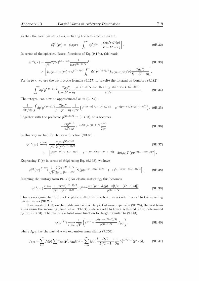
Appendix 9B Partial Waves in Arbitrary Dimensions 719
so that the total partial waves, including the scattered waves are
ψtotl (pr) =
[
ψl(pr) +
∫ ∞
0
dp′ p′D−1 ψl(p′r)Tl(p)
E − E′ + iη
]
. (9B.32)
In terms of the spherical Bessel functions of Eq. (9.174), this reads
ψtotl (pr) =
1√V2(2π)(D−1)/2 1
(pr)(D−3)/2il (9B.33)
×[
jl+(D−3)/2(pr) + p(D−3)/2
∫ ∞
0
dp′ p′(D+1)/2 jl+(D−3)/2(p′r)
Tl(p′)
E − E′ + iη
]
.
For large r, we use the asymptotic formula (9.177) to rewrite the integral as [compare (9.182)]
∫ ∞
0
dp′ p′(D+1)/2 Tl(p′)
E − E′ + iη
eip′r−π[l/2−(D−3)/4]−e−ip′r−π[l/2−(D−3)/4]
2ip′r. (9B.34)
The integral can now be approximated as in (9.184):
1
dE/dp
∫
dp′ p′(D+1)/2 Tl(p′)
p− p′ + iη
1
2ip′r
(
eipr−π[l/2−(D−3)/4] − e−ipr−π[l/2−(D−3)/4])
. (9B.35)
Together with the prefactor p(D−3)/2 in (9B.33), this becomes
−2πpD−1
dE/dpe−iπl/2eiπ(D−3)/4 e
ipr
2pr. (9B.36)
In this way we find for the wave function (9B.33):
ψtotl (pr)
r→∞−−−→ 1√
V
2(2π)(D−2)/2
2i(pr)(D−1)/2(9B.37)
×[
eipr−π[l/2−(D−3)/4]−e−ipr−π[l/2−(D−3)/4]−2πiρE Tl(p)eiπ(D−3)/4eipr]
.
Expressing Tl(p) in terms of Sl(p) using Eq. (9.168), we have
ψtotl (pr)
r→∞−−−→ 1√
V
2(2π)(D−1)/2
2i(pr)(D−1)/2
[
Sl(p)ei(pr−π(D−3)/4)−(−1)le−ip(pr−π(D−3)/4)
]
. (9B.38)
Inserting the unitary form (9.171) for elastic scattering, this becomes
ψtotl (pr)
r→∞−−−→ 1√
V
2(2π)(D−1)/2
p(D−1)/2ileiδl(p)
sinpr + δl(p)−π[l/2− (D−3)/4]r(D−1)/2
. (9B.39)
This shows again that δl(p) is the phase shift of the scattered waves with respect to the incomingpartial waves (9B.29).
If we insert (9B.33) on the right-hand side of the partial wave expansion (9B.26), the first termgives again the incoming plane wave. The Tl(p)-terms add to this a scattered wave, determinedby Eq. (9B.33). The result is a total wave function for large r similar to (9.143):
〈x|p(+)〉−−−→r→∞
1√V
(
eipx +ei(pr−π(D−3)/4)
r(D−1)/2fp′p
)
, (9B.40)
where fp′p has the partial wave expansion generalizing (9.250):
fp′p =
∞∑
l=0
fl(p)∑
m
Ylm(p′)Ylm(p) =
∞∑
l=0
fl(p)l +D/2− 1
D/2− 1
1
SDC
(D/2−1)l (p′ · p), (9B.41)

720 9 Scattering and Decay of Particles
with
fl(p) = −(2π)(D+1)/2
p(D−1)/2ρETl(p) =
(2π)(D−1)/2
ip(D−1)/2[Sl(p)− 1] =
2(2π)(D−1)/2
p(D−1)/2eiδl(p) sin δl(p). (9B.42)
Taking the absolute square of this, and integrating over all directions of the final momentum p′,we find the partial wave decomposition of the total cross section:
σ =
∫
dp′ |fp′p|2 =
∞∑
l=0
fl(p)fl(p)∗∑
lm
∑
l′m′
Ylm(p′)Ylm(p)Y ∗lm′(p′)Y ∗
lm′(p)
=∞∑
l=0
|fl(p)|2l+D/2−1D/2− 1
1
SDC
(D/2−1)l (1) =
∞∑
l=0
|fl(p)|2l+D/2−1D/2− 1
1
SD
(l+D−3)!l!(D − 2)!
,
(9B.43)
where we have used the special value of the Gegenbauer function16
C(ν)l (1) =
(
l + 2ν − 1
l
)
. (9B.44)
Inserting (9B.42), the cross section decomposes as
σ =
∞∑
l=0
σl =4(2π)D−1
pD−1
∞∑
l=0
l+D/2−1D/2− 1
1
SD
(l+D−3)!l!(D− 2)!
sin2 δl(p). (9B.45)
In three dimensions, this reduces to (9.253).
Appendix 9C Spherical Square-Well Potential
in D Dimensions
For a square-well potential (9.268) in D dimensions, the radial Schrodinger equation (9.269) be-comes
d2
dr2+D − 1
r
d
dr+
[
k2E −l(l +D − 2)
r2
]
ψl(r) = 0, (9C.1)
whereK ≡
√
2M(E + V0)/h. (9C.2)
There is only one solution which is regular at the origin:
ψl(r) =A
(Kr)D/2−1JD/2−1+l(Kr), (9C.3)
with an arbitrary normalization factor A.For positive energy E, the solution in the outer region r ≥ a receives an admixture of the
associated spherical Bessel function nl(kr):
ψl(r) =B
(kr)D/2−1
[
cos δl(k)JD/2−1+l(Kr) + sin δl(k)ND/2−1+l(Kr)]
, (9C.4)
wherek ≡√2ME/h, (9C.5)
16M. Abramowitz and I. Stegun, op. cit., Formula 22.2.3.
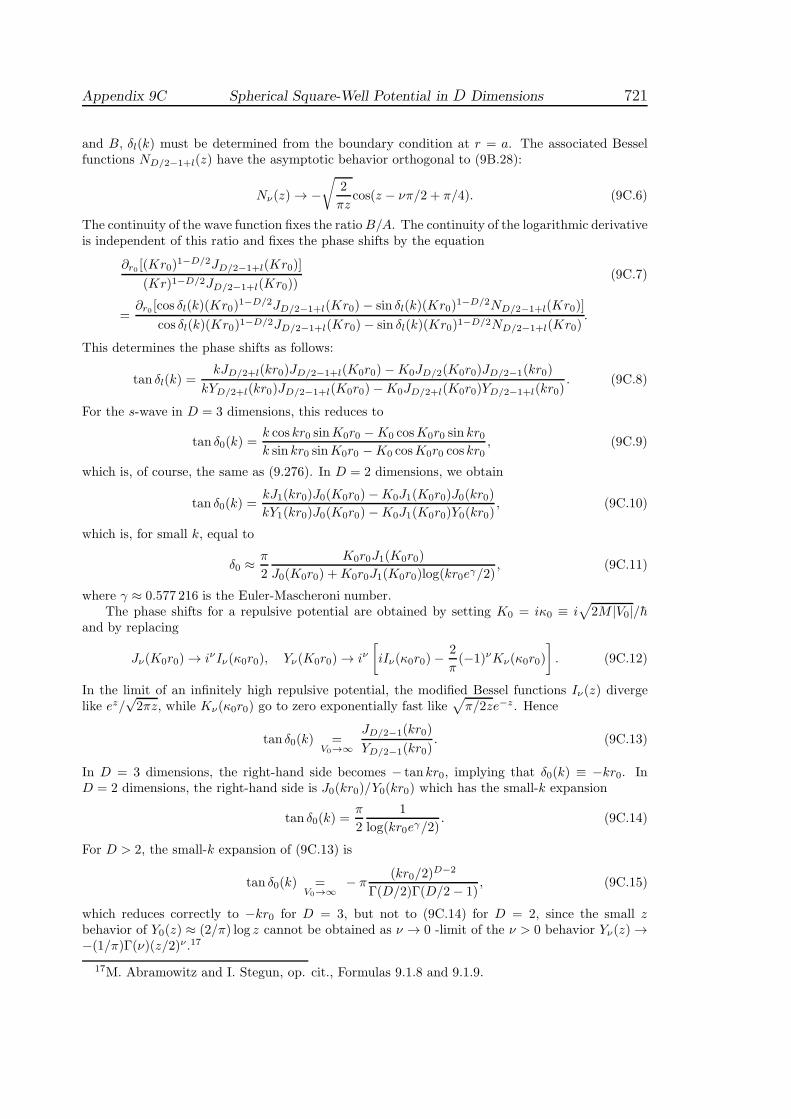
Appendix 9C Spherical Square-Well Potential in D Dimensions 721
and B, δl(k) must be determined from the boundary condition at r = a. The associated Besselfunctions ND/2−1+l(z) have the asymptotic behavior orthogonal to (9B.28):
Nν(z)→ −√
2
πzcos(z − νπ/2 + π/4). (9C.6)
The continuity of the wave function fixes the ratioB/A. The continuity of the logarithmic derivativeis independent of this ratio and fixes the phase shifts by the equation
∂r0 [(Kr0)1−D/2JD/2−1+l(Kr0)]
(Kr)1−D/2JD/2−1+l(Kr0))(9C.7)
=∂r0 [cos δl(k)(Kr0)
1−D/2JD/2−1+l(Kr0)− sin δl(k)(Kr0)1−D/2ND/2−1+l(Kr0)]
cos δl(k)(Kr0)1−D/2JD/2−1+l(Kr0)− sin δl(k)(Kr0)1−D/2ND/2−1+l(Kr0).
This determines the phase shifts as follows:
tan δl(k) =kJD/2+l(kr0)JD/2−1+l(K0r0)−K0JD/2(K0r0)JD/2−1(kr0)
kYD/2+l(kr0)JD/2−1+l(K0r0)−K0JD/2+l(K0r0)YD/2−1+l(kr0). (9C.8)
For the s-wave in D = 3 dimensions, this reduces to
tan δ0(k) =k cos kr0 sinK0r0 −K0 cosK0r0 sin kr0k sin kr0 sinK0r0 −K0 cosK0r0 cos kr0
, (9C.9)
which is, of course, the same as (9.276). In D = 2 dimensions, we obtain
tan δ0(k) =kJ1(kr0)J0(K0r0)−K0J1(K0r0)J0(kr0)
kY1(kr0)J0(K0r0)−K0J1(K0r0)Y0(kr0), (9C.10)
which is, for small k, equal to
δ0 ≈π
2
K0r0J1(K0r0)
J0(K0r0) +K0r0J1(K0r0)log(kr0eγ/2), (9C.11)
where γ ≈ 0.577 216 is the Euler-Mascheroni number.The phase shifts for a repulsive potential are obtained by setting K0 = iκ0 ≡ i
√
2M |V0|/hand by replacing
Jν(K0r0)→ iνIν(κ0r0), Yν(K0r0)→ iν[
iIν(κ0r0)−2
π(−1)νKν(κ0r0)
]
. (9C.12)
In the limit of an infinitely high repulsive potential, the modified Bessel functions Iν(z) divergelike ez/
√2πz, while Kν(κ0r0) go to zero exponentially fast like
√
π/2ze−z. Hence
tan δ0(k) =V0→∞
JD/2−1(kr0)
YD/2−1(kr0). (9C.13)
In D = 3 dimensions, the right-hand side becomes − tankr0, implying that δ0(k) ≡ −kr0. InD = 2 dimensions, the right-hand side is J0(kr0)/Y0(kr0) which has the small-k expansion
tan δ0(k) =π
2
1
log(kr0eγ/2). (9C.14)
For D > 2, the small-k expansion of (9C.13) is
tan δ0(k) =V0→∞
− π (kr0/2)D−2
Γ(D/2)Γ(D/2− 1), (9C.15)
which reduces correctly to −kr0 for D = 3, but not to (9C.14) for D = 2, since the small zbehavior of Y0(z) ≈ (2/π) log z cannot be obtained as ν → 0 -limit of the ν > 0 behavior Yν(z)→−(1/π)Γ(ν)(z/2)ν.17
17M. Abramowitz and I. Stegun, op. cit., Formulas 9.1.8 and 9.1.9.

722 9 Scattering and Decay of Particles
Notes and References
For more details on scattering theory seeS. Schweber, Relativistic Quantum Fields , Harper and Row, N.Y., 1961.
The individual citations refer to:
[1] See Chapter 3 inM.L. Goldberger and K.N. Watson, Collision Theory, John Wiley and sons, New York 1964.
[2] The unique extension of the linear space of distributions to a semigroup that includes alsotheir products is developed in the textbookH. Kleinert, Path Integrals in Quantum Mechanics, Statistics, Polymer Physics, and Finan-
cial Markets, World Scientific, Singapore 2009 (http://klnrt.de/b5).
[3] J.M.J. Van Leeuwen and A.S. Reiner, Physica 27, 99 (1961));S.A. Morgan, M.D. Lee, and K. Burnett, Phys. Rev. A 65, 022706 (2002).
[4] N. Levinson, Dansk. Videnskab. Selskab Mat.-fys. Medd. 25, Np. 9 (1949).
[5] G. Takeda, Phys. Rev. 101, 1547 (1956).