Scattering of rayleigh lamb waves from a 2d-cavity in an elastic plate

WAVE MOTION 6 (1984) 205-222 NORTH-HOLLAND

205

SCATTERING OF RAYLEIGH LAMB WAVES FROM A 2d-CAVITY IN AN ELASTIC PLATE

Anders KARLSSON Institute of Theoretical Physics, S-412 96 Giiteborg, Sweden

Received 21 December 1982, Revised 1 June 1983

The T-matrix method is applied to the problem of scattering of Rayleigh-Lamb modes from a twodimensional cavity in an elastic plate. A formal solution is obtained which is valid also for non-planar surfaces. Explicit expressions and numerical results are given for a plate with plane surfaces.

1. Introduction

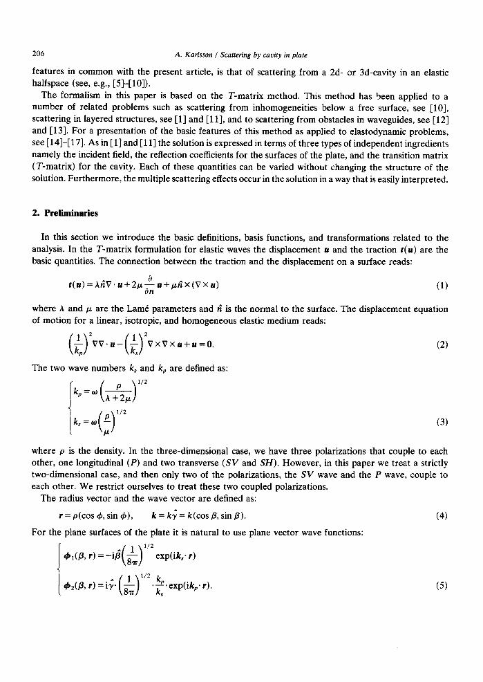
In an elastic plate with plane surfaces two sorts of guided modes exist, the SH wave modes and the Rayleigh-Lamb modes. The former modes are analogous to acoustic modes in a two-dimensional acoustic waveguide. The latter modes are of a more complex nature since they consist of coupled SV and P waves. There exist two types of Rayleigh-Lamb modes, the symmetric and the antisymmetric modes. In Fig. 1 the displacement of the plate during these modes is illustrated. In the present article we restrict ourselves to scattering of Rayleigh-Lamb modes. The corresponding problem for SH waves can be seen as a special case either of the formalism in this paper or of the problem treated in [ 11, i.e. scattering of acoustic waves from inhomogeneities in layered structures.

Scattering and responses from cavities in elastic solids are of great interest, e.g., in nondestructive testing, and a number of articles have treated this subject. However, there seem to be no articles written

on the title problem. Related problems concerning responses from centrally placed cracks in a plate have been studied in [2]-[4] using Laplace and Fourier transforms. Another related problem which has several

Fig. 1. The displacement of the plate during a symmetric mode (a) and an antisymmetric mode (b).

0165-2125/84/$3,00 @ 1984, Elsevier Science Publishers B.V. (North-Holland)

206 A. Karlsson / Scattering by cavity in plate

features in common with the present article, is that of scattering from a 2d- or 3d-cavity in an elastic halfspace (see, e.g., [SHlO]).

The formalism in this paper is based on the T-matrix method. This method has been applied to a number of related problems such as scattering from inhomogeneities below a free surface, see [lo], scattering in layered structures, see [l] and [ll], and to scattering from obstacles in waveguides, see [12] and [13]. For a presentation of the basic features of this method as applied to elastodynamic problems, see [ 14]-[ 171. As in [l] and [ 1 l] the solution is expressed in terms of three types of independent ingredients namely the incident field, the reflection coefficients for the surfaces of the plate, and the transition matrix (T-matrix) for the cavity. Each of these quantities can be varied without changing the structure of the solution. Furthermore, the multiple scattering effects occur in the solution in a way that is easily interpreted.

2. Preliminaries

In this section we introduce the basic definitions, basis functions, and transformations related to the analysis. In the T-matrix formulation for elastic waves the displacement u and the traction I(U) are the basic quantities. The connection between the traction and the displacement on a surface reads:

t(U)=hAV.u+2~~u+~riX(VXu) (1)

where A and p are the Lame parameters and ri is the normal to the surface. The displacement equation of motion for a linear, isotropic, and homogeneous elastic medium reads:

The two wave numbers k, and k,, are defined as:

l/2

(2)

(3)

where p is the density. In the three-dimensional case, we have three polarizations that couple to each other, one longitudinal (P) and two transverse (SV and SH). However, in this paper we treat a strictly two-dimensional case, and then only two of the polarizations, the SV wave and the P wave, couple to each other. We restrict ourselves to treat these two coupled polarizations.

The radius vector and the wave vector are defined as:

r = p(cos f#+ sin c#J), k = kq = k(cos /3, sin p). (4)

For the plane surfaces of the plate it is natural to use plane vector wave functions:

(5)

A. Karlsson / Scattering by cavity in plate 207

We also introduce the notation q5j for the corresponding wave functions with all i’s changed to -i. For the cavity, on the other hand, it is more convenient to use cylindrical vector wave functions:

where E” = 2 - SO,“, and cr=e, o (even, odd). The corresponding regular wave functions with Bessel ,_~ functions J,( kp) instead of Hankel functions H’,” (kp) will be denoted Re xIUn (r). The regular wave functions do not constitute a complete set at the inner resonances. However, numerical experiences indicate that one has to hit an eigenvalue with typically an accuracy of six or more digits in order to get numerical instability. In the numerical examples we consider cavities in shape of elliptic cylinders and for these the set Re x seems to be the best choice. For a discussion of the completeness of plane and cylindrical wave functions on a plane and a cylinder, respectively, we refer to [ 181 and [19].

In the analysis the transformations between cylindrical and plane basis functions are essential. These transformations are, see, e.g., [20]:

(7)

where k is the multiindex (7, a, n). The transformation functions are defined as:

(9)

The integration contours C+ and C_ are given in Fig. 2. The C+ and C_ contours can be deformed in the

ReD .

Fig. 2. The integration contours C+ and C_.


region marked with lines. Based on Eq. (2) we introduce the Green’s dyadic, e, normalized according to:

( > 2

$ vv’G(r,r’)- ; 0

2

P s

vxvxb(r,rl)+b(r,rl)=-~S(r-rl), s

(11)

where fis the unit dyadic. From this Green’s dyadic we construct the Green’s surface traction dyadic, as:

n^* 2 (r, r’) = t(&r, r’)). (12)

Where the traction operator t acts on r. The expansions of the Green’s dyadic in plane and cylindrical basis functions read:

G( r, r’) = 2i dP{+j(P, r)+f (P, r)); Y s Y’, (13) c*

&c r’) = i; Re xdr<)xk(r>) (14)

where r,(r,) denotes the radius vector with the greatest (smallest) value of p and p’. By inserting these expansions in Eq. (12) we obtain the expansions of the Green’s surface traction dyadic:

dP{r(4j(P, r))+j(p, r’)); Y 2 Y’, (15)

i C f(Re x&))xk(r’); P <P’ (16)

t(Xk(r)) Re Xk(r'); P > P’

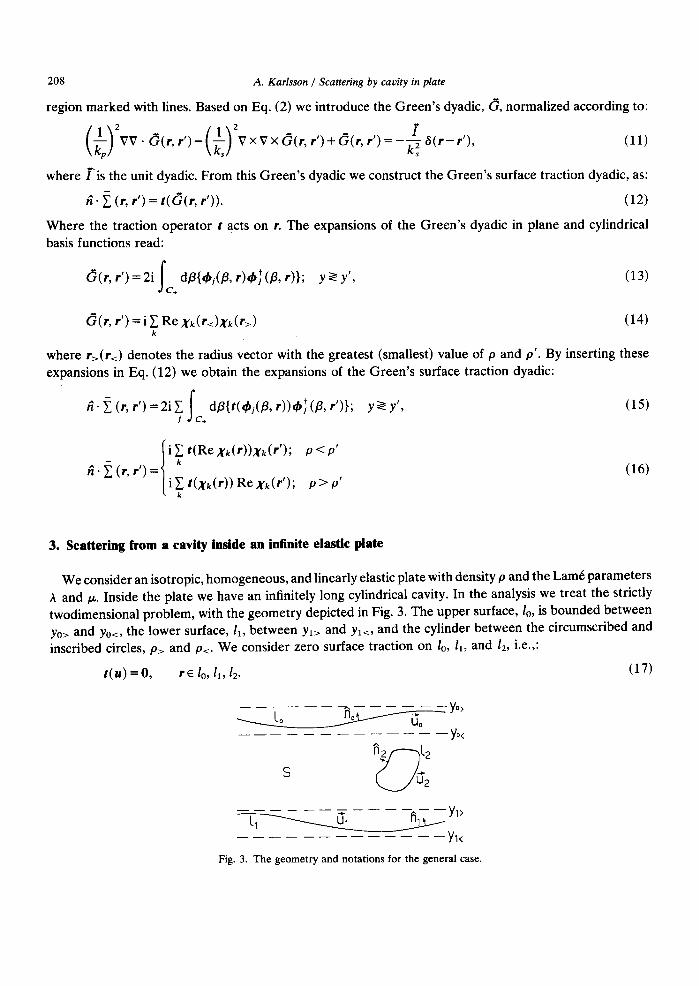
3. Scattering from a cavity inside an infinite elastic plate

We consider an isotropic, homogeneous, and linearly elastic plate with density p and the Lame parameters A and CL. Inside the plate we have an infinitely long cylindrical cavity. In the analysis we treat the strictly twodimensional problem, with the geometry depicted in Fig. 3. The upper surface, lo, is bounded between yo, and yo<, the lower surface, Ii, between yl, and yl<, and the cylinder between the circumscribed and

inscribed circles, p, and p<. We consider zero surface traction on lo, 1i, and 12, i.e.,:

r(u)=O, r E lo, 11912. (17)

S

___------ -- - - Yl<

Fig. 3. The geometry and notations for the general case.


The starting point for the formalism is the general integral formula for the displacement field, see, e.g., [16]. Under suitable radiation conditions we obtain:

uo(r’) - (&,e 2 (r, r’)) dlb +& I

ui(r’) - (A1 * f (I: r’)) dl; P 11

u2(r’) - (f&m 2 (rlr’)) dl;

{

u(r); rES = 0; WS.

(18)

Here uinc is the field from the source in an unbounded isotropic elastic space. In the integral representation we have taken the boundary conditions into account. We expand the surface displacements on lo and I1 in plane waves, and on l2 in regular cylindrical waves:

+Ar) = 1 I

dP aj(P)4j(P, r), (19) i C+

4(r) = 2 J d@ Kj(P>+j(P, 4, i c_

(20)

(21) k

The choice of expansions here is not unique. For instance, either of the C+ and C_ contours can be used in the plane wave expansions. The incident field is expanded in the following way:

~‘“S(r)=~akReXkw; P<P<, (22)

uinc( r) = C I @ aj(P)4ji(P, r); Y g YPP i C,

(23)

where the source is located at a point rp These representations of the incident field are quite general and most sources can be represented in this way.

In order to facilitate the presentation of the formal derivation of the solution we introduce an abbreviated notation, originally introduced in [l] and [ll]. Thus we adopt the notations:

(24)

i.e. the argument p is represented by an arrow, whose direction indicates the domain of definition of p according to Eq. (24). Integration over p and summation over j are indicated in the following way:

I? J dPfi(P)gj(P) =.frgr (25) i-1 C+

and similarly figr for C_ integration Summation over the indices n and 7 is suppressed as:

; && = A&. (26)

Notice that k is a multiindex (7, a, n) (cf. the remark after Eq. (9)). As an illustration, the Eqs. (13) and


(23) read in this abbreviated notation:

&r,r’)=2i {

9+)&r’); Y > Y’

+i(rMi(r’); Y <Y’,

Uinc( r) =

t

v#q(r); Y > Y,

44ltr); Y <yp

(27)

(28)

In Eqs. (19)-(21) we have three unknown expansion coefficients. Thus we need three independent equations, and these are obtained from the integral formula Eq. (18), by considering in turn

(1) an r inside the inscribed circle of 1,;

(2) a y>Y0>,

(3) a Y<YI<,

Furthermore, we insert the appropriate expansions of the incident field, Eqs. (22) and (23), the expansions of the surface fields, Eqs. (19)-(21), and the expansions of the Green’s surface traction dyadic, Eqs. (15) and (16). Eventually the three equations read:

Rexk(r)ak=i(~l(r)Q~t’Yt-~t(r)Q~SKI-Rexktr)Qkk,(Yk,), (29)

&(r)a, =i(~,(r)Q~t~r-9l(r)QflK1-xk(r) Re Qw~v), (30)

+r(r)al =i(4l(r)Q&at- br(r)Q&J-x&) Re Qww). (31)

Here we have introduced the matrix Q for the cavity:

QW =: I

Re xdr’) * t(xk(r’))dl;, I 2

(in Re QkkO, t(,yk) is replaced by t(Re xk)), and the Q-functions:

(32)

(33)

(and similarly for Qy&, Q+J, and Q;?).

In the next step we apply the transformations between the plane and cylindrical waves. Thus we insert Eq. (7) in Eqs. (30) and (31), Eq. (9) in Eq. (29), and make use of the linear independence of the plane

and cylindrical waves in a half plane and a circle, respectively. The system of equations (29)-( 3 1)) then reads:

at = i(Q& - Q;JKL) - 2DtkT~c~, (34)

a~ = i(Qy+r - Q~JKJ) -~&Twcv, (35)

ak= i(Dt,lQ~,a,-DtktQ~lK1)+ ck7 (36)

where T/&s, i.e. the T-matrix for the cavity, and the vector ck are defined as:

Tkk’ = -Re Q,,,*Q;&, (37)

ck = -iQkk’(rk’. (38)

The system of equations (34)-(36), may now be solved in a formal way if we introduce the inverses of the Q-functions. Before we solve it, we identify the operators which are generalizations of the reflection

A. Karlsson / Scattering by cavity in plate

coefficients for a plane interface:

R& =-Q:TM2;t)-1,

Rir = -Q;3_(Q:J1.

The coefficients at and K~ are now :obtained as:

at = -i(Q&)-‘(1 -R~JRT~>-’

(~~+RF~a~+2(0~k+Rf1D~k)Tkk,~k,},

K~ = i(Q~L)-l{l - R~rR~~}-‘{a~+ R~p-q+2(0~~ +R~~D~~)~wCv~.

The vector ck is implicitly given by the matrix equation:

ck = dk + Rkk’Tk’k”Ck”

where the vector dk is given by:

dk = ak +~:~R~~{l-R~~R~r}-1{U~+R~~U,}+~tkrR~,{l-R~lR~t}-1{U~+R~lUl}

and the matrix Rkko by:

R/& =2&R;,(l -R~,Rf,}-‘{~~,,+R’1,~,,.}+2~t,,RO,,{I -R’,,RO,,}-‘{D,,,+R’,,D,,,}.

211

(39)

(40)

(41)

(42)

(43)

(44)

(45)

Finally, we obtain the displacement field by considering an r inside S in Eq. (18). We separate the field in two parts:

U(f) = P’(r)+ UBnom(r) (46)

where udir is the field without any inhomogeneity present, and uanom is the field which reflects the presence

of the inhomogeneity. The explicit expressions are:

udir(r) = uinc(r) + &Jr)R&{l - RfLR&}-l{a,+ R;lal}

+~T(r)R~~{l-R~~Rf~}-‘{U~+R~rUt} (47)

and

Uanom(f)=2~1(r)RO~{1-R:~R~r}-1{D~k+R~fD~k}Tkk,Ck,

+2~,(r)R,‘,{l-R~,R,‘,}-‘{D,,+R~,D,k}Tkk,ck,

+Xk(d Tkk’ck’ (48)

4. Specialization to a plate with plane surfaces

When the surfaces lo and l1 are plane, the Q-functions may be calculated explicitly due to the orthogonality of the plane wave basis functions on a plane surface. If we insert the calculated expressions for the Q-functions and their inverses in Eqs. (39) and (40), we will get the wellknown reflection coefficients for elastic waves at a plane surface times a delta function which expresses Snell’s law for elastic waves:

RYt = R$gjr(Pj, By), (49)

RTll = R;rgj&, &), (50)


where g&Q, &) is the distribution:

gjf(pj, pjf) = djj’S(pf +pj) + 8j,18f,2S pf +arccos k + Sj,*Sj JS pjf +arccos t { ( :I ’ ( J* (51)

We have introduced an index on the p-variable due to the coupling between SV and P waves from Snell’s law. The reflection coefficients in Eqs. (49) and (50) read:

C RY =4q2h,h,-(hf-qZ)*

II A {~j,1%,0 exp(2ihd + &&,o exp(2ih,yd + 6j,lSv,1 exp(-2iha)

;t- aj,z&,I exp(-2ihPyI)I

RY =4q(h: -q*) II’ A

{(hp&+,t - h&&,d&,o exp[i(h, + h,)yol

L +(h~~j,~~~,2_hp~j,2~~,~)Sv,~ exp[-i(h,+ hp)yd. (52)

We have introduced the notations:

{

q = ki COS( pi)

hi=(kf-q2)1’2, i=l,2(s,p), (53)

i.e. the wavenumbers in the x-direction and the positive y-direction, and:

A = 4q2h,hP + (hf - q2)2. (54)

The Rayleigh poles are then given by the equation:

A=0 (55)

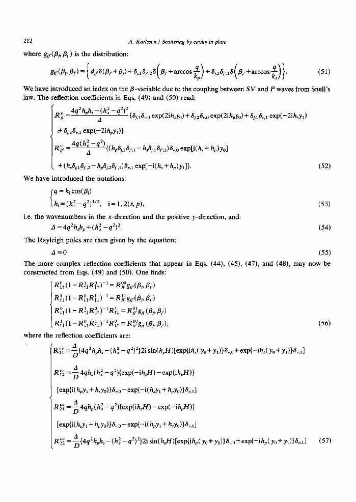
The more complex reflection coefficients that appear in Eqs. (44), (45), (47), and (48), may now be constructed from Eqs. (49) and (50). One finds:

1

R~t.(l-RF~R~,)-‘=R~gj~(Pj,Pj’)

~;&(l-~~,~fd -l = qj?gjj,(pj, pi,)

R&(l-R~~R&-‘Rf~ =Ri’gjf(Pj,Pf)

RiJ (1 - Ry,RiL)-‘Rf, = RiFgjj,(Pj, pi,), (56)

where the reflection coefficients are:

R;; = ${4q2hPh, -(h: - q2)2}2’ 1 sin(h$f)[ewM yo+ ydb%o+expI-iM YO+ YI)R,II

R ;g = $4qh,( hz - q2){exp(-iha) - exp(ihfl)}

[expIi(h,y, + h,y,)}6,,-exp(-i(h,yl+ h,yo)bU ‘

RGy =$4qh,(hf -q2){exp(ihfl)-exp(-ih$)}

[exp(i(h,y, + h,yo)}S,o-exp(-i(h,y, + hsyd&l

R;; =${4q2hPh,-(h: -q2)2}2isin(h~)[exp(ih,(yo+yl)~S,o+expI-ih,(y~+y~)~~,~1 (57) I

A. Karlsson 1 Scattering by cavity in plate 213

I

R”’ CR;: = 11 exp(Ea) [2i sin(h$)A*+{exp(-ih$) -exp(-ihfi)}16q*h,h,(~~ -q2)2]

Ry: =[ex~i(h~-h,)y~}-ex~i(h~-h~)Y0}]~4q2h h _(h2 _q2)2}4qh D PS s

(h2 _q2) s s

RX: = expMh,- h,)tyo+ yJ)R%? s

<

Rt! Jexp{ith,- h~)yl~-exp~ith,-h~)y~~l14q2h D

h _th2 _q2)2j4qh

PS s

th2 _q2) s s

JGY =expIi(h.-h,)(yo+yl)}R~~~ s

Ro’ 22

=R’o = 22 -[2i sin(hfi)A*+{exp(-iha)-exp(-ih$)}16q2h,hp(h~ -q*)*],

where H = yo- y,. The denominator D is defined as:

(h: -q*)* sin(y) c,(y) +4q2hph, sin(y) cos(y)}.

(58)

(59)

We then obtain the Rayleigh-Lamb equations from the mode equation, D = 0, i.e.: .

tan( h,H/ 2) Ih: -q*)* tan( h,H/2) = - 4q2hphs

(f-50)

for antisymmetric modes, and:

a= _V+q*)*

tan(kJJ/2) Q*hphs (61)

for symmetric modes (cf. Fig. 1). The Rayleigh-Lamb equations have been treated thoroughly in the literature, see, e.g., [21] and [22]. The expressions for the reflection coefficients are now inserted in Eqs. (44), (45), (47), and (48). The integrals in these equations may be calculated by numerical integration. However, in most cases it is convenient to express the vector dk, the direct field, and the anomalous field as mode sums. The criteria for when these mode sums are favourable numerically are discussed in Section 5. From Eqs. (22), (23), and (9) we have:

ak = D&a, = DLlar (62)

We insert the right hand side of Eq. (62) (either the C+ integral or the C_ integral) in Eq. (44) and combine it with the original C+ and C_ integrals. After some rearrangements we eventually obtain:

dk=&-I,) dpjDt,(~j){Ej~(Pj)aj,(-B~)+~~(Pj)a~(Bf)}. (63)

The direct field and the anomalous field are rearranged in an analogous manner. If we insert Eq. (23) in


Eq. (47) and Eq. (7) in Eq. (48) we obtain the following expressions:

where:

qj’@j) = {

R$(q, hm hp); PjE C+ Ri’(q,-hs,-hp); PjE C-’

The argument /37 is related to @j according to (cf. Eq. (51)):

Pj; j= j'

pf = arccos 4 0 - ; k

j=2,j’=l

(66)

(67)

1 0 4 arccos - ;

kP

j=l,f=*

The C+ and C_ contour may now be closed in Eqs. (63)-(65). We have branchpoints at cos(&) = k,/ k,

in the Pi-plane and at cos(&) = k,/k, in the &-plane, we thus have to examine which Riemann surfaces the contours C+ and C_ and the physical poles belong to. The C+ is considered for upward traveling waves and C_ for downward traveling waves (cf., e.g., Eq. (7)). Thus the imaginary part of both sin&) and sin(&) are nonnegative on the C+ contour and nonpositive on the C_ contour. Furthermore, a criterion for a physical pole is that the imaginary parts of sin(&) and sin(&) have the same sign. The statements above define how the C+ and C_ integrals in Eqs. (63)-(65) are to be closed. In Fig. 4 the closed integration paths C’ and C”, the cuts, and the poles in the &-plane are illustrated. As seen from the integrands in Eqs. (63)-(65), we have to shift the C_ contour 27r in the negative Re pi direction when xP < 0 in Eq. (63), x > x,, in Eq. (64), and x > 0 in Eq. (65), in order to obtain the closed contour C’. Otherwise, i.e. for waves propagating in the negative x-direction, the contour C” is considered. The conclusion is that the closed contour follows the Riemann surface where the imaginary parts of siri and sin(&) have the same sign. For waves propagating in the positive (negative) x-direction the C’(C) contour is obtained. The nonpropagating modes are then exponentially decaying. According to Eqs. (60) and (61) there are infinitely many poles to take care of (but only a finite number of them corresponds to propagating modes). In Fig. 4 we have only indicated six poles, though the C’ and C” contours are understood to take care of all physical poles. The six poles in Fig. 4 correspond to two propagating modes (those with real cos(pi)) and one nonpropagating mode (with imaginary cos(&)).

It is illustrative to give the explicit expressions for the mode sums. Up to this point we have had essentially no restrictions on the source, but now we specialize it to be a point force, normalized according to:

ak =iB* ~k(rJ

Ut=Uj(P)=*i~‘~j(p,rp); PEC+

lU(=Uj(B)=2i~.9j(P,rp); PeC_ (68)


i--

I

C'

,\: -tt

mlk ____--

Fig. 4. The integration contours C’ and C” with cuts (-) and poles (X). The branchpoints are at cos p1 = k,/ k, The contours follow the Riemann surface where the imaginary parts of sin /S1 and sin & have equal signs. The cuts are chosen SO that sin p1 and sin &

are real along the cuts.

where $ is the direction of the point force:

B = (cos(rl), sin(q)). (6%

It is convenient to separate the mode sum in one antisymmetric and one symmetric part. If, for simplicity, we consider the source to be a symmetrically located point force, i.e. yP = ( yO+ yJ/2, the explicit expression for the vector dk reads:

dk = *(HIT)“‘; [

sin( 7) C $$ exp(-iqx,) (

1 + (h5 - q2) cos( h,H/2)

S a 2q2 cos(hPl2) >

{ m <@k tPT)exp(-i&y,)

+@k (-PT) exp(W,)) - (‘,!j~q2)(& <Pb )exp(-ih,y,) - DL (-8f)exp&yJ)} P

-cod 17 ) 1 q’h:h,

s f(4) exp( -iqx,)

( l-

(hz -4’) sin(h&/2)

2 h,h, sin( h&l/ 2) )I

sir, (h&f/2)

sin( hJ3/2)

<& (BT) ev(-i&J - % (-PT) exp(ih,y,))

-$$$(&.(P:) exp(--ih,y,)+%(--BT) exp(ihPyP))}]; {zz:


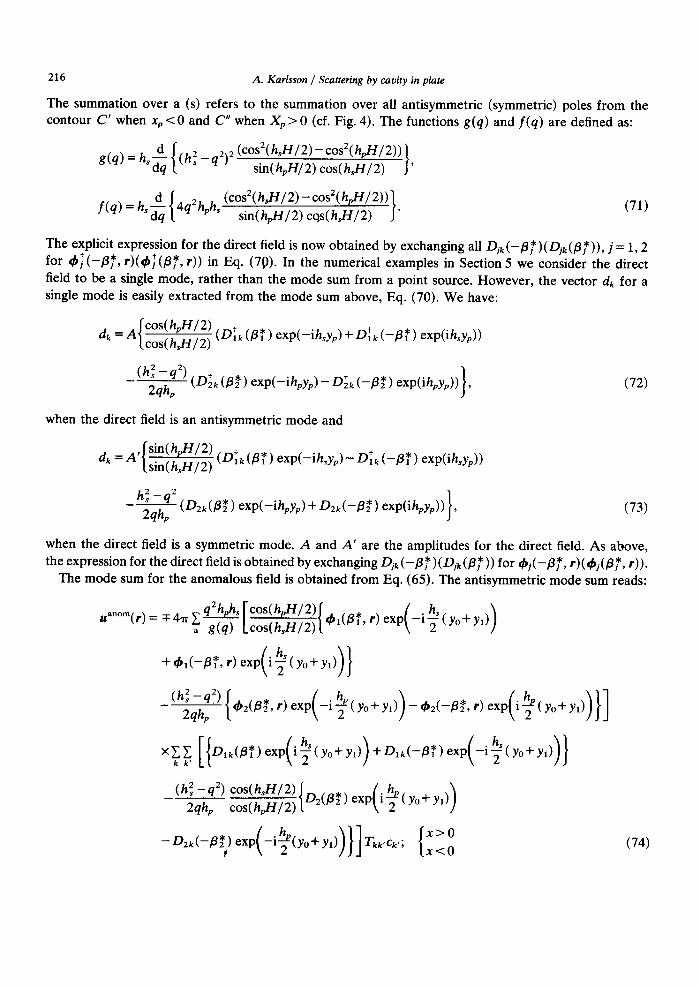
The summation over a (s) refers to the summation over all antisymmetric (symmetric) poles from the contour C’ when xP < 0 and C” when X, > 0 (cf. Fig. 4). The functions g(q) and f(q) are defined as:

&Y(q) = h,$ 02 -q212 { (cos2(hfi/2) -cos2(h$z/2))

sin( h#/2) cos( hfi/2) I ’

04) = hi 1

4q2&.k (COS2(h~/2)-cos2(hpH/2))

sin(h#/2) cqs(hJ9/2) I ’ (71)

The explicit expression for the direct field is now obtained by exchanging all Djk(-PT)(Dik(pT)), j= 1,2 for 4J(-BT, r)(4f(@, r)) in Eq. (70). In the numerical examples in Section 5 we field to be a single mode, rather than the mode sum from a point source. However, single mode is easily extracted from the mode sum above, Eq. (70). We have:

consider the direct the vector dk for a

dk = A costhd_1/2) cos(hfi,2) (o:k (PT) exp(-iky,) + D:,k (-PT) exp(ih,y,))

-(‘jGq2) (ok (Pt ) exp(--ih,y,) -I& (-p2*) exp(i&y,))}, P

when the direct field is an antisymmetric mode and

dk = A, sinthp/2) sin(ha/2) (@k(K) exp(-iky,)--&(-KY exp(ih,y,))

-!$$ (D2kUG) exp(--ihpyp)+D2k(-j3;) exp(ih,y,)) ,

P

(72)

(73)

when the direct field is a symmetric mode. A and A’ are the amplitudes for the direct field. As above, the expression for the direct field is obtained by exchanging Djk(-Pr)(Djk(PT)) for +j(-PT, r)(+j(pT, r)).

The mode sum for the anomalous field is obtained from Eq. (65). The antisymmetric mode sum reads:

Uanom( r) = r 4Tr 1 a >

+A(-PT,r) exp

- th~~hq” P 1 42@2*,r)exp -i+Ch+y,) ( > -42t-PZ,r)exp i~tyo+y,) ( 111

xcc [I DlktPT) exp k k’ (

i:( yo+ y,) +&A-PT) exp ) (

-i+(y0+yA )I

_M -q2) codWl2)

QhP

cos~hfl,2~{~2(B:) ew(i+(y0+yb)

-o,k(-/%,) exp (

-$$yO+yl) )}]Tkk,ck*; (:=,” (74)


and the symmetric mode sum reads:

Uanom( r) = =f 4lr 1 q*h,,h, sin(hfl/2)

S f(q) [ sin(hJfl2)

X 1

&(PT,r)exp -i$(y,fyJ ( >

-&(-PT,r)exp i+(Y0+Yr) (

_(h: -q*)

2& { 42033,r) exp( -i$%0+ yl)) + +2(-P2*, 4 exp( i$b+ y’))}]

Xi?l; [{

&ABT) exp i+(h+h) ( )

-&J-PT) exp -i+ty0+ yd ( )I

_ (hz -q*) sin(hSI/2)

2qh, sin( h&I/2)

X I

D2k(pq) exp (

i& 2 (Yo+Y1) >

+D2k(-P2*) exp (75)

5. Numerical examples

In this section we discuss the numerical procedure and some numerical results of scattering of Rayleigh- Lamb modes from elliptic cylindrical cavities in a free plate with plane surfaces. We consider the direct field to consist of a single mode. This is no essential restriction since sources which do not lievery close to the cavity are well approximated by a finite mode sum. In the numerical examples we illustrate either the energy reflection/transmission coefficients or the displacement field for y = yO. The energy reflection (transmission) coefficient R,( Tj) for a mode i, is defined as the ratio between the reflected (transmitted) energy flux for the mode and the energy flux for the incident mode j The energy flux is (see e.g. [15]):

P=zIm t(u) - u dy .

A necessary condition for the scattering data is:

l=C(Rij+T,i)

(76)

(77)

and this condition is fulfilled to at least five digits in the numerical examples. However, it does not imply that each Rij and Tij separately are accurate to five digits.

In order to calculate the mode sums we have to solve the mode equations (60) and (61). This is done numerically with some iterative method, e.g., the secant method. The lowest symmetric mode and antisymmetric mode exist for all frequencies of a given plate thickness. These modes become Rayleigh modes as k& goes to infinity. The cut off frequencies of the higher modes are:

k$z=(2n-l)m; n=1,2,...

k$I=2nr; n=l,2,... (78)


for antisymmetric modes, which we denote a,, and:

kfl= 2nr ;n=l,2,...

k$=(2n-l)p ;n=1,2,... (79)

for symmetric modes, which we denote s,. As we pointed out in Section 4, the vector dk, the direct field, and the anomalous field can in most cases be represented by a mode sum. However, the matrix R, Eq. (45), cannot be represented by a converging mode sum, and therefore we calculate it by numerical integration. If we integrate over the variable t = cos p,, or t = cos p2, we have to choose an integration path that avoids the poles on the real t-axis. In the numerical examples we have integrated along the line 2(2-i), z E (0, co), i.e. in the fourth quadrant. When the displacement field is calculated at a distance of less than approximately one wavelength from the cavity in the x-direction, the mode sum becomes slowly convergent and it is more favourable to calculate the anomalous field by numerical integration. This is done by integration along a path in the fourth quadrant that avoids the poles on the real axis. However, as seen from the explicit expression of the integrand, the integration path has to coincide with the real axis for large t =cos p, otherwise the integral fails to converge. We choose to integrate along the path:

cos(p) = z(1 -iaePb’); 2 E (0, co), (80)

where the constants a and b are adjusted to give best convergence. The geometry for the numerical examples is depicted in Fig. 5. The plate is considered to be an aluminium

plate with cP/cs = 642/304, and with thickness H. The cavity is an elliptic cylinder with major half axis of length a and minor half axis of length b and with its center in origo. Scattering from elliptic cylinders has been treated in [17], where the expression for the T-matrix is given. The cylinder can be rotated an angle +, which denotes the angle between the major axis and the positive x-axis. As seen from Eqs. (78) and (79) we have the following cut offs for the first modes in an aluminium plate:

mode: a0 so 4

k,H= - - 3.14 6.2s: s2 a2 s3

6.63 9.42 12.57

-- yl J / --

Fig. 5. The geometry and notations for the numerical examples.


Fig. 6. The energy reflection (a) and transmission (b) coefficients for the three modes - - - s,,; - a,,; - - - a1 ; in an aluminium plate (c,/c. = 642/304). The direct field is an s, mode. The half axes are a = H/2 and b = a/5, the plate thickness is kJ-f =4, and

the upper surface is y,, = H/2.

The first example, Fig. 6(a) and (b), shows the energy reflection and transmission coefficients for the three propagating modes, so, Q, and al, when an incident so mode is scattered from an elliptic cylinder with half axes k, a = 2 and k, b = 0.4 in a plate of thickness k, H = 4 and with k, y, = 2. The cylinder is rotated from + = 0” to 90”. We may notice that the coupling between the symmetric and antisymmetric modes is zero for I& = 0” and 90”, as expected, and has a maximum around 45”. A necessary condition is that the reflection coefficient for the so mode is one for $ = 90”, and this is fulfilled to four digits.

In Fig. 7 the energy reflection coefficient is plotted against frequency. The cylinder is symmetrically placed, i.e. y. = H/2, the half axes are a = 0.9 y. and b = a/6, and $ = 0” and 90”. The frequency interval is k, H E (0,5), and the direct field is an so mode. Since the geometry is symmetric around y = 0 the so mode does not couple to any other propagating mode in the actual frequency interval. For $ = 90” the reflection coefficient is monotonically increasing from zero to unity in the interval k,Hc (0,4.6), and then a resonance phenomenon occurs and the cavity becomes invisible, i.e. we have total transmission. When + = 0” the energy reflection coefficient is a more violent function of frequency, and several resonance phenomena occur.

In Fig. 8 we consider a centrally placed circular cylinder. The geometry then only have two free parameters. The incident mode is an so mode and kJ3 = 3. The energy reflection coefficient is plotted as a function of the radius of the cylinder. We may notice that the reflection coefficient is a complicated function of the radius of the cylinder. The behaviour of the curve in Fig. 8 is typical for a sizeable frequepcy region.

The last two figures, 9 and 10, illustrate the displacement field for three frequencies, kJY = 1, 3, and 10. The direct field in both examples is an a, mode propagating in the negative x-direction. The cylinder has major axis a = H/4 and minor axis b = u/6. In Fig. 9 y. = H/2 and the cylinder is rotated an angle + = 75”. The ratio between the anomalous and the direct field is calculated for y = y. from x = -5H to x = 5H. In Fig. 10 y. = 0.3H and $ = 90”. The ratio between the total and the direct field is calculated for y = y. in the same x-interval as above. We may notice that for kJ3 = 1 the displacement fields are only marginally disturbed by the cavities. For kfi = 5 and 10 there is more structure in the displacement field due to the increasing scattering cross section and that more propagating modes exist (3 for kJl = 5


1.c

C

I- R

k,*H

L

o/H

I

0.5

Fig. 7. The energy reflection coefficient as a function of Fig. 8. The energy reflection coefficient as a function of the frequency in an aluminium plate. The direct field is an se mode. radius of a symmetrically placed circular cylinder in an The half axes are a = 9H/20 and b = a/4, the upper surface aluminium plate. The incident mode is an su mode, and the is y0 = H/2, and the rotation angle is ----I) = 90”; - -- JI = 0”. plate thickness is kJ-I = 3.

1.0

0

t

R

-5 0 5 X/H

Fig. 9. The absolute value of the anomalous field on the upper surface, y. = H/2, of an aluminium plate. The direct field is an a, mode propagating in the negative x-direction. The half axes are a = H/4 and b = a/6, and the rotation angle is t,k = 75”. The plate

thicknessis-kfi=l;---kfi=S;---kfi=lO.

and 6 for kJY = 10). However, the disadvantage of measuring the displacement field at high frequencies is that the total field varies very rapidly with x as is seen from Fig. 10.

In the numerical examples we have demonstrated some possible applications of the method, e.g. scattering from nonsymmetrically placed cavities, rotated cavities, and cavities touching the planes. Some numerical results are unexpected, e.g. the resonance phenomenon in Figs. 7 and 8, and they illustrate the irregularities in low frequency scattering. Extensions that may be considered in future work are a 3d-formalism and an introduction of the T-matrix for a crack. We remark that the formal solution, Eqs (43)-(48), and the expressions for the reflection coefficients, Eqs (56)-(58), hold even in the 3d-case.

A. Karlsson / Scattering by caoity in plate 221

-5 0 5 X/H

Fig. 10. The absolute value of the total field on the upper surface, y. = 3 H/ 10, of an aluminium plate. The direct field is an a0 mode propagating in the negative x-direction. The half axes are a‘= H/4 and b = a/6, and the rotation angle is 9 = 90”. The plate

thicknessis---kfi=l;---kfi=5;-k,.H=lO.

Acknowledgment

The author wishes to thank Drs. A. BostrGm, G. Kristensson, and S. Striim for valuable discussions and comments during the work.

References

[l] A. Karlsson, “Scattering from inhomogeneities in layered structures”, J. Acoust. Sot. Am. 71, 1083-1092 (1982). [2] E.P. Chen, “Impact response of a finite crack in a finite strip under anti-plane shear”, Eng. Fract. Me&. 9, 719-724 (1977). [3] E.P. Chen, “Sudden appearance of a crack in a stretched finite strip”, J. Appl. Me& 45, 277-280 (1978). [4] S. Itou, “Transient response of a finite crack in a strip with stress-free edges”, J. Appl. Me&. 47, 801-805 (1980). [5] S.K. Datta and Nabil El-Akily, “Diffraction of elastic waves by a cylindrical cavity in a halfspace”, J. Acousr. Sot. Am. 64,

1692-1699 (1978). [6] S.K. Datta and Nabil El-Akily, “Diffraction of elastic waves in a half space I: Integral representations and matched asymptotic

expansions”, in: Modern Problems in Elastic Wave Propagation, Wiley, New York (1978). [7] J.H.M.T. van der Hijden, “Diffraction of elastic waves by a cylindrical crack in a semi-infinite solid (in plane motion)“, Report

no. 1981-11, Laboratory of Electromagnetic Research, Dept. of Electrical Eng., Delft University of Technology (1981). [8] J.D. Achenbach and R.J. Brind, “Scattering of surface waves by a sub-surface crack”, J. ofsoundand Vibration 76,43-56 (1981). [9] R.J. Brind and J.D. Achenbach, “Scattering of longitudinal and transverse waves by a sub-surface crack”, .J. of Sound and

Vibration 78, 555-563 (1981). [lo] A. Bostram and G. Kristensson, “ Elastic wave scattering by a three-dimensional inhomogeneity in an elastic half space”, Wave

Motion 2, 335-353 (1980). [ 111 A. Karlsson and G. Kristensson, “Electromagnetic scattering from subterranean obstacles in a stratified ground”, Radio Science

(to appear). [12] A. Bostriim, “Transmission and reflection of acoustic waves by an obstacle in a waveguide”, Wave Motion 2, 167-184 (1980). [13] A. BostrGm and P. Olsson, “Transmission and reflection of electromagnetic waves by an obstacle inside a waveguide”, J. Appl.

Phys. 52, 1187-1196 (1981). [ 141 PC. Waterman, “Matrix theory of elastic wave scattering. I”, J. Acous. Sot. Am. 60,, 567-580 (1976).


[15] P.C. Waterman, “Matrix theory of elastic wave scattering. II. A new conservation law”, .I. Acoust. Sot. Am. 63, 1320-1325 (1978).

[16] V. Varatharajulu and Y.-H. Pao, “Scattering matrix for elastic waves. I. Theory”, J. Acoust. Sot. Am. 60, 556-566 (1976). [17] V.V. Varadan, “Scattering matrix for elastic waves. II. Application to elliptic cylinders”, J. Acoust. Sot. Am 63, 1014-1024

(1978). [ 181 Cl. Kristensson, “Electromagnetic scattering from buried inhomogeneities-a general three-dimensional formalism”, J. Appl.

Phys. 51, 34863500 (1980). [19] P.A. Martin, “Acoustic scattering and radiation problems, and the null-field method”, Wave Motion 4, 391-408 (1982). [20] A. Bostrom, G. Kristensson, and S. Strom, “Transformation properties of plane, spherical, and cylindrical scalar and vector

wave functions, in: Handbook on Acoustics, Electromagnetic, and Elastic Wave Scattering, Vol. I, North-Holland, Amsterdam (1983), to appear.

[21] J. Miklowitz, The Theory of Elastic Waves and Waveguides, North-Holland, Amsterdam (1978). [22] W.M. Ewing, W. S. Jardetzky, and F. Press, Elastic Waves in Layered Media, McGraw-Hill, New York (1957).

Scattering of rayleigh lamb waves from a 2d-cavity in an elastic plate

Documents

Transcript of Scattering of rayleigh lamb waves from a 2d-cavity in an elastic plate