Wave Motion 51 (2014) 517–532

Contents lists available at ScienceDirect

Wave Motion

journal homepage: www.elsevier.com/locate/wavemoti

Scattering of a plane harmonic SH wave by multiplelayered inclusionsRamtin Sheikhhassani ∗, Marijan DravinskiDepartment of Aerospace and Mechanical Engineering, University of Southern California, Los Angeles, CA 90089, USA

h i g h l i g h t s

• Scattering of a plane harmonic SH wave by multiple layered inclusions is considered.• Boundary integral equation method is applied to solve the problem.• The effects of multiple scattering, the geometry, and the impedance contrast on surface motion are investigated.• The importance of these factors on the surface response is demonstrated.

a r t i c l e i n f o

Article history:Received 3 August 2013Received in revised form 4 November 2013Accepted 7 December 2013Available online 24 December 2013

Keywords:Wave propagationMultiple scatteringMultilayered inclusionsElastic wavesAnti-plane strainBoundary element method

a b s t r a c t

Scattering of a plane harmonic SH wave by an arbitrary number of layered inclusionsin a half-space is investigated by using a direct boundary integral equation method. Theinclusions of arbitrary shape and placement are embeddedwithin an elastic half-space. Theeffects of multiple scattering, the geometry, and the impedance contrast of the materialsfor layered inclusions and pipes are considered in detail.

© 2013 Elsevier B.V. All rights reserved.

1. Introduction

Diffraction ofwaves bymultiple scatterers has been subject of numerous investigations in the past. This problem arises inthe fields of elastodynamics, acoustics, electromagnetics, and optics. Many applications, such as non-destructive evaluationof materials [1,2], medical imaging [3,4], and seismology [5,6] incorporate these types of models.

The methods used to study these problems are either analytical or numerical [7].The earliest classical theorywas pioneered by Foldy [8]who considered a randomdistribution of isotropic point scatterers

and derived an effective wave number for scalar waves propagating through an inhomogeneousmedium. He found that thiseffective wave number differs in the presence of scatterers.

Lax [9] followed Foldy’s procedure to include anisotropic and inelastic scattering. He introduced an effective medium inwhich scattering fluctuations were embedded. The parameters were determined by averaging, similar to Foldy’s method.

Twersky [10] employed the wave series expansion method for scattering of a plane wave by an arbitrary configurationof two parallel cylinders and spheres [11] for acoustic and electromagnetic theory.

∗ Corresponding author. Tel.: +1 3104041296.E-mail addresses: sheikhha@usc.edu (R. Sheikhhassani), mdravins@usc.edu (M. Dravinski).

0165-2125/$ – see front matter© 2013 Elsevier B.V. All rights reserved.http://dx.doi.org/10.1016/j.wavemoti.2013.12.002

518 R. Sheikhhassani, M. Dravinski / Wave Motion 51 (2014) 517–532

Waterman and Truell [12] considered finite size scatterers and obtained a second-order correction to Foldy’s formula interms of the scatterer density.

Waterman [13] devised the T -matrixmethod, which expands the components of the scattered and incident fields by a setof orthonormal vectors. Subsequently, Peterson and Ström [14–17] used the T -matrix approach to determine the scatteringof multiple and multilayered objects for the acoustic and electromagnetic theory.

Thereafter, Bose andMal [18], and Varadan et al. [19] advanced themultiple scattering theory to scalarwaves in an elasticfull-space. Specifically, they described the elastic waves and the interactions between two particles.

Berryman [20], Sabina [21], Yang and Mal [22], and Kanaun [23] approximated the interaction among particles byassuming that each particle is embedded within an effective medium.

Yang andMal [22,24] implemented a method that Christensen [25] developed to evaluate the effective elastic propertiesof composite materials. They applied it to theWaterman–Truell [12] model for the scattering of randomly distributed fibersin a composite via statistical averaging.

Kanaun and Levin [26] examined the effective medium method for axial elastic shear wave propagation through fibercomposites. Wei and Huang [27] studied the dynamic effective properties of particle-reinforced composites by modelinga thin homogeneous viscoelastic interphase between the inclusion and the matrix. Biwa et al. [28] used the eigenfunctionexpansion and collocation methods with the assumed periodicity of the fiber arrangement in the direction normal to thepropagation direction for SH and subsequently for P and SV waves [29]. Ou and Lee [30] adopted the eigenfunction expansionmethod for the scattering of S and P waves by a single nano-sized coated fiber.

The derivation of analytical solutions that satisfy both the differential equations and boundary conditions is limited toonly very simple problems [31]. For more realistic problems, one must rely on numerical procedures.

In continuum mechanics, numerical techniques such as the finite difference method (FDM), the finite element method(FEM), and the boundary integral equation method (BIEM) are often used.

For unboundedmedia, the use of BIEM is greatly preferred over the other computationalmethods. In BIEM, the governingequations are represented as integral equations. The advantage is that only the boundaries are discretized [32], instead ofthe volume of the problem, which considerably reduces the size of the system of the equations, compared with FEM. Inaddition, the radiation conditions at infinity are satisfied exactly.

In solving wave propagation problems in unbounded media using FDM or FEM, artificial absorbing boundary conditionsare introduced [33] to improve the accuracy of the solution.

A number of researchers have applied boundary integral equations to the problem of wave propagation (e.g., [34–38]).Benites et al. [39,40] implemented the BIEM for the scattering of multiple cavities in a full-space and a half-space by

SH, P , and SV waves.DeSanto [41] used boundary integral approach to study an N-layered single scatterer of arbitrarily shaped surfaces

embedded in a full-space.Dravinski and Yu [42] investigated scattering of SH waves by an arbitrary number of homogeneous inclusions of general

shape and placement within an elastic half-space by using a direct boundary integral equation approach. They examinedthe effect of inclusion locations for two, three, and nine inclusion models and demonstrated the significance of multiplescattering on the peak surface amplification.

Dravinski and Sheikhhassani [43] showed the importance of layering for a single layered obstacle embedded within ahalf-space, especially for soft materials. In addition, they showed that the impedance contrast of the layers has a significantimpact on the surface motion.

The intent of this paper is to extend Dravinski and Sheikhhassani’s [43] work to include multiple layered scatterers. Thepaper is divided into five parts. Section 2 presents the statement of the problem. Section 3 considers the solution, which isformulated using integral equations. Section 4 presents the numerical results, while Section 5 provides a summary of thepresented work.

2. Problem statement

The scattering of a plane harmonic SH wave by an arbitrary number of layered inclusions completely embedded withinan elastic half-space (Fig. 1) is investigated by using the direct boundary integral equations method. Each inclusion consistsof a finite number of layers that are perfectly bonded together. The interfaces between the layers are assumed to be C (1)

continuous without any sharp corners.The geometry of the problem is described in Cartesian coordinates {|x| < ∞; 0 ≤ z < ∞} with the z-axis pointing

downward (Fig. 1). The half-space surface and the domain are denoted as S0 and D0, respectively. The outward unit normalon various surfaces is denoted by n.

The interfaces and domains for different layers are defined by considering a generic ith inclusion, 1 ≤ i ≤ N , as shown byFig. 2. From the outermost to the innermost layers the corresponding domains are denoted by Di

1 to DiLi, respectively, where

Li represents the number of layers for the inclusion. Therefore, Dij denotes the domain of the jth layer of the ith inclusion.

The corresponding layer interfaces are represented by S i1, . . . , SiLi.

All of the layers, except the innermost one, are bounded by two interfaces. The innermost layer DiLi is bounded by only

one interface, S iLi.

R. Sheikhhassani, M. Dravinski / Wave Motion 51 (2014) 517–532 519

Fig. 1. Problem model consisting of N layered inclusions with Li, i = 1 : N layers embedded within an elastic half-space.

Fig. 2. The ring limit model for domain Dij when the observation point y is located on the boundary S ij (or S

ij+1), where i = 1 : N, j = 1 : Li − 1.

2.1. Equations of motion

The steady-state SH waves are governed by the Helmholtz equation (e.g., [44])∇

2+ [k(i)

j ]2u(i)j = 0

k(i)j =

ω

β(i)j

β(i)j =

µ(i)j

ρ(i)j

i = 0, 1 to Nj = 0, 1 to Li

(1)

where u(i)j , ω, k(i)

j , β(i)j , µ

(i)j , and ρ

(i)j are the displacement field, the circular frequency, the wave number, the shear wave

speed, the shearmodulus, and the density of the domainDij, respectively. Here,D

ij; i = 0, 1, . . . ,N; j = 0, 1, . . . , Li represent

the domains of the half-space and the layers, respectively. Specifically, the superscript (i) refers to the inclusion number,and the subscript j denotes the layer number within that inclusion.

For convenience, the following notation is adopted for the domain and displacement fields in the half-space: D0 = D00

and u0 = u(0)0 . The remaining displacements are labeled u(i)

j ; i = 1 : N; j = 1 : Li.

520 R. Sheikhhassani, M. Dravinski / Wave Motion 51 (2014) 517–532

Finally, the Laplacian operator is given by

∇2

=∂2

∂x2+

∂2

∂z2. (2)

The incident wave is assumed to be of the form

uinc(x, ω) = ei[k0(x sin(γ )−z cos(γ ))−ωt]; x ∈ D0 (3)

where γ is the off-vertical angle of incidence (Fig. 1). The exponential term e−iwt and the frequency dependence will beomitted throughout.

2.2. Boundary conditions

As the incident wave strikes the inclusions, it generates the scattered wave field. Therefore, the total displacement fieldin each domain can be written as

u0 = uff+ usc

0 ; x ∈ D0

u(i)j = usc(i)

j ; x ∈ Dij; i = 1 : N; j = 1 : Li.

(4)

Here, uff denotes the free field created by the half-space surface in the absence of the inclusions. In addition, usc0 and usc(i)

jrepresent the unknown scattered wave field within the half-space and layers, respectively.

The traction-free boundary condition of the half-space surface is given by

f0(x) = µ0∂u0

∂z= 0, x ∈ S0. (5)

The continuity of the displacements and tractions between the half-space and the outermost layers of the differentinclusions are given by

u0 = u(i)1 , x ∈ S i1, i = 1 : N

f0 = f (i)1 , x ∈ S i1, i = 1 : N.

(6)

Similarly, the continuity conditions along the interfaces between the different layers in the inclusions can be stated as

u(i)j−1 = u(i)

j , x ∈ S ij , i = 1 : N, j = 2 : Li

f (i)j−1 = f (i)

j , x ∈ S ij , i = 1 : N, j = 2 : Li(7)

where the traction on the S ij surface is defined by

f (i)j = µ

(i)j

∂u(i)j

∂n. (8)

Here, ∂()/∂n = ∇() · n and n is the outward unit normal. Finally, the scattered waves in the half-space are required tosatisfy the radiation conditions at infinity.

3. Solution of the problem

3.1. Integral equations

Theproblemunder consideration is solvedbyusing a direct boundary integral equation (BIE) technique. By following [43],three limitmodels for the problem are introduced. These limitmodels refer to the half-space, the generic ring, and the elasticinclusion.

The limit model for a generic ring, depicted by Fig. 2, is obtained by introducing infinitesimal indentations, δijj on the

surface S ij or δij+1,j on the surface S ij+1. Here, δ

ijj denotes the semicircular region incised on the S ij surface from domain Di

j, andδij+1,j denotes the semi-circular region removed from S ij+1 in the domainDi

j. The introduction of the indentations δijj and δi

j+1,j

will exclude the boundary points y ∈ S ij or y ∈ S ij+1; i = 1 : N, j = 1 : Li − 1, from the domain Dij. Therefore, for y ∈ S ij , the

boundary of the generic ring limit model becomes S ij − ∂S ij + δijj + S ij+1. Here, ∂S

ij represents the portion of boundary S ij that

is being removed by introducing the indentation δijj.

Analogously, for the observation point on the S ij+1 surface, i.e., y ∈ S ij+1, i = 1 : N, j = 1 : Li − 1, the boundary of thegeneric ring limit model becomes S ij+1 − ∂S ij+1 + δi

j+1,j + S ij . Here, ∂Sij+1 represents the portion of boundary S ij+1 that has to

be removed in the presence of the indentations δij+1,j.

R. Sheikhhassani, M. Dravinski / Wave Motion 51 (2014) 517–532 521

Then, for y ∈ S ij (or y ∈ S ij+1), Betti’s external formula [45] yields the following results for the scattered waves in thehalf-space

0 =

Sij+Sij+1−∂S+δ

[g(i)j (x, y)fjsc(i)(x, v) − t(i)j (x, y, v)uj

sc(i)(x)]dSx

y ∈ S ij+1 or y ∈ S ij+1, i = 1 : N, j = 1 : Li − 1. (9)

Here

δ =

δijj, y ∈ S ij

δij+1,j, y ∈ S ij+1

(10)

∂S =

∂S ij , y ∈ S ij∂S ij+1, y ∈ S ij+1.

(11)

Here, g(i)j and t(i)j are the full-space displacement and traction Green’s function, respectively defined for the material of

domain Dij [46]. Furthermore, usc(i)

j and f sc(i)j are the unknown scattered displacements and tractions in Dij. It should be noted

that the direction of normal vector v on ∂S ij is opposite from that on ∂S ij+1 (see Fig. 2). Assuming that the displacement,usc(i)j , and traction, f sc(i)j , are Hölder continuous [47] and implementing the boundary conditions on the surfaces, leads to the

following result for a generic ring [43]

− u(i)j (y)csc(i)j (y) + PV

Sij

t(i)j (x, y,n)u(i)j (x)dSx − PV

Sij+1

t(i)j (x, y,n)u(i)j+1(x)dSx −

Sij

g(i)j (x, y)f (i)

j (x,n)dSx

+

Sij+1

g(i)j (x, y)f (i)

j+1(x,n)dSx = 0, y ∈ S ij or Sij+1, 1 ≤ i ≤ N, 1 ≤ j ≤ Li − 1. (12)

Here, u(i)j (y) and f (i)

j (x,n) represent the unknown displacements and tractions for domains Dij, i = 1 : N, j = 1 : Li − 1,

respectively. The free terms are given by

csc(i)j (y) =

limϵ→0

δij,j

◦t(i)j (x, y, v)dSx; y ∈ S ij

limϵ→0

δij+1 j

◦t(i)j (x, y, v)dSx; y ∈ S ij+1

(13)

where ϵ = |x − y| and ◦t(i)j represents the static part of the full-space traction’s Green’s function t(i)j for the domain Dij.

The half-space limit model consists of the half-space boundary S0 and the outermost inclusion boundaries

S i1, i = 1 :

N , together with the corresponding semicircular indentations δ00 and δi10, centered at the boundary point y. Thus, δ00 refers

to the indentation approaching the boundary point y ∈ S0 fromwithin the domainD0. Similarly, δi10 denotes the indentation

approaching the boundary point y ∈ S i1, i = 1 : N , from within the half-space.For y ∈ S0 (or y ∈ S i1), assuming that the displacement, usc

0 , and traction, f sc0 , are Hölder continuous [47] and byimplementing the traction-free boundary conditions on the half-space surface S0, leads to the following result [43]

u0(y)csc(0)(y) + PVS0

t(0)(x, y,n)u0(x)dSx +

Ni=1

PVSi1

t(0)(x, y,n)u0(x)dSx

−

Ni=1

Si1

g(0)(x, y)f i1(x,n)dSx = F(y) y ∈ S0 or y ∈ S i1; i = 1 : N (14)

where

F(y) = uff (y)csc(0) + PVS0

t(0)(x, y,n)uff (x)dSx +

Ni=1

PVSi1

t(0)(x, y,n)uff (x)dSx

−

Ni=1

Si1

g(0)(x, y)f ff (x,n)dSx y ∈ S0 or y ∈ S i1; i = 1 : N. (15)

522 R. Sheikhhassani, M. Dravinski / Wave Motion 51 (2014) 517–532

Here

δ =

δ00, y ∈ S0δi10, y ∈ S i1

(16)

∂S =

∂S0, y ∈ S0∂S i0, y ∈ S i1

(17)

where g(0) and t(0) are the full-space displacement and traction Green’s function, respectively defined for the material ofdomain D0 [46]. Here, uff and f ff are the free-field displacements and tractions, respectively. The free terms are defined by

csc(0)(y) =

limϵ→0

δ00

◦t(0)(x, y, v)dSx; y ∈ S0

limϵ→0

δi10

◦t(0)(x, y, v)dSx; y ∈ S i1(18)

where ◦t(0) represents the static part of the traction Green’s function t(0), while v is the unit normal vector along theindentation surface.

A similar procedure for the innermost layer limit model leads to the following integral equation

−u(i)Li (y)c

sc(i)Li (y) −

SiLi

g(i)Li (x, y)f (i)

Li (x,n)dSx + PVSiLi

t(i)Li (x, y,n)u(i)Li (x)dSx = 0, y ∈ S iLi (19)

csc(i)Li (y) = limϵ→0

δiLi,Li

◦t(i)Li (x, y, v)dSx; y ∈ S iLi (20)

with ◦t(i)Li denoting the full-space static traction Green’s function with the material properties of domain DiLi.

This completes the formulation of the integral equations of the problem. The model discretization is considered next.

3.2. Model discretization

The corresponding boundaries S0 and S ij , i = 1 : N, j = 1 : Li are divided into P0 and P ij linear elements, respectively.

This leads to the integration constants A(i,j)qlk and B(i,j)

qlk , defined as

A(i,j)qlk =

1

−1t(i)j (ξ , l, nk)Nq(ξ)Jkdξ ; q = 1, 2 (21)

B(i,j)qlk =

1

−1g(i)j (ξ , l)Nq(ξ)Jkdξ ; q = 1, 2. (22)

Here,Nq (q = 1, 2) and Jk are the shape function and the Jacobian of the global-to-local element coordinates transformation,specified by [43]. Furthermore, l and k are node and element labels, respectively. For the half-space domain D0, theintegration constants A(0)

qlk and B(0)qlk are obtained by replacing t(i)j and g(i)

j in Eqs. (21) and (22) with t(0) and g(0), respectively.Then, the discretized forms [43] of Eqs. (12), (14), (19) are assembled into Eq. (23).

AU = F (23)A = [A, B] (24)

U = {u, f}T (25)

u = {u0,u11,u

12, . . . ,u

1L1 ,u

21, . . . ,u

2L2 , . . . ,u

N1 , . . . ,uN

LN }T (26)

f = {f11, f12, . . . , f

1L1 , f

21, . . . , f

2L2 , . . . , f

N1 , . . . , fNLN }

T (27)

F = {A0uff− B0fff , 0}. (28)

Here, A and B arematrices, containing integration constants corresponding to each element-node combination. Moreover, uand f represent the vectors of unknowndisplacements and tractions on each node. All othermatrices in Eq. (23) are explicitlyknown. In the forcing term equation (Eq. (28)), A0 and B0 matrices are obtained from the boundary integral equations of thehalf-space domain, where uff and fff are the free-field displacement and traction vectors, respectively. The sizes of various

R. Sheikhhassani, M. Dravinski / Wave Motion 51 (2014) 517–532 523

matrices in Eq. (23) are defined as

A ∈ C1+P0+

Ni=1 P i1+

Ni=1

Lij=1 P ij

×

1+P0+2

Ni=1

Lij=1 P ij

U ∈ C1+P0+2

Ni=1

Lij=1 P ij

×1

F ∈ C1+P0+

Ni=1 P i1+

Ni=1

Lij=1 P ij

×1

A0∈ C

1+P0+

Ni=1 P i1

×

1+P0+

Ni=1

Lij=1 P ij

B0∈ C

1+P0+

Ni=1 P i1

×

Ni=1

Lij=1 P ij

fff ∈ CN

i=1Li

j=1 P ij×1

,

uff∈ C

1+P0+

Ni=1

Lij=1 P ij

×1

.

(29)

Here, Cm×n denotes an m × n dimensional complex vector space, and 1 + P0 and P ij represent the number of nodes along

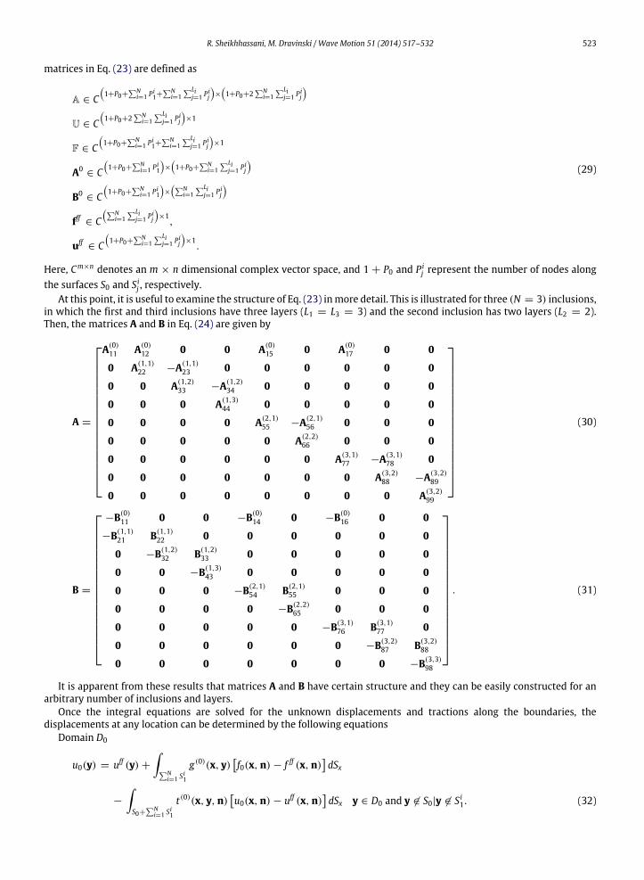
the surfaces S0 and S ij , respectively.At this point, it is useful to examine the structure of Eq. (23) inmore detail. This is illustrated for three (N = 3) inclusions,

in which the first and third inclusions have three layers (L1 = L3 = 3) and the second inclusion has two layers (L2 = 2).Then, the matrices A and B in Eq. (24) are given by

A =

A(0)11 A(0)

12 0 0 A(0)15 0 A(0)

17 0 0

0 A(1,1)22 −A(1,1)

23 0 0 0 0 0 0

0 0 A(1,2)33 −A(1,2)

34 0 0 0 0 0

0 0 0 A(1,3)44 0 0 0 0 0

0 0 0 0 A(2,1)55 −A(2,1)

56 0 0 0

0 0 0 0 0 A(2,2)66 0 0 0

0 0 0 0 0 0 A(3,1)77 −A(3,1)

78 0

0 0 0 0 0 0 0 A(3,2)88 −A(3,2)

89

0 0 0 0 0 0 0 0 A(3,2)99

(30)

B =

−B(0)11 0 0 −B(0)

14 0 −B(0)16 0 0

−B(1,1)21 B(1,1)

22 0 0 0 0 0 0

0 −B(1,2)32 B(1,2)

33 0 0 0 0 0

0 0 −B(1,3)43 0 0 0 0 0

0 0 0 −B(2,1)54 B(2,1)

55 0 0 0

0 0 0 0 −B(2,2)65 0 0 0

0 0 0 0 0 −B(3,1)76 B(3,1)

77 0

0 0 0 0 0 0 −B(3,2)87 B(3,2)

88

0 0 0 0 0 0 0 −B(3,3)98

. (31)

It is apparent from these results that matrices A and B have certain structure and they can be easily constructed for anarbitrary number of inclusions and layers.

Once the integral equations are solved for the unknown displacements and tractions along the boundaries, thedisplacements at any location can be determined by the following equations

Domain D0

u0(y) = uff (y) +

N

i=1 Si1

g(0)(x, y)f0(x,n) − f ff (x,n)

dSx

−

S0+

Ni=1 Si1

t(0)(x, y,n)u0(x,n) − uff (x,n)

dSx y ∈ D0 and y ∈ S0|y ∈ S i1. (32)

524 R. Sheikhhassani, M. Dravinski / Wave Motion 51 (2014) 517–532

Domain Dij, 1 ≤ i ≤ N, 1 ≤ j ≤ Li−1

usc(i)j (y) = −

Sij

[g(i)j (x, y)f sc(i)j (x,n) − t(i)j (x, y,n)usc(i)

j (x)]dSx

+

Sij+1

[g(i)j (x, y)f (i)

j (x,n) − t(i)j (x, y,n)u(i)j (x)]dSx y ∈ Di

j and y ∈ S ij |y ∈ S ij+1. (33)

Domain DiLi

usc(i)Li

(y) = −

S(i)Li

[g(i)Li

(x, y)f sc(i)Li(x,n) − t(i)Li

(x, y,n)usc(i)Li

(x)]dSx y ∈ DiLi and y ∈ S iLi . (34)

This completes the discretization of the integral equations. The numerical results are considered next.

4. Numerical results

4.1. Key model properties

Without loss of generality the layer interfaces are assumed to be of an elliptical shape. A dimensionless frequency η isintroduced as

η =2aλinc

a = max(ai1); i = 1 : N(35)

where λinc is the wavelength of the incident wave and ai1 is the major principle axis of the inclusion number i. Furthermore,the following parameters are assumed

S0 = xL − xR

xL = xO1 − 10

xR = xON + 10

P0 = 20S0

P ij = 128; i = 1 : N, j = 1 : Li.

(36)

Here, S0 is the length of the half-space surface, and P0 and P ij are the number of elements used to discretize S0 and S ij surfaces,

respectively. In addition, xO1 and xON are the x-coordinates of the first and last inclusion centers, respectively.Due to the large number of parameters present in the problem, the following assumptions in regards to the materials,

the number of inclusions, and the layers are proposed.The material properties of the half-space are set to be

µ0 = β0 = 1 (37)

where µ0 and β0 denote the shear modulus and the wave speed, respectively. The material properties of the layers aredenoted by µi

j and β ij , i = 1 : N, j = 1 : Li, where N denotes the number of layered inclusions and Li represent the number

of layers for the ith inclusion. The layer materials are assumed to be either of the stiff or the soft types. For the stiff layers,

the impedance contrast isρijβ

ij

ρij+1β

ij+1

> 1, (j = 1 : Li − 1) whereas for the soft layers, the impedance contrast isρijβ

ij

ρij+1β

ij+1

< 1.

The shear modulus and the shear wave velocity for the soft layers are defined by [43]

µi(soft)j = µ0 − j

1µ(i)

Li; j = 1 : Li; i = 1 : N

βi(soft)j = β0 − j

1β(i)

Li; j = 1 : Li; i = 1 : N

1µ(i)=

56; 1β(i)

=12.

(38)

R. Sheikhhassani, M. Dravinski / Wave Motion 51 (2014) 517–532 525

(a) Cavity. (b) Pipe.

Fig. 3. (a) Comparison of the surface responses of an extremely soft circular inclusion and the circular cavity embedded within a half-space subjectedto vertical and 60° incident plane harmonic SH waves studied by [48]. Solid and dashed lines represent the results of this study, whereas the squaresand triangles denote the results of [48]. The parameters are: η = 1,N = 1, a1 = b1 = 1,O = (0, 1.5), µ0 = β0 = 1, µ1 =

1600 , β1 =

12 .

(b) Comparison of the surface responses of a pipe embedded within a half-space subjected to vertical and horizontal incident plane harmonic SH waves,as studied by [49]. Solid and dashed lines represent the results of this study, whereas the squares and circles denote the results of [49]. The parameters areη = 2,N = 1, L = 2, a1 = b1 = 1, a2 = b2 = 0.9,O = (0, 1.5), µ0 = β0 = 1, µ1 = 3, β1 = 1, µ2 =

1600 , β2 =

12 .

It is apparent from Eq. (38) that the layer properties for different inclusions are assumed to be the same. Equivalently,for the stiff layers, [43]

µi(stiff)j = µ0 + j

1µ(i)

Li; j = 1 : Li; i = 1 : N

βi(stiff)j = β0 + j

1β(i)

Li; j = 1 : Li; i = 1 : N

1µ(i)=

56; 1β(i)

=12.

(39)

For example, for the three-inclusion-triple-layered soft inclusions model, the shear modulus of layers 1–3 are given by(µi

1, µi2, µ

i3) = (13/18, 4/9, 1/6), i = 1 : 3. The corresponding velocities are (β i

1, βi2, β

i3) = (5/6, 2/3, 1/2). Similarly,

for the three-inclusion-triple-layered stiff inclusions model the shear moduli of the layers are given by (µi1, µ

i2, µ

i3) =

(23/18, 14/9, 11/6), i = 1 : 3, and the corresponding velocities are (β i1, β

i2, β

i3) = (7/6, 8/6, 3/2).

To simplify the analysis of the numerical results further, the number of inclusions is assumed to be N = 3, 5, 7, or 9.The number of inclusion layers is chosen to be Li = 3 or 5. Consequently, the following notation is adopted in denoting themodels: NNLL, where N and L represent the number of inclusions and layers, respectively. For example, N 3L3 denotes athree-inclusion-triple-layered model.

4.2. Verification of numerical results

To assess the validity of the proposed method, the BIE numerical results are compared with analytical results availablein the literature.

4.3. Circular cavity

For a circular cavity embedded in a half-space, the numerical results obtained by the present method are compared withthe analytical results of [48]. The circular cavity BIE problem is modeled by a very soft single inclusion, which has a highimpedance contrast with the surrounding material, i.e., µ1 = 1/600, β1 = 1/2, which makes the impedance contrastbetween the inclusion and the half-space to be ρ1β1

ρ0β0=

11200 .

Fig. 3(a) shows a comparison between the two results for two angles of incidence. Apparently, the results are in verygood agreement.

4.4. Circular pipe

For a circular pipe embedded in the half-space, the numerical results obtained by this model are compared with theanalytical results obtained by [49]. The circular pipe BIE problem is modeled by using a two-layer inclusion, in which

526 R. Sheikhhassani, M. Dravinski / Wave Motion 51 (2014) 517–532

Fig. 4. Surface displacement amplitude for soft three-inclusion-triple-layer model vs. one-inclusion-triple-layer model for vertical (top) and grazing(bottom) incident waves. The layer centers are located at O1 = (−3, 1.5),O2

= (0, 1.5), and O3= (3, 1.5). Similarly, the various layer principle

axes are assumed to be ai1 = bi1 = 1, ai2 = bi2 = 0.75, ai3 = bi3 = 0.5, i = 1 : 3. The material properties of the layers are specified byµi

j = µi(soft)j , β i

j = βi(soft)j ; i, j = 1 : 3. For µ

i(soft)j and β

i(soft)j , see Eq. (38).

the innermost layer has the material properties of a very soft inclusion with high impedance contrast with respect tothe half-space material. Therefore, µ2 = 1/600, β2 = 1/2. The material properties of the outermost layer are given byµ1 = 3, β1 = 1.

Fig. 3(b) illustrates very good agreement between the two results for both vertical and horizontal incident waves.This concludes the testing of the numerical results. Various layered inclusion cases are considered next.

4.5. Layered inclusions

For the layered inclusion models the effect of various parameters upon the surface motion is investigated. This includesthe role of multiple scattering, the layering, the geometry, and the impedance contrast.

4.5.1. The effect of multiple scatteringThe effect of the multiple scattering of elastic waves is investigated by comparing the surface response of a multiple

multilayered inclusions model with that of a single-layered inclusion. As stated earlier, the models involving three, five,seven, and nine elliptical inclusions with three layers are considered. The layer materials are assumed to be either of thesoft or the stiff types (see Eqs. (38) and (39)).

Three-inclusion-three-layer model vs. single-inclusion-three-layer modelFor the vertical and the grazing incidences, the surface response of the soft three-inclusions-three-layer (N 3L3) and

the single-inclusion-three-layer (N 1L3) circular models are illustrated in Fig. 4. Apparently, for the vertical incidence, thepeak surface displacement amplitude (PSDA) of the N 3L3 model is greater than that of the N 1L3 model.

For the grazing incidence, one clearly distinguishes the illuminated region (x < −5), the shadow region (x > 5), andthe region directly atop the inclusions (|x| < 5). No significant effect of multiple scattering can be seen in the illuminatedregion. Atop the inclusions, however, a strong effect of multiple scattering can be observed. In particular, the PSDA of themulti-inclusion model is greater than that of the single inclusion model. Similarly, the surface responses in the shadowregion demonstrate significant difference for the single and multiple inclusion models.

Therefore, the presented results clearly demonstrate that multiple scatteringmay become very important for the surfacemotion amplification atop the soft inclusion model.

As the material properties change from soft to stiff, the surface displacement amplification is depicted by Fig. 5. For thevertical incidence, there is a reduction of oscillatory motion amplitude in the far-field region in contrast to the soft model.Moreover, the PSDA for the multiple inclusion (N 3L3) model is greater than that of the single (N 1L3) model.

R. Sheikhhassani, M. Dravinski / Wave Motion 51 (2014) 517–532 527

Fig. 5. Surface displacement amplitude for stiff three-inclusion-triple-layer model vs. one-inclusion-triple-layer model for vertical (top) and grazing(bottom) incident waves. The parameters of the problem (see Fig. 4) are as follows: O1

= (−3, 1.5),O2= (0, 1.5),O3

= (3, 1.5), ai1 = bi1 = 1, ai2 = bi2 =

0.75, ai3 = bi3 = 0.5, µij = µ

i(stiff)j , β i

j = βi(stiff)j ; i, j = 1 : 3.

For the grazing incidence, the PSDAs for the two models are similar. However, for the N 3L3 model, the location of thePSDA is shifted to the left compared with the N 1L3 model. It is interesting to observe that there are negligible oscillationsin the illuminated regions of both models. In the shadow region, the responses for the two models attenuate similarly withdistance.

Therefore, the results of the N 3L3 and N 1L3 models can be summarized as follows:

• Multiple scattering of the elastic waves by different inclusions may strongly affect the surface motion.• The PSDA for the three-inclusion-three-layer (N 3L3) model is larger than or equal to that of the single-inclusion-three-

layer model (N 1L3).• A great reduction of oscillatory motion is present in the illuminated regions for both models.• A significant difference in the surface motion can be observed between the illuminated and the shadow regions.

Comparison of the surface response between the five-inclusion-three-layer (placed along four corners and center of asquare) and single-inclusion-three-layermodels was considered as well. These results are found to be in agreement to thosefor the three-inclusion model and thus, these figures have been omitted.

This concludes the analysis of the effect of multiple scattering in the model. The role of inclusion layering on surfacemotion is considered next.

4.5.2. The effect of layeringTo study the effect of inclusion layering on the surface motion, the response of multiple layered inclusions is compared

with that of the corresponding homogeneous inclusionsmodels. The averagedmaterial properties are assumed for the lattermodels. The results for three and five inclusions with one and three layers are considered next.

Three-inclusion-three-layer model vs. three-inclusion-single-layer averaged modelWhen the layers are made of the soft materials, the surface responses of the half-space for the N 3L3 and N 3L1avg

models are shown in Fig. 6.For the vertical incidence and atop the inclusions, the PSDA for the N 3L3 model is higher than that of the N 3L1avg

model. However, in the far-field (|x| > 5), the PSDAs of the two models are quite similar.For the grazing incidence, however, the PSDA for the averagedmodel is much higher than that of themultilayeredmodel,

in the illuminated region, and slightly higher atop the inclusions. Conversely, the PSDA of the multilayered model is overallhigher than that of the averaged model in the shadow region.

The case of layers with stiff materials is depicted in Fig. 7. Evidently, for both the vertical and the grazing incidences nosignificant difference between the layered and homogeneous models is observed.

528 R. Sheikhhassani, M. Dravinski / Wave Motion 51 (2014) 517–532

Fig. 6. Surface displacement amplitude for soft three-inclusion-triple-layer model vs. three-inclusion-single-layer model with averaged materialproperties for vertical (top) and grazing (bottom) incident waves. The parameters of the problem are: O1

= (−3, 1.5),O2= (0, 1.5),O3

= (3, 1.5), ai1 =

bi1 = 1, ai2 = bi2 = 0.75, ai3 = bi3 = 0.5, µi1 = µi

2 = µi3 =

13

3j=1 µ

i(soft)j , β i

1 = β i2 = β i

3 =13

3j=1 β

i(soft)j ; i, j = 1 : 3.

Fig. 7. Surface displacement amplitude for stiff three-inclusion-triple-layer model vs. three-inclusion-single-layer model with averaged materialproperties for vertical (top) and grazing (bottom) incident waves. The parameters of the problem are: O1

= (−3, 1.5),O2= (0, 1.5),O3

= (3, 1.5), ai1 =

bi1 = 1, ai2 = bi2 = 0.75, ai3 = bi3 = 0.5, µij =

13

3j=1 µ

i(stiff)j ; β i

j =13

3j=1 β

i(stiff)j ; i, j = 1 : 3.

R. Sheikhhassani, M. Dravinski / Wave Motion 51 (2014) 517–532 529

Fig. 8. Surface displacement amplitude for soft N 3L3 circular vs. elliptical models for vertical (top) and grazing (bottom) incident waves. The parametersof the problem are: O1

= (−3, 1.5),O2= (0, 1.5),O3

= (3, 1.5), µij = µ

i(soft)j , β i

j = βi(soft)j ; i, j = 1 : 3. For the elliptical model the principle axes

are assumed to be: ai1 = 1, bi1 = 0.75, ai2 = 0.75, bi2 = 0.56, ai3 = 0.5, bi3 = 0.38, and i = 1 : 3. For the circular model the corresponding radii areai1 = bi1 = 1, ai2 = bi2 = 0.75, and ai3 = bi3 = 0.5.

A comparison of the surface response between the five-inclusion-three-layer (placed along four corners and center of asquare) and five-inclusion-single-layer model, showed similar results and thus they are omitted to reduce the number offigures.

Therefore, the results presented demonstrate that the surface response of themodel strongly depends upon the inclusionlayering for soft materials. For the stiff materials, however, the effect of layering upon PSDA is rather small.

4.6. The effect of the layers’ geometry

The influence of the geometry of the layers can be studied by comparing the response of circular and elliptical models.The three-inclusion-three-layer model (N 3L3) with soft materials is considered. The location of the inclusions’ centers

is the same for both of these models. In addition, the major axes of the elliptical layers are the same as the radii of thecorresponding circles.

It is evident from Fig. 8 that the PSDA of the two models is similar in the far-field and atop the inclusions for the verticalincidence.

However, for the grazing incidence, the PSDAs of the elliptical inclusions are overall higher than those of the circularinclusions in the illuminated region. The PSDAs are similar atop the inclusions, anddifferent attenuation behavior is observedin the shadow region.

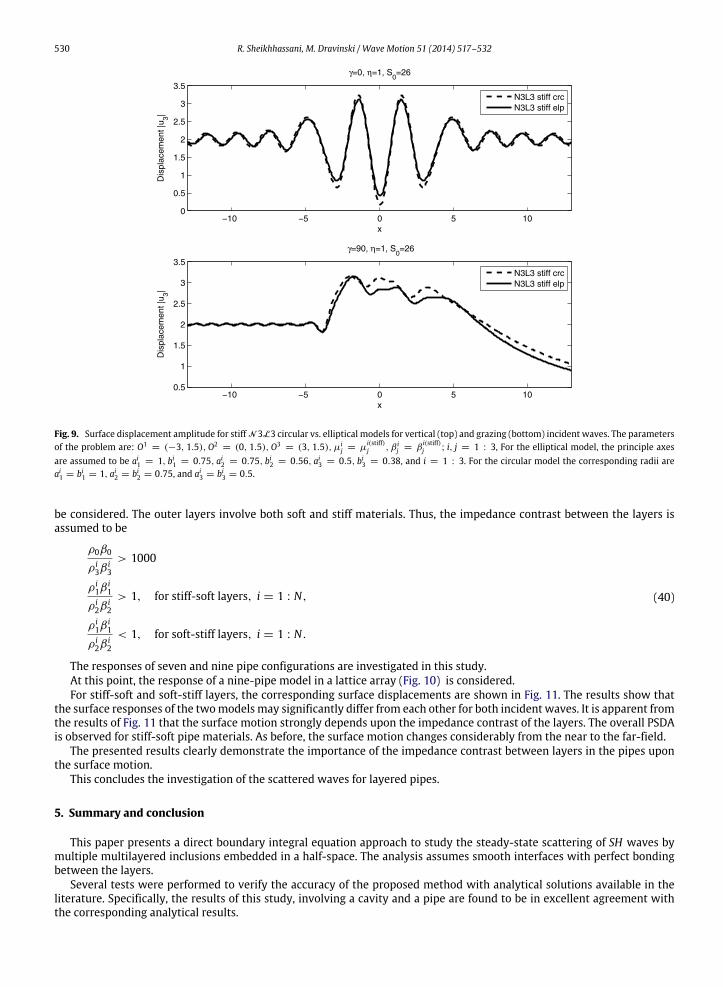
In the case of stiff materials, the difference between the PSDAs of the responses of circular and elliptical multilayeredmodels is negligible for both incidences (Fig. 9).

In summary, the presented results show that the inclusion shape affects the surface motion more for the soft materialsthan for the stiff materials.

This completes the analysis of the surface response for multilayered multiple inclusions. The cases of layered pipes areconsidered next.

4.7. The role of impedance contrast for layered pipes

The layered inclusionmodels can be extended to solve the diffraction problem by layered pipes as well. For that purpose,the innermost inclusions are assumed to be composed of an extremely soft material. Throughout, only two-layer pipes will

530 R. Sheikhhassani, M. Dravinski / Wave Motion 51 (2014) 517–532

Fig. 9. Surface displacement amplitude for stiff N 3L3 circular vs. elliptical models for vertical (top) and grazing (bottom) incident waves. The parametersof the problem are: O1

= (−3, 1.5),O2= (0, 1.5),O3

= (3, 1.5), µij = µ

i(stiff)j , β i

j = βi(stiff)j ; i, j = 1 : 3, For the elliptical model, the principle axes

are assumed to be ai1 = 1, bi1 = 0.75, ai2 = 0.75, bi2 = 0.56, ai3 = 0.5, bi3 = 0.38, and i = 1 : 3. For the circular model the corresponding radii areai1 = bi1 = 1, ai2 = bi2 = 0.75, and ai3 = bi3 = 0.5.

be considered. The outer layers involve both soft and stiff materials. Thus, the impedance contrast between the layers isassumed to be

ρ0β0

ρ i3β

i3

> 1000

ρ i1β

i1

ρ i2β

i2

> 1, for stiff-soft layers, i = 1 : N,

ρ i1β

i1

ρ i2β

i2

< 1, for soft-stiff layers, i = 1 : N.

(40)

The responses of seven and nine pipe configurations are investigated in this study.At this point, the response of a nine-pipe model in a lattice array (Fig. 10) is considered.For stiff-soft and soft-stiff layers, the corresponding surface displacements are shown in Fig. 11. The results show that

the surface responses of the twomodels may significantly differ from each other for both incident waves. It is apparent fromthe results of Fig. 11 that the surface motion strongly depends upon the impedance contrast of the layers. The overall PSDAis observed for stiff-soft pipe materials. As before, the surface motion changes considerably from the near to the far-field.

The presented results clearly demonstrate the importance of the impedance contrast between layers in the pipes uponthe surface motion.

This concludes the investigation of the scattered waves for layered pipes.

5. Summary and conclusion

This paper presents a direct boundary integral equation approach to study the steady-state scattering of SH waves bymultiple multilayered inclusions embedded in a half-space. The analysis assumes smooth interfaces with perfect bondingbetween the layers.

Several tests were performed to verify the accuracy of the proposed method with analytical solutions available in theliterature. Specifically, the results of this study, involving a cavity and a pipe are found to be in excellent agreement withthe corresponding analytical results.

R. Sheikhhassani, M. Dravinski / Wave Motion 51 (2014) 517–532 531

Fig. 10. Nine-pipe model (N = 9) configuration with the pipes centers at O1= (−2.5, 6.5),O2

= (−2.5, 4),O3= (−2.5, 1.5),O4

= (0, 6.5),O5=

(0, 4),O6= (0, 1.5),O7

= (2.5, 6.5),O8= (2.5, 4), and O9

= (2.5, 1.5). The principal axes are ai1 = bi1 = 1, ai2 = bi2 = 0.75, and ai3 = bi3 = 0.5 fori = 1 : 9.

Fig. 11. Surface displacement amplitude for nine-pipe model (see Fig. 10) for stiff-soft and soft-stiff layers for vertical (top) and grazing (bottom) incidentwaves. For the stiff-soft model: µ

i(stiff)1 = 14/9, µi(soft)

2 = 4/9, µi3 = 1/600, β i(stiff)

1 = 12/9, β i(soft)2 = 2/3, β i

3 = 1/2; i = 1 : 9. For the soft-stiff model:µ

i(soft)1 = 4/9, µi(stiff)

2 = 14/9, µi3 = 1/600; β

i(soft)1 = 2/3, β i(stiff)

2 = 12/9, β i3 = 1/2; i = 1 : 9.

The numerical results presented here for layered inclusions and pipes, can be summarized as follows:The surface motion may be greatly affected by the multiple scattering of elastic waves by the inclusions. In addition, the

surface response strongly depends upon layering for the soft materials. For the stiff inclusion materials, this dependence isnot as strong.

The effect of inclusion shape upon the surface motion is more pronounced for the soft inclusion layers than for the stiffinclusion layers.

For the grazing incidence, the highly oscillatorymotion in the illuminated portion of the far-field is greatly reducedwhenthe soft inclusion layers are replaced by the stiff layers.

532 R. Sheikhhassani, M. Dravinski / Wave Motion 51 (2014) 517–532

For the layered pipes, the surface motion is found to be strongly dependent upon the impedance contrast between thelayers. In addition, the surface response changes considerably from the near to the far-field.

Consequently, the presented results clearly demonstrate the importance of the scattering of SH waves by multiplemultilayered inclusions upon the surface response.

References

[1] O. Gericke, Determination of the geometry of hidden defects by ultrasonic pulse analysis testing, J. Acoust. Soc. Am. 35 (1963) 364.[2] F. Cohen-Tenoudji, B. Tittmann, G. Quentin, Technique for the inversion of backscattered elastic wave data to extract the geometrical parameters of

defects with varying shape, Appl. Phys. Lett. 41 (1982) 574–576.[3] G.J. Muller, Medical Optical Tomography Functional Imaging and Monitoring, SPIE Optical Engineering Press, 1993.[4] V.V. Tuchin, Tissue Optics: Light Scattering Methods and Instruments for Medical Diagnosis, SPIE Press, Bellingham, Wash., 2007.[5] J. Hudson, J. Heritage, The use of the born approximation in seismic scattering problems, Geophys. J. Int. 66 (1981) 221–240.[6] R.-S. Wu, Multiple scattering and energy transfer of seismic waves-separation of scattering effect from intrinsic attenuation-I. Theoretical modelling,

Geophys. J. Int. 82 (1985) 57–80.[7] P.A. Martin, Multiple Scattering: Interaction of Time-Harmonic Waves with N Obstacles, vol. 107, Cambridge University Press, 2006.[8] L.L. Foldy, The multiple scattering of waves, Phys. Rev. 67 (1945) 107–119.[9] M. Lax, Multiple scattering of waves, II. The effective field in dense systems, Phys. Rev. 85 (1952) 621.

[10] V. Twersky, Multiple scattering of radiation by an arbitrary configuration of parallel cylinders, J. Acoust. Soc. Am. 24 (1952) 42.[11] V. Twersky, Multiple scattering by arbitrary configurations in three dimensions, J. Math. Phys. 3 (1962) 83.[12] P.C. Waterman, R. Truell, Multiple scattering of waves, J. Math. Phys. 2 (1961) 512.[13] P. Waterman, Matrix formulation of electromagnetic scattering, Proc. IEEE 53 (1965) 805–812.[14] B. Peterson, S. Ström, Tmatrix for electromagnetic scattering from an arbitrary number of scatterers and representations of e (3), Phys. Rev. D 8 (1973)

3661.[15] B. Peterson, S. Ström, Matrix formulation of acoustic scattering from an arbitrary number of scatterers, J. Acoust. Soc. Am. 56 (1974) 771.[16] B. Peterson, S. Ström, T-matrix formulation of electromagnetic scattering from multilayered scatterers, Phys. Rev. D 10 (1974) 2670.[17] B. Peterson, S. Ström, Matrix formulation of acoustic scattering from multilayered scatterers, J. Acoust. Soc. Am. 57 (1975) 2.[18] S. Bose, A. Mal, Longitudinal shear waves in a fiber-reinforced composite, Int. J. Solids Struct. 9 (1973) 1075–1085.[19] V. Varadan, Y. Ma, V. Varadan, A multiple scattering theory for elastic wave propagation in discrete randommedia, J. Acoust. Soc. Am. 77 (1985) 375.[20] J.G. Berryman, Long-wavelength propagation in composite elastic media I. Spherical inclusions, J. Acoust. Soc. Am. 68 (1980) 1809.[21] F.J. Sabina, J. Willis, A simple self-consistent analysis of wave propagation in particulate composites, Wave Motion 10 (1988) 127–142.[22] R.-B. Yang, A.K. Mal, Multiple scattering of elastic waves in a fiber-reinforced composite, J. Mech. Phys. Solids 42 (1994) 1945–1968.[23] S.K. Kanaun, Self-consistent methods in the problem of wave propagation through heterogeneous media, in: Heterogeneous Media, Springer, 2000,

pp. 241–319.[24] R.-B. Yang, A.K. Mal, Elastic waves in a composite containing inhomogeneous fibers, Internat. J. Engrg. Sci. 34 (1996) 67–79.[25] R.M. Christensen, A critical evaluation for a class of micro-mechanics models, J. Mech. Phys. Solids 38 (1990) 379–404.[26] S. Kanaun, V. Levin, Effective mediummethod in the problem of axial elastic shear wave propagation through fiber composites, Int. J. Solids Struct. 40

(2003) 4859–4878.[27] P. Wei, Z. Huang, Dynamic effective properties of the particle-reinforced composites with the viscoelastic interphase, Int. J. Solids Struct. 41 (2004)

6993–7007.[28] S. Biwa, S. Yamamoto, F. Kobayashi, N. Ohno, Computational multiple scattering analysis for shear wave propagation in unidirectional composites,

Int. J. Solids Struct. 41 (2004) 435–457.[29] T. Sumiya, S. Biwa, G. Haïat, Computational multiple scattering analysis of elastic waves in unidirectional composites, Wave Motion (2013).[30] Z. Ou, D. Lee, Effects of interface energy on scattering of plane elastic wave by a nano-sized coated fiber, J. Sound Vib. (2012).[31] G. Beer, I.M. Smith, C. Duenser, The Boundary Element Method with Programming: For Engineers and Scientists, Springer, 2008.[32] M. Aliabadi, The Boundary Element Method, vol. 2, in: Applications in Solids and Structures, Wiley, London, 2002.[33] R. Clayton, B. Engquist, Absorbing boundary conditions for acoustic and elastic wave equations, Bull. Seismol. Soc. Amer. 67 (1977) 1529–1540.[34] C.A. Brebbia, The Boundary Element Method for Engineers, Wiley, New York, 1978.[35] M. Dravinski, Scattering of SH waves by subsurface topography, J. Eng. Mech. Div. 108 (1982) 1–17.[36] O. Coutant, Numerical study of the diffraction of elastic waves by fluid-filled cracks, J. Geophys. Res.: Solid Earth 94 (1989) 17805–17818 (1978–2012).[37] H. Kawase, Time-domain response of a semi-circular canyon for incident SV, P, and Rayleigh waves calculated by the discrete wavenumber boundary

element method, Bull. Seismol. Soc. Amer. 78 (1988) 1415–1437.[38] G.D. Manolis, D.E. Beskos, Boundary Element Methods in Elastodynamics, Unwin Hyman, London, Boston, 1988.[39] R. Benites, K. Aki, K. Yomogida, Multiple scattering of SH waves in 2-D media with many cavities, Pure Appl. Geophys. 138 (1992) 353–390.[40] R.A. Benites, P.M. Roberts, K. Yomogida, M. Fehler, Scattering of elastic waves in 2-d composite media I. Theory and test, Phys. Earth Planet. Inter. 104

(1997) 161–173.[41] J. DeSanto, Theory of scattering from multilayered bodies of arbitrary shape, Wave Motion 2 (1980) 63–73.[42] M. Dravinski, M.C. Yu, Scattering of plane harmonic SH waves by multiple inclusions, Geophys. J. Int. 186 (2011) 1331–1346.[43] M. Dravinski, R. Sheikhhassani, Scattering of a plane harmonic {SH}wave by a roughmultilayered inclusion of arbitrary shape,WaveMotion 50 (2013)

836–851.[44] K. Graff, Wave Notion in Elastic Solids, in: Dover Books on Engineering Series, Dover Publications, Incorporated, 1975.[45] Y. Niu, M. Dravinski, Direct 3D bem for scattering of elastic waves in a homogeneous anisotropic half-space, Wave Motion 38 (2003) 165–175.[46] S. Kobayashi, Elastodynamics, in: Boundary Element Methods in Mechanics, North-Holland, 1987. Sole distributors for the USA and Canada, Elsevier

Science Pub. Co., Amsterdam, New York, NY, USA.[47] F. París, J. Cañas, Boundary Element Method: Fundamentals and Applications, in: Oxford Science Publications, vol. 1, Oxford University Press, 1997.[48] V. Lee, On deformations near circular underground cavity subjected to incident plane SH waves, in: Proceedings of the Application of Computer

Methods in Engineering Conference, vol. 2, Los Angeles, pp. 951–962.[49] M.E. Manoogian, Scattering and diffraction of SH waves above an arbitrarily shaped tunnel, ISET J. Earthq. Technol. 37 (2000) 11–26.