
Enron Broadband Services Jeff Skilling President & CEO-Elect Enron Corp.

Scan Statistics on Enron Graphs∗
Carey E. PriebeJohns Hopkins University, Baltimore, MD
John M. ConroyIDA Center for Computing Sciences, Bowie, MD
David J. MarchetteNSWC B10, Dahlgren, VA
Youngser ParkJohns Hopkins University, Baltimore, MD
May 10, 2005
Word count: 3370
Character count: 21765
Previous presentation: Workshop on Link Analysis, Counterterrorism and Security at the
SIAM International Conference on Data Mining, Newport Beach, CA, April 23, 2005
Abstract
We introduce a theory of scan statistics on graphs and apply the ideas to
the problem of anomaly detection in a time series of Enron email graphs.∗Corresponding author: Carey E. Priebe = <[email protected]>
– 1–

1 Introduction.
Consider a directed graph (digraph) D with vertex set V (D) and arc set A(D)
of directed edges. For instance, we may think of D as a communications or so-
cial network, where the n = |V (D)| vertices represent people or computers or
more general entities and an arc (v, w) ∈ A(D) from vertex v to vertex w is to be
interpreted as meaning “the entity represented by vertex v is in directed commu-
nication with or has a directed relationship with the entity represented by vertex
w.” We are interested in testing the null hypothesis of “homogeneity” against al-
ternatives suggesting “local subregions of excessive activity.” Toward this end, we
develop and apply a theory of scan statistics on random graphs.
2 Scan Statistics.
Scan statistics are commonly used to investigate an instantiation of a random field
X (a spatial point pattern, perhaps, or an image of pixel values) for the possi-
ble presence of a local signal. Known in the engineering literature as “moving
window analysis”, the idea is to scan a small window over the data, calculating
some local statistic (number of events for a point pattern, perhaps, or average
pixel value for an image) for each window. The supremum or maximum of these
locality statistics is known as the scan statistic, denoted M(X). Under some spec-
ified “homogeneity” null hypothesis H0 on X (Poisson point process, perhaps, or
Gaussian random field) the approach entails specification of a critical value cα
such that PH0[M(X) ≥ cα] = α. If the maximum observed locality statistic
is larger than or equal to cα, then the inference can be made that there exists a
nonhomogeneity — a local region with statistically significant signal.
– 2–

An intuitive approach to testing these hypotheses involves the partitioning of
the region X into disjoint subregions. For cluster detection in spatial point pro-
cesses this dates to Fisher’s 1922 “quadrat counts” [Fisher and Mackenzie, 1922];
see [Diggle, 1983]. Absent prior knowledge of the location and geometry of po-
tential nonhomogeneities, this approach can have poor power characteristics.
Analysis of the univariate scan process (d = 1) has been considered by many
authors, including [Naus, 1965], [Cressie, 1977], [Cressie, 1980], and [Loader, 1991].
For a few simple random field models exact p−values are available; many ap-
plications require approximations to the p−value. The generalization to spatial
scan statistics is considered in [Naus, 1965], [Adler, 1984], [Loader, 1991], and
[Chen and Glaz, 1996]. As noted by [Cressie, 1993], exact results for d = 2 have
proved elusive; approximations to the p−value based on extreme value theory are
in general all that is available. [Naiman and Priebe, 2001] present an alternative
approach, using importance sampling, to this problem of p−value approximation.
3 Scan Statistics on Graphs.
The order of the digraph, n = |V (D)|, is the number of vertices. The size of the
digraph, |A(D)|, is the number of arcs. For v, w ∈ V (D) the digraph distance
d(v, w) is defined to be the minimum directed path length from v to w in D.
For non-negative integer k (the scale) and vertex v ∈ V (D) (the location),
consider the closed kth-order neighborhood of v in D, denoted Nk[v; D] = w ∈
V (D) : d(v, w) ≤ k. We define the scan region to be the induced subdigraph
thereof, denoted
Ω(Nk[v; D])(1)
– 3–

with vertices V (Ω(Nk[v; D])) = Nk[v; D] and arcs A(Ω(Nk[v; D])) = (v, w) ∈
A(D) : v, w ∈ Nk[v; D]. A locality statistic at location v and scale k is any
specified digraph invariant Ψk(v) of the scan region Ω(Nk[v; D]). For concrete-
ness consider for instance the size invariant, Ψk(v) = |A(Ω(Nk[v; D]))|. Notice,
however, that any digraph invariant (e.g. density, domination number, etc.) may be
employed as the locality statistic, as dictated by application. The “scale-specific”
scan statistic Mk(D) is given by some function of the collection of locality statis-
tics Ψk(v)v∈V (D); consider for instance the maximum locality statistic over all
vertices,
Mk(D) = maxv∈V (D)
Ψk(v).(2)
This idea is introduced in [Priebe, 2004].
Under a null model for the random digraph D (for instance, the Erdos-Renyi
random digraph model) the variation of Ψk(v) can be characterized and Mk(D)
large indicates the existence of an induced subdigraph (scan region) Ω(Nk[v; D])
with excessive activity. A test can be constructed for a specific alternative of
interest concerning the structure of the excessive activity anticipated. However, if
the anticipated alternative is, more generally, some form of “chatter” in which one
(small) subset of vertices communicate amongst themselves (in either a structured
or an unstructured manner) then our scan statistic approach promises more power
than other approaches.
Finally, we wish to consider the scan statistic which accounts for variable
scale. Let K ⊂ 1, · · · , n − 1 be a collection of scales, and let Ψ′
k be a scale-
standardized version of the locality statistic Ψk. For instance, for given α ∈ (0, 1),
find gk,α(·) such that Ψ′
k(v) = gk,α(Ψk(v)) satisfies P [Ψ′
k(v) ≥ cα] ≈ α for all
v ∈ V (D) and for all k ∈ K. This standardization imposes upon each locality
– 4–

statistic the same probability of exceedance. Then the scan statistic MK(D) is
given by
MK(D) = maxk∈K
maxv∈V (D)
Ψ′
k(v)(3)
and we reject for large values of MK(D).
For the Enron data considered in this paper, as for much social network data,
no appropriate simple null random graph model is obvious. The dataset, as we
process it, consist of a time series of digraphs D1, D2, · · · , DT=189. We will pro-
ceed conditionally: we will assume that the data (or the statistics derived from
the data) have some short-time stationarity properties under the null, so that a
moving window approach is appropriate. We will be concerned with discovering
anomalies that appear as digraphs which differ substantially from those seen in the
recent past. In particular, we wish to detect subdigraphs with an unusually high
connectivity, as measured by our statistic. This conditional approach alleviates
the requirement to posit an appropriate and simple null graph model — but does
require some (approximate) stationarity.
4 The Enron Data.
The Enron email dataset is available online [enr, b]. This dataset consists of a col-
lection of 150 folders corresponding to the email to and from senior management
and others at Enron, collected over a period from about 1998 to 2002. The emails
have been minimally processed to correct integrity problems. Some emails have
been deleted, as have all attachments. Thus, while imperfect, this dataset repre-
sents a rich environment in which to perform text analysis and link analysis. More
information on this dataset can be found online [enr, a].
– 5–

One consequence of the processing of these data is that some of the orig-
inal email addresses have been changed. Invalid addresses were converted to
no [email protected]. In several cases, individuals have multiple addresses,
which are clearly a result of some post-processing: for example, John Q. Public
has email addresses [email protected] and [email protected]. In this
study we will treat such cases as distinct; one potential goal might be to recognize
this “aliasing” from the link analysis alone, without reference to the content of the
messages. This will be discussed further in Section 7.1.
5 Whence Our Enron Graphs?
The data are collected from “about 150 users” — mostly Enron executives, but
also some energy traders, executive assistants, etc. However, our graphs are based
on 184 users, which is the number of unique addresses we obtain from the ‘From’
line of emails in the ‘Sent’ boxes after manually removing some addresses which
are clearly not associated with the 150 users. (NB: Neither of the two extreme
options — keeping all addresses, or merging to the point of one-to-one correspon-
dence between addresses and known users — seems practical; the former yields
too many obvious aliases and extraneous addresses, and no simple unassailable
version of the latter presents itself to us. Thus, we proceed with an admittedly
imperfect collection of vertices.) In addition, some of the time stamps in the orig-
inal data are clearly invalid, occurring before Enron existed, so we restrict our
attention to a period of 189 weeks, from 1998 through 2002.
For each week t = 1, · · · , 189, there is a digraph Dt = (V, At) with |V | = 184
vertices and directed edges (arcs) At, where (v, w) ∈ At ⇐⇒ vertex v sends at
– 6–
least one e-mail to vertex w during the t-th week. We make no distinction between
emails sent “To”, “CC” or “BCC”.
6 Statistics and Time Series.
Our time-dependent scale-k locality statistic is given by
Ψk,t(v) = |A(Ω(Nk[v; Dt]))|(4)
for k ∈ 1, 2, · · · , K. In an abuse of notation, we will let Ψ0,t(v) = outdegree(v; Dt).
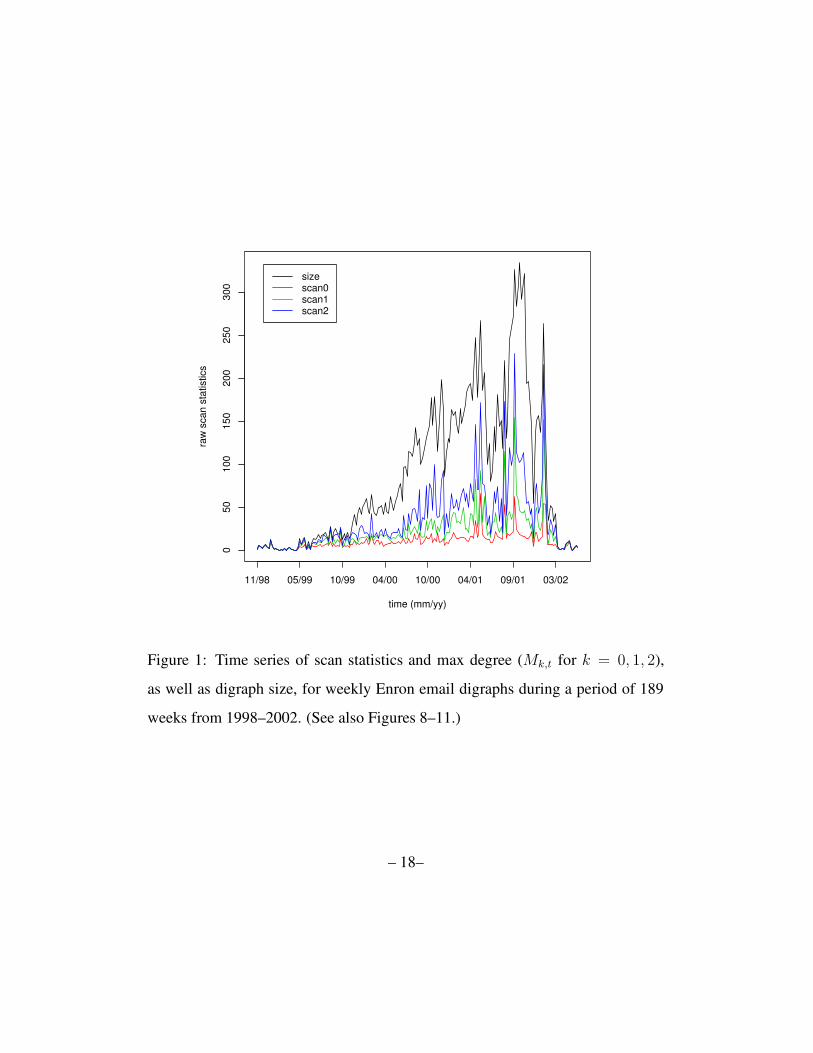
Figure 1 shows the three statistics
Mk,t = maxv
Ψk,t(v); k = 0, 1, 2(5)
as well as size(Dt), as functions of time (weeks) t = 1, · · · , 189 for the 189
weeks under consideration. (Figures 8–11 show these four curves separately.)
The raw locality statistics Ψk,t(v) are inadequate for our purposes. Con-
sider, for instance, the situation in which one vertex, v, has a lot of activity
throughout time, and another vertex, w, has but one tenth this amount of activ-
ity until one week in which w triples its activity. Without some form of vertex-
dependent standardization, the increase in activity for w will go unnoticed, as
v = arg max Ψk,t(v) regardless of w’s increased activity. Thus the locality statis-
tics Ψk,t(v) must be standardized using vertex-dependent recent history.
Our vertex-standardized locality statistic, for k = 0, 1, 2, is given by
Ψk,t(v) = (Ψk,t(v) − µk,t,τ (v)) / max(σk,t,τ(v), 1)(6)
where
µk,t,τ(v) =1
τ
t−1∑
t′=t−τ
Ψk,t′(v)(7)
– 7–

and
σ2k,t,τ (v) =
1
τ − 1
t−1∑
t′=t−τ
(Ψk,t′(v) − µk,t,τ(v))2.(8)
That is, we standardize the locality statistic Ψk,t(v) by a vertex-dependent mean
and standard deviation based on recent history. (The denominator in Ψk,t(v) is
forced to be greater than or equal to one to eliminate fragility due to vertices with
little or no variation in activity.)
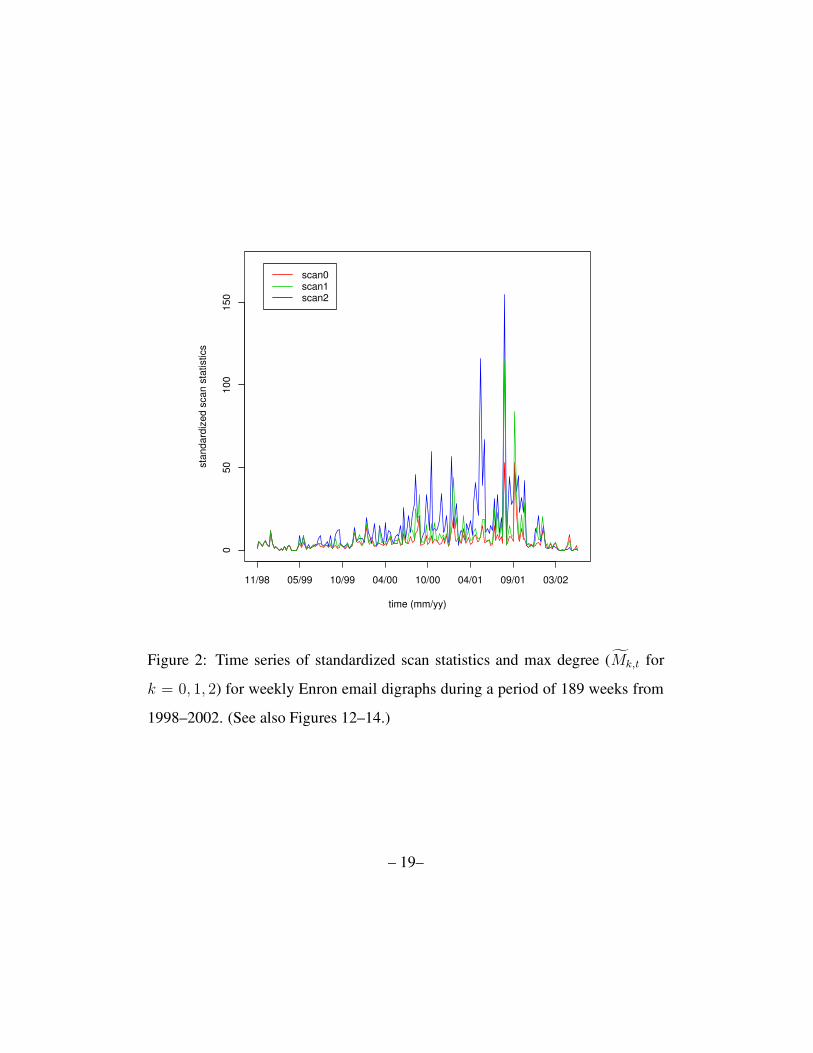
In Figure 2 we plot the standardized scan statistics
Mk,t = maxv
Ψk,t(v)(9)
against t over the 189 weeks. (Figures 12–14 show these three curves separately.)
This approach requires a vertex-dependent local stationarity assumption. The
validity of a stationarity assumption is obviously suspect over the entire 189 weeks,
but short-time near-stationarity (we use τ = 20) may be reasonable as a null
model.
7 Anomaly Detection.
Given the standardized scan statistic time series Mk,t presented in Figure 2, we
now consider anomaly detection.
For simplicity, we consider a temporally-normalized version of Mk,t,
Sk,t = (Mk,t − µk,t,`)/ max(σk,t,`, 1),(10)
where µk,t,` and σk,t,` are the running mean and standard deviation estimates of
Mk,t based on the most recent ` time steps. (Here we use ` = 20.) Detections are
– 8–
defined here as weeks for which Mk,t achieves a value greater than five standard
deviations above its mean; i.e., times t such that Sk,t > 5
Figure 3 depicts S2,t for a 20 week period from February 2001 through June
2001. We observe that the second order scan statistic indicates a clear anomaly at
t∗ = 132 (maxv Ψ2,132(v) is a seven sigma event) in May 2001. This anomaly is
apparent, in hindsight, in Figure 2.
Inference performed using simple sigmages is inadequate in this case, of course,
because there is no reason to believe that the distribution of Sk,t is normal or
that Sk,t and Sk,t′ are independent. Computational methods such as the bootstrap
would be appropriate. We consider exceedance probabilities of an extreme value
distribution, the Gumbel, fit via the method of moments. S2,132 = 7.3; 7.3 stan-
dard deviations yields a p−value < 10−10, assuming normality. While the signif-
icance for the detection at t∗ = 132 is not so drastic under the more reasonable
Gumbel model, we nevertheless obtain an exceedance probability < 10−6, which
remains convincing. Bonferonni analysis suggests that if the Ψk,t are approxi-
mately distributed as a t19 then the detection is significant; however, if the distri-
bution of the Ψk,t has extraordinarily heavy tails (e.g., Cauchy) then the α = 0.05
level critical value may be greater than 7.3. Thus, under a reasonable range of null
distributions, the detection at t∗ = 132 is statistically significant.
Figure 4 shows the graph topology, sans isolates, for our ‘detection’ graph
D132. Our vertex of interest, v∗ = arg maxv Ψ2,132(v), is identified with email
address email90. Of note is the fact that arg maxv Ψ0,132(v) = email83. That is,
the vertex of maximum outdegree for t∗ = 132 is not the cause of our detection.
Furthermore, arg maxv Ψ1,132(v) = email83, arg maxv Ψ2,132(v) = email147,
arg maxv Ψ0,132(v) = email147, and arg maxv Ψ1,132(v) = email75. Thus the
– 9–

detection based on v∗ = email90 is apparent only when using the standardized
second order scan statistic.
Table 1 gives some relevant numerical values for the ‘detection’ graph D132.
There is excessive activity among the elements of the closed 2-neighborhood
of our vertex of interest v∗ which is not accounted for by its outdegree (or its
closed 1-neighborhood). In fact, v∗ communicates, in particular, with other ver-
tices each of which has high outdegree. This type of excessive local activity is
precisely the raison d’etre for our scan statistics; our approach exhibits the ability
to detect this anomaly.
Is this detection an event of interest? It is statistically significant, but the objec-
tive of our scan statistic methodology is to sift through massive communications
data to find potentially informative events for the purpose of directing additional,
more time consuming investigations. The ultimate determination of the practi-
cal significance of this or any detection must be made on the basis of subsequent
analysis. There is a coinciding insider trading event on the Enron time line . . .
but there are many insider trading events on the Enron time line! Ideally, one
would hope to find a link between the detected excess activity and that insider
trading. Such a forensic analysis will require delving into the content of the email
messages and associated meta-data.
Time t∗ = 132 is the only week among the 189 under consideration for which
S2,t ≥ 5. Detections for the other scan statistics — orders 0, 1, and 3 — that may
be worth pursuing are summarized here. For maximum standardized outdegree,
there are three weeks with S0,t ≥ 5: 58 (week of December 16, 1999), 96 (week
of September 7, 2000), 146 (week of August 23, 2001) for the standardized first
order scan statistic, we obtain (almost) the same three detections: 58, 94, 146.
– 10–

The standardized third order scan statistic produces detections at t∗ = 132 and at
week 87.
7.1 Aliasing.
In the case of the detection at t∗ = 132,
v∗ = arg maxv
Ψ2,132(v) = email90,(11)
perusal of the emails shows that email90 and email141 are really the same per-
son. User email90 had no activity before t∗ = 132, at which time email141
switched to the email90 identifier. Thus we have detected an instance of alias-
ing, which could perhaps have been addressed during the manual merging stage
wherein we settled on the collection of 184 vertices to consider. Of course, this
identification does in fact require perusal of the emails, which perusal was sug-
gested by the detection . . . precisely the point of the exercise!
However, it may be possible to automatically identify such aliasing events.
Given the detection (v∗, t∗) we can immediately identify email90 as having had
no activity prior to t∗ = 132. From this point, we may employ a “matched filter”
scheme to determine candidates for aliasing by matching the pattern of email90’s
activity at or after t∗ = 132 against the pattern of other vertices’ activity prior to
t∗ = 132. Vertices with a high score for some matching function will be deemed
likely candidates for further investigation.
For instance, we may compute, for each vertex v ∈ V \ v∗, the simple score
st∗,κ(v; v∗) =
t∗−1∑
t′=t∗−κ
|N1(v; Dt′) ∩ N1(v∗; Dt∗)|.(12)
– 11–

In this case we obtain email141 = arg maxv st∗,κ(v; v∗) with κ ≥ 5. That is, for
this simple case, the aliasing can be automatically identified and resolved.
This idea of employing matched filters to time series of graphs, introduced
here in a very simplistic fashion, will be pursued in more detail elsewhere.
7.2 Another Detection.
The detection of v∗ = arg maxv Ψ2,132(v) = email90 at t∗ = 132, while real and
interesting, is due to the fact that email90 had not been active prior to t∗ = 132.
We may be interested, instead, in detections for which activity increases from a
non-zero baseline. That is, we consider the statistic
Ψk,t(v) · Iµ0,t,τ (v) > c,(13)
where IE is the indicator function taking value one if event E occurs and taking
value zero otherwise, which requires there to have been some recent activity.
For c = 1, one such detection of this type, for which the order k = 2 scan
statistic detects but the order k = 0 and k = 1 scan statistics do not detect, is
v∗ = email152 at t∗ = 152 (the week of October 4, 2001).
Table 2 gives the scan statistics for this detection for the weeks up to and
including t∗. Here we see clearly the increase in activity, and we see that it is not
due to order 0 or order 1 locality statistics. (N.B. It does appear that a detection at
t∗ − 2 may be appropriate.)
However, further investigation indicates that this detection is due to the fact
that email152 communicates with email154, and email154 is an order 0 locality
statistic detection at t∗ = 152 due to a massive increase in outdegree (see Table
3).
– 12–

Thus, in some sense, neither the email90 / email141 detection at t∗ = 132
nor the email152 / email154 detection at t∗ = 152 is really due to the type of
excessive “chatter” in which we are most interested.
7.3 Detecting Chatter.
For each time t and vertex v, consider the order 2 statistic
Ψ′
t(v) =(Ψ2,t(v) · It,τ (v)
)/ max(γt(v), 1).(14)
Here the term It,τ (v) is the product of three indicator functions,
Iµ0,t,τ > c1,(15)
IΨ0(v) < σ0,t,τ (v)c2 + µ0,t,τ (v),(16)
IΨ1(v) < σ1,t,τ (v)c3 + µ1,t,τ (v).(17)
That is, we gate the second order scan statistic so that some minimal level of
recent activity is required, and we insist that the order 0 and order 1 scan statistics
do not yield detections. In this way we narrow the class of alternatives under
consideration — the types of anomalous activities that will be deemed detections;
we seek a detection in which the excess activity is due to chatter amongst the 2-
neighbors. We include an “inhomogeneity penalty” γt(v), the standard deviation
of the outdegrees of the neighbors N1(v∗; Dt∗), in the denominator of Ψ′
t(v) to
further narrow our search to the case of “balanced chatter” (and to rule out events
such as the email152 / email154 detection at t∗ = 152).
The arg max(v,t) Ψ′
t(v) is given by (v∗, t∗) = (email164, 109). (The value
of t∗ = 109 corresponds to the week of December 7, 2000.) Figure 5 displays
M ′
t = maxv Ψ′
t(v) as well as the temporally-normalized version S ′
t.
– 13–

The raw locality statistics Ψk,t(v∗) for the time range t∗ − 5, · · · , t∗ leading
up to this detection are given in Table 4. As can be seen from Table 4, the raw
locality statistics for k = 0 and k = 1 do not have a substantial signal at t∗ = 109,
while for k = 2 the presence of an anomaly is clear.
The inhomogeneity penalty for this detection is γt∗(v∗) ≈ 1.7; the outdegrees
of the five neighbors of v∗ = email164 are 6,6,6,7,10.
The induced subdigraph at t∗ = 109, Ω(N2[v∗; Dt∗]), is depicted in Figure 6.
We see that v∗ = email164 has five neighbors, each of which has outdegree be-
tween six and ten. That is, this detection is due to v∗ communicating with a moder-
ate subset of vertices, each of whom communicates with another moderate subset.
Comparing this graph with email164’s induced subdigraph Ω(N2[v∗; Dt∗−1]) at
t∗ − 1 = 108 (black arcs and associated vertices in Figure 7) gives a clear, albeit
simplistic, indication that change has occurred. Figure 7 gives additional infor-
mation regarding this change, depicting the subdigraph induced at t∗ − 1 = 108
by the union of email164’s 2-neighborhood at t∗ − 1 = 108 and email164’s 2-
neighborhood at t∗ = 109. The arcs corresponding to communications between
members of email164’s closed 2-neighborhood at t∗ − 1 = 108 are depicted
in black; gray arcs represent other communications in D108 between vertices in
email164’s 2-neighborhood at t∗ = 109. Figure 7 shows that this detection is
not the result of a simple increase in the size of v∗’s neighborhood, but that the
vertices in the neighborhood at t∗, while active at t∗ − 1, have also increased their
activity. Thus, the detection is not due solely to v∗ joining a larger group; in addi-
tion, the group itself is more active as well. We interpret this figure as suggesting
that this detection is robust — insensitive to small changes in the graph.
– 14–
8 Discussion.
A theory of scan statistics on graphs offers promise for detecting anomalies in
time series of graphs.
We have employed perhaps overly-simplistic time series and inference meth-
ods, for purposes of illustration; more elaborate methods such as exponential
smoothing, detrending, and variance stabilization may be appropriate. In addi-
tion, multivariate time series (one time series for each vertex v, in this case) have
a theory all their own — e.g., vector autoregressive models — which we have
ignored here. And, of course, for data such as this Enron corpus, robust versions
of moment estimates we have employed are called for.
Nevertheless, despite our simplistic approach to these various issues, we have
demonstrated the potential utility of the scan statistic approach to the problem of
anomaly detection in a time series of Enron email graphs. Much remains to be
done — mathematically, computationally, and with respect to data and meta-data
analysis. Of particular interest is the extension of these scan statistics to weighted
graphs (and hypergraphs), allowing for the detection of anomalies related to the
number (and possibly type) of messages sent, as opposed to the simpler case con-
sidered herein.
Noteworthy as a closing fact is that the procedures introduced herein can all
be performed in a real-time, streaming data environment. That is, a sliding one-
week window, rather than disjoint one-week windows, can be utilized and nothing
presented herein causes a common laptop computer difficulty in keeping up. Thus,
these procedures can be applied in scenarios of on-line analysis, in addition to the
forensic scenario offered by this Enron corpus.
– 15–

References
[enr, a] http://www-2.cs.cmu.edu/ enron.
[enr, b] http://www.cs.queensu.ca/home/skill/siamworkshop.html.
[Adler, 1984] Adler, R. J. (1984). The supremum of a particular gaussian field.
In Annals of Probability, volume 12, pages 436–444.
[Chen and Glaz, 1996] Chen, J. and Glaz, J. (1996). Two-dimensional discrete
scan statistics. In Statistics and Probability Letters, volume 31, pages 59–68.
[Cressie, 1977] Cressie, N. (1977). On some properties of the scan statistic on
the circle and the line. In Journal of Applied Probability, volume 14, pages
272–283.
[Cressie, 1980] Cressie, N. (1980). The asymptotic distribution of the scan statis-
tic under uniformity. In Annals of Probability, volume 8, pages 828–840.
[Cressie, 1993] Cressie, N. (1993). Statistics for Spatial Data. John Wiley, New
York.
[Diggle, 1983] Diggle, P. (1983). Statistical Analysis of Spatial Point Patterns.
Academic Press, New York.
[Fisher and Mackenzie, 1922] Fisher, R.A., T. H. and Mackenzie, W. (1922). The
accuracy of the plating method of estimating the density of bacterial popula-
tions, with particular reference to the use of thornton’s agar medium with soil
samples. In Annals of Applied Biology, volume 9, pages 325–359.
– 16–

[Loader, 1991] Loader, C. (1991). Large-deviation approximations to the distri-
bution of scan statistics. In Advances in Applied Probability, volume 23, pages
751–771.
[Naiman and Priebe, 2001] Naiman, D. and Priebe, C. (2001). Computing scan
statistic p–values using importance sampling, with applications to genetics and
medical image analysis. In Journal of Computational and Graphical Statistics,
volume 10, pages 296–328.
[Naus, 1965] Naus, J. (1965). Clustering of random points in two dimensions. In
Biometrika, volume 52, pages 263–267.
[Priebe, 2004] Priebe, C. (2004). Scan statistics on graphs. Technical Report 650,
Johns Hopkins University, Baltimore, MD 21218-2682.
– 17–
050
100
150
200
250
300
time (mm/yy)
raw
scan
sta
tistic
s
11/98 05/99 10/99 04/00 10/00 04/01 09/01 03/02
sizescan0scan1scan2
Figure 1: Time series of scan statistics and max degree (Mk,t for k = 0, 1, 2),
as well as digraph size, for weekly Enron email digraphs during a period of 189
weeks from 1998–2002. (See also Figures 8–11.)
– 18–
050
100
150
time (mm/yy)
stan
dard
ized
scan
sta
tistic
s
11/98 05/99 10/99 04/00 10/00 04/01 09/01 03/02
scan0scan1scan2
Figure 2: Time series of standardized scan statistics and max degree (Mk,t for
k = 0, 1, 2) for weekly Enron email digraphs during a period of 189 weeks from
1998–2002. (See also Figures 12–14.)
– 19–

−20
24
68
time (mm/yy)
scan
0
02/01 03/01 04/01 05/01 06/01
−20
24
68
time (mm/yy)
scan
1
02/01 03/01 04/01 05/01 06/01
−20
24
68
time (mm/yy)
scan
2
02/01 03/01 04/01 05/01 06/01
Figure 3: Sk,t, the temporally-normalized standardized scan statistics, on zoomed-
in time series of Enron e-mail graphs during a period of 20 weeks in 2001. Top:
k = 0; Middle: k = 1; Bottom: k = 2. This figure shows a detection (a stan-
dardized statistic Mk,t which achieves a value greater than 5 standard deviations
above its running mean, or a temporally-normalized standardized statistic Sk,t in
this plot taking a value greater than 5) at week t∗ = 132 in May 2001 for scale
k = 2, but not for k = 1 or k = 0.
– 20–

email1
email2email3email4
email5email6
email7
email8email9
email10email11
email12email13email14email15email16
email17email18
email19
email20email21
email22
email23email24email25
email26email27
email28email29
email30email31
email32
email33
email34email35
email36email37email38email39
email40email41
email42email43
email44
email45
email46email47email48
email49
email50
email51email52email53
email54email55
email56
email57
email58
email59
email60
email61email62
email63email64email65
email66email67
email68email69
email70
email71
email72email73email74email75
email76email77
email78
email79email80
email81email82
email83email84
email85
email86
email87
email88
email89 email90
email91email92email93
email94
email95email96
email97email98
email99email100email101
email102email103
email104email105email106
email107email108
email109email110email111email112email113email114email115email116
email117
email118
email119email120
email121email122
email123email124email125
email126
email127
email128
email129
email130
email131email132
email133
email134email135email136
email137email138
email139
email140email141
email142email143
email144
email145email146
email147
email148
email149email150
email151email152
email153email154
email155
email156
email157email158
email159
email160
email161email162
email163
email164email165
email166
email167
email168email169email170email171email172email173
email174
email175
email176email177
email178email179
email180
email181email182
email183
email184
Figure 4: Plot of the ‘detection’ Enron email graph D132 (sans isolates) for which
our scan statistic methodology detects an anomaly. The center vertex, email90, is
v∗ = arg maxv Ψ2,132.
– 21–

0.0
0.5
1.0
1.5
2.0
time (mm/yy)
M~ ′ 2
11/98 05/99 10/99 04/00 10/00 04/01 09/01 03/02
−0.5
0.0
0.5
1.0
1.5
time (mm/yy)
S′2
11/98 05/99 10/99 04/00 10/00 04/01 09/01 03/02
Figure 5: Plot of order 2 statistics M ′
t and S ′
t showing the maximum at t∗ = 109
in December 2000. This is the email164 “excessive chatter” detection.
– 22–

email23
email24
email28
email34
email59
email60
email64
email66
email83
email97
email104
email113
email115
email141
email146
email147
email149email158
email159
email162
email164
email168
Figure 6: Plot of the ‘detection’ Enron email graph Ω(N2[v∗ =
email164; Dt∗=109]).
– 23–

email23
email24
email28
email34
email59
email60
email64
email66
email83
email97
email104
email113
email115
email141
email146
email147
email149email158
email159
email162
email164
email168
email95
Figure 7: An induced subgraph of D108. Black arcs and associated vertices repre-
sent email164’s induced subdigraph Ω(N2[v∗; Dt∗−1]) at t∗ − 1 = 108. Gray
arcs represent other communications in D108 between vertices in email164’s
2-neighborhood at t∗ = 109. Comparing this figure with Figure 6 provides
information regarding the change from t∗ − 1 = 108 to t∗ = 109 for the
(v∗ = email164, t∗ = 109) detection.
– 24–

Table 1 Details for the ‘detection’ graph D132.
time t∗ 132 (week of May 17, 2001)
size(D132) 267
scale k Mk,132 Mk,132 Sk,132
0 66 8.3 0.32
1 93 7.8 −0.35
2 172 116.0 7.30
3 219 174.0 5.20
number of isolates 50
Table 2 Locality statistics Ψk,t(v∗ = email152) for the time range t∗−5, · · · , t∗
leading up to the v∗ = email152 detection at t∗ = 152.
scale k Ψk,t∗−5:t∗(v∗)
0 [ 1 , 2 , 1 , 3 , 1 , 2]
1 [ 1 , 2 , 2 , 9 , 2 , 4]
2 [ 1 , 2 , 2 , 19 , 4 , 175]
3 [ 1 , 2 , 2 , 58 , 6 , 268]
– 25–

Table 3 Locality statistics Ψk,t(v = email154) for the time range t∗−5, · · · , t∗
leading up to the v∗ = email152 detection at t∗ = 152.
scale k Ψk,t∗−5:t∗(v)
0 [ 3 , 2 , 0 , 2 , 3 , 62]
1 [ 3 , 3 , 0 , 3 , 6 , 154]
2 [ 4 , 3 , 0 , 37 , 11 , 229]
3 [ 4 , 3 , 0 , 98 , 16 , 267]
Table 4 Locality statistics Ψk,t(v∗) for the time range t∗ − 5, · · · , t∗ leading up
to the email164 detection at t∗ = 109.
scale k Ψk,t∗−5:t∗(v∗)
0 [ 3 , 5 , 4 , 5 , 4 , 5]
1 [11 , 13 , 10 , 10 , 11 , 18]
2 [14 , 35 , 21 , 38 , 13 , 65]
– 26–

A Appendix.
050
100
150
200
250
300
time (mm/yy)
raw
scan
sta
tistic
s
11/98 05/99 10/99 04/00 10/00 04/01 09/01 03/02
Figure 8: Time series of digraph size for weekly Enron email digraphs during a
period of 189 weeks from 1998–2002. (See also Figure 1.)
– 27–

050
100
150
200
250
300
time (mm/yy)
raw
scan
sta
tistic
s
11/98 05/99 10/99 04/00 10/00 04/01 09/01 03/02
Figure 9: Time series of scan statistic M0,t (max degree) for weekly Enron email
digraphs during a period of 189 weeks from 1998–2002. (See also Figure 1.)
– 28–
050
100
150
200
250
300
time (mm/yy)
raw
scan
sta
tistic
s
11/98 05/99 10/99 04/00 10/00 04/01 09/01 03/02
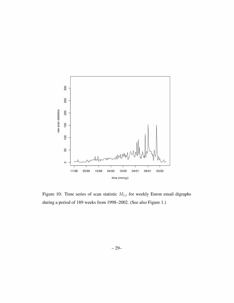
Figure 10: Time series of scan statistic M1,t for weekly Enron email digraphs
during a period of 189 weeks from 1998–2002. (See also Figure 1.)
– 29–

050
100
150
200
250
300
time (mm/yy)
raw
scan
sta
tistic
s
11/98 05/99 10/99 04/00 10/00 04/01 09/01 03/02
Figure 11: Time series of scan statistic M2,t for weekly Enron email digraphs
during a period of 189 weeks from 1998–2002. (See also Figure 1.)
– 30–

050
100
150
time (mm/yy)
stan
dard
ized
scan
sta
tistic
s
11/98 05/99 10/99 04/00 10/00 04/01 09/01 03/02
Figure 12: Time series of standardized scan statistic M0,t for weekly Enron email
digraphs during a period of 189 weeks from 1998–2002. (See also Figure 2.)
– 31–
050
100
150
time (mm/yy)
stan
dard
ized
scan
sta
tistic
s
11/98 05/99 10/99 04/00 10/00 04/01 09/01 03/02
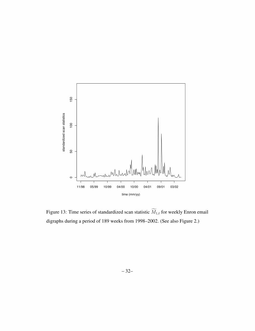
Figure 13: Time series of standardized scan statistic M1,t for weekly Enron email
digraphs during a period of 189 weeks from 1998–2002. (See also Figure 2.)
– 32–

050
100
150
time (mm/yy)
stan
dard
ized
scan
sta
tistic
s
11/98 05/99 10/99 04/00 10/00 04/01 09/01 03/02
Figure 14: Time series of standardized scan statistic M2,t for weekly Enron email
digraphs during a period of 189 weeks from 1998–2002. (See also Figure 2.)
– 33–