Scan Primitives for Vector Computers*

Siddhartha Chatterjee Guy E. Blelloch

School of Computer Science

Carnegie Mellon University

Pittsburgh, PA 15213-3890

Marco Zagha

Abstract

Ibis paper describes an optimized implementation of a set of mm (also called ah-prefix-sums) primitives on a single processor of a CRAY Y-MP, and demonstrates that their use leads to greatly improved performance for several applications that cannot be vectorized with existing compiler technology. The algorithm used to implement the scans is based on an algorithm for par- allel computers and is applicable with minor modifications to any register-based vector computer. On the CRAY Y-MP, the asymptotic running time of the plus-scan is about 2.25 times that of a vector add, and is within 20% of optimal. An important aspect of our implementation is that a set of segmented versions of these scans are only marginally more expensive than the un- segmented versions. These segmented versions can be used to execute a scan on multiple data sets without having to pay the vector startup cost (I) 1,~) for each set.

Routine

plus scan (int)

I r (clks/elt) Scan version 1 Scalar version

2.5 I 7/i(*) segmented plus scan (int)

parallel radix sort (64 bits) branch-sums

root-sums delete-vertices

3.7 74.8 (*j 896.8 11730.0 (*)

12.2 206.5 (t) 9.8 208.6(t)

19.2 276.2 0‘)

Table 1: Incremental processing times per element for primitives and applications discussed in this paper, for both scan and scalar versions. All numbers are for a single processor of a CRAY Y-MP. 1 clock tick = 6 ns. Items marked with (*) were written in Fortran and those marked with (t) were written in C.

The paper describes a radix sorting routine based on the scans that is 13 times faster than a Fortran version and within 20% of a highly optimized library sort routine, three operations on trees that are between 10 and 20 times faster than the corresponding C versions, and a connectionist learning algorithm that is 10 times faster than the corresponding C version for sparse and irregular networks.

create and manipulate more irregular and dynamically varying data structures such as trees and graphs.

1 Introduction

Vector supercomputers have been used to supply the high com- puting power needed for many’ applications. However, the per- formance obtained from these machines critically depends on the ability to produce code that vectorizes well. Two distinct approaches have been taken to meet this goal-vectorization of “dusty decks” [18], and language support for vector intrinsics, as seen in the proposed Fortran 8x standard [ 11. In both cases, the focus of the work has been in speeding up “scientific” com- putations, characterized by regular and static data structures and predominantly regular access patterns within these data struc- tures. These alternatives are not very effective for problems that

Elsewhere, scan (prefix sum) operations have been shown to be extremely powerful primitives in designing parallel algorithms for manipulating such irregular and dynamically changing data structures [3]. This paper shows how the scan operations can also have great benefit for such algorithms on pipelined vector machines. It describes an optimized implementation of the scan primitives on the CRAY Y-MP’, and gives performance numbers for several applications based on the primitives (see Table 1). The approach in the design of these algorithms is similar to that of the Basic Linear Algebra Subprograms (BLAS) developed in the context of linear algebra computations [ 141 in that the algorithms are based on a set of primitives whose implementations are op- timized rather than having a compiler try to vectorize existing code.

‘This research was supported by the Defense Advanced Research Projects Agency (DOD) and monitored by the Avionics Laboratory, Air Force Wright Aeronautical Laboratories, Aeronautical Systems Division (AFSC), Wright- Patterson AFB, Ohio 45433-6543 under Contract J?33615-87-C-1499,ARPA Order No. 4976, Amendment 20.

The remainder of this paper is organized as follows. Section 2 introduces the scan primitives and reviews previous work on vectorizing scans. Section 3 discusses our implementation in detail and presents performance numbers. Section 4 presents other primitives used in this paper, and three applications using these primitives. Finally, future work and conclusions are given in Section 5.=

The views and conclusions contained in this document are those of the ‘CRAY Y-hfP and CF177 arc trademarks of Cray Research, Inc. author and should not be interpreted as representing the official policies, ‘AlI Fortran code discussed in this paper was compiled with CFI77 Ver- either expressed or implied, of DARPA or the U.S. government. sion 3.1. All C code was compiled with Cray PCC Version XMP/YMP 4.1.8.

CH2916-5/90/0000/0666/$01 .OO 0 IEEE 666

2 Scan primitives

A scan primitive takes a binary associative operator +I with left identity I,,,, and a sequence [c/a.. . . , u,,-t] of JI elements, and returns the sequence

[Jo ~ . . . . . I’,,-, ] = [f+,clo.(f/odiol) . . . . . (f!o’P...cfiC/,,-2)].

In this paper, we will only use f and maximum as operators for the scan primitives, as these operators are adequate for all the applications discussed here. We henceforth refer to these scan primitives as f-scan and max-scan respectively. For example:

A = [5 1 3 4 9 21

+-scan(A) = [O 5 6 9 13 221 max-scan(A) = [-,X 5 5 5 5 91

The scan primitives come from APL [lo]. Liver-more loop 11 is a scan with addition as the binary associative operator.

We call the scans as defined above unsegmented scans. Many applications execute the scan operations on multiple data sets. Rather than paying a large startup cost foreach scan, it is desirable to put the sets in adjacent segments of memory and use flags to separate the segments. For example:

A = [5 1 3 4 3 9 21 head-flags = [l 0 0 1 0 1 O]

seg-+-scan(A) = [O 5 6 0 4 0 91

The segmented versions of the scan execute a scan independently on each segment, but only pay the startup cost (II i/z) once. Sec- tion 3.3 discusses the tradeoff, and Section 4.3 gives an example of how they are used.

The uses of both unsegmented and segmented scans are exten- sive. A list of some of them is given below.

1.

2.

3.

4.

5.

6.

7.

8.

9.

10.

To add arbitrary precision numbers. These are numbers that cannot be represented in a single machine word 1171.

To evaluate polynomials [ 191.

To solve recurrences such as .I’, = ~,.r,-i + !I,.,;-z or .I’; = (I( + 1),/.1.,-t (Livermoreloops 6,11, 19 and 23) [12].

To solve tridiagonal linear systems (Livermore Loop 5) [20].

To pack an array so that marked elements are deleted (the PACK intrinsic in Fortran 8x).

To find the location of the first minimum in an array (Liver- more loop 24, and the MINLOC intrinsic in Fortran 8x).

To implement a radix sorting algorithm (see Section 4.1).

To implement a quicksort algorithm [3].

To perform lexical analysis 171.

To implement operations on trees, such as finding the depth of every vertex in a tree (see Section 4.2).

,i’= [[so0 SOI .‘02] [I [.yzo .%I [.‘30 .‘311]

vector elements = [%O .SOI ,-02 ,%O .v21 ,<30 .‘311

head-flags = [I 0 0 1 0 1 O]

lengths = [3 0 2 21

head-pointers = [O 3 3 51

Figure 1: A segmented vector and three ways of describing the segmentation. The head-flags marks the beginning of each segment, the lengths specifies the length of each segment, and the head-pointers points to the beginning of each segment.

11. To label components in two-dimensional images [ 161.

12. To draw a line on a two-dimensional grid given its end- points [4].

13. To solve a variety of graph problems 121.

14. To solve many problems in computational geometry [4].

15. To efficiently implement languages that support nested par- allel structures [5], such as CM-LISP 1231, on flat parallel machines.

Comparison with previous work

There has been significant research on parallel and vector al- gorithms for unsegmented scans. A parallel implementation of scans on a perfect shuffle network was suggested by Stone [ 191 for polynomial evaluation. The problem with this algorithm is that it required O(log ,r) time with O( ,,) processors. Thus it required O(‘t/ log !I) arithmetic operations as opposed to 0( ,,) for the serial algorithm. Stone later showed an optimal ver- sion of the algorithm in the context of solving tridiagonal equa- tions [20]. This algorithm can be implemented in O( log u ) time with 0 (I) / log I) ) processors. When implemented on the CRAY Y-MP, this algorithm results in running times that are longer than those for the algorithm presented in this paper, since it requires intermediate results to be written out to main memory and then read back in again. Other approaches to implementing scans on a vector machine are based on cyclic reduction [8] and unrolling scalar loops [21], which again have larger constant factors than the implementation presented in the paper.

The frequent use of linear recurrences in scientific code has motivated research in finding efficient and vector&able methods for scans. For instance, Livermore loops 5, 6, 11, 19 and 23 involve recurrences that can be expressed in terms of scans. State-of-the-art vectorizing compilers can recognize such linear recurrences and use one of the above algorithms to optimize such loops [15]. However, segmented scans cannot be handled by such techniques. This is the reason that the performance of the unsegmented scalar plus scan in Table 1 is significantly better than that of the segmented plus scan.

667

re z ! 9 : 2, 6 4 8 1 9, 51 processor0 processor 1 PGGZZ processor 3

Sum = [12 7 18 151 +-scan(Sum) = [0 12 19 371

0 4 11 J2 1,2 17, processorO processor 1 j9 2,5 29 processor2 37 3,8 47 processor 3

Figure 2: Executing a scan when there are more elements than processors.

Special hardware support for summation and iteration type operators has been added on some vector machines, the Hitachi S-820 being an example [22]. This machine includes a feedback connection from the output of the ALU to the inputs to support such operations. However, the speed of these instructions is much slower than those of other vector instructions, and efforts to vectorize scans based on such primitives [21] have only been able to realize a very small fraction of the peak performance. The techniques suggested there cannot handle segmented scans either. Our work demonstrates that such specialized hardware is not essential, and that effective use can be made of existing hardware to vectorize scan operations.

Loop interchange [ 181 is a technique used by vectorizing com- pilers to vectorize inner loops by interchanging the order of enclosing loops. It appears that the functionality provided by segmented scans can be achieved through loop interchange tech- niques. This is true for operations on arrays, where the segments (corresponding to rows or columns of the array) are of equal length. However, such techniques would not be applicable to more irregular data structures such as graphs or sparse matrices,

where the segments are not necessarily of the same length. Per- formance there would be dominated by the length of the longest segment. Further, the performance of the loop interchange tech- nique depends on the number of segments and is bad for a small number of segments, whereas the performance of the segmented scan will be shown to be independent of this number.

3 Implementing Scan Primitives

In this section, we present vectorizable algorithms for the un- segmented and segmented scan primitives. We only consider the +-scan, as the algorithms can be easily modified for max-scan by changing the addition operation to a maximum.

We first describe a parallel algorithm for plus-scanning avector of length n on p processors. It has three phases:

1. Processor i sums elements is through (i 3 1 ).q - 1, where s = it //I. (For simplicity assume that n is a multiple of p.) Call this result Sum[i] .

2. The vector Sum is now scanned using a tree-summing [13] or similar algorithm.

?I = (I - 1 ).i + /

Figure 3: Rectangular organization of a vector of length n for scan operations. The vector is fully characterized by specifying the shape factors 1, s andf. Each cell represents one element of the vector. On the CRAY Y-MP, I(0 < I 5 64) is the length of the vector registers used in the computation. s is the stride used to load the vector register from memory, and also the number of iterations of each phase of the algorithm. f is the number of iterations that are executed with a vector register length of 1. The remaining .q - .f iterations are executed with the length set to I- 1.

3. Processor i sums its portion of the vector, starting with Sum[i] as the initial value, and accumulating partial sums. The partial sums are written out to the corresponding loca- tions.

Figure 2 shows an example (the details of the tree-summing step are omitted).

To vectorize the parallel algorithm, consider each element of a vector register as a processor. Then, in the above scheme, element i of the vector register would need to sum elements j-q through (i + 1 )S - 1 of the vector being scanned. This operation can be vectorized by traversing the vector with strides, and using elementwise vector instructions to sum the sections. It is useful to consider the vector (of n elements) as being organized in a rectangular fashion, characterized by three parameters 1, s and f, as shown in Fig. 3. These three parameters characterize the vector completely and are called its shape factors.

Determining the shape factors

From Fig. 3, 11 = (I - 1 ).c + j’. This equation is underspecified for the purposes of determining the shape factors given n. We use the following additional constraints for choosing the parameters:

0 0 < .I’ L: s.

l s is chosen to minimize bank conflicts; it is not allowed to be a multiple of BANKS, a constant that is determined by the number of memory banks and the bank cycle time (4 in the case of the CRAY Y-MP).

l 1 is kept as large as possible, and is upper-bounded by the length of the vector registers (64 in the case of the CRAY Y-MP).

The reason for organizing the data thus is that all memory accesses are now constant-stride, and bank conflicts are avoided.

668

We refer to this method of traversal of the vector as scan order, and the usual unit-stride traversal as index order. Thus, for a vector with I = 4 and H = ./ = 3, a scan order traversal would read the elements in the order ((0, 3, 6, 9), (1,4, 7, lo), (2, 5, 8, 1 l)), whereas an index order traversal would read them in the order NO, 1,2,3), (4,5,6,7), (8,9,10, 11)).

3.1 Algorithm for unsegmented plus-scan

The unsegmented scan algorithm mirrors the parallel algorithm and has three phases. In the following discussion we will assume / = .S for purposes of clarity. If .f < S, the algorithm needs to be modified to decrement the contents of the Vector Length register by 1 for the last (s - j) iterations. This algorithm can be used on any register-based vector machine. In our implementation on the CRAY Y-MP, the loops shown below are unrolled and the registers renamed to avoid locking vector registers. This unrollng speeds up phase 3 by a factor of two.

1. (Phase 1) Elements are summed columnwise, producing 1 sums, thus:

I.-lo = (‘0 + . . . + c’s-l

1-1, = I’, + *. . + I’Z-1

I.1 . = .q,++... I-2 + q/-l)a-I \-1,-l = l’(/-I).s -I- . . . + I’,,-1

The sums I 1; are stored in the elements of a vector reg- ister, which is initialized to zero. The entire computation is vectorizable, as the following C-like pseudo-code shows. In this code, Vl and V2 are vector registers, and the vector length register is set to 1. Vl is used to compute and hold the columnwise sums, and V2 is used to load sections of the source vector.

Vl = 0; k = (l-l) "s; for (i = 0; i < s; i++) {

/* vector fetch with stride s */ V2 = <v[i], v[s+i], . . . . v[k+i]>; Vl = VI + v2; /* vector add */

1

2. (Phase 2) A serial scan is performed on the elements of vector register Vl. After this computation, the new values of the elements are as follows:

I.10 = 0

Src = [2 4 1 1 0 1 -3 2 0 6 1 51

Vector organization = 2 1 -3 6 402 1 1 1 0 5

Vl (in phase 1) =ooo 0 initially 2 1 -3 6 after iter 1 6 1 -1 7 after iter 2 7 2 -1 12 afteriter3

Vl (after phase 2) =079 8

Dst (in phase 3) =079 8 in iter 1 2 8 6 14 in iter 2 6 8 8 15 in iter 3

Dst = [0 2 6 7 8 8 9 6 8 8 14 15

Figure 4: Stages in the execution of the unsegmented scan oper- ation. The diagram shows the organization of the source vector (Src), the intermediate states of Vl during phase 1 of the scan, the values in Vl after phase 2, and the values written out to the destination vector (Dst) during phase 3.

This computation is not vectorized, but is of fixed cost since it only operates on I elements (I 5 64 on the CRAY Y-MP). Moreover, it executes out of the vector register and does not involve any memory transfers.

3. (Phase 3) The elements are again summed columnwise, but using the current values in Vl as an initial offset, as follows:

k = (l-l)*s; for (i = 0; i < s; i++) (

/* vector fetch with stride s */ V2 = <v[i], v[s+i], . . . . v[k+i]>;

/* vector store with stride s */

<d[il, d[s+i], . . ., d[kti]> = Vl; Vl = Vl t v2; /* vector add */

This computation is also vectorizable. The values stored into d are the values resulting from the plus-scan. The vectors d and v can be identical; this does not affect the correctness of the algorithm.

Figure 4 shows the various stage? of the above example, The vector v on which the scan is performed is of length 12, which, for purposes of illustration, is organized with [ = 4 and s = f = 3. It should be noted that the first two phases of the above algorithm can be used to implement a standard reduction (or summation) operation.

669

r,;-, . - . l‘&-l . . . ~~~1-1)9-1 0 ’ O64-1

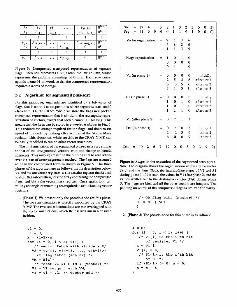
Figure 5: Compressed transposed representation of segment flags. Each cell represents a bit, except the last column, which represents the padding consisting of O-bits. Each row cone- sponds to one 64-bit word, so that the compressed representation requires s words of storage.

3.2 Algorithm for segmented plus-scan

For this primitive, segments are identified by a bit-vector of flags, that is set to 1 at the positions where segments start, and 0 elsewhere. On the CRAY Y-MP, we store the flags in a packed transposed representation that is similar to the rectangular repre- sentation of vectors, except that each element is 1 bit long. This means that the flags can be stored in s words, as shown in Fig. 5. This reduces the storage required for the flags, and doubles the speed of the code by making effective use of the Vector Mask register. This algorithm, while specific to the CRAY Y-MP, can be easily modified to run on other vector machines.

The implementation of the segmented plus-scan is very similar to that of the unsegmented version, with one change to handle segments. This involves resetting the running sum to zero when- ever the start of a new segment is reached. The flags are assumed to be in the compressed form as shown in Figure 5. The three phases of the algorithm are as follows. In the description below, Vl and ~2 are vector registers, Sl is a scalar register that is used to store flag information, F is the array containing the compressed flags, and VM is the vector mask register. Once again, loop un- rolling and register renaming are required to avoid locking vector registers.

1. (Phase 1) We present only the pseudo-code for this phase. The merge operation is directly supported by the CRAY Y-MP. The two scalar instructions can run overlapped with the vector instructions, which themselves run in a chained fashion.

VI. = 0; Sl = 0; k = (1-l)*s; for (i = 0; i < s; it+) {

/* vector fetch with stride s */ V2 = <v[i], v[s+i], . . . . v[kti]>;

/* flag fetch (scalar) */ VM = F[i];

/* reset V1 if F is 1 (vector) */ VI = VI merge 0 with VM; Vl = Vl t ‘i72; /* vector add */

Src = [2 4 1 5 8 1 3 2 3 6 0 5] Seg = [l 0 0 0 0 1 1 0 1 0 0 O]

Vector organization = 2 5 3 6 4 8 2 0 1 1 3 5

Flags organization = 1 0 1 0

0 0 0 0 0 1 1 0

Vl (in phase 1) =o 00 0 initially 2 5 3 6 after iter 1 6 13 5 6 after iter 2 7 1 3 11 after iter 3

Sl (in phase 1) =oooo initially 1 0 1 0 after iter 1 1 0 1 0 after iter 2 1 1 1 0 after iter 3

Vl (after phase 2) =07 13

Dst (in phase 3) =o 7 0 3 initer 1 2 12 3 9 in iter 2 6 0 0 9 in iter 3

Dst = [0 2 6 7 12 0 0 3 0 3 9 91

Figure 6: Stages in the execution of the segmented scan opera- tion. The diagram shows the organizations of the source vector (Src) and the flags (Seg), the intermediate states of Vl and Sl during phase 1 of the scan, the values in Vl after phase 2, and the values written out to the destination vector (Dst) during phase 3. The flags are bits, and all the other vectors are integers. The padding on words of the compressed flags is omitted for clarity.

/* OR flag bits (scalar) */ Sl = Sl 1 VM;

1

2. (Phase 2) The pseudo-code for this phase is as follows:

s = 0;

for (i =

/* v1t of

t = Vl[

0; i < 1; it+) { i] is the i'th elt register V1 */ il;

Vl[i] = 5; /* Sl<i> is the i'th bit

of Sl */ if (Sl<i> != 0) s = 0; 9 = 9 t t;

I

670

This loop runs in scalar mode, but the cost is small and fixed, and it involves no memory transfers.

3. (Phase 3) This phase is similar to phase 1 except that the results are written out and the flags need not be ORed to- gether.

k = (l-l) *s; for (i = 0; i < 5; i++) {

/* vector fetch with stride s */ V2 = <v[i], v[s+i], . . . . v[k+i]>;

/* flag fetch (scalar) */ VM = F[i];

/* reset VI if F is 1 (vector) */ V1 = VI merge 0 with VM;

/* vector put with stride s */

<d[il, d[s+i], . . . . d[k+i]> = Vl; VI = VI + V2;/* vector add */

The packed representation for flags allows successive words to be loaded directly into the Vector Mask register, and a vector merge can be used to reset the values of V. In practice, we cache 64-word sections of the flags in a vector register to cut down on memory access costs.

Figure 6 shows the various stages of the above example. The vector v on which the scan is performed is of length 12, which, for purposes of illustration, is organized with 1 = 4 and s = f = 3. The vector has four segments, of lengths 5, 1, 2, and 4 respectively.

Algorithm for segmented copy-scan

Other useful segmented scan operations include max- and copy- scans. A segmented copy-scan copies values placed at the start- ing positions of segments across the segment, and can be imple- mented in a manner similar to the segmented plus-scan3. The copy-scan copies either the running value or the new value based on the flag at that point, in the same way that the plus-scan ei- ther adds the value to the running sum or clears the sum. The details are similar to the segmented plus-scan and are therefore not repeated here.

3.3 Results

Table 2 presents timing results for our implementations of the scan primitives. We characterize the performance of each oper- ation with two numbers, I, (= l/~,,) and ,,L,z [9], that measure, respectively, the incremental cost of processing one element (in clock cycles), and the vector half-performance length. Our ef- forts have been mostly concerned with reducing I, as this is (asymptotically) the dominant factor in the running time.

The primitives are implemented in Cray Assembler Language (CAL) [6] as a set of routines callable from the C program- ming language. The loops are unrolled twice to avoid register

?his is not a scan as defined in Section 2, but is so called because it can be implemented in a similar manner.

Table 2: 1, (= l/~~.) and H 1,~ values for various scan primitives. The values are for a single processor of a CRAY Y-MP.

reservation effects. Timing measurements were taken with the rtclock ( ) system call, andmultiplemeasurements were taken to smooth out the effects of the presence of other users on the system. A least-squares technique was used to fit a straight line to the points and calculate I, and II 1,~.

Theoretically, I, for both the unsegmented and the seg- mented plus-scan on the CRAY Y-MP for our algorithm is 2 cycles/element, assuming perfect chaining. Our implementation of the unsegmented scan achieves a rate of 2.5 cycles/element, which is 80% of the peak throughput. The segmented scan im- plementation achieves 3.65 cycles/element, 5.5% of the peak rate.

Segmented vs. unsegmented scans

It is clear that the effect of a segmented scan can be simulated by performing an unsegmented scan over each of its segments. We show that this is generally undesirable. Consider a vector of length n containing M segments. The execution time t of a vector operation is given by the following equation [9]:

Using superscripts s and u to indicate, respectively, the seg- mented and unsegmented versions of the scan operation, the times to execute the segmented scan operation by the two meth- ods above are given by:

I’ = I,$( It + //;,2) I, I = I:‘( I? + ttt t02)

The set of unsegmented scans runs faster when:

which, on substituting values from Table 2, gives

/I! < 1.42 $0.0005,,.

This indicates that the unsegmented algorithm should only be used to implement a segmented scan if there are a small number of relatively long segments.

4 Applications

In this section we discuss three applications using these primi- tives: sorting, tree operations, and a connectionist learning algo- rithm called back-propagation. These applications were chosen

1 Eov. Fortran kernels 1 Operation

Elementwise p-add-i(C, A, B, L) p-sub-i(C, A, B, L)

pneg-i (B, A, L) pmax-i (C, A, B, L)

p-inv-i (B, A, L)

extbit(C, A, N, L)

p..sel-i(C, A, B,

F, L)

p-distr..i(A, N, L) Permutation-based

perm-i (C, A, B, L) bperm-i (C, A, B, L) sel-perm-i (C, A, B,

F, L)

C(1) = A(1) + B(1) C(1) = A(1) - B(1) B(1) = -A(I)

IF (A(I) THEN C ELSE C

IF (A(I) THEN B ELSE B

.GT. B(1))

1) = A(1) I) = B(1) .EQ. 0) I) = 1 I) = 0

C(1) = -gbit (A(I), 64-N)

IF (F(1) .EQ. 0) THEN C(1) = A(1) ELSE C(1) = B(1)

A(1) = N

C(B(I)) = AtI) C(I) = A(B(I)) IF (F(I) .EQ. 1)

C(B(I)) = AtI)

Table 3: Other vector primitives used. The kernel loops over the L elements of the vectors. -gbit is an intrinsic function to extract a bit from a word. Some of the kernels cannot be vectorized without a change in the algorithm.

to illustrate the use of the scan primitives in problems that are not regular.

We first introduce a set of primitives in addition to scans that we have implemented as building blocks for applications. These primitives are shown in Table 3 along with their semantics. The elementwise operations correspond directly to elementwise vec- tor instructions found on the Cray. The permutation-based oper- ations are implemented using the gather and scatter instructions. There is obviously a wide variety of operations to choose from in selecting the particular set. The operations we considered primitive were based on considerations of generality and ease of implementation. They were implemented in CAL as the C compiler did not do a good job of vectorizing them.

Table 4 shows the performance of the other primitives, in terms of I, and u 1,~. The performance of the permutation-based operations are data-dependent because of the possibility of mem- ory bank conflicts. We timed identity, reverse and unstructured permutations.

4.1 Sorting

As our first example of the use of the scan primitives, consider a simple radix sorting algorithm. The algorithm is a parallel version of the standard serial radix sort [ 111.

The algorithm loops over the bits of the keys, starting at the lowest bit, executing a split operation on each iteration. The split operation packs the keys with a 0 in the corresponding

Operation 1, “l/2

(clks/elt) (elts)

p-add-i 1.14 483 p-sub-i 1.16 767

P-neg-i 1.11 710 p-max-i 2.12 398 p-inv-i 1.11 700 ext bit 1.11 709 p-Gl-i 2.13 483 p-distr-i 1.09 668 perm-i

(identity) 1.24 663 (reverse) 1.60 499 (unstructured) 1.82 419

bperm-i (identity) 1.56 557 (unstructured) 1.87 446

selgerm i (identity) 3.39 332

Table 4: 1 f (= l/ I’.~, ) and n t ,2 values for other vector primitives. The numbers are for a single processor of a Cray Y-MP.

bit to the bottom of a vector, and packs the keys with a 1 in the bit to the top of the same vector. It maintains the order within both groups. The sort works because each split operation sorts the keys with respect to the current bit (0 down, 1 up) and maintains the sorted order of all the lower bits-remember that we iterate upwards from the least significant bit. Figure 7 shows an example of the sort along with code to implement it.

We now consider how the split operation can be imple- mented using the scan primitives (see Figure 8). The basic idea is to determine a new index for each element and permute the elements to these new indices. This can be done with a pair of scans as follows. We plus-scan the inverse of the Flags into a vector I -down. This gives the correct offset for all the elements with a 0 flag. We now generate the offsets for the elements with a 1 and put them in I-UP, by executing a plus-scan on the flags (we must first add to the initial element the number of 0 elements). We then select the indices from the two vectors I -up and I -down based on the original flags vector. Figure 8 shows our code that implements the split operation. Figure 9 shows a Fortran implementation of the split operation. The available Fortran compiler did not vectorize this code.

The performance of the parallel radix sort on 32- and 64-bit inputs is shown in Table 5. This is within 20% of a highly optimized library sort routine and 13 times faster than a sort written in Fortran.

On the Cray Y-MP, the split operation can be implemented with the compress-index vector instruction with about the same performance (I,) as our implementation. It is interesting that we can get almost the same performance without ever using this instruction which is designed specifically for split type operations.

672

subroutine split(dst, src, fl, len) integer dst(*), src(*), fl(*) integer len

V = [5 7 3 14 21

v(O) = [1 1110 O] V = split(V, V(O}) = [4 2 5 7 3 l]

v(l) = [O 1 0 1 1 O] V = split(V, V(1)) = [4 5 1 2 7 31

VP) =[l 10 0101 V = split(V, V(2j) = [12 3 4 5 71

Figure 7: An example of the split radix sort on a vector contain- ing three bit values. The V(u) notation signifies extracting the t,“’ bit of each element.

p..invb (NotF, Flags, len) ;

plus-scan-i(I_down, NotF, len); /* number of OS in Flags */

sum = NotF[len-l] + I-down[len-11; /* setup correct offset */

Flags[O] += sum; plus-scan-i(I-up, Flags, len);

/* restore flags */ Flags[O] -= sum;

/* fix initial element of I-up */ I-up[O] = sum; p-sel-i(Index, I-up, I-down, Flags, len); perm-i(Result, V, Index, len);

V = [5 7 3 1 4 2 7 21 Flags = [l 1 1 1 0 0 1 01

NotF = [O 0 0 0 1 1 0 l]

I -down = [O 0 0 opJm2 q ] I-UP = [m q q kij 6 6 q 71 Index = [3 4 5 6 0 1 7 21

Result = [4 2 2 5 7 3 1 71

Figure 8: The split operation packs the elements with an 0 in the corresponding flag position to the bottom of a vector, and packs the elements with a 1 to the top of the same vector. All lowercase variables are scalars and all capitalized variables are vectors.

index = 1 do 10 j = 1, len

if (fl(j) .EQ. 0) then dst(index) = src(j) index = index + 1

10 endif

do 20 j = 1, len if (fl(j) .EQ. 1) then

dst(index) = src(j) index = index + 1

20 endif

return end

Figure 9: The split operation implemented in Fortran. The Fortran compilerdidnotvectorizethiscode.

Routine 1, "l/Z (clocks/element) (elements)

spl it operation 10.07 665 Parallel radix sort (32 bits) 421.35 560 Parallel radix sort (64 bits) 896.83 523

Table 5: I,(= l/7.,,) and ~1/2 values for the split operation and the parallel radix sort routine. The numbers are for one processor of a Cray Y-MP.

4.2 Tree algorithms

This section describes three operations on trees:

l branch-sums: given a tree of values, returns to every node the sum of its children;

l root-sums: given a tree of values, returns to every node the sum of the values on the path from the node to the root;

l delete-vertices: givenatree,andaflagateachnode, deletes all the vertices that have a flag set.

Figure 10 illustrates the effects of these operations. Although a serial implementation of the three operations is straightforward, vectorizing these operations is beyond the capability of any vec- torizing compiler. The problem is that there is no way of turning the multiple recursive calls into a loop without introducing a stack to simulate the recursion, and this inhibits vectorization. To vectorize, we have to drastically alter both the representation of a tree and the algorithms used. A description of the repre- sentation and algorithms is beyond the scope of this paper. The interested reader is referred to [2]. The performance numbers

673

Original Tree Branch Sums

Root Sums

Figure 10: Illustration of the tree operations. For the delete vertices the x marks the nodes to be deleted.

for the vector and serial versions of the operations are shown in Table 6.

The trees need not be binary or balanced for these operations. These basic operations can be used to execute the following useful operations on a tree:

l Determining the depth of each vertex. This is executed by applying a root -sums operation on a tree with the value 1 at every vertex.

l Determining how many descendants each vertex has. This is executed by applying a branch-sums operation on a tree with the value 1 at every vertex.

l Passing a flag down from a set of vertices to all their de- scendants. This is executed with an root-sums operation on a tree with a 1 in vertices that want their descendants marked. Any vertex that has a number greater than 0 as a result is marked.

l Passing a flag up from a set of leaves to all their ancestors. This is executed with an branch-sums operation on a tree with a 1 in vertices that want their ancestors marked. Any vertex that has a number greater than 0 as a result is marked.

4.3 A connectionist learning algorithm

As a final example that illustrates the use of the segmented ver- sions of the scan primitives, we examine the forward propa- gation step of a connectionist learning algorithm called back- propagation. Connectionist network models are dynamic sys- tems composed of a large number of simple processing units connected via weighted links, where the state of any unit in the network depends on the states of the units to which this unit connects. The values of the links or connections determine how

Routine 1 Vector Version 1 Scalar Version

1, ‘II/Z I6 ‘)I/2

(clks/elt) (elts) (clks/elt) (elm)

branch-sums 12.2 489 206.5 2 root-sums 9.8 526 208.6 2 delete-vertices 19.2 483 276.2 2

Table 6: I, (= 1 /I,,~.) and I! 1,~ values for the three tree operations. The numbers are for one processor of a Cray Y-ME

one unit affects another. The overall behavior of the system is modified by adjusting the values of these connections through the repeated application of a learning rule.

The back-propagation learning algorithm is an error-correcting learning procedure for multilayered network architectures. In- formation flows forward through the network from an input layer, through intermediate, or hidden layer(s), to an output layer. The value of a unit is determined by first computing the weighted sum of the values of the units connected to this unit and then applying the logistic function, &, to the result. This forward propagation rule is recursively applied to successively determine the unit values for each layer.

Forward propagation consists of four basic steps: distribut- ing the activation values of the units to their respective fan-out weights, multiplying the activations by the weight values, sum- ming these values from the weights into the next layer of units, and applying the logistic function to this value. Although dense matrix algorithms can be used to implement the steps if the net- work was very regular and dense, they will not work efficiently for sparse networks.

Given such a network represented as a directed graph, the for- ward propagation step proceeds as follows. First, the activations of the input units are clamped according to the input text. The algorithm then distributes the activations to the weights using a copy-scan operation, and then all weights multiply their weight by these activations. The result is sent from the output weights to the input weights of the unit in the next layer using a permute. A plus-scan then sums these input values into the next layer of units, and the logistic function is applied to the result at all the unit processors to determine the unit activations. This forward propagation step must be applied once for each layer of links in the network. This set of operations runs at 9.35 cycles/element.

5 Future work and conclusions

This paper has presented efficient implementations of both un- segmented and segmented scan primitives on vector machines, and shown how this leads to greatly improved performance on a representative set of applications. Each of the primitives has almost optimal asymptotic performance, but since they are made available to the application as a library of function calls, we cannot optimize across the primitives. Such optimizations could reduce temporary storage, allocate resources better, and reduce

674

redundant computation; this would make the split operation run twice as fast. We are working on compiler technology to address these issues. We are also looking at using multiple processors on the CRAY Y-MP to speed up the primitives themselves.

The demonstrated speeds of the primitives, and the prospect of even higher throughputs through the methods mentioned above, strongly argue for their inclusion in commonly-available pro- gramming libraries and languages. We believe that such scan primitives (including the segmented versions) should be easily accessible from and included in languages that support vector intrinsics (such as the new Fortran 8x specification). We hope that the ideas presented here will suggest new data structures and algorithmic techniques that will allow vector supercomputers to be used effectively on a much larger variety of problems.

References

r11

PI

[31

r41

VI

161

171

r91

American National Standards Institute. American National Standardfor Information Systems Programming Language Fortran: S8(X3.9-198x), March 1989.

Guy E. Blelloch. Scans as Primitive Parallel Operations. IEEE Transactions on Computers, C-38(1 1):1526-1538, November 1989.

Guy E. Blelloch. Vector Models for Data-Parallel Com- puting. MIT Press, Cambridge, MA, 1990.

Guy E. Blelloch and James J. Little. Parallel Solutions to Geometric Problems on the Scan Model of Computation. In Proceedings International Conference on Parallel Pro- cessing, pages Vo13: 218-222, August 1988.

Guy E. Blelloch and Gary W. Sabot. Compiling Collection- Oriented Languages onto Massively Parallel Computers. Journal of Parallel and Distributed Computing, 8(2), February 1990.

Cray ResearchInc., MendotaHeights, Minnesota. Symbolic Machine Instructions Reference Manual SR-0085B, March 1988.

W. Daniel Hillis and Guy L. Steele Jr. Data Parallel Al- gorithms. Communications of the ACM, 29(12), December 1986.

R, W, Hackney. A Fast Direct Solution of Poisson’s Equa- tion Using Fourier Analysis. Journal of the Association for Computing Machinery, 12(1):95-l 13, January 1965.

R. W. Hackney and C. R. Jesshope. Parallel Computers: Architecture, Programming, and Algorithms. A. Hilger, Philadelphia, PA, Second Edition, 1988.

1101 Kenneth E. Iverson. A Programming Language. Wiley, New York, 1962.

[l l] D. E. Knuth. Sorting and Searching. Addison-Wesley, Reading, MA, 1973.

Cl21

[131

1141

[la

i361

1171

[181

WI

c201

PII

E221

WI

Peter M. Kogge and Harold S. Stone. A Parallel Algo- rithm for the Efficient Solution of a General Class of Re- currence Equations. IEEE Transactions on Computers, C- 22(8):78&793, August 1973.

Richard E. Ladner and Michaei J. Fischer. Parallel Prefix

Computation. Journal of the Association for Computing Machinery, 27(4):831-838, October 1980.

C. L. Lawson, R. J. Hanson, D. R. Kincaid, and F. T. Krogh. Basic Linear Algebra Subprograms for Fortran Usage. ACM Transactions on Mathematical Software, 5(3):308-323, September 1979.

John M. Levesque and Joel W. Williamson. A Guidebook to Fortran on Supercomputers. Academic Press, Inc., San Diego, CA, 1989.

James J. Little, Guy E. Blelloch, and Todd A. Cass. Algo- rithmic Techniques for Computer Vision on a Fine-Grained Parallel Machine. IEEE Transactions on Pattern Analysis and Machine Intelligence, 11(3):244-257, March 1989.

Yu. Ofman. On the Algorithmic Complexity of Discrete Functions. Soviet Physics Doklady, 7(7):589-591, January 1963.

Constantine D. Polychronopoulos. Parallel Programming and Compilers. Kluwer Academic Publishers, Norwell, MA, 1988.

Harold S. Stone. Parallel Processsing with the Perfect Shuf- fle. IEEE Transactions on Computers, C-20(2): 153-161, 1971.

Harold S. Stone. Parallel Tridiagonal Equation Solvers. ACM Transactions on Mathematical Software, 1(4):289- 307, December 1975.

Y. Tanaka, K. Iwasawa, S. Gotoo, and Y. Umetani. Com- piling Techniques for First-Order Linear Recurrences on a Vector Computer. In Proceedings Supercomputing ‘88, pages 174-l 8 1, Orlando, Florida, November 1988.

Hideo Wada, Koichi I&iii, Masakazu Fukagawa, Hiroshi Murayama, and Shun Kawabe. High-speed Processing Schemes for Summation Type and Iteration Type Vector Instructions on HITACHI Supercomputer S-820 System. In Proceedings 1988 ACM Conference on Supercomput- ing, pages 197-206, July 1988.

Skef Wholey and Guy L. Steele Jr. Connection Machine Lisp: A Dialect of Common Lisp for DataParallel Program- ming. In Proceedings Second International Conference on Supercomputing, May 1987.

675