8

Scam Light Field Rendering

Jingyi Yu and Leonard McMillan

NE43-256, 545 Technology Square, Cambridge, Massachusetts 02139, USA jingyi@graphics.lcs.mit.edu

mcmillan@graphics.lcs.mit.edu

Steven Gortler

Division of Engineering and Applied Sciences, Harvard University,

Cambridge, Massachusetts 02139, USA sjg@deas.harvard.edu

In this article we present a new variant of the light field representation that supports

improved image reconstruction by accommodating sparse correspondence information.

This places our representation somewhere between a pure, two-plane parameterized, light

field and a lumigraph representation, with its continuous geometric proxy. Our approach

factors the rays of a light field into one of two separate classes. All rays consistent with a

given correspondence are implicitly represented using a new auxiliary data structure,

which we call a surface camera, or scam. The remaining rays of the light field are

represented using a standard two-plane parameterized light field. We present an efficient

rendering algorithm that combines ray samples from scams with those from the light

field. The resulting image reconstructions are noticeably improved over that of a pure

light field.

Keywords: Light Field; Correspondence; Scam;

1. Introduction

Light fields are simple and versatile scene representations that are widely used for image-

based rendering [13]. In essence, light fields are simply data structures that support the

9

efficient interpolation of the radiance estimates along specified rays. A common

organization for light fields is a two-plane parameterization in which the intersection

coordinates of a desired ray on two given planes determines the set of radiance samples

used to interpolate an estimate. A closely related representation to a light field is the

lumigraph [9]. A lumigraph incorporates an approximate geometric model, or proxy, in

the interpolation process, which significantly improves the quality of the reconstruction.

Unfortunately, every desired ray must intersect some point on the geometric proxy in

order to estimate its radiance in a lumigraph. Thus, a continuous, albeit approximate,

scene model is required for lumigraph rendering. Acquiring an adequate scene model for

lumigraph rendering can be difficult in practice. In fact, most lumigraphs have been

limited to scenes composed of a single object or a small cluster of scene elements. The

geometric scene proxy used by a lumigraph can be created using computer vision

methods or with a 3-D digitizer. Geometric information about the scene is important for

eliminating various reconstruction artifacts that are due to undersampling in light fields.

An analysis of the relationship between image sampling density and geometric fidelity

was presented by [4]. Chai, et al, presented a formal bound on the accuracy with which a

geometric proxy must match the actual geometry of the observed scene in order to

eliminate aliasing artifacts in the image reconstruction. As with the lumigraph model they

assume that a geometric proxy can be identified for any requested ray.

Acquiring dense geometric models of a scene has proven to be a difficult computer

vision problem. This is particularly the case for complicated scenes with multiple objects,

objects with complicated occlusion boundaries, objects made of highly reflective or

transparent materials, and scenes with large regions free of detectable textures or shading

variations. The wide range of depth extraction methods that have been developed over the

past 40 years, with the objective of extracting geometric models, have met with only

limited success. Even with the recent development of outward-looking range scanners it

is still difficult to create a dense scene model. However, both passive stereo and active

range scanners are usually able to establish the depth or correspondence of a sparse set of

scene points with a reasonably high confidence. The primary objective of this research is

to incorporate such sparse geometric knowledge into a light field reconstruction

algorithm in an effort to improve the reconstruction of interpolated images.

10

Our light field representation factors out those radiance samples from a light field

where correspondence or depth information can be ascertained. We introduce a new data

structure that collects all of those rays from a light field that are directly and indirectly

associated with a 3D point correspondence. This data structure stores all of the light field

rays through a given 3D point, and, therefore, it is similar to a pinhole camera anchored

at the given correspondence. Since this virtual pinhole camera is most often located at a

surface point in the scene, we call it a surface camera, or scam for short. Once the rays

associated with a scam are determined, they can be removed from the light field. We call

this partitioning of rays into scams a factoring of the light field. Ideally, every ray in a

light field would be associated with some scam, and, thus, we would call it fully factored.

The resulting scam light field would generate reconstructions comparable to those of a

lumigraph, although the two representations would be quite different. The utility of a

scam renderer lies in its ability to improve light field reconstructions with a set of scams

that are a small subset of a fully factored light field and do not require to be accurate.

In this article, we describe a new light field representation composed of a collection

of implicit scam data structures, which are established by sparse correspondence

information, and an associated light field, which is used to interpolate rays for those parts

of the scene where no scam information has been established. We describe how to factor

all of the rays associated with a specified scam from a light field when given as few as

two rays from the scam (i.e. a correspondence) or the depth of a single known point. We

then describe the necessary bookkeeping required to maintain the scams and light field

representations. Next we describe an efficient two-pass rendering algorithm that

incorporates scam information, and thus, sparse correspondence information, to improve

light field reconstructions. Finally, we show results of light field renderings using our

new representation with varying degrees of geometric sparseness

2. Background and Previous Work

11

Figure 1: light field rendering: system setup and rendering algorithm: (a) Conventional light field uses an array of cameras uniformly positioned on a plane [22]; (b) Light field assumes constant scene depth and it renders a new ray by intersecting the ray with the focal plane and back-traces and blends its closest neighboring rays.

In recent years, image-based modeling and rendering (IBMR) has become a popular

alternative to conventional geometry-based computer graphics. In IBMR, a collection of

reference images are used as the primary scene representation [9][14]. Early IBMR

systems such as 3D warping [17], view interpolation [5] and layered-depth images [19],

etc, rely heavily on the correctness of depth approximations from stereo algorithms.

Previous work in IBMR has further shown that the quality of the resulting synthesized

images depends on complicated interactions between the parameterization of the given

ray space [10][14], the underlying sampling rate [4][14] and the availability of

approximate depth information [2][9].

Light field rendering is a special form of image-based rendering. It synthesizes new

views by interpolating a set of sampled images without associated depth information.

Light field rendering relies on a collection of densely sampled irradiance measurements

along rays, and require little or no geometric information about the described scene.

Usually, these measurements are acquired using a series of pinhole camera images

acquired along the surface of a parameterized, two-dimensional, manifold, most often on

a plane as is shown in Figure 1(a).

12

Figure 2: Light field rending algorithm: (a) assumes the scene lies at infinity; (b) assumes the scene lies at the optimal focal plane; (c) uses prefiltering on (a); (d) uses prefitering on (b); (e) uses dynamically reparameterized light field(DRLF) and puts the focal plane on the red stuffed animal with a large aperture; (f) uses DRLF and puts the focal plane on the guitar with large aperture.

13

Standard light field assumes constant scene depth, which is called the focal plane. To

render a new ray r, it first interests r with the focal plane. Then it collects the closest rays

to r that passes through the camera and the intersection point. Finally light field rendering

interpolates or blends r from these neighboring rays, shown in Figure 1(b). In practice,

simple linear interpolation method like bilinear interpolation is used to blend the rays.

When undersampled, the light field rendering exhibits aliasing artifacts, as is shown in

Figure 2(a). Levoy and Hanrahan [14] suggested that light field aliasing could be

eliminated with proper prefiltering. Prefiltering can be accomplished optically by using a

camera whose aperture is at least as large as the spacing between cameras. Otherwise,

prefiltering can be accomplished computationally by initially oversampling along the

camera-spacing dimensions and then applying a discrete low-pass filter, which models a

synthetic aperture. In practice, it is usually impractical to do oversampling since it

requires cameras be positioned very close to each other or have large aperture. The other

major issue is the large storage requirement since dense sampling means a tremendously

large number of images. Therefore the only practical way to reducing aliasing in

conventional light field is to use band-limited filtering, i.e., low pass filtering. However,

low-pass filtering has the side effects of removing high frequencies like sharp edges and

view-dependencies, and will incur undesirable blurriness in reconstructed images, as is

shown in Figure 2(c).

A special prefiltering technique to remove aliasing is the dynamic reparameterized

light field [12]. The dynamic reparameterized light field techniques synthesize virtual

aperture and virtual focus to allow for any particular scene element (depth) to be

reconstructed without aliasing artifact. However only those scene elements near the

assigned focal depth are clearly reconstructed and all other scene elements are blurred, as

is shown in Figure 2(e) and 2(f). This kind of prefiltering hence has the undesirable side

effect of forcing an a priori decision as to what parts of the scene can be clearly rendered

thereafter. The introduction of clear and blurry regions of focus in a prefiltered light field

is a direct result of the depth-of-field effects seen by a finite (non-pinhole) aperture. In

addition, view dependencies like specular high lights will be reduced or even removed

because such features are usually not presented in all data cameras or do not have

consistent focal depth.

14

Plenoptic sampling [4] analyzed the relationship between the sample rate and the

geometrical information. Plenoptic sampling also suggested that one can minimize the

aliasing artifacts by placing the object or focal plane at a distance from the camera plane

that is consistent with the scene’s the average disparity, as shown in Figure 2(b). When

the light field is undersampled, it still exhibits aliasing artifacts and using prefiltering

incurs undesirable blurriness shown in Figure 2(d). Lumigraph rendering [9] addresses

the issue of sparse sampling by introducing geometric information and showed that the

rendering quality is significantly improved with approximate geometry proxies even in a

sparsely sampled light field. Our work assumes that it is difficult to provide dense

sampled geometric proxies, or dense correspondences. We design an algorithm to render

views using a sparse set of correspondences and a sparsely sampled light field.

Rendering new views from a set of images have also been studied in the computer

vision community. Shape-from-image techniques, such as shape-from-shading [11] have

long been studied and its major goal is to reconstruct the 3D geometry of the scene from

one or more images. These methods usually work for single and simple objects with

specific surface models and are not suitable to reconstructing real scenes with

complicated occlusions and surface properties. An alternative is to model such scenes as

3D points with depths that are usually stored implicitly in the form of correspondences.

Lots of researches have focused on robust correspondence generation algorithms. Most of

these algorithms, like graph-cut/maximum flow method [2] and the dynamic

programming algorithms [8] are successful on textured Lambertian surfaces but exhibit

poor performance on non-textured regions, surface regions with view-dependent

reflection, and occlusion boundaries. These conditions lead to inaccurate

correspondences for most computer vision algorithms, and hence incorrect geometry

reconstruction and problematic rendering. Recent studies [13][15] in computer vision

focus on segmenting occlusion boundaries and modeling specular highlight from densely

sampled images. These methods usually require dense sampling and high computation

cost that are not suitable for real-time light field rendering.

Our approach first factors all of the rays associated with the constraint plane of each

correspondence using a special data structure called “surface camera” or scam. We assign

a weight to each scam according to its quality and associated disparity. When rendering,

15

we blend them with their weights by a similar algorithm like the unstructured lumigraph.

We will show that our algorithm successfully renders occlusions and view-dependencies

even though the correspondences of those regions are inaccurate. For desired rays that are

not interpolated by any scam, we use the light field approach to render them. In addition,

we present an interactive rendering system that allows users to specify or remove

correspondences and re-renders the view in real-time. Figure 13 and 14 illustrates the

various rendering results using scam-rendering algorithm with correspondence from

multiple objects.

3. Scam Parameterization

In conventional light fields, a two parallel plane parameterization is commonly used to

represent rays, where each ray is parameterized in the coordinates of the camera plane

(s, t) and an image plane (u, v). Surface light fields [21] suggested an alternative ray

parameterization where rays are parameterized over the surface of a pre-scanned

geometry model. We combine both parameterizations in our algorithm.

For simplicity, we assume uniform sampling of the light field and use the same

camera settings as Gu et al [10], where the image plane lies at z = -1 and the camera

plane lies at z = 0, as is shown in Figure 3. This leads to the parameterization of all rays

passing through point (px,, py, pz) as

)1()/11,0,1,0(ˆ)0,/11,0,1(ˆ

)/,/,0,0()ˆ,ˆ,ˆ,ˆ(ˆ

zz

zyzx

ptps

ppppvuts

+⋅++⋅+

−−=r

We use a slightly different parameterization of [9]; we parameterize each ray as the 4-

tuple (s, t, u, v), where (u, v) is the pixel coordinate in camera (s, t). This parameterization

is more natural and gives a simple ray parameterization as

)2()/1,0,1,0()0,/1,0,1(

)/,/,0,0(

)ˆˆ,ˆˆ,ˆ,ˆ(ˆ),,,(

zz

zyzx

ptps

pppp

tvsutsvuts

⋅+⋅+

−−=

−−= rr

16

Figure 3: Correspondence parameterization: each correspondence is identified by two rays from the light field and because they both pass the same 3D point in space, each correspondence forms two similar triangles and the ratio represents the disparity of the correspondence. Notice the red ray that passes through the 3D point and (0, 0) on s-t plane intersects u-v plane at (u0, v0).

The ray-point equations (1) and (2) indicate that all rays passing through the same 3D

point lie on an s-t plane in the 4D ray space, which we call the point’s constraint plane.

In a calibrated setting, each correspondence identifies a unique 3D point; therefore, it

also identifies a constraint plane. Our goal is to first factor all of the rays associated with

the constraint plane of each correspondence using a special data structure called “surface

camera” or scam. We then suggest an algorithm that synthesizes new views from these

scams using a reconstruction algorithm similar to the rebinning approach described for

unstructured cameras in the lumigraph. For desired rays that are not interpolated by any

scam, we use the light field approach to render them. In addition, we present an

17

interactive rendering system that allows users to provide or remove correspondences and

re-renders the view in real-time.

.

3. Scam factoring Correspondences can always be specified as scalar disparities along epipolar lines. We

will assume that all source mages have to be rectified such that their epipolar planes lie

along pixel rows and columns. In this setting disparities can be describe the horizontal

and/or the vertical shifts between the corresponding pixels of image pairs, as is shown in

Figure 2. Each correspondence is represented as two rays ),,,( 11111 vutsr and

),,,( 22222 vutsr , which pass through the same 3D point. Assuming uniform sampling,

and applying the constraint plane equation (2), we have

dispptt

vvssuu

z

==−−

=−− 1

12

12

12

12 (3)

where disp is the disparity of a correspondence. We can rewrite the point’s constraint

plane equation (2) in terms of its disparity as

)4(),0,1,0()0,,0,1(),,0,0(),,,( 00

disptdispsvuvuts

⋅+⋅+=r

This construction transforms each correspondence into a constraint plane defining a set

of 4-dimensional rays. The values of u0 and v0 can be determined directly from the

correspondence rays, r1 and r2. All other rays can be factored from the given light field by

setting the values of s and t and solving for the appropriate u and v values consistent with

the constraint plane of the correspondence. The constraint plane solutions at integer

values of s and t are equivalent to placing a virtual camera at the 3D point and computing

rays from that point through the camera centers lying on the camera plane, as is shown in

Figure 4(a). We implicitly store constraint plane as an image parameterized over the same

domain as the camera plane. We call this image a “surface camera” or scam. To index the

rays of a scam, we solve the disparity equation (4) for all data camera locations shown in

18

Figure 4: Factoring scam: (a) a correspondence is specified as two points and can be factored to all cameras by back projection the 3D point; (b) by normalizing the a correspondence with unit disparity, we can factoring all rays associated with a scam.

Figure 4(b). Because these rays do not necessarily pass through the pixels (samples) of

the data cameras, we bilinearly interpolate their color in the data image. The complete

factoring algorithm is shown as follows:

Generate scam for each correspondence for each correspondence S do

normalize S in form (u0 , v0 , disp) for each data camera C(s, t) do

calculate the projection (u, v) of S in camera C(s, t) from the disparity equation (4) bilinearly interpolate P(u, v) in C(s, t) store P as pixel (s, t) in scams

end for end for

4. Scam Representation

19

All rays passing through a correspondence should all lie on its constraint plane and scam

image and therefore it is important to correctly interpolate the scam image to render new

rays. When a correspondence is accurate, i.e., its corresponding 3D point lies close to the

real surface and is not occluded in any camera view, its scam image reflects the radiance

properties of this point on the surface. For most surfaces, their radiance functions are

smooth and have small variance. Similar to reconstructing 2D signals from samples,

simple interpolation method like bilinear interpolation is sufficient. If a scam is on the

view-dependent spots, it then exhibits variation in intensity. In that case, better

reconstruction filters that preserves high frequencies is more appropriate. Furthermore,

when a scam is on occlusion boundaries, it exhibits sharp transitions between occluded

and non-occluded rays and edge-preserving filters is the correct choice to interpolate the

image.

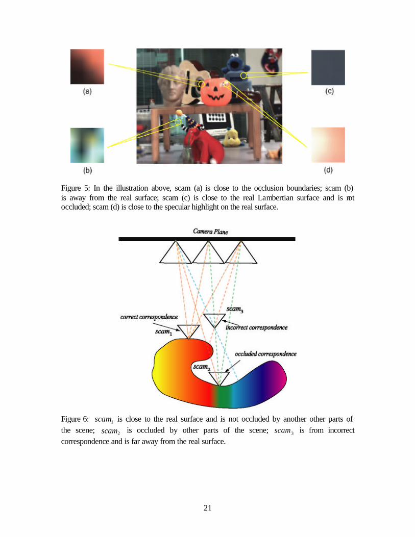
The scam image of a correspondence close to the real surface indicates the radiance

received at all data cameras and thereby represents the surface’s local reflectance

radiance, shown as scam1 of Figure 6. Moreover, if the surface is Lambertian, then these

scams are expected to have constant color everywhere, as is shown in Figure 5(c). If the

surface’s reflectance exhibits view dependencies such as specular highlights, we expect

to observe smooth radiance variations over the scam images. Figure 5(d) shows the scam

of the specular highlight on the pumpkin. Finally, if a correspondence is not close to the

real surface, then we expect to observe greater variations in its scam images, as shown in

scam3 of Figure 6 and Figure 5(b).

When a correspondence lies close to the occlusion boundary of an object, then we

expect to see specific abrupt color transitions in its scam image. Rays that are not

occluded should have consistent colors, while occluded rays might exhibit significant

color variations and discontinuities, as shown in scam2 of Figure 6 and Figure 5(a). Since

we bilinearly interpolate each scam image, we model the scene with “smooth occlusion”

by implicitly interpolating between points on either side of the occlusion boundaries.

Because correspondences are usually not very accurate, we can further estimate a

measure of the quality of correspondences by calculating the distribution and the variance

of the colors within scams. The color distribution in incorrect correspondences should be

discontinuous, non-compact, and its variance is expected to be high. For the correct

20

correspondences and unoccluded surfaces, we expect to see more uniform and continuous

color variations, and, therefore, low color variance. For correspondences on simple

occlusion boundaries, we can characterize them by modeling bimodal color distributions

from their scam images using the method described. And for view-dependent spots like

specular highlights, we model them as combinations of Gaussian functions.

The quality of the scam depends on its accuracy, occlusion condition and view

dependencies. An accurate correspondence on non-occluded Lambertian surface should

have uniform color in within its scam image. Correspondences on occlusion boundaries

should have partial consistencies as well as sharp changes within their scam images.

Accurate correspondences on view-dependent spots like specular highlights have a

Gaussian-like smooth distribution. And inaccurate correspondences are expected to have

random colors within their scam images.

We can therefore measure the quality of the scam as following; we first calculate the

variance of the color in the scam image. If the variance is below certain threshold, then

we assume the scam is on the non-occluded Lambertian surface and we assign a large

weight to the scam; otherwise we estimate if there is abrupt changes in the image, if so,

we fit a bimodal distribution to it and classify it as occlusion boundaries. Otherwise, we

fit a 2D Gaussian function to the scam and classify it as a view-dependent scam. If the

fitting error is small, we then treat the scam as on occlusion boundaries or on a non-

Lambertian surface and assign the weight according the fitting error. Otherwise, we

assume the scam is incorrect and assign a small weight or simply discard it. Moreover,

we assign different interpolation methods in respect to their type. The complete scam

classification algorithm is as follows:

21

Figure 5: In the illustration above, scam (a) is close to the occlusion boundaries; scam (b) is away from the real surface; scam (c) is close to the real Lambertian surface and is not occluded; scam (d) is close to the specular highlight on the real surface.

Figure 6: 1scam is close to the real surface and is not occluded by another other parts of the scene; 2scam is occluded by other parts of the scene; 3scam is from incorrect correspondence and is far away from the real surface.

22

Classify scams: for each scam S do

calculate the color variance var of S if var colorflatthreshold _<

maxmetricmetricquality = RENDER_METHOD = BI_LINEAR end if else do if S has abrupt color changes

fit a bimodel function to S in term of least square error err if boundarythresholderr <

)exp(max errmetricmetricquality −⋅= RENDER_METHOD = EDGE_PRESERVE end if else do minmetricmetricquality = or discard the scam end else end else else fit a 2D Gaussian function to S in term of least square error err )exp(max errmetricmetricquality −⋅= RENDER_METHOD = BI_CUBIC end else end else

end for

5. Scam Rendering

In order to render a correspondence from an arbitrary view, we need to first project its

scam onto the desired view. We do this by constructing a ray from the desired view that

is consistent with the correspondence. We then use the scam data structure to interpolate

the reflected radiance. The explicit coordinates of the 3D point are not needed to

construct the ray. We can instead compute the intersection of the correspondence’s

constraint plane with the camera’s image plane. This is particularly efficient with our

representation.

23

5.1. Projecting correspondences

We describe all virtual cameras in form (s’, t’, z’), where z’ is the distance to the data

camera plane. If the camera is on the camera plane, i.e., at (s’, t’, 0), we can calculate the

projection of the correspondence in the new view using the disparity equation (4) as

)','(),( 00 disptvdispsuvu ⋅+⋅+= (5)

And we can query the color of the projected correspondence by interpolating point (s, t)

in its scam image. To determine the projection of a correspondence in a camera (s’, t’, z’)

off the camera plane, we first calculate its projection (u, v) in camera C’(s’, t’, 0).

Because C’ is on the camera plane, we can simply calculate (u, v) as (5).

We then apply the geometry relationship as is shown in Figure 7(a) and use the depth-

disparity equation (3), we have

dispzzz

zzDzzD

vv

uu

⋅+=

+=

+==

'11

'/)'/(''

(6)

Therefore the projection of the correspondence in the new camera (s’, t’, z’) can be

computed as

)7())'1(/)'(,)'1(/)'(()','(

0

0

dispzdisptvdispzdispsuvu

⋅+⋅+⋅+⋅+=

We then calculate the intersection point (s”, t”, 0) of the ray with the original camera

plane. Notice the correspondence should project to the same pixel coordinates in both

camera (s’, t’, z’) and (s”, t”, 0), as is shown in Figure 7(b). Therefore by reusing

disparity equation (4), we can calculate (s”, t”) as

)8())'1(/)''(,)'1(/)''((

))/)'(,/)'(()'',''(

0

0

00

dispzvztdispzuzs

dispvvdispuuts

⋅+⋅−⋅+⋅−=−−=

The color of the projected correspondence is then bilinear interpolated at (s”, t”) in the

scam image of the correspondence.

24

Figure 7: Projecting the correspondence in the new view: (a) we project the correspondence onto camera (s’, t’, z’) by first projecting it onto camera (s’, t’, 0) and then calculating its projection with geometric relationships; (b) we construct the ray that passes the correspondence from camera (s’, t’, z’) by computing its intersection (s”, t”, 0) with the original camera plane and interpolating it from the scam.

25

5.2. Color blending

Once we project all correspondences onto the new camera, we need to synthesize the

image from these scattered projection points. We use a color-blending algorithm similar

to unstructured lumigraph [2]. We assume correspondences are comparatively accurate

and therefore its projection only influences a limited range of pixels around it in the new

view. In practice, we only blend correspondences projected in a pixel’s 1-ring

neighborhood. If there isn’t any, we then render the pixel directly from the light field. We

use the following weight function to blend these correspondences:

)9()()(

)()(

tan

icorrespmetricicorrespmetric

iscammetricicorrespweight

disparity

cedis

smoothness

++=

The first term of the weight evaluates the quality of the scam, where we use the color

variance as a simple measurement, as is discussed in Section 4. The second term

measures how close the projection is to the pixel, where closer projections get higher

weight. The last term distinguishes closer correspondences from far away ones by their

disparities. For a boundary pixel, there could be multiple correspondences with difference

disparities around it. Since closer objects are expected to be more important, we assign

larger weight to those of large disparities. Furthermore, we assign continuous metric

functions for all terms to maintain the smooth transition from scam rendered parts to light

field rendered parts. The complete two-pass rendering algorithm is shown as follows:

Synthesize view C(s’, t’, z’) for each correspondence S do

calculate ray r(s”, t”) that passes S and C(s’, t’, z’) using equation (8) interpolate r in the scam image of S

calculate the projection P(u’, v’) of S in C using equation (7) compute the weight of S using equation (9) and add S to P’s 1-ring pixels’ scam list

end for for each pixel P(u, v) in the synthesized image do if P’s scam list is not empty do

color blend all correspondences in P’s scam list with calculated weights end if

26

else do use light field to render P end else end for

6. Scam Generation

To generate correspondences, we start with correlating regions from a pair of images that

users can provide with our interactive tools. We then generate correspondences by

sweeping through scanlines between the two regions under epipolar constraints. The

epipolar constraints guarantee that two rays associated with each correspondence

intersect at a 3D point in object space.

Furthermore we assume two additional constraints:

• Ordering constraint: corresponding points appear in the same order along epipolar

lines.

• Piecewise continuity: 3D geometries are piecewise continuous.

Notice the ordering constraint is not always valid, especially for regions close to

occlusion boundaries. It, however, prohibits intercrossing between correspondences and

allows us to use a large class of dynamic programming based algorithms to generate

correspondences. In addition, as is mentioned in previous chapters, our rendering

algorithm does not heavily rely on the accuracy of the correspondences for rendering

quality since low quality correspondences will be “overwritten” by high quality ones in

our quality-biased blending schemes. Piecewise continuity constraint assumes the 3D

geometry is continuous, e.g., occlusion boundaries are continuous. This matches well

with the continuity assumption in our scam-rendering algorithm where we implicitly

maintain a continuous light field. We will discuss in details this continuous light field

property later this chapters.

Given two regions from two images, our goal is to first determine pairs of scanlines to

be correlated to generate correspondences. Recall the ray-point parameterization as

)3(),0,1,0()0,,0,1(

),,0,0( 00

disptdisps

vu

⋅+⋅+=r

27

Obviously, if the two images are on the same row or column, i.e., have the same t or s

coordinates, then the two rays of each correspondence should lie on the same horizontal

or vertical scanline as well. In general, two rays ),,,( 1111 vutsr and ),,,( 2222 vutsr of a

correspondence between images ),( 11 ts and ),( 22 ts must satisfy

)10()()(

21

21

2010

2010

21

21

ttss

disptvdisptvdispsudispsu

vvuu

−−

=⋅+−⋅+⋅+−⋅+

=−−

In other words, the scanlines to be correlated between the two regions should have the

same slope, i.e., the slope of the two images in image space.

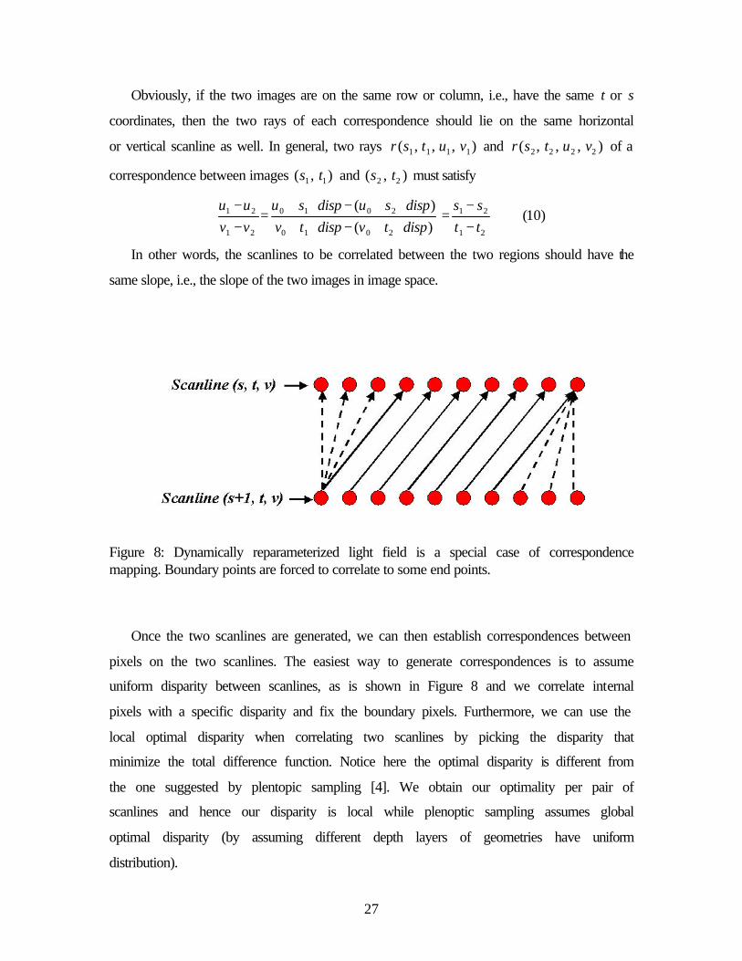
Figure 8: Dynamically reparameterized light field is a special case of correspondence mapping. Boundary points are forced to correlate to some end points.

Once the two scanlines are generated, we can then establish correspondences between

pixels on the two scanlines. The easiest way to generate correspondences is to assume

uniform disparity between scanlines, as is shown in Figure 8 and we correlate internal

pixels with a specific disparity and fix the boundary pixels. Furthermore, we can use the

local optimal disparity when correlating two scanlines by picking the disparity that

minimize the total difference function. Notice here the optimal disparity is different from

the one suggested by plentopic sampling [4]. We obtain our optimality per pair of

scanlines and hence our disparity is local while plenoptic sampling assumes global

optimal disparity (by assuming different depth layers of geometries have uniform

distribution).

28

To obtain better quality scams, we assume the ordering constraint so that we are able

to use a large class of dynamic programming algorithms from computer vision research.

The basic idea of these dynamic programming-based methods is to transform the problem

of finding correspondences into finding the optimal path in a directed graph. For

example, to correlate two scanlines with m and n pixels, we first form an mxn correlation

graph where each node (i, j) in the graph represents the similarity between pixel i and j in

its corresponding scanlines. And we can find a best sequence of correspondences

between these two scanlines by finding the path from node (0, 0) to node (m, n) with

highest overall correlation scores. The ordering constraint guarantees that the correlation

graph is directional and hence we may apply dynamic programming algorithms to find

these optimal paths as is shown in Figure 9.

We start with calculating the correlation correl(i, j) between pixel i in the first

scanline and j in the second. Ideally, we need the linear invariance despite the changes in

illumination. This linear invariance property can be easily achieved by using CIE model

with xyY color space. x and y are good indicators of the actual color, regardless of the

luminance. We nevertheless have to deal with a new non-linearity in the transform

between RGB and CIE xyY. In a light field where illumination remains almost constant

for all images, simple RGB color distance also works well in practice. We further assume

the minimum depth of the scene as the largest disparity as maxdisp and assign the weight

of each node in the graph as:

)11(;)()()(2553

;2553),( 2222

max2

−−−−−−×+>>×

=otherwisebbggrr

dispjiorijifjicorrel

jijiji

Denote Opt(i, j) as the optimal path that that goes from (0, 0) through (i, j); then we

deduce the dynamic programming equation as:

)12(),1(),()1,(),(

max),(

−+−+

=jiOptjicorrel

jiOptjicorreljiOpt

A routine dynamic programming method solves this problem in )( 2NO time and

gives the complete optimal path from (0, 0) to (m, n). Then for each node (i, j) on the

path, we correlate pixel i and j on the two scanlines as a scam. Figure 10 compares the

dynamic programming method and the optimal disparity method by showing the Eipolar

29

Images by interpolating correspondences between scanlines. The optimal disparity

method aligns most of the features correctly except the white/black stripe since its

corresponding geometries is not close to the presumed the optimal focal plane and we

observe serious aliasing artifacts in these regions. The dynamic programming method,

however, manages to remove these aliasings by correctly aligning them.

Figure 9: We can triangulate two scanlines directly from the optimal path of the correlation graph.

The dynamic programming has been used widely in the computer vision field, whose

main goal is to completely reconstruct the 3D surface. Unfortunately it has several major

artifacts. First of all, it adapts poorly to non-textured regions where it is very sensitive to

small noises on uniform-colored surfaces. Second, it cannot handle view-dependencies

such as specular highlights where the correlations are low for points on these surfaces.

Third, the ordering constraints are not always valid for cameras with large baselines

30

where intercrossing may happen. It becomes more problematic on occlusion boundaries

to determine the depth of pixels on these occlusion boundaries.

Fortunately these defects for most stereo algorithms cast much fewer artifacts on our

scam-rendering algorithm. Recall that our scam-factoring algorithm distribute each

correspondence into the light field and then measure its quality in its scam image,

therefore inaccurate correspondences are given much lower priorities when rendering. As

a result, it will be “overwritten” by its good neighbor scams ones and hence has much

fewer artifacts. Furthermore, on the occlusion boundaries where most computer vision

algorithms fail to reconstruct accurate geometries, our scam-rendering algorithm

smoothly blends different layers of correspondences and guarantees high quality

rendering. Finally we provide users interactive tools to select regions and methods to

correlate them and therefore it helps to solve most of the view-dependency problems. In

the result chapter, we will show by different examples of our scam rendering algorithms

to illustrate how our algorithm takes advantage of correspondences while removing their

defects.

Figure 10: Comparison between optimal disparity and dynamic programming: top: a sparse sampled Epipolar image; bottom left: interpolated Epipolar image using optimal disparity; bottom right: interpolated Epipolar image using dynamic programming.

31

7. Continuous Light Field Reconstruction

Rendering a new ray in a light field is equivalent to interpolating it from the sampled

rays and it is very desirable to provide a continuous representation of the light field. The

simplest continuous representation of space is the simplex-tiled space, e.g., a

triangulation of the 2D space or a tetrahedralization of the 3D space. Such representations

have great advantages on the rendering: to render a new ray r, we first locate the simplex

that it lies in and then calculate the barry-centric coordinates of r in the simplex in respect

to all vertexes of the simplex and use them as weights for blending. Randomized

algorithms [7] are usually used for tracing consecutive rays and memory caching is used

to record types of simplexes to accelerate calculations of the barry-centric coordinates.

The dynamic programming algorithm we mentioned above in fact naturally gives a

triangulation between two scanlines. Recall the dynamic programming algorithm

determines the optimal path of correspondences and prohibits them over-crossing, we

may define the “edge frontier” as the correspondence generated at each node on the

optimal path as pair (i, j), where i is the pixel index on first scanline and j on the second.

Notice edge frontier (i, j) in the optimal path must go to either (i + 1, j) or (i, j + 1)

according to the algorithm; therefore the two consecutive edge frontier must share a

vertex as is shown in Figure 9. Therefore the two neighboring correspondences form a

triangle and it is easy to extend the deduction to the whole scanline and we then form a

triangulation between two scanlines.

It is desirable to tile the 4D light field space with simplexes aligned with the

correspondences. Simplexes in 4D are 5-vertex 10-face pentahedras. Notice

correspondences in 4D are 2 dimensional constraint planes. To achieve a non-trivial

pentahedra-tiled 4D space, we need to align simplexes with constraint planes.

Unfortunately it is an extremely difficult task, even with the same set of correspondences

that are used for triangulating scanlines from the dynamic programming algorithm in 2D.

The major difficulty lies in that, although in 2D two correspondences do not intersect

under our ordering constraint, the corresponding 2D constraints planes may still intersect

in 4D, as is shown in Figure 11, where two correspondences from two horizontal

32

scanlines might intersect on the vertical scanline. These intersections are quite usual in

practice. In other words, there does not exist a valid triangulation (simplex-tiling) of the

4D space where all simplex faces align well with correspondences without introducing

additional vertexes.

Figure 11: Correspondences generated by dynamic programming algorithm may still intersect in 4D space; here the green and the red correspondences from the horizontal scanlines intersect on the vertical scanline.

One simple solution to the problem is to calculate intersections between all pairs of

constraint planes and insert intersection points back to the 4D space. However it turned

out to be quite impractical for the following reasons. First, notice any two planes can

intersect in 4D space unless they are parallel, therefore it usually leads to a huge number

of intersections from a small set of correspondences. It also leads to tremendous

computational cost for calculating these intersections. Second, it is not clear how to

determine the color of these intersection points and how to insert them back to the 4D

space while maintaining the simplex-tiled structure. Finally, the simplex-based barry-

centric coordinate interpolation is independent of the quality of correspondences and it

33

therefore may give equal importance to low quality correspondences as to high quality

ones.

The scam rendering, however, is an implicit but more general alternative to the

simplex-based 4D continuous light field rendering. First of all, our scam representation

uses a generalized form of the constraint planes. Since we continuously interpolate the

corresponding scam images, we maintain the continuity on all constraint planes.

Secondly, our scam-rendering algorithm first projects all scams onto the image plane and

then blend them. Notice if two constraint planes intersect in 4D space, projections of the

rays nearby the intersection point should be close to each other on the image plane. By

collecting and blending scams in certain neighborhood, our rendering algorithm

maintains a continuous interpolation between them. In particular, in the scam metric, if

we only take the projection metric and ignore the smoothness and disparity, we are

exactly implementing barry-centric coordinate interpolation. Finally, our scam-rendering

algorithm takes advantage of the knowledge of the quality and the type of the scams and

it is more robust than the simplex-based rendering in presence of low-quality

correspondences. The caching methods discussed in the previous chapter also make our

rendering speed comparable with simplex-based rendering.

8. Results

We have developed a user-guided scam rendering system where the users are able to

specify image regions to be correlated. Because local correspondences are faster to

generate and are more reliable, the user can focus their efforts on important features. We

have tested our algorithm on varying degrees of sparseness and quality of the

correspondences.

The user interface is shown as Figure 12. The system starts with a conventional light

field rendering system, where the user can specify the focal plane by disparity and the

system renders the new view in real time. Users can choose any pair of images from the

light field and any pair of regions to be correlated. A dynamic programming engine then

generates all correspondences and users can view scam images of them to decide whether

34

they want to keep or remove them. The new view is then rendered in real-time using

forward-mapped scam rendering and backward-mapped light field rendering. Users can

then decide whether more correspondences needed to be provided to improve rendering

quality.

The pumpkin dataset shown in Figure 13 is constructed from a 4x4 sparse light field.

Figure 13(a) renders the new image using standard light filed rendering methods with the

focal plane optimally placed at the depth associated with the average disparity as

suggested by plenoptic sampling [4]. Aliasing artifacts are still visible because the light

field is undersampled. We then add in correspondences for the pumpkin, as is shown in

13(b), the head in 13(c), the fish and part of the red stuffed animal in 13(d) by correlating

rectangular regions respectively using the dynamic programming algorithm. As a result,

reconstructions in the yellow regions of the synthesized images are significantly

improved in all images. Boundaries between the light field rendered parts and scam

rendered parts maintains smoothness.

Figure 12: Scam rendering system allows the user to change focal plane distance, assign regions to be correlated, display scam images and it renders the new view in real-time.

35

Figure 13: Light field and scam rendering: (a) light field rendering with optimal disparity; (b), (c), (d) scam rendering with correspondences of objects in the yellow regions below each image while rest of the scene rendered by light field as (a).

36

Figure 14: Light field and scam rendering with view dependencies: (a) light field rendering with optimal disparity; (b) scam rendering with correspondences of the red stuffed animal and the screen; (c) scam rendering with correspondences of multiple objects; (d) scam rendering as (c) with additional correspondences of the reflected lights on the back wall.

37

9. Conclusions and Future Work

In this article we have presented a light field decomposition technique and an image-

based rendering algorithm for light fields with a sparse collection of correspondences.

We use a special data structure called a scam to store light field regions associated with

correspondences and to accelerate interpolation of arbitrary rays in it with two-plane

parameterization. We implemented the algorithm in an interactive and real-time system

that allows users to aid in the assignment of new correspondences and quickly re-renders

the view. We have tested our algorithm on correspondences with varying degrees of

sparseness and show it is robust with low-fidelity correspondences. Our reconstructions

are comparable to those of a lumigraph while it doesn’t require complete geometric

models.

For those parts of the image without accurate correspondence information, our

method uses the traditional light field method for interpolating the radiance at the desired

ray. As a result, in these regions, we expect to see aliasing artifacts due to under-sampling

in the light field.

However, there are special cases where such artifacts are less apparent, in particular,

in areas of low texture. Our method generates effective reconstructions in these regions

where, one should note, it is also difficult to establish correspondences. Using traditional

stereo vision methods, it is also difficult to establish accurate correspondence near

occluding boundaries and on specular surfaces. However, if any high-confidence

correspondence can be established from any image pair from the set of all light field

images, our technique will generally provide reasonable reconstructions.

In the future, we would like to extend our scam representation as an alternative

modeling method to the image-based and geometry-based approaches. We also want to

study the surface radiance properties from scams by better characterizing their color

variance and distributions. As is shown in previous chapters, most scam images have

almost constant colors and hence can be used to compress the light field. We want to

study how we can efficiently represent the light field with compressed scam images.

38

References

[1] E.H. Adelson and J. Bergen. The plenoptic function and the elements of early vision. In Computational

Models of Visual Processing, pages 3-20. MIT Press, Cambreidge, MA, 1991

[2] C. Buehler, M. Bosse, L. McMillan, S.Gortler, and M.Cohen. Unstructured lumigraph rendering.

Computer Graphics(SIGGRAPH ’01), pages 425-432, August 2001.

[3] C. Buehler, S. Gortler, M. Cohen, L. McMillan. “Min Surfaces for Stereo.” To appear in Proceedings of

ECCV 2002.

[4] Jin-Xiang Chai, Xin Tong, Shing-chow Chan, and Heung-Yeung Shum. Plenoptic sampling.

SIGGRAPH 00, pages 301418.

[5] S. Chen and L. Williams. View interpolation for image synthesis. Computer Graphics

(SIGGRAPH’93), pages 279-288, August 1993.

[6] P. Debevec, C. Taylor, and J. Malik. Modeling and rendering architecture from photographs.

SIGGRAPH96, pages 11-20.

[7] O. Devillers, S. Pion, M. Teillaud. Walking in a triangulation. SCG’01, June 3-5, 2001.

[8] Olivier D. Faugeras. Three dimensional computer vision: A geometric Viewpoint, pages 198-200. The

MIT Press.

[9] Steven J. Gortler, Radek Grzeszczuk, Richard Szeliski, and Michael F.Cohen. The lumigraph.

SIGGRAPH96, pages 43-54.

[10] Xianfeng Gu, Steven J. Gortler, and Michael F. Cohen. Polyhedral geometry and the two-plane

parameterization. Eurographics Rendering Workshop 1997, pages 1-12, Jun 1997.

[11] Horn, B.K.P. & M.J. Brooks, ``The Variational Approach to Shape from Shading,'' Computer Vision,

Graphics, and Image Processing, Vol. 33, No. 2, February 1986, pp. 174—208

[12] A. Isaksen, L. McMillan, and S. Gortler. Dynamically reparameterized lightfields. SIGGRAPH’00,

pages 291406.

[13] S.B. Kang and R. Szeliski, “Extracting view-dependent depth maps from a collection of images,” to

appear in Int’l J. of Computer Vision, 2003.

[14] M. Levoy and P. Hanrahan. Lightfield rendering. SIGGRAPH96, pages 31-42.

[15] S. Lin, Y. Li, S.B. Kang, X. Tong, and H.-Y. Shum, “Simultaneous separation and depth recovery of

specular reflections,” European Conf. on Computer Vision, 2002.

[16] L. McMillan and G. Bishop. Plenoptic modeling: An image-based rendering system. Computer

Graphics (SIGGRPH’95), pages 39-46, August 1995.

[17] W. Mark, L. McMillan, and G. Bishop. Post-rendering 3d warping. In Proc. symposium on I3D

graphics, pages 126, 1997

[18] Hartmut Schirmacher, Wolfgang Heidrich, and Hans-Peter Seidel. Adaptive acquisition of lumigraphs

from synthetic scenes. Computer Graphics Forum. 18(3):151-160, September 1999. ISSN 1067-7055

39

[19] J. Shade, S. Gortler, L He, and R. Szeliski. Layered depth images. In Computer Graphics

(SIGGRAPH’98) Proceedings, pages 231-242. Orlando, July 1998.

[20] Heung-Yeung Shum and Li-Wei He. Rendering with concentric mosaics. SIGGRAPH99. pages 299-

306

[21] Daniel N. Wood, Danieal I. Azuma, Ken Aldinger, Brian Curless, Tom Duchamp, David H. Salesin,

and Werner Stuetzle. Surface light fields for 3d photography. SIGGRAPH00, pages 281396

[22] Yang, J., M. Everett, C. Buehler, and L. McMillan. A Real-Time Distributed Light Field Camera.

Proceedings of Thirteenth Eurographics Workshop on Rendering, Pisa, Italy, June 2002, pp. 77-85.

[23] Jingyi Yu, Leonard McMillan, Steven Gortler. Scam light field rendering. Pacific Graphics. Beijing,

October 2002.