Nonlinearity 2 (1 989) 175-1 96. Printed in the UK

Scaling of the Arnold tongues

Robert E Ecke,? J Doyne Farmer$ and David K UmbergerS ?Physics Division, MS K764, Los Alamos National Laboratory, Los Alamos, NM 87545, USA $Theoretical Division and Center for Nonlinear Studies, MS 8258, Los Alamos National Laboratory, Los Alamos, NM 87545, USA

Received 29 March 1988 Accepted by D A Rand

Abstract. When two oscillators are coupled together there are parameter regions called ‘Arnold tongues’ where they mode lock and their motion is periodic with a common frequency. We perform several numerical experiments on a circle map, studying the width of the Arnold tongues as a function of the period q , winding number p / q , and nonlinearity parameter k , in the subcritical region below the transition to chaos. There are several interesting scaling laws. In the limit as k -+ 0 at fixed q, we find that the width of the tongues, AQ, scales as kq, as originally suggested by Arnold. In the limit as q + m at fixed k , however, AS2 scales as q-3 , just as it does in the critical case. In addition, we find several interesting scaling laws under variations in p and k . The q - 3 scaling, token together with the observed p scaling, provides evidence that the ergodic region between the Amold tongues is a fat fractal, with an exponent that is 3 throughout the subcritical range. This indirect evidence is supported by direct calculations of the fat-fractal exponent which yield values between 0.6 and 0.7 for 0.4 < k < 0.9.

AMs classification scheme numbers: PACS numbers: 0340,0540

1. Introduction

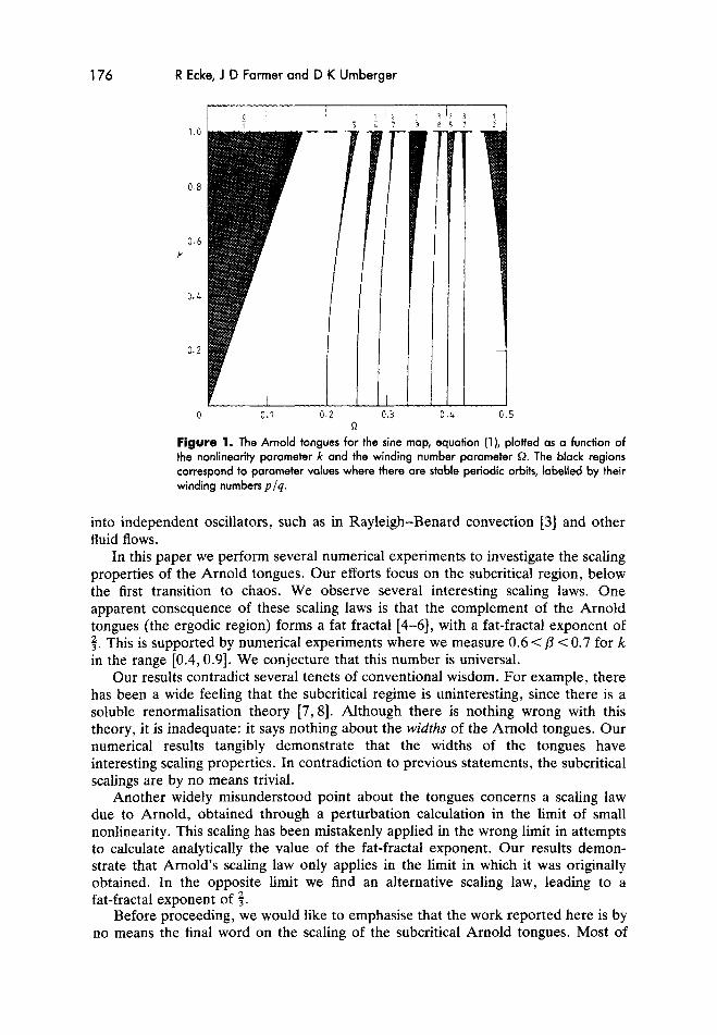
The phenomenon of mode locking is ubiquitous in physical systems. When two oscillators are coupled together they often entrain each other, so that their combined motion becomes periodic. In other cases, though, this does not happen, and their combined motion has two independent frequencies. Typically these locked and unlocked regions are interwoven in a complicated fashion in parameter space, as shown in figure 1. The black regions, called the Arnold tongues, represent the mode-locked parameter values [I]?. This basic scenario is quite common, and often manifests itself even when there is no obvious way to decompose the system

Even more general results have been proved in [Z].

0951 -771 5/89/01 O m + xxJi02.50 0 1989 IOP Publishing Ltd and LMS Publishing Ltd 175

176 R Ecke, J D Farmer and D K Umberger

1.0

0.8

0 . 6 k

0.4

0.2

0 0.1 0.2 0.3 0 . 4 R

0 .5

Figure 1. The Arnold tongues for the sine map, equation ( l ) , plotted as a function of the nonlinearity parameter k and the winding number parameter Q. The black regions correspond to parameter values where there are stable periodic orbits, labelled by their winding numbers p / q .

into independent oscillators, such as in Rayleigh-Benard convection 131 and other fluid flows.

In this paper we perform several numerical experiments to investigate the scaling properties of the Arnold tongues. Our efforts focus on the subcritical region, below the first transition to chaos. We observe several interesting scaling laws. One apparent consequence of these scaling laws is that the complement of the Arnold tongues (the ergodic region) forms a fat fractal [4-61, with a fat-fractal exponent of $. This is supported by numerical experiments where we measure 0.6 < /3 < 0.7 for k in the range [0.4,0.9]. We conjecture that this number is universal.

Our results contradict several tenets of conventional wisdom. For example, there has been a wide feeling that the subcritical regime is uninteresting, since there is a soluble renormalisation theory [7,8]. Although there is nothing wrong with this theory, it is inadequate: it says nothing about the widths of the Arnold tongues. Our numerical results tangibly demonstrate that the widths of the tongues have interesting scaling properties. In contradiction to previous statements, the subcritical scalings are by no means trivial.

Another widely misunderstood point about the tongues concerns a scaling law due to Arnold, obtained through a perturbation calculation in the limit of small nonlinearity. This scaling has been mistakenly applied in the wrong limit in attempts to calculate analytically the value of the fat-fractal exponent. Our results demon- strate that Arnold’s scaling law only applies in the limit in which it was originally obtained. In the opposite limit we find an alternative scaling law, leading to a fat-fractal exponent of $.

Before proceeding, we would like to emphasise that the work reported here is by no means the final word on the scaling of the subcritical Arnold tongues. Most of

Scaling of the Arnold tongues 177

our results are empirical, based on numerical experiments performed on only one circle map. Some of the properties that we observe suggest universal behaviour, but obviously more work on other maps is needed. But what is particularly needed is a theory. We hope that, although incomplete, the results that we present here are suggestive enough to stimulate further work in this direction.

Before proceeding further we present a brief review.

2. A few essential facts about circle maps

In geometric terms, a dissipative oscillator whose asymptotic motion is periodic is nothing more than a dynamical system with a limit-cycle attractor. Thus, its asymptotic motion is represented by a closed curve in its phase space, topologically equivalent to a circle. When two oscillators are coupled together, the natural space in which to consider their combined asymptotic motion is the direct product of two circles, i.e. a 2-torus. When the oscillators mode lock, the attractor of the combined system is a limit cycle embedded on the torus, and when they unlock the trajectory is ergodic, densely covering the torus.

Taking a PoincarC section reduces the torus to a circle. The flow on the torus in this surface of section becomes an iterated mapping of the circle with a single iteration of the resulting circle map corresponding to a complete revolution about one axis of the torus. This description breaks down for more complicated attractors, such as chaotic attractors. As long as the attractor is a limit cycle or torus, however, the dynamics can be reduced to a circle map?.

In general it is difficult to obtain the explicit form of a circle map directly from equations of motion. But qualitative studies can be made by explicitly constructing a circle map, with the knowledge that there is an infinite family of continuous coupled oscillators corresponding to this map. An example of such a map which has received a great deal of attention is the sine map, given by

x , + ~ = f ( x t ) = xt - (k/2n) sin(2nxJ + 52

where t is an integer labelling the number of iterations, and k and 52 are parameters. Equation (1) satisfiesf@ + 1) = f ( x ) + 1, as it must to be a map of the circle.

A quantity of particular interest is the winding number

p = lim (x , - x,) / t . (2) t-+m

When the nonlinearity parameter k = 0, the sine map reduces to a simple rotation of the circle with winding number 52. For irrational values of 52 there is a single ergodic orbit covering the circle, and at rational values there is a one-parameter family of periodic orbits parametrised by the initial condition xo. Thus, the periodic orbits have zero measure in 52, while the ergodic orbits take up the full measure. When k is increased above zero, the one-parameter family of periodic orbits is destroyed. Instead, as long as 0 < k S 1, for a given s2 the sine map has a unique attractor which is either a limit cycle of period q, or an ergodic orbit covering the circle. The limit cycles have rational winding numbers p / q , where p and q are two integers that

Of course, geometric properties, such as the time to cross successive Poincark sections, are not described by the circle map, but otherwise the dynamics on the circle map is topologically equivalent to that of the original flow.

178 R Ecke, J D Farmer and D K Umberger

are relatively prime. At any fixed k, 0 < k 6 1, each rational ratio p / q occupies an interval in 52. We call these periodic intervals. Viewed in the k, 52 plane, the set of all periodic intervals forms an infinite number of long thin ‘tongues’, each of which is widest at k = 1, contracting down to a point at k =0, as shown in figure 1. Numerical experiments [9-111 indicate that the combined measure of the periodic intervals is one at k = 1. Thus, in varying k from 0 to 1 the combined measure of the periodic intervals also changes from 0 to 1. At any fixed k in the range [0,1] the periodic intervals are dense in &, i.e. given any value of & there is always a periodic window arbitrarily nearby.

The Arnold tongues are naturally labelled by their winding number p / q . In order to understand the properties of the Arnold tongues, it is useful to organise their winding numbers using a construction called the Farey tree. Given two rational numbers of the form p l / q l and p 2 / q 2 , their Farey daughter is given by their Farey sum ( p l + p 2 ) / ( q l + q2). Starting with the values 0/1 and 1/1, by taking Farey sums it is possible to construct all the rational numbers in [0, 11. Through this process these rational numbers are naturally arranged in a binary tree, with 1/2 at the top of the tree, 1/3 and 2/3 branching out from it, and so on. Every number has two Farey parents; one of these, which we will refer to as the immediate parent, is one level higher in the tree, while the other parent is two or more levels up [12].

Sandwiched in between the Arnold tongues are the parameter values with irrational winding numbers, where the attractor is ergodic and covers the circle. We will call these parameter values the ergodic set. The fact that the periodic intervals are dense immediately implies that their complement is a Cantor set. (Thus for a two-parameter circle map such as (l), the ergodic set is topologically the Cartesian product of a Cantor set and a line interval.) For k = 1, numerical experiments [9-111 indicate that the Cantor set is thin, i.e. that it has Lebesgue measure zero. The fractal dimension is approximately equal to 0.87 and is believed to be universal [9,10, 131. For k < 1, however, the Cantor set is fat, i.e. it has positive measure. This implies that the fractal dimension is 1. The dimension is thus indistinguishable from that of a simple Euclidean set such as a line interval.

3. A brief review of fat fractals

As discussed in [4-6,14-191, the inadequacy of the dimension is a problem for fat Cantor sets and their more general counterparts, fat fractals, i.e. fractals with positive Lebesgue measure. The fact that a set has positive Lebesgue measure automatically implies that its fractal dimension is an integer. As a result, for fat sets the fractal dimension gives no information about fractal properties. An alternative is to examine the scaling of the coarse-grained measure p ( ~ ) , where E is the resolution, i.e. the scale of the coarse graining?. For thin fractals, p ( 0 ) = 0, and the leading-order scaling of the coarse-grained measure is a simple power law in E , i.e. p ( ~ ) where df is the fractal dimension, D is the dimension of the space in which the fractal is embedded and A is some positive constant. For fat fractals, it seems to be the case$ that the leading-order scaling in the limit as E+ 0 also goes as

t The possibility of power-law scaling for fat fractals was originally suggested by Mandelbrot [4]. This idea was made more explicit and extended in [5, 6, 14-19]. $ Although it is possible to construct examples for which this power-law scaling is violated, these appear to be unphysical (see [19]).

Scaling of the Amold tongues 179

a power law, except that it has a finite asymptote p(O) , i.e.

p ( ~ ) = p ( 0 ) + A & @ (3) where A and p are constants. A is unimportant, depending on the units of E and p . The exponent p, on the other hand, is independent of the choice of units and is an important quantity, providing a characterisation of fractal properties. For fat fractals @ is generally unrelated to the fractal dimension.

The exact definition of p depends upon the method of coarse graining, and several different methods have been proposed [5,6,14,15,17]. However, under certain quite general conditions, relationships between the resulting exponents exist, and the decision of which one to use can be based on convenience [18,19].

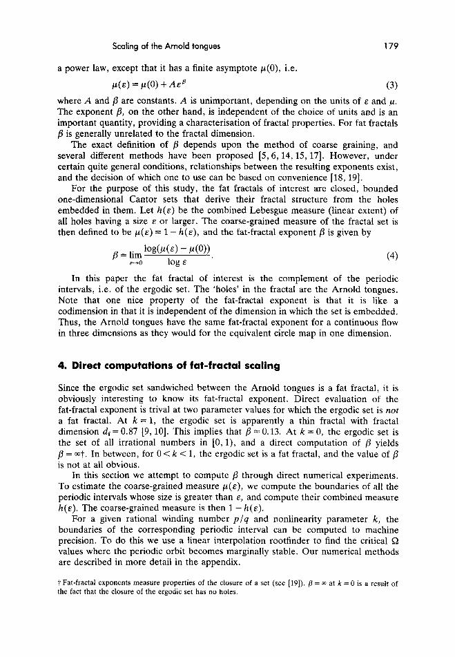
For the purpose of this study, the fat fractals of interest are closed, bounded one-dimensional Cantor sets that derive their fractal structure from the holes embedded in them. Let h ( ~ ) be the combined Lebesgue measure (linear extent) of all holes having a size E or larger. The coarse-grained measure of the fractal set is then defined to be p ( ~ ) = 1 - /I(&), and the fat-fractal exponent p is given by

E - 0 log E (4)

In this paper the fat fractal of interest is the complement of the periodic intervals, i.e. of the ergodic set. The ‘holes’ in the fractal are the Arnold tongues. Note that one nice property of the fat-fractal exponent is that it is like a codimension in that it is independent of the dimension in which the set is embedded. Thus, the Arnold tongues have the same fat-fractal exponent for a continuous flow in three dimensions as they would for the equivalent circle map in one dimension.

4. Direct computations of fat-fractal scaling

Since the ergodic set sandwiched between the Arnold tongues is a fat fractal, it is obviously interesting to know its fat-fractal exponent. Direct evaluation of the fat-fractal exponent is trival at two parameter values for which the ergodic set is not a fat fractal. At k = 1, the ergodic set is apparently a thin fractal with fractal dimension df = 0.87 19, 101. This implies that 0 = 0.13. At k = 0, the ergodic set is the set of all irrational numbers in [0, l ) , and a direct computation of 0 yields p = m t . In between, for 0 < k < 1, the ergodic set is a fat fractal, and the value of p is not at all obvious.

In this section we attempt to compute 0 through direct numerical experiments. To estimate the coarse-grained measure ,U(&), we compute the boundaries of all the periodic intervals whose size is greater than E , and compute their combined measure h ( ~ ) . The coarse-grained measure is then 1 - h ( ~ ) .

For a given rational winding number p / q and nonlinearity parameter k, the boundaries of the corresponding periodic interval can be computed to machine precision. To do this we use a linear interpolation rootfinder to find the critical Q values where the periodic orbit becomes marginally stable. Our numerical methods are described in more detail in the appendix.

t Fat-fractal exponents measure properties of the closure of a set (see [19]). @ = m at k = 0 is a result of the fact that the closure of the ergodic set has no holes.

180 R Ecke, J D Farmer and D K Umberger

To compute p( E ) it is important that we find all the periodic intervals whose sizes are greater than E. In order to be sure that we find all of them we organise the rational winding numbers using the Farey tree, as described in 42 [12]. Based on many numerical experiments, we find that any given periodic interval is always smaller than the periodic interval corresponding to its immediate parent in the Farey tree. Assuming this is true, it gives a systematic procedure for computing all of the stability intervals larger than a given size. Starting with p = 0 and p = 3 we systematically explore every possible path? down the tree, stopping whenever we encounter a stability interval whose width is less than E. This results in a tree with a very jagged bottom, as shown in figure 2.

R

0 . 5

0.4

0 . 3

0 .2

0 . 1

E ' , . : I

.......... """""""""

k : 1.0

. . . . .

. , . . .

. . . . . .

I l l . . . . . . . . . . . . .

3 20 40 60 L e v e l

Figure 2. An illustration of the Farey tree construction applied to the sine map. The vertical axis corresponds to the winding number parameter a, and the horizontal axis corresponds to the depth in the Farey tree. We plot only values corresponding to periodic intervals whose size is greater than E = As can be seen, this results in a tree with a very jagged bottom, illustrating the complicated dependence of ASL on the position in the Farey tree. The difference in the scalings of the critical ( k = 1.0) and subcritical ( k = 0.8) cases is also apparent. For the critical case there are many more large intervals. The subcritical Farey tree is dominated by the intervals with winding number I /q .

f Due to the symmetry of the mapping of (l), the periodic intervals corresponding to p in [0, i] are identical in size and distribution to those corresponding to p in [i, 11.

Scaling of the Arnold tongues 181

I I

10-8 10-6 E 10-2

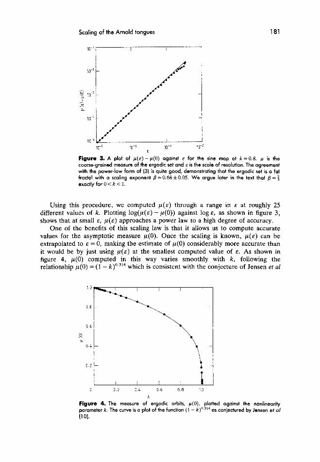
Figure 3. A plot of p ( ~ ) - p(0) against E for the sine map at k = 0.8. p is the coarse-grained measure of the ergodic set and E is the scale of resolution. The agreement with the power-law form of (3) is quite good, demonstrating that the ergodic set is a fat fractal with a scaling exponent /3 = 0.68 f 0.05. We argue later in the text that fi = I exactly for 0 < k < 1.

Using this procedure, we computed p ( ~ ) through a range in E at roughly 25 different values of k. Plotting log(p(E) - p ( 0 ) ) against log E , as shown in figure 3, shows that at small E , p ( ~ ) approaches a power law to a high degree of accuracy.

One of the benefits of this scaling law is that it allows us to compute accurate values for the asymptotic measure p(0 ) . Once the scaling is known, p ( ~ ) can be extrapolated to E = 0, making the estimate of p ( 0 ) considerably more accurate than it would be by just using p ( ~ ) at the smallest computed value of E. As shown in figure 4, p ( 0 ) computed in this way varies smoothly with k , following the relationship p ( 0 ) = (1 - k)".314 which is consistent with the conjecture of Jensen et a1

I I I I 0 0.2 0.4 0.6 0.8 1.0

k

Figure 4. The measure of ergodic orbits, p(O), plotted against the nonlinearity parometer k . The cuwe is a plot of the function (1 - k)".3'4 as conjectured by Jensen et a/ 11 01.

182 R Ecke, J D Farmer and D K Umberger

[lo], based on data for values of k in the range 10.9, 1.01. However, our results indicate that their conjecture is valid through the entire subcritical region of k.

The consistency of our result for p(0) as a function of k with that of Jensen et a1 is somewhat surprising. The data they use to support their result also suggests other scaling laws that, when cast into the language of fat fractals, lead to a prediction that p = 1. This is incompatible with our numerical observation that 0.6</3 <0.7 for 0.4 < k < 0.9.

Though p(0) is quite easy to obtain, it is more difficult to get an accurate value for the scaling exponent p. There are several difficulties. One of them has to do with numerical limitations on gathering data near k = 0 . In this region the combined measure of the periodic intervals is quite small, and there are very few periodic intervals larger than machine precision. As a result we have almost no data on the fat-fractal scaling behaviour when k < 0.4.

Yet another problem in computing /3 occurs due to slow convergence near k = 1. The underlying reason for this comes from a crossover effect associated with the transition from a fat fractal to a thin fractal at k = 1. This crossover effect is easily seen by numerically differentiating the data for the plot of log p ( ~ ) against log E and plotting the result as a function of log E, as shown in figure 5 . For the data at k = 0.8 the computed derivative converges fairly quickly to a value near p = 0.68. For k = 0.95, in contrast, the asymptote is never reached; at the smallest values of E the computed derivative is still changing, making it difficult to estimate the asymptotic value of p. This problem becomes more pronounced as we approach k = 1.

As a result of these problems we can only compute /3 accurately in the range 0.4 < k < 0.9. Taking into account the sources of error discussed above, in this range we estimate p = 0.68 f 0.05. This leaves several important questions unanswered, the most basic being: is the value of /3 constant through a range of k values, or does it vary with k? This question is particularly interesting in view of the ‘phase

0.70 I I I I

0.65 t = c 0.55

0

0

0

. . * *

l

0

0

0

1 . *

0.50 L I I I n , I

IO-’ IO-^ 10- 1 0 - b 10-3 10-2 E

Figure 5. An illustration of the convergence of the computed value of the fat-fractal scaling exponent /3 with the scale of resolution E. The numerical data of figure 3 are numerically differentiated. The resulting slopes are plotted against the corresponding values of log&, to give an idea of the rate of convergence. We show two cases. At k = 0.80 (0) the convergence is within experimental error at the smallest values of E. At k = 0.95 (0), however, due to crossover phenomena there is no convergence, even at the smallest value of E that we were able to compute.

Scaling of the Amold tongues 183

I

0.25

e e e

-

8 I I I I

0 0.25 0.50 0.75 1.00 1.25 k

Figure 6. Computed values of the fat-fractal exponent /3 plotted against the nonlin- earity parameter k . In the range where we have reliable data the computed value is close to 3 . Near k = 1, however, cross over phenomena such as that shown in figure 5 prevent us from being able to get accurate estimates. Thus, we feel that the apparent smooth transition to criticality is due to crossover effects, and the true value of /3 is $ (broken line) throughout 0 < k < 1.

transition’ from a fat fractal to a thin fractal at k = 1. At k = 1 we know that p is the complement of the fractal dimension, which according to the computations of Jensen et a1 [9, 101 has a value of p = 0.13. This is substantially different from the value of 0.68 observed at k = 0.9. What happens in between? Is there a discontinuous jump, or does the value change continuously?

A brute force computation of the exponent at different values of k, as shown in figure 6, suggests a smooth transition. However, we believe that this is entirely a crossover effect, and that the exponent takes on the constant value /3 = i.

5. Numerical evidence supporting scaling laws for AQ(q,fi, k)

Arnold [l] has studied the behaviour of the stable periodic intervals for (1). In particular, he proved that

A Q c Ckq (5 ) where C is a constant. For small k and q, this upper bound is actually a very good estimate?, as shown in figure 7, where we plot the logarithm of A Q against the logarithm of k. For q = 1 the kq law is exact throughout the entire subcritical region of (1). For larger values of q, however, deviations begin to appear at large k, as can be seen by examining the upper right-hand part of the figure; the upper bound ceases to be a good estimate. As q increases, deviation becomes more severe, so that for very large values of q it is numerically impossible to get close enough to k = 0 to observe kq scaling at all. The breakdown of the kq law for sufficiently large values of k and q is illustrated in more detail in figure 8, where we give similar plots for q = 10, 15 and 20.

t See [lo] also.

184 R Ecke, J D Farmer and D K Umberger

1

1 0 - ~ IO+ 10-2 I@-’ 1 k

Figure 7. According to Amold [l 1, in the limit as k- , 0 at fixed q, A Q = k9, for q = 1 , 2 or 3. In this figure we see that this works quite well, even for larger values of q. AQ is the width of a given periodic interval, k is the nonlinearity parameter, and q is the period. The ratio shown near each curve is the winding number.

I I

Another interesting limit, relevant to fat-fractal properties, is when q 4 m while k is held fixed. To investigate this limit, we plot the logarithm of AQ against the logarithm of q, with p = 1, for several different values of k, as shown in figure 9. This plot reveals a very different behaviour: the curves approach a straight line, indicating that AQ scales as a power law in q. Measurements of the asymptotic slope of these curves yield powers that in every case are extremely close to -3 (for example, at k = 0.8 we measured the slope as -2.9998 f 0.0004). This scaling is not restricted to winding numbers with p = 1, as can be seen in figure 10, where we plot log As2 against log q for several different values of p at k = 0.8. This leads us to hypothesise that, in the limit as q 4 CQ at fixed k,

A Q = Cq-3

where C is some constant of proportionality. Note that Kaneko has observed a

lo- ’ 1

Figure 8. Arnold‘s scaling law breaks down for large k or q, as seen in this figure, which is like figure 7 except that q is larger.

Scaling of the Amold tongues 185

I

10-5 1 I

1 10 lo2 i o 3 1 4

Figure 9. The widths of periodic intervals plotted agoinst the period q , for intervals with winding number l / q , at several different values of the nonlinearity parameter k . For large q the data approach a straight line of slope -3. This convergence is slower at smaller k, corresponding to a crossover to Amold’s kq scaling. A, k = 1.0; 0, k = 0.8; B, k = 0.65; 0, k = 0 . 5 ; A, k = 0 . 4 ; 8, k = 0 . 3 ; 0 , k = 0 . 2 .

similar relationship?. The dependence of C on p and k is indicated in figures 9 and 10, respectively, where we see that different values of these quantities result in different intercepts.

This power-law scaling is particularly interesting when compared with the result [lo, 121 obtained for critical maps ( k = 1). They demonstrate that

lim q3AQ = constant q-m

which is the scaling that we observe, except that we are seeing this same scaling in the subcritical regime. This is somewhat surprising, since the argument that

1 IO‘ 102 103 lo4 105 Q

Figure 10. For a given nonlinearity parameter k = 0.8, AB is plotted against the period q for several different values of p . For large q the asymptotic scaling goes as q-3.

t Kaneko has previously observed a similar relationship, of the form Ak = Cq-3. If AB is proportional to Ak, then these two results are equivalent. See [20].

186 R Ecke, J D Farmer and D K Umberger

Cvitanovic et a1 [12] use to derive this result explicitly assumes criticality. In particular, they assume that the periodic intervals and their neighbourhoods are self-similar, i.e. that the separation between the centres of two periodic intervals with winding numbers l / q and l / (q + 1) scales like AQ(1, q). For critical maps this is true, but for subcritical maps there is nothing in existing renormalisation theories to suggest that this should be so. Thus there is no a priori reason to suspect that the 4 - 3 scaling should hold in general, and this numerical result is surprising.

It is immediately apparent that the domain of validity of the q-3 law is quite different from that of the kq law. They cannot be exactly valid at the same time, since at fixed k, (6) implies exponential scaling in q. The key point is that Arnold’s calculation is an upper bound, and is a good estimate only in the limit as k - 0 at fixed q. The 4 - 3 law, in contrast, is valid in the opposite domain, i.e. as q+w at fixed k. The difference in the domains of validity can be seen by comparing figure 9 with figures 7 and 8. In the latter two figures we see that the kq law is not satisfied when k and q are large, and in figures 9 and 10 we see that the q-3 law is not satisfied when k and q are small. Thus, these scaling relations are valid in complementary regions of the parameter space, with a crossover in between.

To summarise, our numerical experiments suggest that for fixed p and a fixed value of k in (0, 11, AQ scales as q-3 in the limit as q + 03, but in the limit as k + 0 for fixed q AQ scales exponentially in q.

5.1. Scaling of AQ as a function of p and q at fixed k

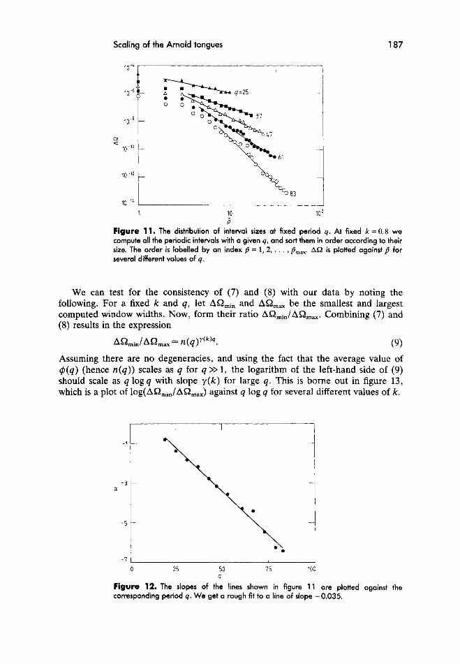
In the previous subsection, we found that AS2 scaled as q-3 for fixed k. Unfortunately, numerical study reveals that at fixed q there is a wide discrepancy in the values of AQ produced by different values of p . The behaviour is not monotonic in p , i.e. the values of AQ fluctuate wildly as p increases, making it clear that the dependence of AQ on p is quite complicated. To avoid this problem, we seek a statistical law. By reordering the AQ values according to their size, they can be assigned labels p which indicate their order in size. For convenience, we let p’ = 1 correspond to the largest window, p = 2 correspond to the second largest window, etc, and = n(q) correspond to the smallest window. When there is no degeneracy in window sizes, n(q) =$#(q ) where #(q ) is the Euler-Totient function whose values are the number of integers not exceeding q that are relatively prime with respect to q. The results of this reordering process are shown in figure 11, where we show the size distributions at k = 0.8, for several different values of q. We have experimented with various ways of plotting our results, and found that, for each fixed q, the data is reasonably well represented by a power law of the form

where C is a constant. As seen in figure 11, equation (7) gives a fairly good fit for large p , but there are significant deviations when p is small, particularly for large q.

The variation of the exponent with q is shown in figure 12, where we plot a(q) against q. We see that

where y ( k ) G 0.

Scaling of the Arnold tongues 187

' O - i - 10-6

2 c 10-l0

I 10 - 1 2

-1

10-lL 1 1 I 1 10 IO2

P Figure 11. The distribution of interval sizes at fixed period q . At fixed k = 0.8 we compute all the periodic intervals with a given q, and sort them in order according to their size. The order is labelled by an index a = 1, 2, . . . , a,,,. A Q is plotted against p for several different values of q .

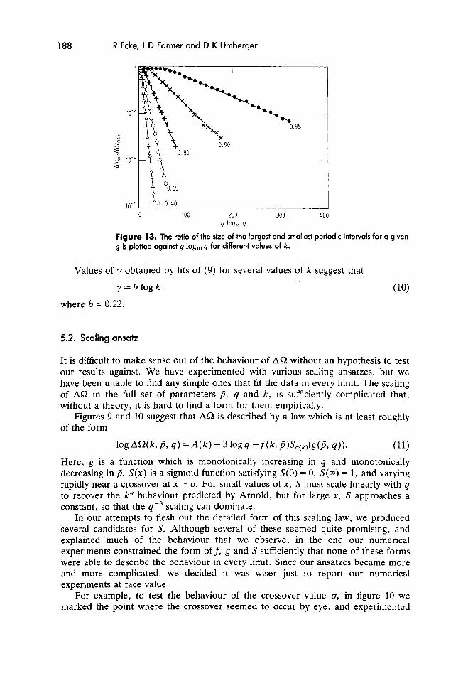
We can test for the consistency of (7) and (8) with our data by noting the following. For a fixed k and q, let ABmin and AB,,, be the smallest and largest computed window widths. Now, form their ratio ASZ,in/AB,,,. Combining (7) and (8) results in the expression

AB,in/AB,,, = r ~ ( q ) " ( ~ ) ~ . (9) Assuming there are no degeneracies, and using the fact that the average value of $(q) (hence n(q)) scales as q for q >> 1, the logarithm of the left-hand side of (9) should scale as q log q with slope y ( k ) for large q. This is borne out in figure 13, which is a plot of log(ABmin/ABm,,) against q log q for several different values of k.

a

1

-1 -

- 3 -

.- - 5 -

0 25 50 75 100

Figure 12. The slopes of the lines shown in figure 1 1 are plotted against the corresponding period 9 . We get a rough fit to a line of slope -0.035.

-1

4

188 R Ecke, J D Farmer and D K Umberger

1

10-2

e 4

a

c

l 0 - L

I I

0 100 200 300 400 4 log,, 4

Figure 13. The ratio of the size of the largest and smallest periodic intervals for a given q is plotted against q log,, q for different values of k .

Values of y obtained by fits of (9) for several values of k suggest that

y = b l o g k (10)

where b "- 0.22.

5.2. Scaling ansatz

It is difficult to make sense out of the behaviour of AS2 without an hypothesis to test our results against. We have experimented with various scaling ansatzes, but we have been unable to find any simple ones that fit the data in every limit. The scaling of AS2 in the full set of parameters p , q and k , is sufficiently complicated that, without a theory, it is hard to find a form for them empirically.

Figures 9 and 10 suggest that AS2 is described by a law which is at least roughly of the form

Here, g is a function which is monotonically increasing in q and monotonically decreasing in 15. S(x) is a sigmoid function satisfying S(0) = 0, S(m) = 1, and varying rapidly near a crossover at x = U. For small values of x, S must scale linearly with q to recover the k4 behaviour predicted by Arnold, but for large x, S approaches a constant, so that the q-3 scaling can dominate.

In our attempts to flesh out the detailed form of this scaling law, we produced several candidates for S. Although several of these seemed quite promising, and explained much of the behaviour that we observe, in the end our numerical experiments constrained the form off, g and S sufficiently that none of these forms were able to describe the behaviour in every limit. Since our ansatzes became more and more complicated, we decided it was wiser just to report our numerical experiments at face value.

For example, to test the behaviour of the crossover value 0, in figure 10 we marked the point where the crossover seemed to occur by eye, and experimented

Scaling of the Amold tongues 189

IO+

with different ways of plotting the data. When we plot log ASZ against q / p the crossovers all occur at roughly the same place. This suggests that g@, q ) = 4/15, and U is a function of k alone. To get an idea of the k dependence we measured the asymptotic y intercepts f(k) of the lines approached by the curves in figure 9. We get a good fit when we plot f(k) against l lk, giving the approximate relationship

f(k) = -2.69(l/k - 1.09). (12) This is of course only approximate; since it vanishes close to k = 1, it may well be that the last term is exactly 1 rather than 1.09. Also, this may only be the lowest-order term in a Taylor expansion of something else. Since we cannot probe to small values of k it is difficult to tell.

Another test of the scaling comes from plotting AS1 against log k for different values of (see figure 14). The striking result is that we still see k4 scaling, independent of 15. Changing p only causes a shift in the ASZ intercept. This places a strong constraint on the form of So.

Finally, it is interesting to study the behaviour of ASZ at criticality. Figure 13 and equation (10) make it clear that there is a qualitative change in the behaviour there, as y (the slope) apparently goes to zero. In fact, by replotting the data at k = 1, we see that ASZmin/ASZm, roughly follows a power law, with an exponent that is approximately 0.72, as illustrated in figure 15.

Another important qualitative change has to do with the meaning of the variable 15. Well below criticality we find that AQ,,, always corresponds to p = 1, so that 15 = 1 implies p = 1. This is illustrated in figures 16(a) and 16(b), where we plot log ASZ against log q for many different values of p, at k = 0.8 and 0.9, respectively. In both cases, the top ‘line’ of dots corresponds to p = 1. As we increase k to 0.95 this changes; the lines of dots corresponding to p = 1 is now in the middle, and the top edge now corresponds to another value of p, as shown in figure 16(c). This effect continues to grow, until in figure 16(d), for k = 0.99 we see that the line p = 1 now corresponds to the smallest ASZ within the range of log q shown!

d I I

10.‘

10 - 9

c a

10-12

190 R Ecke, J D Farmer and D K Umberger

10.. I I 1 IO0 10' O IO' IO' O 10'

9 Figure 15. The ratio of the sizes of the largest and smallest periodic intervals for a given q i s plotted against q for k = 1. Compare with figure 13.

c a

I I (c l

I O ' & I- -1 c I

' I 1 I

(el - - 2

I " - t 1

1 o - 6 lo' lo2

Q

1

10' 102 q

Figure 16. We plot AQ against q for as many values of q and p as we can conveniently compute, for (a) k = 0 . 8 , (b) k = 0 . 9 , ( c ) k=0.95 , (d) k = 0.99 and (e ) k = 1.0. As we move towards critica- lity, the p = 1 line moves from the top to the bottom, and the exponential falloff of the bottom edge becomes slower, until finally at criticality both edges are described by power laws. At criticality, the slope of the tap edge is apparently Shenker's 6 = -2.16, while the slope of the bottom edge is -3.

Scaling of the Amold tongues 191

Nonetheless, note how the top edge of the ‘envelope’ described by all of the points continues to be parallel to the line defined by p = 1. This implies that p = constant still asymptotically follows the qW3 law very close to criticality, at least for low values of p .

This dramatically shifts at k = 1, as seen in figure 16(e). Now the lower boundary of the envelope is straight, indicating that now both follow power laws. The lower boundary is defined by p = 1, which has slope -3. In the middle we see other lines defined by different values of p = constant, which also have slope -3. However, the top edge, which by definition corresponds to p = 1, has a different slope, which is approximately Shenker’s 6 = -2.16. The explanation is that the value of p corresponding to p = 1 is constantly shifting, as we follow the golden mean scaling through the Farey tree, so that even though any fixed p follows slope -3, the top edge is not as steep. The average scaling for any given q lies somewhere in the middle, corresponding to the mean scaling exponent -2.29 measured by Jensen et a1 [lo]. Presumably this can also be related to the average scaling exponents observed in renormalisation experiments in which the scaling is not restricted to the golden mean [21,22].

To conclude: we have discovered a variety of different scaling relationships, corresponding to various limits and cuts through the parameter space of AQ@, q, k ) . The most important scaling relationship is that, in the limit as q + CQ at fixed p and k, AS2(q) = Cq-3.

At this point, we do not have a theory, and it is difficult to go much further without one. Nonetheless, the scalings and the ansatz that we have presented provide a variety of constraints that any theory must satisfy. We have certainly demonstrated that the subcritical scaling behaviour for the widths of the windows is not ‘trivial’. Also, we have enough information about the scaling to compute the value of the fat-fractal exponent p.

6. Estimate of fat-fractal scaling exponent from properties of AQW, 4)

Although our numerical work in the previous section did not determine a complete expression for AQV, q ) , we know enough about its asymptotic behaviour as q and p go to infinity at fixed k to estimate the fat-fractal exponent /3 analytically. The essential scaling relationship that dominates the fat-fractal scaling is the limiting behaviour as q --j m at fixed p and k. Based on our numerical studies, we are quite confident that in this limit AQ decreases according to q-3 for subcritical values of k. The other essential fact that emerges from our numerical experiments is that, for fixed k and q, AS2 decreases in p’ faster than a power law for p << q and as a power law with a large exponent (proportional to q ) for larger values of p . As we shall see, this very fast drop-off of AS2 with p together with the qW3 scaling determines the value of p.

To begin the calculation, we note that dp(&)=p(&)-p(O) of (3) is just the measure of all periodic intervals which are smaller than E. Fixing the value of E << 1, we have

W E ) = c A Q ( q , P ) AQ<E

where the sum is over all values of q and f i for which the inequality holds.

192 R Ecke, J D Farmer and D K Umberger

To understand the behaviour of this sum, we make the ad hoc assumption that

(14) AQ = Aq-3p’- a

where A and a are positive constants. Although this is not the correct form, what we will demonstrate is that, providing A Q falls to zero in p’ sufficiently rapidly, the asymptotic scaling is dominated by the q-3 behaviour, so that the fat-fractal exponent p takes on the same value independent of any detailed assumptions about the p’ dependence.

The domain of the summation is sketched in figure 17. For convenience we have broken it into two regions. In region I the lower boundary is given by AQ = E ,

which in this case gives

qc = ( ~ p ’ a/A)-1/3.

The lower boundary of region I1 is determined by the fact that < q. This condition is a bit complicated, since some values of p may yield reduced fractions, so that, unless q is prime, Pmax < q - 1. This can be taken into account on average using the fact that, in the limit of large q, the fraction of integers p”,, that are prime relative to q is pmax = 3/;n2q. For the purposes of our estimate we will simply use pmax = q since the factor 3/n2 does not affect the calculation-any fixed value yields the same result.

The vertical line @ = p * divides the two domains. p * is determined by qc(q p * ) = p * , which gives

(16) p * = ( E / ~ ) - 1 / ( 3 + 4 .

Summing over each region, we have

These sums can be estimated by converting them into integrals. Doing this in the most straightforward way results in a lower bound on dp(&), since AQ is a

Figure 17. The domain of the summation given in (1 9). q is the period, p is the size-ordered numerator of the winding number, qc is the critical curve where A Q = E, and p * is the p value such that qc = p.

Scaling of the Arnold tongues 193

monotonically decreasing function of q and p . Later we will compute an upper bound.

Converting these sums to integrals gives

6 p ( t ) = [ * r A q - ] p ' - " d p d q q c + I:: 5 4 q - 3 P - Y dq. (18)

Using (15) for qc and (16) for p * , these integrals are straightforward. Providing a Z 3 and a# -1, the result is

(19) ( ~ ~ ( ~ 1 = cE2/3 + & ( m + l ) / ( n + 3 )

where C and are constants. As long as a > 3 , the first term asymptotically dominates in the limit as E+O.

This scaling comes from a lower bound on G ~ ( E ) . Since AS2 is monotonic decreasing, an upper bound can be constructed by integrating AS2@ - 1, q - 1) over the same limits used in (18). This creates a problem at p = 1, since AS2(O, q ) = 00.

This problem can be solved by explicitly separating the p = 1 term, so that

@ ( E ) s [ A(q - 1)-3 dq + -/ -/ A(q - l)-3@ - l)-m dp dq P' -

q e 2 q c

r m rm + A(q - l)-3(p' - l)-a dp dq.

The first term comes from 15 = 1. Doing this integral shows that, as long as a > 3, this term continues to dominate, so that the leading-order scaling goes as E " ~ . Since we have demonstrated that G,u(E) has both upper and lower bounds that scale as E " ~ , it is clear that & ( E ) must scale that way as well.

Furthermore, it is clear that, providing AS2 falls off sufficiently fast as p + M at fixed q, the dominant scaling is &'I3. The first term in (20) is independent of p , and yields this scaling; as long as the other terms vanish fast enough, this term will dominate. The critical scaling occurs for a power-law dependence of the form of (14) with a = 3 . From our numerical studies it is clear that this is satisfied in the subcritical regime, since AS2 falls off as p +.m faster than p-3. It is also clear that, as long as the q-3 scaling holds, 3 is an upper bound for 0, regardless of the nature of the p scaling, since in the limit as E + 0, the lowest scaling exponent dominates. The p = 1 term generates a scaling exponent of 3, which guarantees that /3 s 3.

At criticality, as we have demonstrated in figure 16(e), p = 1 no longer corresponds to p = 1, and the q-3 scaling law is no longer the dominant scaling. Instead, the dominant scaling is q', where the exponent is Shenker's 6 = -2.16. However, since both boundaries of the envelope in figure 16(e) are described by power laws, there is no single dominant scaling, and it becomes necessary to take an average of the different scalings. We have not done this, but the average scaling that Jensen et a1 [lo] report is in agreement with the value p = 0.13 that is a consequence of their calculations of the fractal dimension.

Thus, we conclude that /3 = $ throughout the subcritical regime. This result is a consequence of the q-3 scaling, combined with the rapid asymptotic falloff of the p scaling. Note that this result is in agreement with our direct numerical calculations; prior to this computation, at the parameter values where we felt confident enough to make estimates (0.4< k<0 .9 ) all gave values within a few percent of 0.67. p discontinuously jumps to /3 = 0.13 at criticality. The transition from fat-fractal

194 R Ecke, J D Farmer and D K Umberger

scaling to thin-fractal scaling is like a first-order phase transition, even though in a naive numerical study it looks like a second-order phase transition, due to crossover effects.

Note that our result contradicts a previous result by Grebogi et a1 [14], who conjectured that p = 1 for all k < 1. Their mistake was the assumption that A Q ( q ) -- k4. As we stated in the previous section, this is true only for the limit as k -+ 0 at fixed q, whereas they assumed that it was true as q at fixed k. As we have shown, the q-3 scaling term combined with the rapid falloff window size with p implies that p s 5, in contradiction with their result.

8. Discussion

The most striking result of 9.5 is the q-3 scaling of AQ. Although we have not studied other maps, and so we cannot make a convincing statement in this regard, because of the simplicity of this result we feel that it is likely to be universal. It would be nice if someone could extend this result, either by more experiments on other systems or, better yet, by a theory. If true, this universality would be particularly interesting, since it does not come from a particular behaviour near a critical point. Of course, it may be that this is a special property of the sine map.

An interesting feature of this scaling is the correspondence? to the critical scaling discovered by Cvitanovic et a1 [12]. This aspect of the subcritical scaling is the same as the critical scaling. This is somewhat contrary to conventional wisdom, which comes from renormalisation theories which treat the behaviour of the centres of the periodic intervals [7,8,11]. These theories demonstrate that all subcritical maps approach the same universal behaviour, which is different from that of critical maps. The universal properties of the subcritical maps are ‘trivial’, in that they reduce to those of the simple rotation, which can be understood from number theory.

The behaviour that we have studied here relates not to the centres of the periodic intervals, but rather to their widths, AQ. As we have demonstrated, the scaling of the widths does not appear to be trivial. Some aspects, such as the asymptotic q dependence, are the same as the critical behaviour. Other aspects, in particular the p dependence, are quite different from the critical behaviour; AS2 falls off much faster for the subcritical regime than it does in the critical regime. As a result, the fat-fractal properties are dominated by the q dependence in the subcritical regime. This is the origin of our conjecture that /3 = 3 throughout this regime.

Perhaps the main conclusion of our paper is that more attention should be devoted to theoretical treatment of the scaling properties of the subcritical Arnold tongues. In contrast to the critical surface, which is just a boundary between two regions of parameter space, the subcritical region occupies a finite portion of parameter space, and is easy to find experimentally. Many have assumed that the properties of the subcritical region are trivial, but our experiments suggest that there are many interesting scaling relationships.

?The part of their argument having to do with the scaling of the centroids applies equally well to the subcritical case. The part which does not is the assumption of self-similarity. It is surprising that the widths of the subcritical periodic intervals behave sufficiently like the centroids to make them scale the same way.

Scaling of the Amold tongues 195

Acknowledgments

We would like to thank V I Arnold and Predrag Cvitanovic for helpful comments. This work was partially supported by AFOSR grant ISSA-84-00017, and by the US Department of Energy Office of Basic Energy Science.

Appendix

We describe here the numerical methods used to generate the data discussed in the text. The first part deals with the calculation of the interval widths for a given p / q cycle of the sine circle map. The second part shows how the intervals can be calculated in an efficient manner taking into account the Farey-tree ordering of locking intervals. The mapping we consider here is the standard sine circle map but the techniques are general and can be applied to any mapping of a single variable which displays locking behaviour. The circle map is

x,,~ = x, + Q - (k/2n) sin(2nx,) (All

where Q is the bare winding number and k the nonlinearity parameter. We define f ( x , ) = x, + Q - ( k / 2 n ) sin(2nx,) so the map is now of the form x,+~ = f (x,). The condition for locking in a p / q cycle (k fixed) is f 9 ( Q $ x,) = p + x, where Q: is some value of Q in which the locking p /q is stable. xq denotes one of the q stable fixed points of the map, and f 4 ( x ) is the qth iterate of the function f ( x ) . We want to locate the marginally stable values of S2: which define the interval of stability of the p /q locking. The condition for this is that de,/&, = 0. This quantity can be written

dQ,/du, = (1 - a f w ~ , y ( a f v a ~ , ) .

a f w ~ , = af(x,)/ax af%m, = 1 + (af(~,_~)la~)(af9--’ia~,).

(A2)

In terms of derivatives of the mapping itself, af /ax, one can write

For each value of x in the interval 0 < x < 1 there exists a solution of equation (Al) for the parameter Q,. Therefore, we pick a value of x, calculate the value of Q,, and evaluate the function dQ,/&,. The zero of this function is found using a modified linear interpolation rootfinder which requires finding values of x which bracket the zero. We use this method rather than Newton’s method because it is certain to produce convergence and yet is only marginally slower.

As mentioned earlier in the text, we calculate intervals according to their distribution on the Farey tree rather than calculating all intervals with a given q and iterating the value of q. This is an advantage when computing the measure because one does not calculate many intervals smaller than the size of interest. The procedure used is to start with the intervals 0/1 and 1/1 and generate the successive Farey sums, defined as p / q = p ‘ / q ’ @p” /q ”= ( p ’ +p”)/(q’ + 4”). Thus the first interval down in the tree is 1/2, then 1/3 and 213, etc. We go down the 0/1 branch until we reach a smallest window size which we specify. Then we work our way back up that branch exploring all side branches as we go until we get back up to the interval 1/2. We only go to 1/2 since the particular map we use is symmetric about 1/2. This only works provided that the interval formed by the Farey sum is always

196 R Ecke, J D Farmer and D K Umberger

smaller than the intervals of the ‘parents’. We log all exceptions to this assumption in the program and have not found any exceptions for a variety of k values in the interval 0 < k < 1. The details of the computer program which generate the tree structure requires that the code be written in a recursive language such as c or PASCAL; FORTRAN does not work for this.

References

[ l ] Arnold V I 1961 Izv. Akad. Nauk Ser. Mat. 25 21; 1983 Usp. Mat. Nauk 38 189 (Engl. transl. 1983

[2] Galkin 0 1986 Dissertation Moscow University [3] Haucke H and Ecke R 1987 Physica 25D 307 [4] Mandelbrot B 1982 The Fractal Geometry of Nature (San Francisco: Freeman) [5] Farmer J D 1985 Phys. Rev. Lett. 55 351 [6] Umberger D K and Farmer J D 1985 Phys. Rev. Lett. 55 661 [7] Ostlund S, Rand D, Sethna J and Siggia E D 1983 Physica 8D 303 [8] Feigenbaum M J, Kadanoff L P and Shenker S J 1982 Physica 5D 370 [9] Jensen M H, Bak P and Bohr T 1983 Phys. Rev. Lett. 50 1637

Russ. Math. Surv. 38 215)

[IO] Jensen M H, Bak P and Bohr T 1984 Phys. Rev. A 30 1960 [ 111 Landford 0 1985 Physica 14D 403 [12] Cvitanovic P, Shraiman B and Soderberg B 1985 Phys. Scr. 32 263 [13] Cvitanovic P, Jensen M H, Kadanoff L P and Procaccia I 1985 Phys. Rev. Lett. 55 343 [14] Grebogi C, McDonald S W, Ott E and Yorke J A 1985 Phys. Lett. llOA 1 [15] Grebogi C, Ott E and Yorke J A 1986 Phys. Rev. Lett. 56 266

[16] Farmer J D 1986 Dimensions and Entropies in Chaotic Systems ed G Mayer-Kress (Berlin: Springer)

[17] Umberger D K, Mayer-Kress G and Jen E 1986 Dimemions and Entropies in Chaotic Systems ed G

[18] Eykholt R and Umberger D K 1986 Phys. Rev. Lett. 57 2333 [19] Eykholt R and Umberger D K 1988 Relating the various scaling exponents used to characterize fat

[20] Kaneko K 1983 Prog. Theor. Phys. 68 403 (211 Farmer J D and Satija I I 1985 Phys. Rev. A 31 3520 [22] Umberger D K, Farmer J D and Satija I I 1986 Phys. Lett. 114A 341

Farmer J D and Umberger D K 1986 Phys. Rev. Lett. 56 267

P 54

Mayer-Kress (Berlin: Springer) p 42

fractals in nonlinear dynamical systems Physica 30D 43-60