SCALING IN THE CLOUD FOR FLASH EVENTS WITH LEAD-LAG

FILTERS

A Thesis

Presented to the

Faculty of

California Polytechnic University, Pomona

In Partial Fulfillment

Of the Requirements for the Degree

Master of Science

In

Computer Science

By

Jonathan Mansur

2014

Acknowledgement

I would like to first thank my thesis adviser, Dr. Lan Yang, whose calm advice helped temper

the occasional deadline panic. Next a thank you for Dr. Daisy Sang and Dr. Gilbert Young

for agreeing to be committee members, in particular, their commitments of time and energy.

I would like to thank Dr. Mohammad Husain whose class in secure communications pushed

my ability to research, but more importantly how to communicate the fruits of that research.

I would also extend thanks to Dr. Ciera Jaspan, although she is no longer a member of the

Cal Poly Pomona Faculty, her classes in software engineering and verification & validation

greatly improved how I approach software development. What I learned from her about test

driven development alone would’ve saved me a lot of self inflicted misery if I had applied it

more consistently. Thanks to the faculty and staff of the Computer Science department of

Cal Poly Pomona for their exceptional teaching of the curious art of [hopefully ]controlling

computers. In addition, thanks to the faculty and staff of Cal Poly Pomona for providing

an excellent learning environment with a spacious campus that provides ample inspiration

for regular exercise when traveling between classes.

I would like to thank my parents, Rick and Carolyn, for being my first teachers, even

if I was unappreciative at the time. My mother for teaching me the art of learning and

my father for helping develop my early technical knowledge. Additionally, I would extend

thanks to my grandparents for their support over the years. From the large to the the small,

such as, nodding along as I over-enthusiastically talk about some recently acquired piece of

knowledge, a service my recently departed and much loved, Grandma Wood was more than

happy to do. Lastly for my family, thanks to my older brother, James, and younger sister,

Crystal, whose constant chiding of ”smart-ass” seemed like it was worth proving.

iii

Acknowledgements. . . continued

Thanks to Cyber Monday, whose web service crushing sales inspired the idea for my thesis.

Additionally, thanks to speling, punctuation: grammar, whose tireless and frustrating efforts

made this thesis comprehensible, hopefully. Along the same lines, a thank you for deadlines,

with their stress induced fervor helping fuel many tireless hours of testing and development.

A special thanks to Advil for reasons that readers of this thesis may understand (and

hopefully appreciate).

And finally, I would like to thank bunnies.

Why? Do bunnies need a reason to be thanked?

iv

Abstract

Cloud services make it possible to start or expand a web service in a matter of minutes

by selling computing resources on demand. This on demand computing can be used to

expand a web service to handle a flash event, which is when the demand for a web service

increases rapidly over a short period of time. To ensure that resources are not over or

under provisioned the web service must attempt to accurately predict the rising demand for

their service. In order to estimate this rising demand, first and second order filters will be

evaluated on the attributes of cost and response time, which should, and in fact do, show

that with an increase in cost lead/lag filters can keep response times down during a flash

event. To evaluate first and second order filters a test environment was created to simulate

an Infrastructure as a Service cloud, complete with a load balancer capable of allocating or

de-allocating resources while maintaining an even load across the active instances. Flash

events were created using a flash model that generated CPU load across the instances as an

analog to demand. Testing used both predictable and secondary flash events, unpredictable

flash events were excluded due to test environment limitations. Lead/lag filters will be

shown to outperform the leading competitors method of demand estimation when the flash

event scales up quickly.

v

Table of Contents

Acknowledgement iii

Abstract v

List of Tables viii

List of Figures ix

1 Introduction 1

2 Literature Survey 2

2.1 Virtual Machines and Hypervisors . . . . . . . . . . . . . . . . . . . . . . . 2

2.1.1 Properties . . . . . . . . . . . . . . . . . . . . . . . . . . . . . . . . . 2

2.1.2 Hardware-Layer Hypervisor . . . . . . . . . . . . . . . . . . . . . . . 3

2.1.3 OS-Layer Hypervisor . . . . . . . . . . . . . . . . . . . . . . . . . . . 4

2.1.4 The Xen Hypervisor . . . . . . . . . . . . . . . . . . . . . . . . . . . 4

2.2 Cloud Services . . . . . . . . . . . . . . . . . . . . . . . . . . . . . . . . . . 5

2.2.1 Infrastructure as a Service . . . . . . . . . . . . . . . . . . . . . . . . 8

2.2.2 Instance Management . . . . . . . . . . . . . . . . . . . . . . . . . . 8

2.2.3 Load Balancing Service . . . . . . . . . . . . . . . . . . . . . . . . . 9

2.2.4 Virtual Appliances . . . . . . . . . . . . . . . . . . . . . . . . . . . . 11

2.3 Flash Events . . . . . . . . . . . . . . . . . . . . . . . . . . . . . . . . . . . 12

2.3.1 Flash Event Classifications . . . . . . . . . . . . . . . . . . . . . . . 12

2.3.2 Modeling . . . . . . . . . . . . . . . . . . . . . . . . . . . . . . . . . 13

2.4 Scaling Framework . . . . . . . . . . . . . . . . . . . . . . . . . . . . . . . . 16

2.4.1 Scaling Problem . . . . . . . . . . . . . . . . . . . . . . . . . . . . . 17

2.5 Demand Estimation . . . . . . . . . . . . . . . . . . . . . . . . . . . . . . . 18

2.5.1 Current Algorithms . . . . . . . . . . . . . . . . . . . . . . . . . . . 18

2.5.2 Lead-Lag Filters . . . . . . . . . . . . . . . . . . . . . . . . . . . . . 19

3 Research Goal 21

vi

4 Methodology 21

4.1 Test Environment . . . . . . . . . . . . . . . . . . . . . . . . . . . . . . . . . 22

4.2 Flash Event Model . . . . . . . . . . . . . . . . . . . . . . . . . . . . . . . . 23

4.3 Scaling Rules . . . . . . . . . . . . . . . . . . . . . . . . . . . . . . . . . . . 24

4.4 Demand Estimation Techniques . . . . . . . . . . . . . . . . . . . . . . . . . 24

4.5 Test Phases . . . . . . . . . . . . . . . . . . . . . . . . . . . . . . . . . . . . 26

4.6 Limitation . . . . . . . . . . . . . . . . . . . . . . . . . . . . . . . . . . . . . 26

5 Evaluation of results 27

5.1 Allocation Graphs . . . . . . . . . . . . . . . . . . . . . . . . . . . . . . . . 27

5.1.1 Predictable Flash Event . . . . . . . . . . . . . . . . . . . . . . . . . 28

5.1.2 Secondary Flash Event . . . . . . . . . . . . . . . . . . . . . . . . . . 31

5.2 Cost . . . . . . . . . . . . . . . . . . . . . . . . . . . . . . . . . . . . . . . . 34

5.3 Responsiveness . . . . . . . . . . . . . . . . . . . . . . . . . . . . . . . . . . 34

6 Conclusion 35

References 37

vii

List of Tables

2.1 Flash event data . . . . . . . . . . . . . . . . . . . . . . . . . . . . . . . . . 16

4.1 Test hardware . . . . . . . . . . . . . . . . . . . . . . . . . . . . . . . . . . . 22

4.2 Flash events for testing . . . . . . . . . . . . . . . . . . . . . . . . . . . . . 24

5.1 Cost results . . . . . . . . . . . . . . . . . . . . . . . . . . . . . . . . . . . . 34

5.2 Responsiveness results . . . . . . . . . . . . . . . . . . . . . . . . . . . . . . 34

viii

List of Figures

2.1 Hypervisor types . . . . . . . . . . . . . . . . . . . . . . . . . . . . . . . . . 4

2.2 The Xen hypervisor . . . . . . . . . . . . . . . . . . . . . . . . . . . . . . . 5

2.3 Timeline of important cloud events . . . . . . . . . . . . . . . . . . . . . . . 6

2.4 Load balancing architectures . . . . . . . . . . . . . . . . . . . . . . . . . . 10

2.5 The Slashdot effect . . . . . . . . . . . . . . . . . . . . . . . . . . . . . . . . 13

2.6 Flash event phases . . . . . . . . . . . . . . . . . . . . . . . . . . . . . . . . 14

2.7 Demand estimation comparison. . . . . . . . . . . . . . . . . . . . . . . . . 21

4.1 The testing environment . . . . . . . . . . . . . . . . . . . . . . . . . . . . . 23

4.2 Demand response example . . . . . . . . . . . . . . . . . . . . . . . . . . . . 25

4.3 Generated demand inaccuracy . . . . . . . . . . . . . . . . . . . . . . . . . . 27

5.1 The control instance allocations for the predictable flash event. . . . . . . . 28

5.2 The EWMA instance allocations for the predictable flash event. . . . . . . . 29

5.3 The FUSD instance allocations for the predictable flash event. . . . . . . . 29

5.4 The lead filter instance allocations for the predictable flash event. . . . . . . 30

5.5 The lead-lag instance allocations for the predictable flash event. . . . . . . . 30

5.6 The control instance allocations for the secondary flash event. . . . . . . . . 31

5.7 The EWMA instance allocations for the secondary flash event. . . . . . . . 32

5.8 The FUSD instance allocations for the secondary flash event. . . . . . . . . 32

5.9 The lead filter instance allocations for the secondary flash event. . . . . . . 33

5.10 The lead-lag filter instance allocations for the secondary flash event. . . . . 33

ix

1 Introduction

A flash event occurs when a website experiences a sudden and large increase in demand,

such as, what Wikipedia experienced when Steve Jobs died on October 5, 2011 [1]. While

Wikipedia was able to handle the increased demand, not all web services can handle flash

events. A good example of a service failing to handle a flash event would be the Moto X

Cyber Monday sale [2]. Motorola potentially lost sales on that day because their servers

could not handle the demand for their product. To handle a flash event a website, or its

services, must be able quickly scale to serve new demand.

In order to scale quickly, a website/service operator could utilize an Infrastructure as

a Service(IaaS) from a public or private cloud to quickly increase the services resources.

In particular, the service operator can use the property of rapid elasticity [3] in the cloud

to respond to demand. To achieve rapid elasticity, cloud providers virtualize their infras-

tructure. Once virtualized the cloud provider can both start and sell virtual instances in a

manner of minutes using the properties of hypervisors and virtual machines. However, an

operator will have to have a method of estimating demand during the flash event in order

to handle the demand without allocating unneeded resources.

In this thesis works, I will be evaluating the usage of lead-lag filters to calculate antic-

ipated demand. This approach will be compared with those presented by Xiao, Song, and

Chen, in their 2013 paper “Dynamic Resource Allocation Using Virtual Machines for Cloud

Computing Environment” [4]. These methods will be implemented in a test environment

and compared on their ability to respond to a flash (more details in section 5).

This thesis will be structured as follows, the literature survey (section 2) will start

by examining hypervisors, virtual machines, and their properties (section 2.1). The Xen

hypervisor will be given special attention because of its role in creating IaaS. The next

section will cover cloud services (section 2.2) with a focus on services and properties that

improve scalability. From there, the main motivation of this thesis, flash events (section

2.3) will be covered with an emphasis on consequences and modeling. The last two sections

of the literature survey are about framing the problem of scaling for flash events (section

2.4) and how to estimate demand (section 2.5). After the literature survey, the research

1

goal (section 3), methodology (section 4), and evaluation of results, (section 5) will cover

what how the different estimation methods were evaluated and the results. The final section

(section 6) will present the conclusions of the research.

2 Literature Survey

2.1 Virtual Machines and Hypervisors

Hypervisors, or virtual machine monitors, are programs that can execute a virtual in-

stance of another system, called virtual machines (guest system), on a single host machine.

1974 is the starting point for virtualization, Popek and Goldberg defined the formal require-

ments to implement a virtual system [5]. Virtual systems stagnated between 1974 and 1998

because the common hardware architectures didn’t satisfy the virtualization requirements.

However, in 1998 VMWare managed to bring virtualization to the most common CPU ar-

chitecture of the era, the x86 CPU [6]. VMWare achieved this through paravirtualization,

the modification of the guest OS [7]. With the rise of x86-64 CPUs, Intel and AMD in-

troduced advanced features to enable better virtualization. In 2005 Intel introduced VT-x,

which allows instruction set virtualization, and in 2007 AMD introduced RVI, memory vir-

tualization. In 2002 the Xen hypervisor was open-sourced. The Xen hypervisor was defined

as a Hardware-Layer hypervisor, in a paper titled “Xen and the Art of Virtualization” by

Barham et al. [8]. This hypervisor would later go on to be used in the creation of Amazon’s

EC2 cloud service [9].

2.1.1 Properties

The requirements specified by Popek and Goldberg start by defining two types of in-

structions, innocuous and sensitive. Sensitive instructions are those instructions that could

cause interference between the host machine or other virtual machines, conversely, innocu-

ous instructions have no potential interference. One of the requirements for a virtual system

was that all sensitive instructions must also be privileged, meaning they can be intercepted

before they are executed (i.e. trapped). Once intercepted the hypervisor must execute

equivalent code for the guest instance that will not cause interference. If the hardware

2

architecture could satisfy the sensitive/privileged requirement, it would then have to satisfy

the following three properties.

Virtual Machine Properties

Efficiency

All innocuous instructions are directly executed on the hardware.

Resource Control

The hypervisor should maintain complete control of the hardware resources for the

virtual machine at all times.

Equivalence

Any program within the virtual machine should execute like it was on physical hard-

ware.

These properties allow the hypervisor to control and monitor virtual machine in ways

that are impossible to do with physical hardware. The first ability is to suspend and resume

a system while it is currently executing a process without invoking the operating systems

shutdown or hibernate features. The second ability is to monitor the virtual machines

resources without loading any special software in the virtual machine. A list of resources

that the hypervisor can track are; CPU utilization, memory usage, storage speed/utilization,

and network speed/traffic.

Paravirtualization bypasses the sensitive/privileged requirement by modifying the guest

OS to use an API that avoids or specially handles sensitive instructions. However, par-

avirtualization still achieves the three virtual machine properties making it an effective

technique for creating a virtualizable system.

2.1.2 Hardware-Layer Hypervisor

A hardware-layer hypervisor, as shown in Figure 2.1a, is also commonly known as a

bare metal hypervisor or a type 1 hypervisor. This hypervisor has direct access to the

underlying hardware, there is no host OS between the hypervisor and the hardware, and

is commonly used in server settings because of the improved performance over OS-layer

3

(a) Hardware-layer hypervisor (b) OS-layer hypervisor

Figure 2.1. Hypervisor types

hypervisors [10]. The lack of a Host OS limits the ability to monitor and dynamically

manage the hypervisor. Examples of a hardware-layer hypervisor are the Xen hypervisor

and VMWare’s ESXi hypervisor.

2.1.3 OS-Layer Hypervisor

The OS-layer hypervisor, shown in figure 2.1b, is also referred to as a hosted hypervisor

or a type 2 hypervisor. These hypervisors have slower performance because of the additional

overhead of the host OS between the hypervisor and the hardware. This type of hypervisor

has found usage with security researchers to help them isolate viruses and malware for

research. Another use includes system prototyping within IT to ensure software works

together. Examples of OS-layer hypervisors would include Oracle’s VirtualBox, VMWare’s

Player, and Parallels’ Desktop.

2.1.4 The Xen Hypervisor

Keir Fraser and Ian Pratt created the Xen hypervisor in the late 1990’s while working

in the Xenoserver research project at Cambridge University. The Xen hypervisor was open-

sourced in 2002, it is now controlled by the Xen Project, a collaboration with the Linux

Foundation. The first major release of the Xen hypervisor, version 1.0, was in 2004, followed

shortly by Xen 2.0. The latest version of the Xen hypervisor, 4.3, was released on July 9,

4

Figure 2.2. The Xen hypervisor

2013 [11]. Another milestone for the Xen hypervisor occurred 2006, when it helped launch

Amazon’s EC2 cloud and cemented the role of virtualization within cloud infrastructures.

To overcome the monitoring and management restrictions of a hardware-layer hyper-

visor, the Xen Project divided the virtual machines into specific privilege domains. In

particular, a highly privileged domain, Dom0, has complete control of the hardware re-

sources and to all other executing virtual machines. Most virtual machines that run on the

Xen hypervisor, such as virtual instances for a cloud service, will run in the unprivileged

domain, DomU. Within this domain, the virtual machine must be given permission to access

the hardware. This virtual architecture is shown in figure 2.2.

2.2 Cloud Services

The early history of cloud computing is intertwined with the history of grid computing,

virtualization technology, and utility computing. Grid computing started in the mid-90s

as a way of handling large-scale problems with only commodity hardware, which at the

time would’ve required either a supercomputer or a large cluster. Shortly after this, in

1997, the term cloud computing was introduced by Ramnath Chellappa, a University of

Texas professor, while giving a talk about a new computing paradigm. The following

year, 1998, marked the start of low cost virtualization when VMWare was founded. More

importantly for cloud computing, 1999 marked the year that the first cloud computing

5

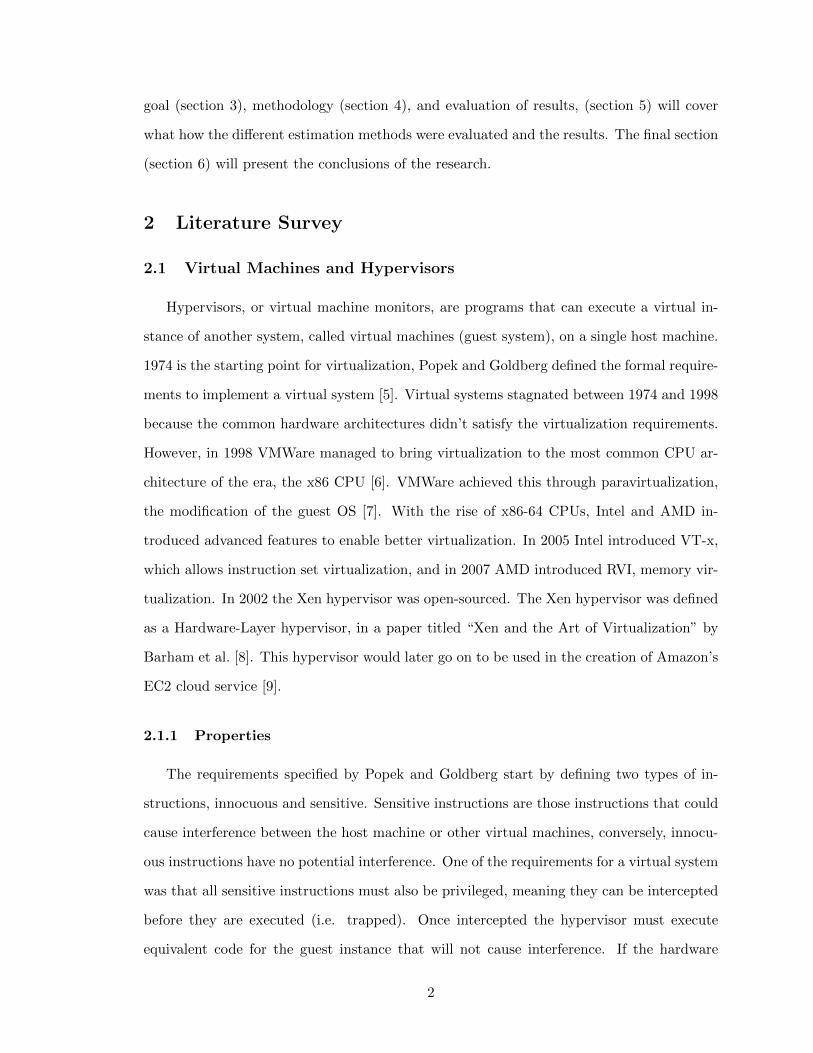
company was created, with the founding of Salesforce.com. The next major milestone for

cloud computing occurred in 2006 when Amazon launched their infrastructure-as-a-service,

the Elastic Compute Cloud [12]. After Amazon launched their cloud service, both Google

and Microsoft followed with their own offerings. A timeline of important events is shown

in figure 2.3.19

95G

rid

com

pu

tin

gis

start

ed

1997

“Clo

ud

Com

pu

tin

g”

coin

ed

1998

VM

Ware

isfo

un

ded

1999

Sal

esfo

rce.

com

isfo

un

ded

2002

Xen

hyp

ervis

or

isop

en-s

ou

rced

2005

Inte

lin

trod

uce

sV

T-x

2006

Am

azon

lau

nch

esE

C2

2007

AM

Din

trod

uce

sR

VI

Figure 2.3. Timeline of important cloud events

What both grid computing and cloud computing tried to achieve is a disruption of the

business model for computation. Before either of these computing models were available,

computational cost was usually a large onetime upfront cost (purchase of the hardware).

However, with these new models the concept of utility computing, paying directly for the

computation time needed, is possible. While both grid computing and cloud computing are

forms of utility computing, there are still differences between their business models.

Grid computing was the earlier concept for utility computing with a focus on large scale

problems. Most grids, such as TeraGrid, were set up in a sharing scheme to solve these large

problems. In this scheme, a group of organizations would join their computational resources

and then allocate them back out from a given criteria. The intention of the sharing was to

increase overall computational capacity by utilizing the downtime of other organization’s

resources [13]. The utility model came from how the resources were allocated by need,

instead of capacity.

Cloud computing was created with a focus on web services, which resulted in a different

6

business model and a different set of features. The biggest difference between the business

models was a change from computation sharing to a pay-as-you-go process. To simplify

the pay-as-you-go model, cloud providers created the following three classifications of cloud

services, which were formalized by National Institute of Standards and Technology(NIST)

[3]:

Infrastructure as a Service (IaaS)

is when access to the hardware resources, or virtualized equivalents, is the product

being sold.

Platform as a Service (PaaS)

is when hosting for user created applications are run on the cloud providers hardware

through their tools and APIs.

Software as a Service (SaaS)

is when the user accesses the cloud provider applications.

NIST also defines 5 essential properties of the cloud as follows [3]:

On-demand Self-service

A user can obtain and allocate computational resources without human intervention.

Broad Network Access

The cloud is readily accessible through standard network mechanisms (usually the

Internet).

Resource Pooling

The provider gathers the computational resources into a pool, wherein consumers can

purchase the resources they need.

Rapid Elasticity

Resources can be acquired and relinquished quickly.

7

Measured Service

Computational resources are monitored, by both the provider and user, in order to

optimize resource control.

For the purposes of this thesis only IaaS will be considered further.

2.2.1 Infrastructure as a Service

To provide Infrastructure as a Service (IaaS), companies such as Amazon, group their

computational resources into instances of various sizes and then sell access to them on an

hourly basis. In order to make the usage of such instances easier, most cloud providers offer

additional management services, such as, load balancing and utilization tracking. These

tools, covered in more detail in sections 2.2.2 and 2.2.3, create a basis for a scalable service.

2.2.2 Instance Management

If a cloud service satisfies NIST requirements, specified in section 2.2, then the user will

have the following tools available to control their utilization of cloud resources:

Utilization Monitor

measures the current resource load of the acquired resources. This will monitor various

aspects of the resources, such as, CPU load, memory usage, network traffic, and

storage usage.

Instance Acquirer

allocates additional resources/instances upon user request.

Instance Relinquisher

deallocates existing resources/instances upon user request.

As a consequence of all of these tools being on-demand self-service, it is possible to

create a scaling function that takes in the current resource utilization and outputs an ex-

pected resource utilization estimate. Once the estimate is generated then the instance

acquirer/relinquisher can adjust the current instance allocation to match the expected uti-

lization. This behavior can be summarized in the following equations 1 and 2.

8

uf = E(uc) (1)

Where,

uc is the current, or recent history, of the utilization of the resources

uf is the estimate of future resource utilization

E is a function that tries to estimate future resource utilization

Ralloc =ufRc

(2)

Where,

uf is the estimate of future resource utilization

Rc is the resource’s computational capacity

Ralloc represents how many instances are needed to serve the expected utilization

2.2.3 Load Balancing Service

To improve the elasticity of their cloud services, several providers which include Google

[14], Amazon [15], and Rackspace [16], have added load balancing as a service. Load

balancers improve a services scalability by distributing the workload evenly across a number

of servers [17]. There are two types of load balancers, content-blind and content-aware.

Content-blind load balancers do not use the purpose of incoming connections when assigning

connections to servers. Conversely, content-aware load balancers do use the purpose of

incoming connections when assigning connections. Content-aware load balancers are only

necessary when the balancer is trying to balance very disparate services into a single set of

servers. However, flash events have been shown to focus on a particular set of homogeneous

resources [18], which would not require content-aware load balancing and therefore only

content-blind load balancers will be covered.

To distribute load to different servers, a load balancer will take in a series of TCP

connections and forward them to a set of servers, hopefully in an equitable manner. For

content-blind forwarding there are three possible solutions for two different network layers.

Additionally, each of these solutions can either be a two-way architecture, meaning the

9

(a) One-way architecture (b) Two-way architecture

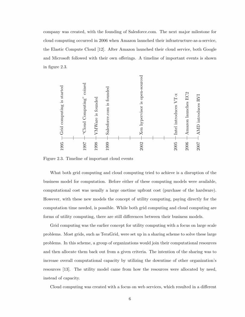
Figure 2.4. Load balancing architectures

returning traffic goes through the load balancer, or one-way architecture, meaning the

returning traffic is sent directly from the loaded servers. The differences in forwarding

architectures are shown in figure 2.4.

Layer-2 forwarding uses direct routing, which places a device between the client-side

(service user) and serve-side (service provider/cloud user) router. This device works by

rewriting the destination MAC address to an internal server, in a way that hides the exis-

tence of an intermediary device while also distributing the connections. Using this forward-

ing method the returning traffic is sent directly from the servers to the service user because

they are all in the same IP subnet (one-way architecture)

Layer-3 forwarding has two different approaches, Network Address Translation (NAT),

which is a two-way architecture, and IP Tunneling, which is a one-way architecture. NAT

works by rewriting the destination address of the incoming, load balanced, and outgoing,

returning packets. This has the potential to make the load balancer a bottleneck in the

system because of the multitude of checksum calculations that need to be performed. The

next method is IP tunneling, which takes the incoming IP datagrams and encapsulates them

in a new datagram that also contains the virtual IP address, the IP address hosting the web

service, and the original source destination. The end-server can then use this information

to directly send the packets back to the service user directly (one-way architecture).

Once a forwarding method is selected, the system must implement a method of distribut-

ing the packets evenly. For content-blind system there are the following four methods:

Round Robin

incoming connections are assigned to servers in a circular manner.

10

Least Connections

an incoming connection is assigned to the server with the least number of connections.

Least Loaded

an incoming connection is assigned to the server with the lowest CPU utilization.

Random

Connections are assigned randomly as they arrive.

There are also weighted versions of the round robin and least connections method that

improve performance when load balancing heterogeneous servers. The least connections

and least loaded methods require additional information tracking that makes them more

costly to implement than the round robin method, at least for homogeneous servers.

2.2.4 Virtual Appliances

Virtual appliances were defined in 2003 by a group of Stanford University researchers as

the combination of a service and its supporting environment that can be executed on a hy-

pervisor [19]. These appliances can either be user generated or offered by the cloud provider.

To reduce the system’s execution and deployment overhead, some virtual appliances have

been built using a new operating system (OS) design called Just Enough Operating Sys-

tem (JeOS, pronounced like juice). By stripping the OS down to just storage, file system,

networking, and support packages, JeOS creates a light and easy to install system with a

small footprint [20]. Lightweight systems help scalability in a number of ways, one of which

is the reduction in startup time. For example, Xiao, Chen, and Luo were able to achieve

70% reduction in an appliance startup time with virtual instances that had only 1 GB of

virtual memory [21]. The startup time was compared against a system going through the

normal boot sequence to one that used the hypervisor’s resume feature.

While not directly related to scaling, virtual appliances are easier to maintain and install

for two reasons. The first reason is because the reduced support environment removes

potential conflicts, which in turn reduces testing time and problems. The second reason

is the virtualization makes setting up additional instances as easy as copy-and-pasting a

11

file. The copy-and-paste nature will also aid the maintenance of a system by easily creating

isolated environments to test software updates/patches.

Overall, virtual appliances offer a way to improve the scaling and maintenance of virtual

instances in a cloud IaaS. Scaling is aided by the lightweight design speeding up start

times and service encapsulation reducing the overhead cost of additional instances. The

encapsulation and lightweight nature also help maintanability by reducing the chance of

problems.

2.3 Flash Events

A flash event is when a large, and possibly unpredicted, number of legitimate users

attempt to access a service concurrently. While large demand for a service could be good

for a business, if the demand starts degrading the response time the business can lose money,

possibly to the extent of 1% sales drop for each 100ms of delay [22]. With a large enough

flash event, websites could become unreachable. Like what happened to the news sites,

CNN and MSNBC, during the 9/11 terrorist attack [23]. Research into flash events has

primarily focused on distinguishing them from distributed denial of service attacks (DDoS).

However, this research is hampered by the lack of traces from real flash events, though a

couple of good traces exist, such as the 1998 FIFA World Cup dataset and the traffic log

for Steve Jobs’ Wikipedia page after his death. From these, and other sources, Bhatia et

al. presented a taxonomy and modeling system for flash events in their paper “Modeling

Web-server Flash Events” [18], which will be covered in more detail in the following sections.

2.3.1 Flash Event Classifications

Before attempting to model flash events, Bhatia et al. divided flash events into the

following three categories:

Predictable Flash Event

the occurrence time of the flash event is known a priori

Unpredictable Flash Event

The occurrence time of the flash event is not known

12

Secondary Flash Event

When a secondary website/service is overloaded by being linked to from a more traf-

ficked website

Figure 2.5. The Slashdot effect

Predictable flash events usually occur when a popular event is scheduled, such as, a

popular product launch or a sporting event. Conversely, unpredictable flash events happen

when the root event is unplanned/unexpected, like the death of a celebrity or a natural

disaster. The last classification is for secondary flash events, which could be considered a

lesser more specific version of an unpredictable flash event. This type of flash event was

given its own classification because of how regularly it happens, in particular, it can go by

another name, “the Slashdoteffect”. What happens is a popular site, such as Slashdot, links

to an under resourced (much less popular) website and the resulting traffic flow overwhelms

linked website). An example of a moderate Slashdot effect is shown in figure 2.5.

2.3.2 Modeling

Bhatia et al. break up a flash event into two separate phases, the flash-phase and the

decay phase. They rejected other flash event models because of the inclusion of a sustained-

traffic phase, which their data showed was magnitudes smaller than the other phases [18].

In figure 2.6 the different phases are illustrated.

For their model, Bhatia et al. created two equations, one equation to model the flash

phase and the other to model the decay-phase. Before creating the equations, Bhatia et al.

13

Figure 2.6. Flash event phases

defined the traffic amplification factor (Af ) as the ratio of the peak rate requests (Rp) to

the average normal request rate (Rn). Af can be set to different values to simulate different

flash event magnitudes. It is also important to mark specific points in the flash event. The

starting point of the flash event is called T0. After that is the flash peak, which will indicate

when the flash-phase will be complete and Rp has been achieved, which is indicated by Tf .

The flash peak also indicates the start of the decay phase, which ends when the request

rate drops back to normal (Rn) and is indicated by Tp.

Flash Phase For the flash-phase they used a standard exponential growth model, which

assumed that increase in the current rate of traffic(dRdt ) was proportional to the current

traffic rate(αR). Such that,

dR

dt= αR

This differential equation can be solved by substituting values from the begining of the

flash event. In particular, t = t0 and R = Rn,

R = Rneα(t−t0) (3)

14

In this equation α is the flash-constant. In order to solve the flash-constant they sub-

stitute values into the equation for when the flash event has reached the peak. This results

in the flash-constant being,

α =lnAf

(tf − T0)

Substituting the flash-constant back into equation 3 they got the following equation that

could model the flash phase of a flash event,

R = RnelnAf

(tf−T0)(t−t0)

(4)

Decay Phase Bhatia et al. used a similar technique to model the decay phase, however,

it was the decrease in traffic that was proportional to the current traffic rate,

dR

dt= −βR

Where, β is the decay-constant. Solving the decay-constant and the differential equation

are similar to what was done for the flash-phase equation (equation 4) and will therefore

be skipped and the final equation presented as follows,

R = Rpe− lnAf(td−Tf )

(t−tf )(5)

With equations 4 and 5, set with parameters Rp, Rn, t0, tf , and tp, it is possible to

model flash events of varying flash peaks, flash-phase lengths, and decay-phase lengths.

Flash Event Data Bhatia et al. gathered data from four flash events across all three

classification. For the predictable flash events they analyzed two events for the 1998 FIFA

World Cup semi-finals. For the unpredictable flash event they used the traffic logs for the

Wikipedia after the death of Steve Jobs. For the last event type, secondary flash event,

they analyzed the traffic to a website experiencing the Slashdot effect. The results of these

analyses is in table 2.1 [21].

15

Table 2.1. Flash event data

Flash Event AmplificationFactor (Af )

NormalRate (Rn)

Peak Rate(Pn)

FlashTime(tf )

DecayTime(td)

FIFA Semi-Final 1st

8.47 1,167,621 9,898,273 3 2

FIFA Semi-Final 2nd

9.47 1,032,715 9,785,128 2 2

Wikipediaafter SteveJobs’ death

582.51 1,826 1,063,665 2 33

Slashdot Ef-fect

78.00 1,000 78,000 2 56

Model Validity The last part of Bhatia et al. modeling effort included validation of their

flash model against real world flash events, in all three classifications. While the results are

too long to list here, overall the model performed well even though it had a slightly faster

flash-phase and a slightly slower decay-phase then the trace data.

2.4 Scaling Framework

For their scaling framework, Vaquero et al. proposed a simple rule framework where

each rule has a specific condition and associated action [24]. The condition must evaluate to

either true or false, and if it evaluates to true then the linked action will be performed. The

potential actions are limited by what the cloud service provides. Potential conditions could

include current demand, budget constraints, and/or whether authorization is granted. For

example, consider the following three rules;

If ((E(uc) > C) AND (I ≥ 8) AND P) Then I++

If ((E(uc) > C) AND (I < 8)) Then I++

If ((E(uc) < C) AND (uc < C) AND (I > 2)) Then I--

Where: I is the number of instances currently running and P indicates if permission

to acquire more instances is granted. The terms E(uc),uc, and C are as covered in section

2.2.2.

16

The rules describe a system that has a total of four properties. The first property is

that there will always be a minimum of two instances allocated. For the second property,

instances will only be released when the expected utilization (E(uc)) and the current uti-

lization (uc) are below the current capacity(C), ideally this is some fraction of the current

capacity to ensure the system is not constantly trying to release instances. The third prop-

erty is that up until eight instances, the system will scale without any human involvement.

The fourth property is that to continue scaling a user must grant permission, this prevents

a cost overrun. The fourth property could be improved with addition of rules that would

report when the system is expected to exceed eight instances.

2.4.1 Scaling Problem

Scaling for a flash event is like trying to solve the problem of how best to keep response

times low without excessive spending. To borrow notation from scheduling algorithms [25],

the problem of response time can be written as a special instance of Total Completion Time

objective function, like follows,

∑Lj (6)

Where: the release date (rj) is the same as the due date (d̄j), ensuring the completion time

(Cj) is greater than the due date, and Lj = Cj − d̄j .

However, equation 6 alone does not capture the monetary constraints, to do this we

must minimize the sum of the usage time of each instance by its hourly cost

∑Ck ∗ ceil(Uk) (7)

Where: k is a unique virtual instance, Ck is the hourly cost of instance k, and Uk is the the

total time the instance executed.

The above equations make the following assumptions:

• The instances are all the same

• The only costs are only from instance execution

17

• An instance is only used once (this is to ensure that Ck ∗ ceil(Uk) is correct)

If both equation 6 and 7 are Minimized, then an optimal solution has been found.

Since the jobs are not known ahead of time an optimal solution cannot be guaranteed, but

heuristic algorithms can be used to allocate instances in an efficient manner.

2.5 Demand Estimation

Scaling for a flash event is essentially trying to satisfy current and expected demand. The

easiest way to satisfy this demand would be to buy as many instances as possible, however,

this would tend to overspend in most circumstances without any benefit. Therefore, the

best way to minimize cost and response time, formally defined in section 2.4, is to accurately

estimate future demand for the service. In the following sections 2.5.1 and 2.5.2, different

methods of estimating demand will be covered.

2.5.1 Current Algorithms

Xiao et al. proposed two methods of estimating demand using the monitorable behavior

of virtual instances, an exponentially weighted moving average (EWMA) and a fast up and

slow down (FUSD) method [4].

The EWMA method, weights the previous expectation (E(t − 1)) against the current

observed demand (O(t)) as follows,

E(t) = α ∗ E(t− 1) + (1− α) ∗O(t), 0 ≤ α ≤ 1 (8)

Values of α closer to 1 will increase responsiveness but lower the stability, while, con-

versely, a value of α closer to 0 will increase stability and lower responsiveness. In their

testing, Xiao et al. found that an α value of 0.7 was nearly ideal. However, this method

has a weakness, in that the current estimation will always be between the previous estimate

and the current observation. In other words, EWMA cannot anticipate increases in de-

mand. The second method, FUSD, was developed to overcome the weakness of EWMA. To

improve the method they allow α to be a negative value, resulting in the following equation,

18

E(t) = O(t) + |α| ∗ (O(t)− E(t− 1)),−1 ≤ α ≤ 0 (9)

This creates an acceleration effect by adding a weighted change from the previous es-

timate to the current observed demand. Their testing also showed an ideal value of -0.2.

This corresponds to the “fast up” part of their algorithm, the next part is meant to prevent

the system from underestimating demand, i.e. “slow down”. In order to slow the fall in

expectation they split the α, depending upon whether the observed demand is increasing

(O(t) > O(t− 1)) or decreasing (O(t) ≤ O(t− 1)), into an increasing α↑ and decreasing α↓.

This results in the following set of equations,

E(t) =

O(t) + |α↑| ∗ (O(t)− E(t− 1)) if O(t) > O(t− 1),−1 ≤ α↑ ≤ 0

α↓ ∗ E(t− 1) + (1− α) ∗O(t) if O(t) ≤ O(t− 1), 0 ≤ α↓ ≤ 1

(10)

The only information still needed to implement these methods is the length of the

measurement window, or more simply the length of the time slice where demand is measured

and averaged into a single value. Larger time slices help reduce the impact noise in the

data at the cost of some responsiveness.

2.5.2 Lead-Lag Filters

Within the control systems field there are a set of filters that behave similar to the

FUSD method, described in section 2.5.1. They are the first order lag filter, first order

lead filter, and second order lead-lag filter. One of the advantages of these filters is their

implementability within real-time systems through discretizations of the Laplace transforms.

I could not find any work related to the usage of lead/lag filters in estimating demand. I did,

however, find work related to transfer functions (the math used to create lead-lag systems)

being used to model short term electrical demand [26], which can experience flash events.

The coverage of these methods will start with the first order lag filter defined by Benoit

Boulet, in chapter 8 of his book ”Fundamentals of signals and systems”, as the following

Laplace transform [27],

19

H(s) =ατs+ 1

τs+ 1(11)

Where τ > 0 and 0 ≤ α < 1

When τ = 0 and the input signal is stable, the filter will decay at a rate equal to e−τx,

where x is the time in seconds. An example of this decay can be seen in figure 2.7 from

time 10s to 20s. The next type of filter is the lead filter, which could be considered a flash

up and flash down method because the filter amplifies changes in the input signal before

following a decay path once the input has stabilized. The Laplace transform for a lead filter

is as follows,

H(s) =ατs+ 1

τs+ 1(12)

Where τ > 0 and α > 1

In this system α controls the amplification of any changes in the input signal. figure

2.7 shows the complete behavior of a lead filter. The last type of filter is a second order

lead-lag filter which combines both the lead filter with the lag filter as follows,

H(s) = K ∗ ατas+ 1

τas+ 1

βτbs+ 1

τbs+ 1(13)

Where τa > 0 and τb > 0 and αa > 1 and 0 ≤ αb < 1

With this the behavior of both first order lead filters and first order lag filters can be

combined to both flash up and slow down. The decaying nature of the filters is comparable to

what Xiao et al. had proposed. Therefore, performance behavior should be similar between

the different methods. One significant advantage that the filters have is the granular control

of both the flash up and slow down phases. This tunability could be used with machine

learning techniques in future work to create systems that adapt to changing flash events.

20

Figure 2.7. Demand estimation comparison.

3 Research Goal

The goal of this research is to show the effectiveness of a lead-lag filter in scaling a

service for a flash event within a cloud environment. To judge the effectiveness of a lead-lag

filter’s ability to anticipate demand, this method will be compared to methods proposed by

Xiao et al. The algorithms will be primarily judged by response time and resource cost, as

covered in section 2.4.1.

4 Methodology

The three methods for estimating future demand EWMA, FUSD, and lead/lag filters,

as covered in section 2.5, will be implemented and compared in a scalable test environment.

This environment will have a custom load balancer that can handle the addition and removal

of virtual instances. The estimation methods will be combined with scaling rules similar

to what was presented in section 2.4. The flash event model presented in section 2.3.2 will

be used to generate flash events for the implementations to handle. This traffic will then

be routed through the load balancer to custom virtual appliances, as described in section

2.2.4, that will handle the execution of tasks.

21

4.1 Test Environment

The test environment contains four primary components; tasks, the traffic generator,

the load balancer, and the worker nodes. The hardware for the traffic generator, load

balancer, and the worker nodes is given in table 4.1. The load balancer and worker nodes

are all virtual instances running running on separate hardware, i.e. one machine for the

load balancer and eight different machines for the worker nodes. The traffic generator is

not running in a virtual instance but is on an isolated machine.

Table 4.1. Test hardware

CPU CPUSpeed(Ghz)

Cores/Threads

MemoryCapacity(GB)

MemorySpeed(Mhz)

Virtual

WorkerNode

Intel XeonE3-1270 v2

3.5 4 / 8 4 1600 Yes

LoadBalancer

Intel XeonE3-1270 v2

3.5 4 / 8 4 1600 Yes

TrafficGenerator

Intel Corei5-3570

3.4 4 / 4 16 1600 No

The traffic generator is responsible for creating tasks at a rate given by the flash model

specified in section 4.2. The traffic generator is also responsible for receiving tasks after

they’ve finished execution for analysis of response times. Once a task is created it is then

sent to the load balancer, which will forward the tasks to the worker nodes using a round

robin algorithm. However, the load balancer’s primary task is to apply the scaling rules

specified in section . To apply these rules the load balancer will have the ability to poll all

worker nodes to collect CPU utilization data, shutdown worker nodes to remove instances,

and start the nodes when adding instances. The load balancer will also track when instances

are started and stopped for analysis. Once a task arrives at the worker node it is placed in

a queue for processing. Each worker node has eight threads dedicated to the execution of

tasks. Once a task is finished executing it is sent back to the traffic generator for analysis.

There are in total eight worker nodes that can work on executing tasks. Figure 4.1 shows

how the tasks flow through the test environment.

To allow the traffic generator to overcome an at least eight to one computational advan-

tage of the worker nodes, each task is implemented to require 1s to execute. Tasks record

22

Figure 4.1. The testing environment

information on creation time, execution start time, the time they are sent back to the traffic

generator, and when the arrive at the traffic generator. The creation time and execution

time are used to calculate the response time of each task. Differences between the worker

nodes and the traffic generator system clock could skew the results by either inflating or

minimizing the actual start time. To prevent this skewing the tasks adjust the response time

by reducing it by the difference between the sent time and the arrival time. This works by

reducing the response time if the worker node’s clock is greater than the traffic generator’s

clock and conversely increasing it if the worker node is behind the traffic generator’s clock.

Completion time is not tracked because each task is executed in a non-preemptive manner,

this guarantees that each task will complete 1s after it is started.

4.2 Flash Event Model

To implement the flash model specified in section 2.3.2 the request rates will be changed

to percentage capacity of a single worker node, where 100% indicates complete utilization

of a single worker. For example, if six worker nodes are active with 80% utilization the

percentage capacity would be 480%. With this scheme it easier to model flash events within

the limited capacity of the test environment without exceeding capacity, which can obscure

differences between the different estimation techniques. The test environment cannot handle

modeling amplification factor greater than 120, which means only a predicted flash event

and a secondary flash event can be handled. Data from table 2.1 is used to generate the

following parameters (table 4.2) for the two flash event models.

23

Table 4.2. Flash events for testing

FlashEventType

AmplificationFactor

NormalTraffic(%)

PeakTraffic(%)

FlashTime(minutes)

DecayTime(Minutes)

Predicted 10 64 640 30 30

Secondary 80 8 640 15 420

4.3 Scaling Rules

Each scaling method will implement the following four rules:

1. Add instance when anticipated demand is greater than 90% of current capacity

2. Remove instance only if the removal will not increase demand above 85%

3. Total instances will not exceed 8

4. Total instances will not decrease below 1

All aspects but the demand estimation will be held constant to ensure that the results

between different tests can properly show the effects of demand estimation.

4.4 Demand Estimation Techniques

The following five techniques will be implemented to determine the performance of

lead/lag filters.

Current Demand

Control method to test how the scaling rules work without anticipation

Exponentially Weighted Moving Average (EWMA)

A method that lags the current demand

Flash-Up Slow-Down (FUSD)

Demand anticipation method proposed by Xiao et al.

First-Order Lead Filter

The maximum between the current demand a lead filter specified by equation 14

24

Second-Order Lead-Lag Filter

A second order lead-lag filter specified by equation 15

The first and second order filters are given by the following equations,

1.2s+ 1

s+ 1(14)

The above equation uses the same lead characteristic as the FUSD method with an

overshoot on a transient of 1.2. This method uses the maximum between the current demand

and the output of lead filter to ensure that the anticipated demand doesn’t undershoot

causing a loss in responsiveness.

1.26s2 + 2.5s+ 1

s2 + 2s+ 1(15)

The above filter was designed to combine both the lead and lag qualities of the FUSD

method in a single filter. Figure 4.2 shows an example of the above filters responding to a

simple demand model.

Figure 4.2. Demand response example

25

4.5 Test Phases

Traffic will be generated in four phases; the start up phase, the flash phase, the decay

phase, and the normalization phase. The start up phase will be 1 minute long where demand

generated will correspond to the normal rate. In this phase the load balancer will manually

adjust the instance capacity to be optimal. The goal of this phase is to get the system

into a steady state before the flash event starts. Therefore, data for this phase will not

be collected. The next two phases, flash and decay, will generate demand according to the

flash model specified in section 4.2. The last phase, normalization, is meant to measure

how long the system takes to return to optimal capacity from any over-provisioning.

4.6 Limitation

While running the flash event the actual demand lagged behind the generated demand.

To quantify this inaccuracy, a scenario was created where the demand will rise every five

minutes by 5% from 0% demand to 115% demand. Scaling rules were disabled to ensure a

second instance did not affect the results. The utilization rate is measured once a minute

giving five utilization rate data points per generated demand rate. However, the first and

last data points are excluded because they may include the transition from one demand

rate to another. The results of this test are in figure 4.3. In short, the actual demand was

about 80% of the generated demand.

The tests are also limited by a lack of variability, i.e. noise, in the generated demand. A

lack of noise would benefit methods more inclined to remove a worker instance, such as, the

lead filter and the lea-lag filter. Adding variability to the flash model would require further

research into how users access a service. This is beyond the current scope of research and

will only be mentioned.

26

Figure 4.3. Generated demand inaccuracy

5 Evaluation of results

5.1 Allocation Graphs

The following figures show how each scaling method allocates capacity based upon the

scaled demand. 100% demand indicates that one worker node is fully utilized (as described

in section 4.2). Demand was measured by how many tasks where sent per second filtered

through a 5 second rolling average. Capacity is calculated by measuring how many instances

where active at any given time. The graphs are not adjusted to account for the inaccuracy

in the actual demand. Some of the below charts show temporary drops in demand, con-

sidering the fact that some of the demand estimation methods responded to these drops it

is reasonable to conclude that the drop in demand is real. The root cause of these drops

is unknown, however, the drop is consistent across tests and should not interfere with the

results.

27

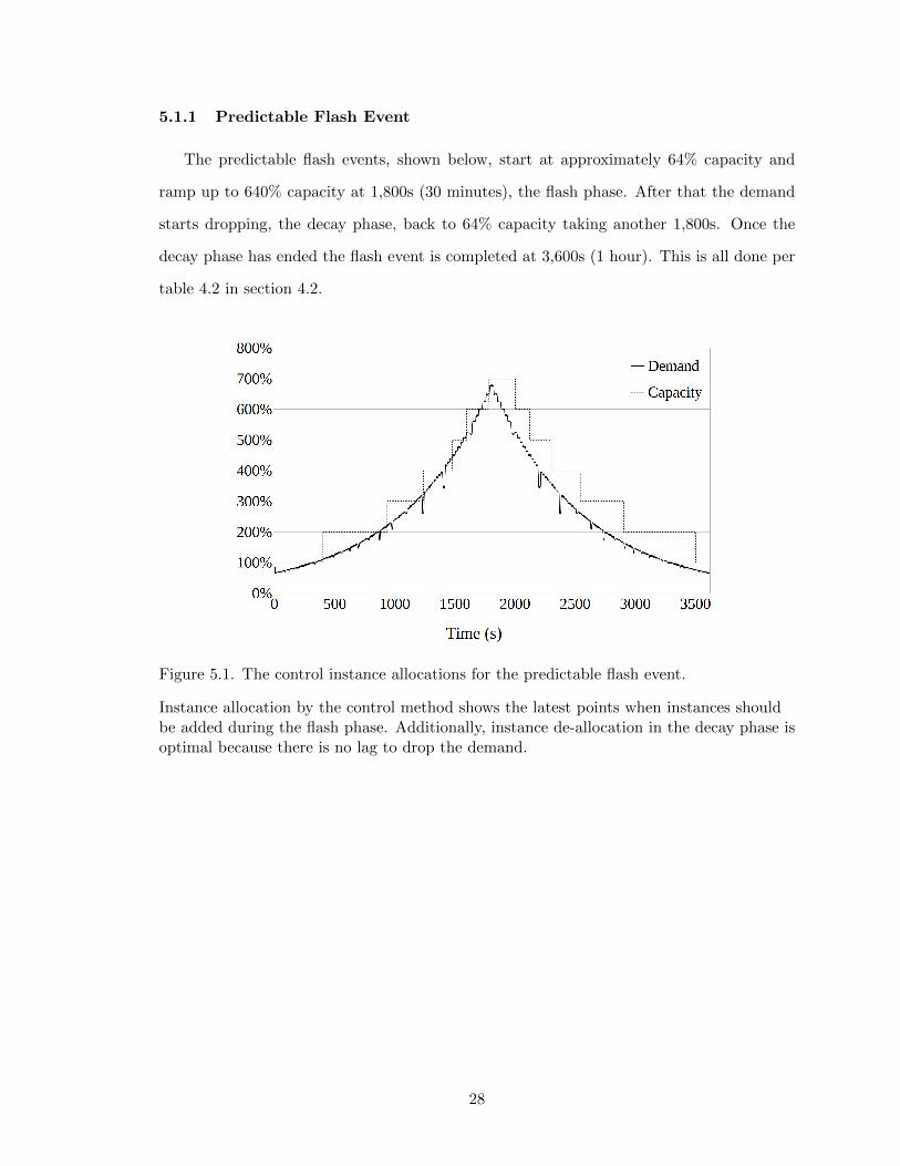
5.1.1 Predictable Flash Event

The predictable flash events, shown below, start at approximately 64% capacity and

ramp up to 640% capacity at 1,800s (30 minutes), the flash phase. After that the demand

starts dropping, the decay phase, back to 64% capacity taking another 1,800s. Once the

decay phase has ended the flash event is completed at 3,600s (1 hour). This is all done per

table 4.2 in section 4.2.

Figure 5.1. The control instance allocations for the predictable flash event.

Instance allocation by the control method shows the latest points when instances shouldbe added during the flash phase. Additionally, instance de-allocation in the decay phase isoptimal because there is no lag to drop the demand.

28

Figure 5.2. The EWMA instance allocations for the predictable flash event.

The EWMA method allocates instances after the control method creating the potentialfor a loss in responsiveness from under provisioning. Furthermore, the the decay phase isover provisioned because of the EWMA lag.

Figure 5.3. The FUSD instance allocations for the predictable flash event.

The FUSD leads the control method during the flash, which help increase taskresponsiveness. However, the FUSD method, like EWMA method, over provisions duringthe flash phase. Although this over provisioning could aid responsiveness if the generateddemand was more random.

29

Figure 5.4. The lead filter instance allocations for the predictable flash event.

The lead filter performs similarly to the FUSD method during the flash phase but doesn’tsuffer the same over provisioning. In particular, during the decay phase, the lead filterperforms comparably to the control method.

Figure 5.5. The lead-lag instance allocations for the predictable flash event.

The lead-lag filter leads the demand like the FUSD and lead filter methods to helpincrease responsiveness. However, during the decay phase the instances are de-allocatedsooner then the control method, and even the lead filter. This could reduce the instancecost at a possible loss of responsiveness.

30

5.1.2 Secondary Flash Event

The secondary flash events, shown below, starts at approximately 8% capacity and

ramps up to 640% capacity at 900s (15 minutes), the flash phase. After this demand starts

dropping, the decay phase, back to 8% capacity in 25,200s (7 hours), which ends the flash

event at 26,100s (7 hours and 15 minutes). This is all done per table 4.2 in section 4.2.

Figure 5.6. The control instance allocations for the secondary flash event.

The control method will again set the standard to judge the other methods. The onlydifference with this flash event is the time it takes to ramp up to peak demand is half thetime used in the predictable flash event, which caused effect discussed more in section 5.3.

31

Figure 5.7. The EWMA instance allocations for the secondary flash event.

The EWMA method performed much as it did in the predictable flash event by underprovisioning in the flash phase and over provisioning in the decay phase.

Figure 5.8. The FUSD instance allocations for the secondary flash event.

The FUSD method did not perform as well in the secondary flash event compared to thepredictable flash event because of the quicker flash phase. Although it still outperformedthe control method by allocating instances sooner.

32

Figure 5.9. The lead filter instance allocations for the secondary flash event.

The lead filter outperformed the FUSD method by allocating and de-allocating instancesearlier. This could produce a lower response time with an overall lower cost.

Figure 5.10. The lead-lag filter instance allocations for the secondary flash event.

The lead-lag filter outperformed the FUSD method and the lead filter by allocating andde-allocating instances earlier. This could produce a slightly lower response time with aslightly lower cost.

33

5.2 Cost

Table 5.1 normalized the cost, measured by total instance time, of each run to the

percent improvement over the control.

Table 5.1. Cost results

EWMA FUSD LeadFilter

Lead-LagFilter

Predicted 0.94% -10.6% -2.1% -0.6%

Secondary 3.25% -2.4% -1.2% 0.4%

The EWMA method consistently came under the cost of the control. The only other

method to beat the control was the lead-lag filter during the secondary flash event, although

overall the lead-lag generated costs similar to the control event. Additionally, both the lead

filter and the lead-lag filter had lower costs than the FUSD method.

5.3 Responsiveness

Responsiveness was measured as the average of the 1% highest response times, this was

done to reduce the chance a single bad response to skew the results. Table 5.2 normalizes the

results to the percent improvement over the control. The responsiveness of the secondary

flash event was much worse than the predictable flash event, 9ms vs 4.3s in the control

method, which caused the lead and lead-lag filters to perform better than the FUSD method.

Table 5.2. Responsiveness results

EWMA FUSD LeadFilter

Lead-LagFilter

Predicted -99% 232.6% 43.7% 55.9%

Secondary -99% 40.8% 2,937% 31,251%

The EWMA method created response times over 100 times slower than any other method

making it an unsuitable method for handling a flash event. Both the lead filter and the

lead-lag filter showed the most improvement over the control in the secondary flash because

flash rate accelerated much faster than the predictable flash event. However, in the slower

accelerating predictable flash event the FUSD had the advantage in responsiveness.

34

6 Conclusion

This thesis covered the history of virtualization, from 1973’s Popek and Goldberg re-

quirements to the introduction of x86-64 virtualization extensions in mid-2000. More im-

portantly, virtualization made cloud services elastic, i.e. malleable for a range of users

needs, by providing an abstraction of the physical hardware. Some cloud providers, such as

Google, offer a load balancing service to evenly spread demand across a series of resource

instances. Load balancing services improves cloud elasticity by distributing incoming con-

nections evenly across any active resource instances. This elasticity makes the cloud better

at responding to changes in demand rather than purchasing and using physical hardware.

Changes in demand occur in many ways, from user growth to increased service usage

from current users. However, there is a special type of change in demand, a flash event,

that happens so quickly that it can degrade a web services ability to operate. A flash event

is where the demand for a service rapidly increases over a very brief period of time, usually

just hours, to possibly over a 100 times the normal traffic rate. There are three common

varieties of flash events; predictable, unpredictable, and secondary. Flash events cause

problems when demand outstrips the underlying resources causing a drop in response time,

which Amazon found can cause a 1% drop in sales for every 100ms of increased response

time [22].

Scaling for a flash event requires the anticipation of future demand because of the time

it takes to allocate additional resources; this can range from a couple of seconds to minutes.

This thesis focused on the usage of lead/lag filters, which are Laplace domain equations that

can be tuned to over and/or under shoot demand. To fully evaluate the effectiveness of

lead-lag filters in anticipating demand they were compared against the leading method from

Xiao, et al. the flash-up slow-down method (FUSD). Whatever the anticipation method it

must be coupled with a set of scaling rules to ensure that the instances are allocated and

de-allocated only when intended.

In order to test these estimation methods a testing environment was created to simulate

an Infrastructure as a Service. This environment contained a load balancer and eight worker

nodes to handle traffic. Generated traffic was created in accordance with the flash event

35

model from Bhatia, et al, that uses tasks to create measurable CPU load. This CPU load

is then used during the flash event to approximate demand for the estimation method and

scaling rules. Only the predictable and secondary flash events were tested in the environment

due to resource limitations.

The results of this testing showed that the lowest cost estimation method was EWMA,

but this produced a response time that was magnitudes worse than any other methods.

The lead-lag filter estimation method had the next lowest cost by around 1% of the control.

This lower cost, however, didn’t come at a worsened response time over the lead filter

estimation method and actually beat the competitor algorithm, FUSD, in the secondary

flash event. The lead filter did not perform as well as the lead-lag filter in terms of cost or

responsiveness but still outperformed the FUSD method in cost and, for only the secondary

flash event, responsiveness. These results may not hold if the generated demand was noisier.

In conclusion, first and second order filters can improve responsiveness at a slight cost over

a direct method of measuring demand. Furthermore, the filters are an improvement over

the lead competitor’s algorithm, FUSD, in cost and are better at handling the rapidly

accelerating demand of a secondary flash event.

36

References

[1] D. Rushe, “Steve jobs, apple co-founder, dies at 56,” Oct. 2011,

http://www.guardian.co.uk/technology/2011/oct/06/steve-jobs-apple-cofounder-

dies.

[2] D. Woodside, “We owe you an apology,” Dec. 2013, http://motorola-

blog.blogspot.com/2013/12/we-owe-you-apology.html.

[3] P. Mell and T. Grance, “The nist definition of cloud computing: Recommendations of

the national institute of standards and technology,” Sep. 2011.

[4] Z. Xiao, W. Song, and Q. Chen, “Dynamic resource allocation using virtual machines

for cloud computing environment,” Parallel and Distributed Systems, IEEE Transac-

tions on, vol. 24, no. 6, pp. 1107–1117, June 2013.

[5] G. J. Popek and R. P. Goldberg, “Formal requirements for virtualizable third genera-

tion architectures,” in Proceedings of the Fourth ACM Symposium on Operating System

Principles, ser. SOSP ’73. New York, NY, USA: ACM, 1973, pp. 121–, http://0-

doi.acm.org.opac.library.csupomona.edu/10.1145/800009.808061.

[6] O. Agesen, A. Garthwaite, J. Sheldon, and P. Subrahmanyam, “The evolution of an

x86 virtual machine monitor,” SIGOPS Oper. Syst. Rev., vol. 44, no. 4, pp. 3–18, Dec.

2010, http://0-doi.acm.org.opac.library.csupomona.edu/10.1145/1899928.1899930.

[7] E. Bugnion, S. Devine, M. Rosenblum, J. Sugerman, and E. Y. Wang, “Bring-

ing virtualization to the x86 architecture with the original vmware workstation,”

ACM Trans. Comput. Syst., vol. 30, no. 4, pp. 12:1–12:51, Nov. 2012, http://0-

doi.acm.org.opac.library.csupomona.edu/10.1145/2382553.2382554.

[8] P. Barham, B. Dragovic, K. Fraser, S. Hand, T. Harris, A. Ho, R. Neuge-

bauer, I. Pratt, and A. Warfield, “Xen and the art of virtualization,”

SIGOPS Oper. Syst. Rev., vol. 37, no. 5, pp. 164–177, Oct. 2003, http://0-

doi.acm.org.opac.library.csupomona.edu/10.1145/1165389.945462.

37

[9] J. Bezos, “Amazon ec2 beta,” Aug. 2006, http://aws.typepad.com/aws/2006/08/amazon ec2 beta.html.

[10] J. Sahoo, S. Mohapatra, and R. Lath, “Virtualization: A survey on concepts, taxonomy

and associated security issues,” in Computer and Network Technology (ICCNT), 2010

Second International Conference on, April 2010, pp. 222–226.

[11] X. Project, “Xen 4.3 release notes,” Jul. 2013,

http://wiki.xenproject.org/wiki/Xen 4.3 Release Notes (Accessed on March 3,

2014).

[12] G. Staff, “30 years of accumulation: a timeline of cloud cimputing,” Mar. 2013,

http://gcn.com/articles/2013/05/30/gcn30-timeline-cloud.aspx (Accessed on March 3,

2014).

[13] I. Foster, Y. Zhao, I. Raicu, and S. Lu, “Cloud computing and grid computing 360-

degree compared,” in Grid Computing Environments Workshop, 2008. GCE ’08, nov

2008, pp. 1–10.

[14] Google, “Load balancing,” Mar. 2014, https://developers.google.com/compute/docs/load-

balancing/ (Accessed on March 4, 2014).

[15] Amazon, “Elastic load balancing,” Mar. 2014, http://aws.amazon.com/elasticloadbalancing/

(Accessed on March 3, 2014).

[16] Rackspace, “Load balancing as a service,” Mar. 2014,

http://www.rackspace.com/cloud/load-balancing/ (Accessed on March 3, 2014).

[17] K. Gilly, C. Juiz, and R. Puigjaner, “An up-to-date survey in web load

balancing,” World Wide Web, vol. 14, no. 2, pp. 105–131, 2011. [Online]. Available:

http://dx.doi.org/10.1007/s11280-010-0101-5

[18] S. Bhatia, G. Mohay, D. Schmidt, and A. Tickle, “Modelling web-server flash events,”

in Network Computing and Applications (NCA), 2012 11th IEEE International Sym-

posium on, Aug 2012, pp. 79–86.

38

[19] C. Sapuntzakis, D. Brumley, R. Chandra, N. Zeldovich, J. Chow, M. S. Lam,

and M. Rosenblum, “Virtual appliances for deploying and maintaining software,” in

Proceedings of the 17th USENIX Conference on System Administration, ser. LISA ’03.

Berkeley, CA, USA: USENIX Association, 2003, pp. 181–194. [Online]. Available:

http://dl.acm.org/citation.cfm?id=1051937.1051965

[20] D. Geer, “The os faces a brave new world,” Computer, vol. 42, no. 10, pp. 15–17, Oct

2009.

[21] Z. Xiao, Q. Chen, and H. Luo, “Automatic scaling of internet applications for cloud

computing services,” IEEE Transactions on Computers, vol. 99, no. PrePrints, p. 1,

2012.

[22] G. Linden, “Make data useful,” Nov. 2006, amazon, Presentation.

[23] J. Hu and G. Sandoval, “Web acts as hub for info on attacks,” Sep. 2001, accessed

http://news.cnet.com/2100-1023-272873.html on March 3, 2014.

[24] L. M. Vaquero, L. Rodero-Merino, and R. Buyya, “Dynamically scaling applications in

the cloud,” SIGCOMM Comput. Commun. Rev., vol. 41, no. 1, pp. 45–52, Jan. 2011,

http://0-doi.acm.org.opac.library.csupomona.edu/10.1145/1925861.1925869.

[25] J. Leung, Handbook of scheduling : algorithms, models, and performance analysis.

Boca Raton: Chapman & Hall/CRC, 2004.

[26] F. J. Nogales and A. J. Conejo, “Electricity price forecasting through transfer

function models,” The Journal of the Operational Research Society, vol. 57,

no. 4, pp. 350–356, 04 2006, copyright - Palgrave Macmillan Ltd 2006;

Last updated - 2013-10-04; CODEN - OPRQAK. [Online]. Available: http:

//search.proquest.com/docview/231377045?accountid=10357

[27] B. Boulet, Fundamentals of signals and systems. Hingham, Mass: Da Vinci Engineer-

ing Press, 2006.

39