LLNL-JRNL-479591

Scaling hypre's multigrid solversto 100,000 cores

A. H. Baker, R. D. Falgout, T. V. Kolev, U. M.Yang

April 8, 2011

High Performance Scientific Computing: Algorithms andApplications

Disclaimer

This document was prepared as an account of work sponsored by an agency of the United States government. Neither the United States government nor Lawrence Livermore National Security, LLC, nor any of their employees makes any warranty, expressed or implied, or assumes any legal liability or responsibility for the accuracy, completeness, or usefulness of any information, apparatus, product, or process disclosed, or represents that its use would not infringe privately owned rights. Reference herein to any specific commercial product, process, or service by trade name, trademark, manufacturer, or otherwise does not necessarily constitute or imply its endorsement, recommendation, or favoring by the United States government or Lawrence Livermore National Security, LLC. The views and opinions of authors expressed herein do not necessarily state or reflect those of the United States government or Lawrence Livermore National Security, LLC, and shall not be used for advertising or product endorsement purposes.

Scaling hypre’s multigrid solvers to 100,000cores

Allison H. Baker, Robert D. Falgout, Tzanio V. Kolev, and Ulrike Meier Yang

Abstract Thehypre software library [15] is a collection of high performance pre-conditioners and solvers for large sparse linear systems of equations on massivelyparallel machines. This paper investigates the scaling properties of several of thepopular multigrid solvers and system building interfaces inhypre on two modernparallel platforms. We present scaling results on over 100,000 cores and even solvea problem with over a trillion unknowns.

1 Introduction

The need to solve increasingly large, sparse linear systems of equations on parallelcomputers is ubiquitous in scientific computing. Such systems arise in the numeri-cal simulation codes of a diverse range of phenomena, including stellar evolution,groundwater flow, fusion plasmas, explosions, fluid pressures in the human eye, andmany more. Generally these systems are solved with iterative linear solvers, suchas the conjugate gradient method, combined with suitable preconditioners, see e.g.[17, 19].

A particular challenge for parallel linear solver algorithms is scalability. An ap-plication code is scalable if it can use additional computational resources effectively.In particular, in this paper we focus onweak scalability, which requires that if thesize of a problem and the number of cores are increased proportionally, the comput-ing time should remain approximately the same. Unfortunately, in practice, as sim-ulations grow to be more realistic and detailed, computing time may increase dra-matically even when more cores are added to solve the problem. Recent machines

Allison Baker· Rob Falgout· Tzanio Kolev· Ulrike YangLawrence Livermore National Laboratory, Center for Applied Scientific Computing, e-mail:{abaker,rfalgout,tzanio,umyang}@llnl.gov.This work performed under the auspices of the U.S. Department of Energy by Lawrence LivermoreNational Laboratory under Contract DE-AC52-07NA27344 (LLNL-JRNL-479591).

1

2 Baker,Falgout,Kolev,Yang

with tens or even hundreds of thousands of cores offer both enormous computingpossibilities and unprecedented challenges for achieving scalability.

The hypre library was developed with the specific goal of providing users withadvanced parallel linear solvers and preconditioners that are scalable on massivelyparallel architectures. Scalable algorithms are essential for combating growing com-puting times. The library features parallel multigrid solvers for both structuredand unstructured problems. Multigrid solvers are attractive for parallel computingbecause of their scalable convergence properties. In particular, if they are well-designed, then the computational cost depends linearly on the problem size, andincreasingly larger problems can be solved on (proportionally) increasingly largernumbers of cores with approximately the same number of iterations to solution. Thisnatural algorithmic scalability of the multigrid methods combined with the robustand efficient parallel algorithm implementations inhypre result in preconditionersthat are well-suited for large numbers of cores.

Thehypre library is a vital component of a broad array of application codes bothat and outside of Lawrence Livermore National Laboratory (LLNL). For example,the library was downloaded more than 1800 times from 42 countries in 2010 alone,approaching nearly 10,000 total downloads from 70 countries since its first opensource release in September of 2000. The scalability of its multigrid solvers hasa large impact on many applications, particularly because simulation codes oftenspend the majority of their runtime in the linear solve.

The objective of this paper is to demonstrate the scalability of the most popu-lar multigrid solvers inhypre on current supercomputers. We present scaling stud-ies for conjugate gradient, preconditioned with the structured-grid solvers PFMG,SMG, SysPFMG, as well as the algebraic solver BoomerAMG, and the unstructuredMaxwell solver AMS. Note that previous investigations beyond 100,000 cores fo-cused only on the scalability of BoomerAMG on various architectures and can befound in [5, 2].

The paper is organized as follows. First we provide more details about the overallhypre library in Section 2 and the considered multigrid linear solvers in Section 3.Next, in Section 4, we specify the machines and the test problems we used in ourexperimental setup. We present and discuss the corresponding scalability results inSection 5, and we conclude by summarizing our findings in Section 6.

2 The hypre library

In this section we give a general overview of thehypre library. More detailed infor-mation can be found in the User’s Manual available on thehypre web page [15].

Scaling hypre’s solvers to 100,000 cores 3

2.1 Conceptual interfaces

We first discuss three of the so-calledconceptual interfacesin hypre, that providedifferent mechanisms for describing a linear system on a parallel machine. These in-terfaces not only facilitate the use of the library, but they make it possible to providelinear solvers that take advantage of additional information about the application.

TheStructured Grid Interface (Struct ) is a stencil-based interface that is mostappropriate for scalar finite-difference applications whose grids consist of unions oflogically rectangular (sub)grids. The user defines the matrix and right-hand side interms of the stencil and the grid coordinates. This geometric description, for exam-ple, allows the use of the PFMG solver, a parallel algebraic multigrid solver withgeometric coarsening, described in more detail in the next section.

The Semi-Structured Grid Interface (SStruct ) is essentially an extension ofthe Structured Grid Interface that can accommodate problems that are mostly struc-tured, but have some unstructured features (e.g., block-structured, composite oroverset grids). It can also accommodate multiple variables and variable types (e.g.,cell-centered, edge-centered, etc.), which allows for the solution of more generalproblems. This interface requires the user to describe the problem in terms of struc-tured gridparts, and then describe the relationship between the data in each partusing either stencils or finite element stiffness matrices.

TheLinear-algebraic Interface (IJ ) is a standard linear-algebraic interface thatrequires that the users map the discretization of their equations into row-columnentries in a matrix structure. Matrices are assumed to be distributed acrossP MPItasks in contiguous blocks of rows. In each task, the matrix block is split into twocomponents which are each stored in compressed sparse row (CSR) format. Onecomponent contains the coefficients that are local to the task, and the second, whichis generally much smaller than the local one, contains the coefficients whose col-umn indices point to rows located in other tasks. More details of the parallel matrixstructure, called ParCSR, can be found in [10].

2.2 Solvers

Thehypre library contains highly efficient and scalable specialized solvers as wellas more general-purpose solvers that are well-suited for a variety of applications.

The specialized multigrid solvers use more than just the matrix to solve cer-tain classes of problems, a distinct advantage provided by the conceptual interfaces.For example, the structured multigrid solvers SMG, PFMG, and SysPFMG all takeadvantage of the structure of the problem. As a result, these solves are typicallymore efficient and scalable than a general-purpose solver alternative. The SMG andPFMG solvers require the use of theStruct interface, and SysPFMG requires theSStruct interface.

For electromagnetic problems,hypre provides the unstructured Maxwell solver,AMS, which is the first provably scalable solver for definite electromagnetic prob-

4 Baker,Falgout,Kolev,Yang

lems on general unstructured meshes. The AMS solver requires matrix coefficientsplus the discrete gradient matrix and the vertex coordinates which can be describedwith the IJ or SStruct interface.

For problems on arbitrary unstructured grids,hypre provides a robust parallelimplementation of algebraic multigrid (AMG), called BoomerAMG. BoomerAMGcan be used with any interface (currently not supported throughStruct ), as it onlyrequires the matrix coefficient information.

Thehypre library also provides common general-purpose iterative solvers, suchas the GMRES and Conjugate Gradient (CG) methods. While these algorithms arenot scalable as stand-alone solvers, they are particularly effective (and scalable)when used in combination with a scalable multigrid preconditioner.

2.3 Considerations for large-scale computing

Several features of thehypre library are required to efficiently solve very large prob-lems on current supercomputers. Here we describe three of these features: supportfor 64-bit integers, scalable interface support for large numbers of MPI tasks, andthe use of a hybrid programming model.

64-bit integer support has recently been added inhypre. This support is neededto solve problems in ParCSR format with more than 2 billion unknowns (previouslya limitation due to 32-bit integers). To enable the 64-bit integer support,hypre mustbe configured with the--enable-bigint option. When this feature is turned on,the user must passhypre integers of typeHYPREInt , which is the 64-bit integer(usually a ’long long int’ type in C). Note that this 64-bit integer option converts allintegers to 64-bit, which does affect performance and increases memory use.

Scalable interfacesas well as solver algorithms are required for a code utilizinghypre to be scalable. When using one ofhypre’s interfaces, the problem data ispassed tohypre in its distributed form. However, to obtain a solution via a multigridmethod or any other linear solver algorithm, MPI tasks need to obtain nearby datafrom other tasks. For a task to determine which tasks own the data that it needs, i.e.their communication partners or neighbors, some information regarding the globaldistribution of the data is required. Storing and querying a global description of thedata, which is the information detailing which MPI task owns what data or theglobalpartition, is either too costly or not possible when dealing with tens of thousands ormore tasks. Therefore, to determine inter-task communication in a scalable manner,we developed new algorithms that employ anassumed partitionto answer queriesthrough a type of rendezvous algorithm, instead of storing global data descriptions.This strategy significantly reduces storage, communication, and computational costsfor the solvers inhypre and improves scalability as shown in [4]. Note that thisoptimization requires configuringhypre with the --no-global-partition optionand is most beneficial when using tens of thousands of tasks.

A hybrid programming model is used inhypre. While we have obtained goodscaling results in the past using an MPI-only programming model, see e.g. [11],

Scaling hypre’s solvers to 100,000 cores 5

with increasing numbers of cores per node on multicore architectures, the MPI-onlymodel is expected to be increasingly insufficient due to the limited off-node band-width and decreasing amounts of memory per core. Therefore, inhypre we alsoemploy a mixed or hybrid programming model which combines both MPI and theshared memory programming model OpenMP. The OpenMP code inhypre is largelyused in loops and divides a loop amongk threads into roughlyk equal-sized portions.Therefore, basic matrix and vector operations, such as the matrix-vector multiply ordot product, are straightforward, but the use of OpenMP within other more complexparts of the multigrid solver algorithm, such as in parts of the setup phase (de-scribed in Section 3), may be non-trivial. The right choice for hybrid MPI/OpenMPpartitioning in terms of obtaining optimal performance is dependent on the specifictarget machine’s node architecture, interconnect, and operating system capabilities[5]. See [5] or [2] for more discussion on the performance of BoomerAMG with ahybrid programming model.

3 The multigrid solvers

As mentioned in Section 1, multigrid solvers are algorithmically scalable, mean-ing that they require O(N) computations to solve a linear system withN variables.This desirable property is obtained by cleverly utilizing a sequence of smaller (orcoarser) grids, which are computationally cheaper to compute on than the original(finest) grid. A multigrid method works as follows. At each grid level, a smoother isapplied to the system, which serves to resolve the high-frequency error on that level.The improved guess is then transferred to a smaller, or coarser, grid, the smootheris applied again, and the process continues. The coarsest level is generally chosento be a size that is reasonable to solve directly, and the goal is to eliminate a signif-icant part of the error by the time this coarsest level is reached. The solution to thecoarse grid solve is then interpolated, level by level, back up to the finest grid level,applying the smoother again at each level. A simple cycle down and up the grid isreferred to as a V-cycle. To obtain good convergence, the smoother and the coarse-grid correction process must complement each other to remove all components ofthe error.

A multigrid method has two phases: the setup phase and the solve phase. Thesetup phase consists of defining the coarse grids, interpolation operators, and coarse-grid operators for each of the coarse-grid levels. The solve phase consists of per-forming the multilevel cycles (i.e., iterations) until the desired convergence is ob-tained. In the scaling studies, we often time the setup phase and solve phase sep-arately. Note that while multigrid methods may be used as linear solvers, they aremore typically used as preconditioners for Krylov methods such as GMRES or con-jugate gradient.

The challenge for multigrid methods on supercomputers is turning an efficientserial algorithm into a robust and scalable parallel algorithm. Good numerical prop-erties need to be preserved when making algorithmic changes needed for paral-

6 Baker,Falgout,Kolev,Yang

lelism. This non-trivial task affects all aspects of a multigrid algorithm, includingcoarsening, interpolation, and smoothing.

In the remainder of this section, we provide more details for the most commonly-used solvers inhypre for which we perform our scaling study.

3.1 PFMG, SMG, and SysPFMG

PFMG [1, 12] is a semicoarsening multigrid method for solving scalar diffusionequations on logically rectangular grids discretized with up to 9-point stencils in 2Dand up to 27-point stencils in 3D. It is effective for problems with variable coef-ficients and anisotropies that are uniform and grid-aligned throughout the domain.The solver automatically determines the “best” direction of semicoarsening, but theuser may also control this manually. Interpolation is determined algebraically. Thecoarse-grid operators are also formed algebraically, either by Galerkin or by thenon-Galerkin process described in [1]. The latter is available only for 5-point (2D)and 7-point (3D) problems, but maintains these stencil patterns on all coarse grids,reducing cost and improving performance. Relaxation options are either weightedJacobi or red/black Gauss-Seidel. The solver can also be run in a mode that skipsrelaxation on certain grid levels when the problem is (or becomes) isotropic, furtherreducing cost and increasing performance.

PFMG also has two constant-coefficient modes, one where the entire stencil isconstant throughout the domain, and another where the diagonal is allowed to vary.Both modes require significantly less storage and can also be somewhat faster thanthe full variable-coefficient solver, depending on the machine. The variable diagonalcase is the most effective and flexible of the two modes. The non-Galerkin optionshere are similar to the variable case, but maintain the constant-coefficient format onall grid levels.

SMG [20, 7, 9, 12] is also a semicoarsening multigrid method for solving scalardiffusion equations on logically rectangular grids. It is more robust than PFMG,especially when the equations exhibit anisotropies that vary in either strength ordirection across the domain, but it is also much more expensive per iteration. SMGcoarsens in thez direction and uses a plane smoother. Thexy plane solves in thesmoother are approximated by employing one cycle of a 2D SMG method, whichin turn coarsens iny and usesx-line smoothing. The plane and line solves are alsoused to define interpolation, and the solver uses Galerkin coarse-grid operators.

SysPFMG is a generalization of PFMG for solving systems of elliptic PDEs.Interpolation is defined only within the same variable using the same approach asPFMG, and the coarse-grid operators are Galerkin. The smoother is of nodal typeand solves all variables at a given point simultaneously.

Scaling hypre’s solvers to 100,000 cores 7

3.2 BoomerAMG

BoomerAMG [14] is the unstructured algebraic multigrid (AMG) solver inhypre.AMG is a particular type of multigrid method that is unique because it does notrequire an explicit grid geometry. This attribute greatly increases the types of prob-lems that can be solved with multigrid because often the actual grid informationmay not be known or the grid may be highly unstructured. Therefore, in AMG the“grid” is simply the set of variables, and the coarsening and interpolation processesare determined entirely based on the entries of the matrix. For this reason, AMG isa rather complex algorithm, and it is challenging to design parallel coarsening andinterpolation algorithms that combine good convergence, low computational com-plexity as well as low memory requirements. See [25], for example, for an overviewof parallel AMG. Note that the AMG setup phase can be costly, compared to thatof a geometric multigrid method. Classical coarsening schemes [8, 18] have led toslow coarsening, especially for 3D problems, resulting in large computational com-plexities per V-cycle, increased memory requirements and decreased scalability. Inorder to achieve scalable performance, one needs to use reduced complexity coars-ening methods, such as HMIS and PMIS [23], which require distance-two inter-polation operators, such as extended+i interpolation [22], or even more aggressivecoarsening schemes, which need interpolation with an even longer range [24, 26].The parallel implementation of long range interpolation schemes generally involvesmuch more complicated and costly communication patterns than nearest neighborinterpolation. Additionally, communication requirements on coarser grid levels canbecome more costly as the stencil size typically increases with coarsening, which re-sults in MPI tasks having many more neighbors (see, e.g., [13] for a discussion). TheAMG solve phase consists largely of matrix-vector multiplies and the application ofa (typically) inexpensive smoother, such as hybrid (symmetric) Gauss-Seidel, whichapplies sequential (symmetric) Gauss-Seidel locally on each core and uses delayedupdates across cores. Note that hybrid smoothers depend on the number of coresas well as the distribution of data across tasks, and therefore one cannot expect toachieve exactly the same results or the same number of iterations when using dif-ferent configurations. However, the number of iterations required to converge to thedesired tolerance should be fairly close.

3.3 AMS

The Auxiliary-space Maxwell Solver (AMS) is an algebraic solver for electromag-netic diffusion problems discretized with Nedelec (edge) finite elements. AMS canbe viewed as an AMG-type method with multiple coarse spaces, in each of whicha BoomerAMG V-cycle is applied to a variationally constructed scalar/vector nodalproblems. Unlike BoomerAMG, AMS requires some fine-grid information besidesthe matrix: the coordinates of the vertices and the list of edges in terms of theirvertices (the so-called discrete gradient matrix), which allows it to be scalable and

8 Baker,Falgout,Kolev,Yang

robust with respect to jumps in material coefficients. More details about the AMSalgorithm and its performance can be found in [16].

4 Experimental setup

For the results in this paper, we used version 2.7.1a of thehypre software library. Inthis section, we describe the machines and test runs used in our scaling studies.

4.1 Machine descriptions

The Dawn machine is a Blue Gene/P system at LLNL. This system consists of36,864 compute nodes, and each node contains a quad-core 850 MHz PowerPC 450processor, bringing the total number of cores to 147,456. All four cores on a nodehave a common and shared access to the complete main memory of 4.0 GB. Thisguarantees uniform memory access (UMA) characteristics. All nodes are connectedby a 3D torus network. We compile our code using IBM’s C and OpenMP/C com-pilers and use IBM’s MPICH2-based MPI implementation.

TheHera machine is a multicore/multi-socket Linux cluster at LLNL with 864compute nodes connected by Infiniband network. Each compute node has four sock-ets, each with an AMD Quadcore (8356) 2.3 GHz processor. Each processor has itsown memory controller and is attached to a quarter of the node’s 32 GB memory.While a core can access any memory location, the non-uniform memory access(NUMA) times depend on the location of the memory. Each node runs CHAOS 4, ahigh-performance computing Linux variant based on Redhat Enterprise Linux. Ourcode is compiled using Intel’s C and OpenMP/C compiler and uses MVAPICH forthe MPI implementation.

4.2 Test runs

Because we are presenting a scaling study, and not a convergence study, we choserelatively simple problems from a mathematical point of view. However, these prob-lems are sufficient for revealing issues with scaling performance.

3D Laplace: A 3D Laplace equation with Dirichlet boundary conditions, dis-cretized with seven-point finite differences on a uniform Cartesian grid.

3D Laplace System:A system of two 3D Laplace equations as above, with weakinter-variable coupling at each grid point. Each Laplacian stencil had a coefficientof 6 on the diagonal and -1 on the off-diagonals, and the inter-variable couplingcoefficient was 10−5.

Scaling hypre’s solvers to 100,000 cores 9

3D Electromagnetic Diffusion: A simple 3D electromagnetic diffusion problemposed on a structured grid of the unit cube. The problem has unit conductivity andhomogeneous Dirichlet boundary conditions and corresponds to the example codeex15 from thehypre distribution.

We use the notation PFMG-n, CPFMG-n, SMG-n, SysPFMG, AMG-n, andAMS-n to represent conjugate gradient solvers preconditioned respectively by PFMG,constant-coefficient PFMG, SMG, SysPFMG, BoomerAMG, and AMS, wherensignifies a local grid of dimensionn×n×n on each core. We use two different pa-rameter choices for PFMG (and CPFMG), and denote them by appending a ’-1’ or’-2’ to the name as follows:

• PFMG-n-1 - Weighted Jacobi smoother and Galerkin coarse-grid operators;• PFMG-n-2 - Red/black GS smoother, non-Galerkin coarse-grid operators, and

relaxation skipping.

For AMG, we use aggressive coarsening with multipass interpolation on the finestlevel, and HMIS coarsening with extended+i interpolation truncated to at most 4elements per row on the coarser levels. The coarsest system is solved using Gaussianelimination. The smoother is one iteration of symmetric hybrid Gauss-Seidel. ForAMS, we use the default parameters ofex15 plus the`∗1-GS smoother from [3](option-rlx 4 ).

For PFMG, CPFMG, SMG, and AMG, we solve the 3D Laplace problem withglobal grid sizeN = np× np× np, whereP = p3 is the total number of cores.For SysPFMG, we solve the 3D Laplace System problem with a local grid size of403. For AMS, we solve the 3D Electromagnetic Diffusion problem, where heren3

specifies the local number of finite elements on each core.In the scaling studies,P ranged from 64 to 125,000 on Dawn and 64 to 4096 on

Hera, with specific values forp given as follows:

• p = 4,8,12,16,20,24,28,32,36,40,44,48,50 on Dawn; and• p = 4,8,12,16 on Hera.

For the hybrid MPI/OpenMP runs, the same global problems were run, but theywere configured as in the following table.

Problem size per Number ofMachine Threads MPI task MPI tasks

Dawn (smp) 4 2n×2n×n p/2× p/2× pHera (4x4) 4 n×2n×2n p× p/2× p/2Hera (1x16) 16 2n×2n×4n p/2× p/2× p/4

5 Scaling Studies

In this section, we present the scaling results. We first comment on the solver per-formance and conclude the section with comments on the times spent to set up theproblems usinghypre’s interfaces. For all solvers, iterations were stopped when the

10 Baker,Falgout,Kolev,Yang

L2 norm of the relative residual was smaller than 10−6. The number of iterations arelisted in Table 1.

0

0.1

0.2

0.3

0.4

0.5

0 50000 100000

Seco

nd

s

Number of Cores

PFMG-16

problem

setup-1

solve-1

setup-2

solve-20

0.5

1

1.5

2

2.5

0 50000 100000

Seco

nd

s

Number of Cores

PFMG-40

problem

setup-1

solve-1

setup-2

solve-2

0

0.2

0.4

0.6

0.8

1

1.2

1.4

1.6

1.8

0 50000 100000

Seco

nd

s

Number of Cores

PFMG-16 (multi-box)

problem

setup-1

solve-1

setup-2

solve-2 0

0.5

1

1.5

2

2.5

3

3.5

0 50000 100000

Seco

nd

s

Number of Cores

PFMG-40 (multi-box)

problem

setup-1

solve-1

setup-2

solve-2

0

1

2

3

4

5

6

7

8

0 50000 100000

Seco

nd

s

Number of Cores

PFMG-16 (global)

problem

setup-1

solve-1

setup-2

solve-20

1

2

3

4

5

6

7

8

0 50000 100000

Seco

nd

s

Number of Cores

PFMG-40 (global)

problem

setup-1

solve-1

setup-2

solve-2

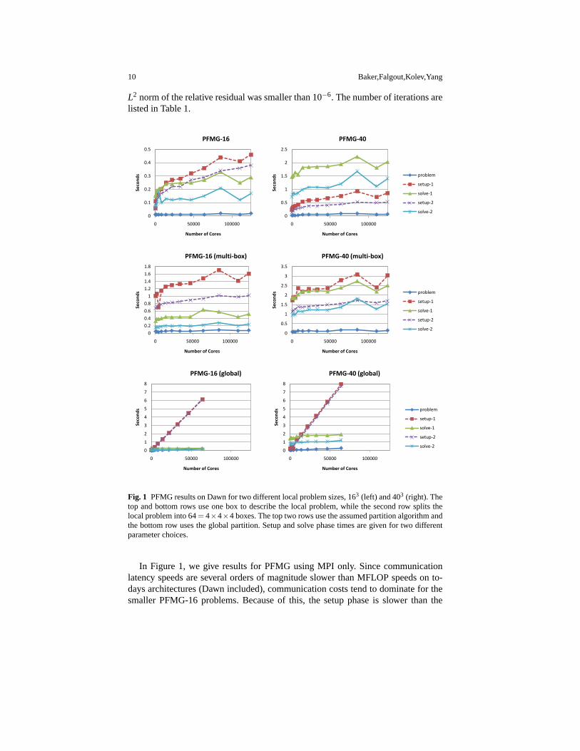
Fig. 1 PFMG results on Dawn for two different local problem sizes, 163 (left) and 403 (right). Thetop and bottom rows use one box to describe the local problem, while the second row splits thelocal problem into 64= 4×4×4 boxes. The top two rows use the assumed partition algorithm andthe bottom row uses the global partition. Setup and solve phase times are given for two differentparameter choices.

In Figure 1, we give results for PFMG using MPI only. Since communicationlatency speeds are several orders of magnitude slower than MFLOP speeds on to-days architectures (Dawn included), communication costs tend to dominate for thesmaller PFMG-16 problems. Because of this, the setup phase is slower than the

Scaling hypre’s solvers to 100,000 cores 11

solve phase, due primarily to the assumed partition and global partition compo-nents of the code. The global partition requiresO(PlogP) communications in thesetup phase, while the current implementation of the assumed partition requiresO((logP)2) communications (the latter is easier to see in Figure 2). It should bepossible to reduce the communication overhead of the assumed partition algorithmin the setup phase toO(logP) by implementing a feature for coarsening theboxmanagerin hypre (the box manager serves the role of thedistributed directoryin[4]). For PFMG-40 with the assumed partition, the setup phase is cheaper than thesolve phase for the single box case, and roughly the same cost for the multi-boxcase. For both multi-box cases, describing the data with 64 boxes leads to additionaloverhead in all phases, but the effect is more pronounced for the setup phase. Theproblem setup uses theStruct interface and is the least expensive component.

0

0.05

0.1

0.15

0.2

0.25

0.3

0.35

0.4

100 1000 10000 100000

Seco

nd

s

Number of Cores

PFMG-16-2

setup (smp)

solve (smp)

setup

solve

0

0.2

0.4

0.6

0.8

1

1.2

1.4

1.6

100 1000 10000

Seco

nd

s

Number of Cores

PFMG-16-2 (multi-box)

setup (smp)

solve (smp)

setup

solve

0

0.2

0.4

0.6

0.8

1

1.2

1.4

1.6

100 1000 10000 100000

Seco

nd

s

Number of Cores

PFMG-40-2

setup (smp)

solve (smp)

setup

solve

0

0.5

1

1.5

2

2.5

3

3.5

4

100 1000 10000 100000

Seco

nd

s

Number of Cores

PFMG-40-2 (multi-box)

setup (smp)

solve (smp)

setup

solve

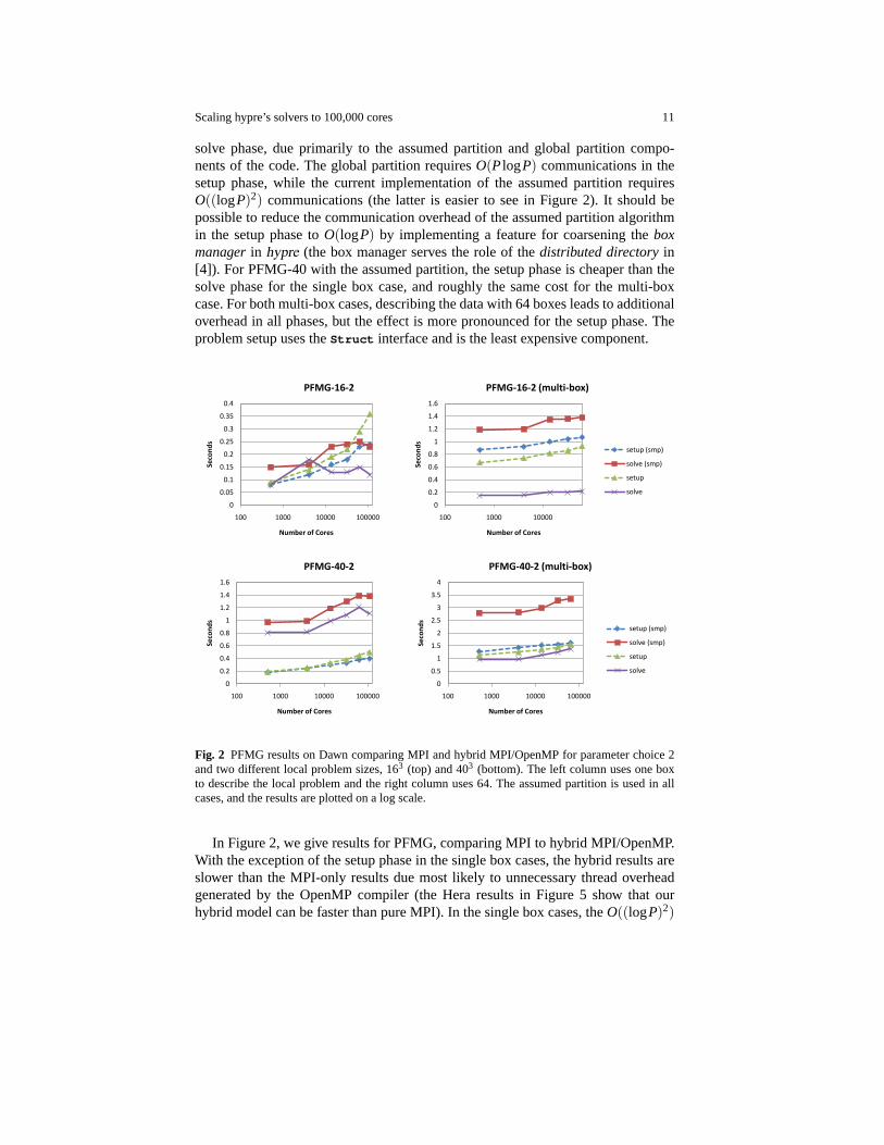
Fig. 2 PFMG results on Dawn comparing MPI and hybrid MPI/OpenMP for parameter choice 2and two different local problem sizes, 163 (top) and 403 (bottom). The left column uses one boxto describe the local problem and the right column uses 64. The assumed partition is used in allcases, and the results are plotted on a log scale.

In Figure 2, we give results for PFMG, comparing MPI to hybrid MPI/OpenMP.With the exception of the setup phase in the single box cases, the hybrid results areslower than the MPI-only results due most likely to unnecessary thread overheadgenerated by the OpenMP compiler (the Hera results in Figure 5 show that ourhybrid model can be faster than pure MPI). In the single box cases, theO((logP)2)

12 Baker,Falgout,Kolev,Yang

communications in the assumed partition algorithm dominates the time in the setupphase, so the pure MPI runs are slower than the hybrid runs due to the larger numberof boxes to manage. This scaling trend is especially apparent in the PFMG-16-2plot. For the multi-box cases, thread overhead is multiplied by a factor of 64 (eachthreaded loop becomes 64 threaded loops) and becomes the dominant cost.

The constant-coefficient CPFMG solver saves significantly on memory, but it wasonly slightly faster than the variable-coefficient PFMG case with nearly identicalscaling results. The memory savings allowed us to run CPFMG-200-2 to solve a1.049 trillion unknown problem on 131,072 cores (64× 64× 32) in 11 iterationsand 83.03 seconds. Problem setup took 0.84 seconds and solver setup took 1.10seconds.

0

5

10

15

20

25

30

35

40

45

50

0 50000 100000

Seco

nd

s

Number of Cores

SMG-40

problem

setup

solve

0

0.2

0.4

0.6

0.8

1

1.2

1.4

0 50000 100000

Seco

nd

s

Number of Processors

SysPFMG

problem

setup

solve

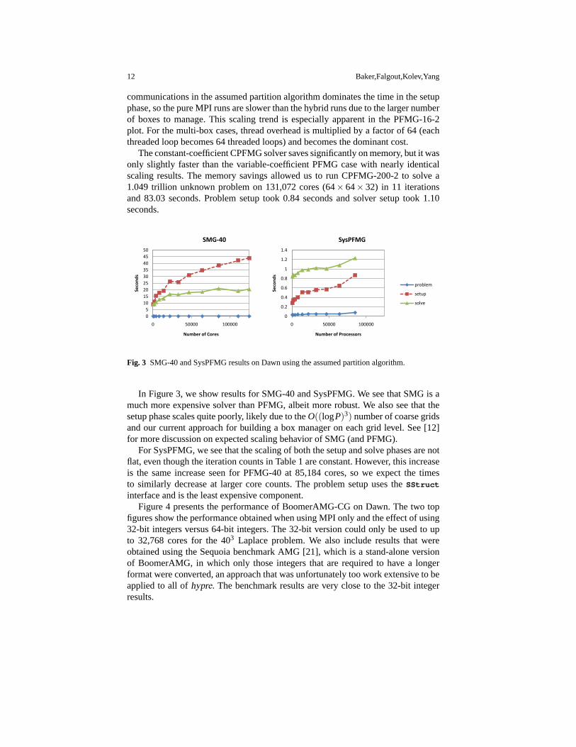
Fig. 3 SMG-40 and SysPFMG results on Dawn using the assumed partition algorithm.

In Figure 3, we show results for SMG-40 and SysPFMG. We see that SMG is amuch more expensive solver than PFMG, albeit more robust. We also see that thesetup phase scales quite poorly, likely due to theO((logP)3) number of coarse gridsand our current approach for building a box manager on each grid level. See [12]for more discussion on expected scaling behavior of SMG (and PFMG).

For SysPFMG, we see that the scaling of both the setup and solve phases are notflat, even though the iteration counts in Table 1 are constant. However, this increaseis the same increase seen for PFMG-40 at 85,184 cores, so we expect the timesto similarly decrease at larger core counts. The problem setup uses theSStruct

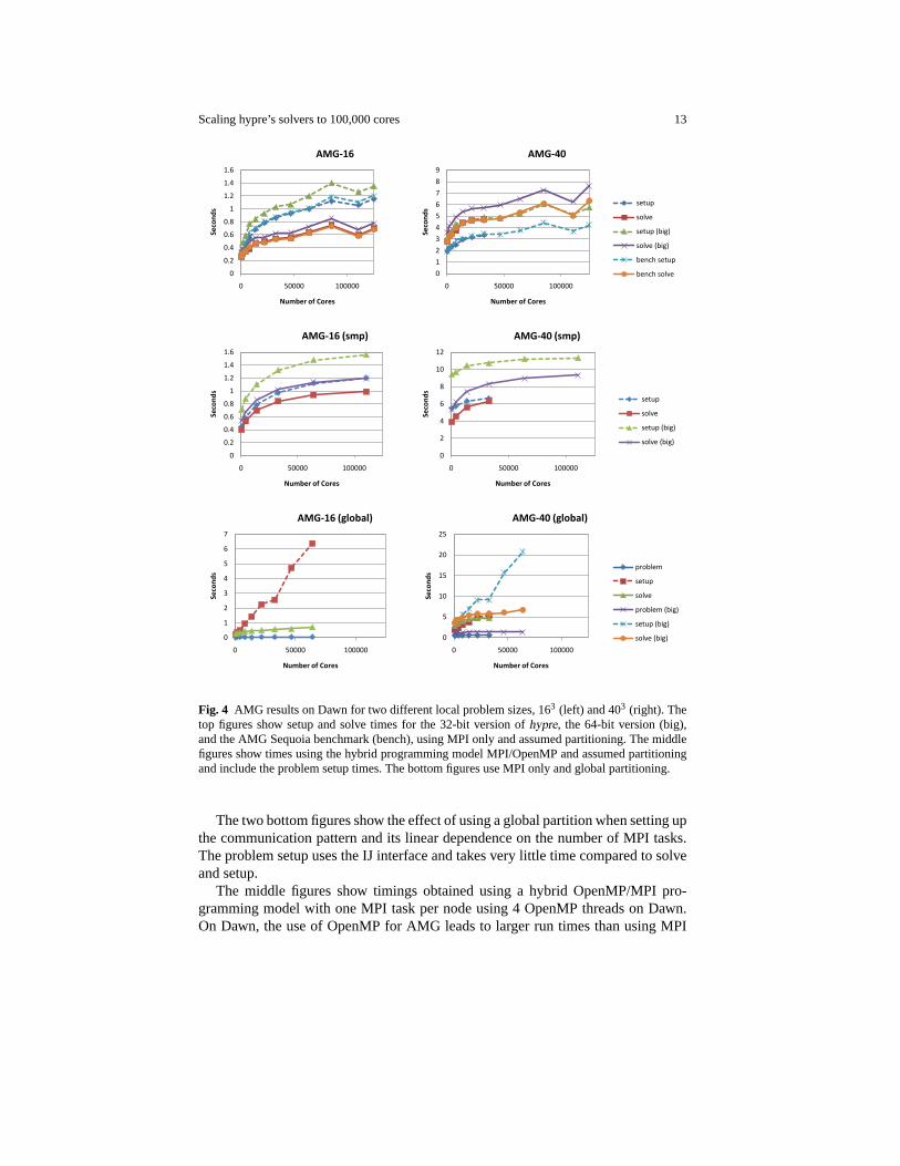
interface and is the least expensive component.Figure 4 presents the performance of BoomerAMG-CG on Dawn. The two top

figures show the performance obtained when using MPI only and the effect of using32-bit integers versus 64-bit integers. The 32-bit version could only be used to upto 32,768 cores for the 403 Laplace problem. We also include results that wereobtained using the Sequoia benchmark AMG [21], which is a stand-alone versionof BoomerAMG, in which only those integers that are required to have a longerformat were converted, an approach that was unfortunately too work extensive to beapplied to all ofhypre. The benchmark results are very close to the 32-bit integerresults.

Scaling hypre’s solvers to 100,000 cores 13

0

0.2

0.4

0.6

0.8

1

1.2

1.4

1.6

0 50000 100000

Seco

nd

s

Number of Cores

AMG-16

setup

solve

setup (big)

solve (big)

bench setup

bench solve 0

1

2

3

4

5

6

7

8

9

0 50000 100000

Seco

nd

s

Number of Cores

AMG-40

setup

solve

setup (big)

solve (big)

bench setup

bench solve

0

0.2

0.4

0.6

0.8

1

1.2

1.4

1.6

0 50000 100000

Seco

nd

s

Number of Cores

AMG-16 (smp)

setup

solve

setup (big)

solve (big)

0

2

4

6

8

10

12

0 50000 100000

Seco

nd

s

Number of Cores

AMG-40 (smp)

setup

solve

setup (big)

solve (big)

0

1

2

3

4

5

6

7

0 50000 100000

Seco

nd

s

Number of Cores

AMG-16 (global)

problem

setup

solve

0

5

10

15

20

25

0 50000 100000

Seco

nd

s

Number of Cores

AMG-40 (global)

problem

setup

solve

problem (big)

setup (big)

solve (big)

Fig. 4 AMG results on Dawn for two different local problem sizes, 163 (left) and 403 (right). Thetop figures show setup and solve times for the 32-bit version ofhypre, the 64-bit version (big),and the AMG Sequoia benchmark (bench), using MPI only and assumed partitioning. The middlefigures show times using the hybrid programming model MPI/OpenMP and assumed partitioningand include the problem setup times. The bottom figures use MPI only and global partitioning.

The two bottom figures show the effect of using a global partition when setting upthe communication pattern and its linear dependence on the number of MPI tasks.The problem setup uses the IJ interface and takes very little time compared to solveand setup.

The middle figures show timings obtained using a hybrid OpenMP/MPI pro-gramming model with one MPI task per node using 4 OpenMP threads on Dawn.On Dawn, the use of OpenMP for AMG leads to larger run times than using MPI

14 Baker,Falgout,Kolev,Yang

only and is therefore not recommended. While the solve phase of BoomerAMGis completely threaded, portions of it, like the multiplication of the transpose ofthe interpolation operator with a vector cannot be implemented as efficiently usingOpenMP as MPI with our current data structure. Also, portions of the setup phase,like the coarsening and part of the interpolation, are currently not threaded, whichalso negatively affects the performance when using OpenMP.

0

0.5

1

1.5

2

2.5

3

3.5

0 1000 2000 3000 4000

Seco

nd

s

Number of Cores

PFMG-16-1 on Hera

setup (16x1)

solve (16x1)

setup (4x4)

solve (4x4)

setup (1x16)

solve (1x16)0

0.5

1

1.5

2

2.5

3

3.5

4

0 1000 2000 3000 4000Se

con

ds

Number of Cores

PFMG-40-1 on Hera

setup (16x1)

solve (16x1)

setup (4x4)

solve (4x4)

setup (1x16)

solve (1x16)

0

1

2

3

4

5

6

7

8

9

0 1000 2000 3000 4000

Seco

nd

s

Number of Cores

AMG-16 on Hera

setup (16x1)

solve (16x1)

setup (4x4)

solve (4x4)

setup (1x16)

solve (1x16)0

2

4

6

8

10

12

14

16

18

0 1000 2000 3000 4000

Seco

nd

s

Number of Cores

AMG-40 on Hera

setup (16x1)

solve (16x1)

setup (4x4)

solve (4x4)

setup (1x16)

solve (1x16)

Fig. 5 Setup and solve times on Hera for PFMG and AMG, using an MPI only programming model(16x1), and two hybrid MPI/OpenMP programming models using 4 MPI tasks with 4 OpenMPthreads each (4x4) and using 1 MPI task with 16 OpenMP threads (1x16) per node.

On Hera, the use of a hybrid MPI/OpenMP versus an MPI only programmingmodel yields different results, see Figure 5. Since at most 4096 cores were availableto us, we used the global partition. We compare the MPI only implementations with16 MPI tasks per node (16x1) to a hybrid model using 4 MPI tasks with 4 OpenMPthreads each (4x4), which is best adapted to the architecture, and a hybrid modelusing 1 MPI task with 16 OpenMP threads per node (1x16). For the smaller problemwith 163 unknowns per core, we obtain the worst times using MPI only, followedby the 4x4 hybrid model. The best times are achieved using the 1x16 hybrid model,which requires the least amount of communication, since communication is veryexpensive compared to computation on Hera and communication dominates overcomputation for smaller problem sizes. The picture changes for the larger problemwith 403 unknowns per core. Now the overall best times are achieved using the 4x4

Scaling hypre’s solvers to 100,000 cores 15

hybrid model, which has less communication overhead than the MPI only model,but is not plagued by NUMA effects like the 1x16 hybrid model, where all memoryis located in the first memory module, causing large access times and contention forthe remaining 12 cores, see also [6].

0

1

2

3

4

5

6

7

8

9

10

0 50000 100000

Seco

nd

s

Number of Cores

AMS-16

problem

setup

solve

0

20

40

60

80

100

120

140

0 50000 100000

Seco

nd

s

Number of Cores

AMS-32 (big)

problem

setup

solve

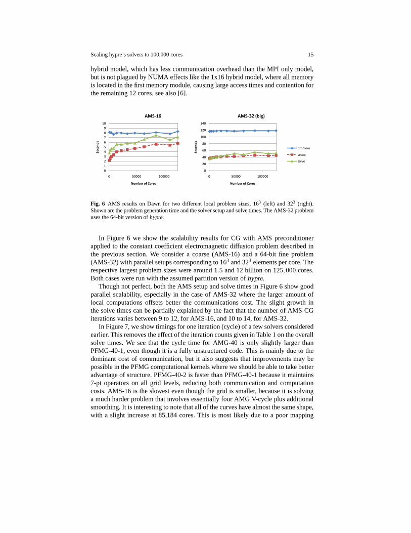
Fig. 6 AMS results on Dawn for two different local problem sizes, 163 (left) and 323 (right).Shown are the problem generation time and the solver setup and solve times. The AMS-32 problemuses the 64-bit version ofhypre.

In Figure 6 we show the scalability results for CG with AMS preconditionerapplied to the constant coefficient electromagnetic diffusion problem described inthe previous section. We consider a coarse (AMS-16) and a 64-bit fine problem(AMS-32) with parallel setups corresponding to 163 and 323 elements per core. Therespective largest problem sizes were around 1.5 and 12 billion on 125,000 cores.Both cases were run with the assumed partition version ofhypre.

Though not perfect, both the AMS setup and solve times in Figure 6 show goodparallel scalability, especially in the case of AMS-32 where the larger amount oflocal computations offsets better the communications cost. The slight growth inthe solve times can be partially explained by the fact that the number of AMS-CGiterations varies between 9 to 12, for AMS-16, and 10 to 14, for AMS-32.

In Figure 7, we show timings for one iteration (cycle) of a few solvers consideredearlier. This removes the effect of the iteration counts given in Table 1 on the overallsolve times. We see that the cycle time for AMG-40 is only slightly larger thanPFMG-40-1, even though it is a fully unstructured code. This is mainly due to thedominant cost of communication, but it also suggests that improvements may bepossible in the PFMG computational kernels where we should be able to take betteradvantage of structure. PFMG-40-2 is faster than PFMG-40-1 because it maintains7-pt operators on all grid levels, reducing both communication and computationcosts. AMS-16 is the slowest even though the grid is smaller, because it is solvinga much harder problem that involves essentially four AMG V-cycle plus additionalsmoothing. It is interesting to note that all of the curves have almost the same shape,with a slight increase at 85,184 cores. This is most likely due to a poor mapping

16 Baker,Falgout,Kolev,Yang

0.0000

0.1000

0.2000

0.3000

0.4000

0.5000

0.6000

0.7000

0 50000 100000

Seco

nd

s

Number of Cores

Cycle Times

PFMG-40-1

PFMG-40-2

AMG-40 (big)

AMS-16

Fig. 7 Cycle times on Dawn for CG with various multigrid preconditioners.

of the problem data to the hardware, which resulted in more costly long-distancecommunication.

We now comment on the performance improvements that can be achieved whenusing the struct interface and PFMG or CPFMG over the IJ interface and Boomer-AMG for suitable structured problems. For the smaller Laplace problem, PFMG-16-1 is about 2.5 times faster than the 32-version of AMG-16 and the AMG benchmark,and 3 times faster than the 64-bit version. The non-Galerkin version, PFMG-16-2,is about 3 to 4 times faster than AMG. For the larger problem, PFMG-40-2 is about7 times faster than the 64-bit version of AMG and about 5 times faster than thebenchmark.

Finally, we comment on the times it takes to set up the problems viahypre’sinterfaces. Figures 1, 3, and 4 showed that for many problems, the setup takes verylittle time compared to setup and solve times of the solvers. Note that the times forthe problem setup via the IJ interface in Figure 4 includes setting up the problemdirectly in the ParCSR data structure and then using the information to set up thematrix using the IJ data interface. Using the IJ interface directly for the problemsetup takes only about half as much time.

The problem generation time in Figure 6 corresponds to the assembly of theedge element Maxwell stiffness matrix and load vector, as well as the computationof the rectangular discrete gradient matrix and the nodal vertex coordinates neededfor AMS. These are all done with theSStruct interface, using its finite elementfunctionality for the stiffness matrix and load vector. Overall, the problem genera-tion time scales very well. Though its magnitude may appear somewhat large, oneshould account that it also includes the (redundant) computation of all local stiffnessmatrices, and the penalty from the use of the 64-bit version ofhypre in AMS-32.

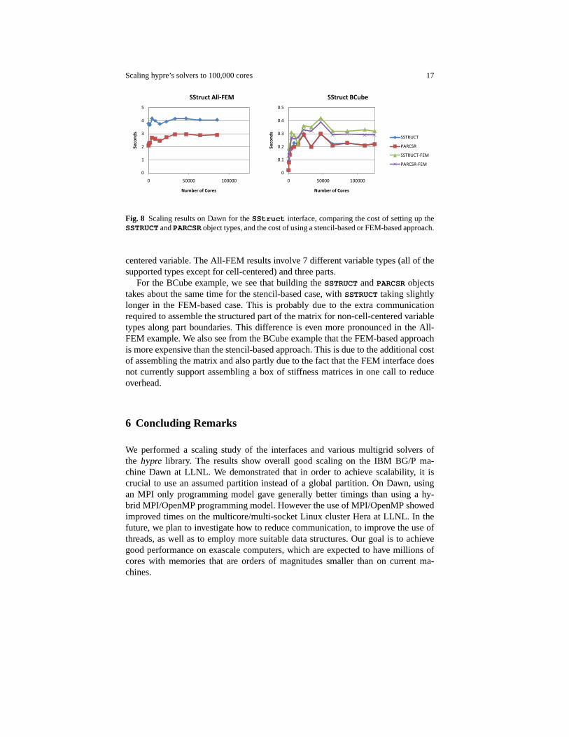
In Figure 8, we give results for theSStruct interface. The BCube stencil-based results involve one cell-centered variable and two parts connected by theGridSetNeighborPart() routine, while the BCube FEM-based results use a node-

Scaling hypre’s solvers to 100,000 cores 17

0

1

2

3

4

5

0 50000 100000

Seco

nd

s

Number of Cores

SStruct All-FEM

SSTRUCT

PARCSR

0

0.1

0.2

0.3

0.4

0.5

0 50000 100000

Seco

nd

s

Number of Cores

SStruct BCube

SSTRUCT

PARCSR

SSTRUCT-FEM

PARCSR-FEM

Fig. 8 Scaling results on Dawn for theSStruct interface, comparing the cost of setting up theSSTRUCTandPARCSRobject types, and the cost of using a stencil-based or FEM-based approach.

centered variable. The All-FEM results involve 7 different variable types (all of thesupported types except for cell-centered) and three parts.

For the BCube example, we see that building theSSTRUCTandPARCSRobjectstakes about the same time for the stencil-based case, withSSTRUCTtaking slightlylonger in the FEM-based case. This is probably due to the extra communicationrequired to assemble the structured part of the matrix for non-cell-centered variabletypes along part boundaries. This difference is even more pronounced in the All-FEM example. We also see from the BCube example that the FEM-based approachis more expensive than the stencil-based approach. This is due to the additional costof assembling the matrix and also partly due to the fact that the FEM interface doesnot currently support assembling a box of stiffness matrices in one call to reduceoverhead.

6 Concluding Remarks

We performed a scaling study of the interfaces and various multigrid solvers ofthe hypre library. The results show overall good scaling on the IBM BG/P ma-chine Dawn at LLNL. We demonstrated that in order to achieve scalability, it iscrucial to use an assumed partition instead of a global partition. On Dawn, usingan MPI only programming model gave generally better timings than using a hy-brid MPI/OpenMP programming model. However the use of MPI/OpenMP showedimproved times on the multicore/multi-socket Linux cluster Hera at LLNL. In thefuture, we plan to investigate how to reduce communication, to improve the use ofthreads, as well as to employ more suitable data structures. Our goal is to achievegood performance on exascale computers, which are expected to have millions ofcores with memories that are orders of magnitudes smaller than on current ma-chines.

18 Baker,Falgout,Kolev,Yang

PFMG- CPFMG-P 16-1 16-2 40-1 40-216-1 16-2 40-1 40-2SMG-40SysPFMG

64 9 9 10 10 9 9 9 9 5 9512 9 10 10 11 9 9 10 10 5 91728 10 10 10 11 9 9 10 10 5 94096 10 10 10 11 10 9 10 10 5 98000 10 11 10 11 10 10 10 10 6 913824 10 11 11 11 10 10 10 10 6 921952 10 11 11 12 10 10 10 11 6 932768 10 11 11 12 10 10 10 10 6 946656 10 11 11 12 10 10 10 11 6 964000 10 11 11 12 10 10 10 10 6 985184 10 11 11 13 10 10 10 10 6 9110592 10 11 11 13 10 10 10 11 6125000 10 11 11 13 10 10 10 12 6

AMG- AMS-P 16 16 (smp) 40 40 (smp)16 32

64 12 13512 14 14 15 16 9 101728 15 17 10 104096 15 15 18 18 10 118000 16 19 11 1113824 17 16 21 20 11 1121952 17 22 11 1232768 18 17 22 22 11 1346656 18 23 11 1464000 19 18 24 23 12 1385184 19 24 12 14110592 19 19 24 24 12 14125000 19 27 12 14

AMG-16 AMG-40P (16x1) (4x4) (1x16)(16x1) (4x4) (1x16)

64 12 12 12 13 13 14512 14 13 14 15 16 161728 15 14 14 17 17 184096 15 15 15 18 19 20

Table 1 Iteration counts on Dawn (top two tables) and Hera (bottom table). For all solvers, itera-tions were stopped when the relative residual was smaller than 10−6.

References

1. S. F. Ashby and R. D. Falgout. A parallel multigrid preconditioned conjugate gradient algo-rithm for groundwater flow simulations.Nuclear Science and Engineering, 124(1):145–159,September 1996. UCRL-JC-122359.

2. A. Baker, R. Falgout, T. Gamblin, T. Kolev, M. Schulz, and U. M. Yang. Scaling algebraicmultigrid solvers: On the road to exascale. InProceedings of Competence in High Perfor-mance Computing (CiHPC 2010), 2011. To appear. Also available as LLNL Tech. Report

Scaling hypre’s solvers to 100,000 cores 19

LLNL-PROC-463941.3. A. H. Baker, R. D. Falgout, T. V. Kolev, and U. M. Yang. Multigrid smoothers for ultra-parallel

computing. 2010. (submitted). Also available as a Lawrence Livermore National Laboratorytechnical report LLNL-JRNL-435315.

4. A. H. Baker, R. D. Falgout, and U. M. Yang. An assumed partition algorithm for determiningprocessor inter-communication.Parallel Computing, 32(5–6):394–414, 2006. UCRL-JRNL-215757.

5. A. H. Baker, T. Gamblin, M. Schulz, and U. M. Yang. Challenges of scaling algebraic multi-grid across modern multicore architectures. InProceedings of the 25th IEEE InternationalParallel and Distributed Processing Symposium (IPDPS 2011), 2011. LLNL-CONF-458074.

6. A. H. Baker, M. Schulz, and U. M. Yang. On the performance of an algebraic multi-grid solver on multicore clusters. In J.M.L.M. Palma et al., editor,VECPAR 2010, vol-ume 6449 ofLecture Notes in Computer Science, pages 102–115. Springer-Verlag, 2011.http://vecpar.fe.up.pt/2010/papers/24.php.

7. C. Baldwin, P. N. Brown, R. D. Falgout, J. Jones, and F. Graziani. Iterative linear solvers ina 2d radiation-hydrodynamics code: methods and performance.J. Comput. Phys., 154:1–40,1999. UCRL-JC-130933.

8. A. Brandt, S. F. McCormick, and J. W. Ruge. Algebraic multigrid (AMG) for sparse matrixequations. In D. J. Evans, editor,Sparsity and Its Applications. Cambridge University Press,Cambridge, 1984.

9. P. N. Brown, R. D. Falgout, and J. E. Jones. Semicoarsening multigrid on distributed memorymachines.SIAM J. Sci. Comput., 21(5):1823–1834, 2000. Special issue on the Fifth CopperMountain Conference on Iterative Methods. UCRL-JC-130720.

10. R. Falgout, J. Jones, and U. M. Yang. Pursuing scalability for hypre’s conceptual interfaces.ACM ToMS, 31:326–350, 2005.

11. R. D. Falgout. An introduction to algebraic multigrid.Computing in Science and Engineering,8(6):24–33, 2006. Special issue on Multigrid Computing. UCRL-JRNL-220851.

12. R. D. Falgout and J. E. Jones. Multigrid on massively parallel architectures. In E. Dick,K. Riemslagh, and J. Vierendeels, editors,Multigrid Methods VI, volume 14 ofLecture Notesin Computational Science and Engineering, pages 101–107. Springer-Verlag, 2000. Proc.of the Sixth European Multigrid Conference held in Gent, Belgium, September 27-30, 1999.UCRL-JC-133948.

13. H. Gahvari, A. H. Baker, M. Schulz, U. M. Yang, K. E. Jordan, and W. Gropp. Modeling theperformance of an algebraic multigrid cycle on HPC platforms. InProceedings of the 25thInternational Conference on Supercomputing (ICS 2011), 2011. To appear. Also available asLLNL Tech. Report LLNL-CONF-473462.

14. V. Henson and U. Yang. BoomerAMG: A parallel algebraic multigrid solver and precondi-tioner. Appl. Numer. Math., 41:155–177, 2002.

15. hypre: High performance preconditioners. http://www.llnl.gov/CASC/hypre/.16. T. Kolev and P. Vassilevski. Parallel auxiliary space AMG for H(curl) problems.J. Com-

put. Math., 27:604–623, 2009. Special issue on Adaptive and Multilevel Methods in Elec-tromagnetics. Also available as a Lawrence Livermore National Laboratory technical reportUCRL-JRNL-237306.

17. U. Meier and A. Sameh. The behavior of conjugate gradient algorithms on a multivectorprocessor with a hierarchical memory.J. Comp. Appl. Math., 24:13–32, 1988.

18. J. W. Ruge and K. Stuben. Algebraic multigrid (AMG). In S. F. McCormick, editor,MultigridMethods, volume 3 ofFrontiers in Applied Mathematics, pages 73–130. SIAM, Philadelphia,PA, 1987.

19. Y. Saad. Iterative Methods for Sparse Linear Systems. Society for Industrial and AppliedMathematics, 2nd edition, 2003.

20. S. Schaffer. A semi-coarsening multigrid method for elliptic partial differential equationswith highly discontinuous and anisotropic coefficients.SIAM J. Sci. Comput., 20(1):228–242,1998.

21. Sequoia. ASC sequoia benchmark codes. https://asc.llnl.gov/sequoia/benchmarks/.

20 Baker,Falgout,Kolev,Yang

22. H. D. Sterck, R. D. Falgout, J. W. Nolting, and U. M. Yang. Distance-two interpolation forparallel algebraic multigrid.Numer. Linear Algebra Appl., 15(2–3):115–139, 2008. Specialissue on Multigrid Methods. UCRL-JRNL-230844.

23. H. D. Sterck, U. M. Yang, and J. J. Heys. Reducing complexity in parallel algebraic multigridpreconditioners.SIAM J. Matrix Anal. Appl., 27(4):1019–1039, 2006.

24. K. Stuben. Algebraic multigrid (AMG): an introduction with applications. In U. Hackbusch,C. Oosterlee, and A. Schueller, editors,Multigrid. Academic Press, 2000.

25. U. Yang. Parallel algebraic multigrid methods - high performance preconditioners. In A. Bru-aset and A. Tveito, editors,Numerical Solution of Partial Differential Equations on ParallelComputers, volume 51, pages 209–236. Springer-Verlag, 2006.

26. U. M. Yang. On long range interpolation operators for aggressive coarsening.Numer. LinearAlgebra Appl., 17:453–472, 2010. LLNL-JRNL-417371.