Scale Recovery for Monocular Visual Odometry Using Depth...
9
Scale Recovery for Monocular Visual Odometry Using Depth Estimated with Deep Convolutional Neural Fields Xiaochuan Yin * , Xiangwei Wang * , Xiaoguo Du, Qijun Chen Tongji University [email protected],[email protected], {1610448, qjchen}@tongji.edu.cn Abstract Scale recovery is one of the central problems for monoc- ular visual odometry. Normally, road plane and camera height are specified as reference to recover the scale. The performances of these methods depend on the plane recog- nition and height measurement of camera. In this work, we propose a novel method to recover the scale by incor- porating the depths estimated from images using deep con- volutional neural fields. Our method considers the whole environmental structure as reference rather than a speci- fied plane. The accuracy of depth estimation contributes to the scale recovery. We improve the performance of depth estimation by considering two consecutive frames and ego- motion of camera into our networks. The depth refinement and scale recovery are obtained iteratively. In this way, our method can eliminate the scale drift and improve the depth estimation simultaneously. The effectiveness of our method is verified on the KITTI dataset for both monocular visual odometry and depth estimation tasks. 1. Introduction Visual odometry is the process of estimating the egomo- tion of the robot from input images. It is one of the core modules of simultaneous localization and mapping (SLAM) system. Visual odometry using stereo camera has achieved a great success these years. The reason why stereo visual odometry is widely applied is that it can estimate a reliable depth map for transformation matrix calculation. However, stereo camera will degenerate into a monocular one when the distance between camera and scene is much larger than the baseline. Moreover, self-calibration is also required for stereo visual odometry system after long-term operation in order to reduce the mechanical vibration encountered in ap- plication [5, 23]. Unlike the stereo visual odometry, vi- sual odometry using monocular camera does not suffer from these problems. Therefore, monocular visual odometry has * Authors contributed equally Figure 1. 3D reconstruction of street scene with egomotion and depth estimated by our method. attracted a lot of attentions in recent years. Monocular visual odometry algorithms cannot get en- vironment map and robot motion in real scale. Because the distance between features and camera cannot be mea- sured by triangulation directly. Therefore, monocular visual odometry faces the problem of scale drift, and the absolute scale need to be recovered to eliminate it. To recover the scale, geometry constraints between the camera and the surroundings are normally used. Previous methods apply the camera height and the ground surface to obtain the scale [2, 24, 15]. The camera height is assumed to be known in advance. In [2], they adopt a texture analy- sis classifier to extract the ground region, and in this way the planar homography matrix is calculated to recover the scale factor. In [24], a combination of several cues within a prede- fined region of interest (ROI) is used to recover the scale. To be more robust in different scenes, [15] estimates the ground geometry with self-learned ground appearance information. These methods are constrained by limited environmental in- formation. More structural information of environments is required. In this way, there would not need to set the camera height and ground plane as the fixed references. In these years, deep learning has achieved a great success 5870
Transcript of Scale Recovery for Monocular Visual Odometry Using Depth...

Scale Recovery for Monocular Visual Odometry Using Depth Estimated with
Deep Convolutional Neural Fields
Xiaochuan Yin∗, Xiangwei Wang∗, Xiaoguo Du, Qijun Chen
Tongji University
[email protected],[email protected], 1610448, [email protected]
Abstract
Scale recovery is one of the central problems for monoc-
ular visual odometry. Normally, road plane and camera
height are specified as reference to recover the scale. The
performances of these methods depend on the plane recog-
nition and height measurement of camera. In this work,
we propose a novel method to recover the scale by incor-
porating the depths estimated from images using deep con-
volutional neural fields. Our method considers the whole
environmental structure as reference rather than a speci-
fied plane. The accuracy of depth estimation contributes to
the scale recovery. We improve the performance of depth
estimation by considering two consecutive frames and ego-
motion of camera into our networks. The depth refinement
and scale recovery are obtained iteratively. In this way, our
method can eliminate the scale drift and improve the depth
estimation simultaneously. The effectiveness of our method
is verified on the KITTI dataset for both monocular visual
odometry and depth estimation tasks.
1. Introduction
Visual odometry is the process of estimating the egomo-
tion of the robot from input images. It is one of the core
modules of simultaneous localization and mapping (SLAM)
system. Visual odometry using stereo camera has achieved
a great success these years. The reason why stereo visual
odometry is widely applied is that it can estimate a reliable
depth map for transformation matrix calculation. However,
stereo camera will degenerate into a monocular one when
the distance between camera and scene is much larger than
the baseline. Moreover, self-calibration is also required for
stereo visual odometry system after long-term operation in
order to reduce the mechanical vibration encountered in ap-
plication [5, 23]. Unlike the stereo visual odometry, vi-
sual odometry using monocular camera does not suffer from
these problems. Therefore, monocular visual odometry has
∗Authors contributed equally
Figure 1. 3D reconstruction of street scene with egomotion and
depth estimated by our method.
attracted a lot of attentions in recent years.
Monocular visual odometry algorithms cannot get en-
vironment map and robot motion in real scale. Because
the distance between features and camera cannot be mea-
sured by triangulation directly. Therefore, monocular visual
odometry faces the problem of scale drift, and the absolute
scale need to be recovered to eliminate it.
To recover the scale, geometry constraints between the
camera and the surroundings are normally used. Previous
methods apply the camera height and the ground surface to
obtain the scale [2, 24, 15]. The camera height is assumed
to be known in advance. In [2], they adopt a texture analy-
sis classifier to extract the ground region, and in this way the
planar homography matrix is calculated to recover the scale
factor. In [24], a combination of several cues within a prede-
fined region of interest (ROI) is used to recover the scale. To
be more robust in different scenes, [15] estimates the ground
geometry with self-learned ground appearance information.
These methods are constrained by limited environmental in-
formation. More structural information of environments is
required. In this way, there would not need to set the camera
height and ground plane as the fixed references.
In these years, deep learning has achieved a great success
15870

in the computer vision field for its powerful feature learning
ability. Deep learning may promote the progress of visual
odometry [1]. In [4], estimator based on deep convolution
neural networks is trained for egomotion estimation from
optical flow. Depth estimation of surroundings would be an-
other plausible direction for this problem. Depth estimation
from single image is a challenging task. Depth estimation
and scene structure inference with Markov Random Field
(MRF) is proposed in [22]. In [6, 7], a novel pixel-wise
depth and surface normal regression neural networks are
proposed. Depth can also be refined via hierarchical condi-
tional random fields (CRFs) after regression from deep con-
volutional networks [17]. In [18], deep convolutional neu-
ral networks combined with condition random fields (con-
volutional neural fields) are applied to estimate depth from
picture taken in indoor and outdoor environments. For con-
secutive frames, optical flow is applied to extract depth in-
formation [12, 21].
In this paper, we introduce a novel scale recovery method
using depth estimated from images with deep neural net-
works. We calculate the scale of translation from the esti-
mated depth map. The depth prediction is improved by con-
sidering consecutive images and motion constraints into our
method. Therefore, convolutional neural fields are used for
depth estimation in our system, which concatenate convolu-
tional neural networks and conditional random fields. The
convolutional neural networks can regress a coarse depth
map from input images. Then the conditional random fields
refine the coarse depth by involving the constraints. The
scale of egomotion is obtained based on the refined depth.
In this way, the depth and scale can be calculated iteratively.
The contributions of our paper are as follows.
1. We present a novel scale recovery method for monoc-
ular visual odometry.
2. We present novel neural networks for depth estimation
from images. It takes consecutive frames and motion
constraints into consideration to improve the result.
3. Our method can alleviate the scale drift problem
caused by the accumulated error.
4. A novel monocular visual odometry system is pro-
posed using deep learning.
The structure of this paper is organized as follows. In
section II, we introduce the background knowledge of the
relationship between photo intensity and camera motion.
The neural networks for depth estimation with consecu-
tive pictures and egomotion are proposed in section III. In
section IV, we introduce our scale calculation method and
framework of our system. Experiments are conducted and
analyzed in section V. We conclude our paper in the last
section.
2. Background
In this section, we introduce the background knowledge
of our system. In this paper, bold capital letters denote a ma-
trix, bold lower-case letters a column vector, others a scalar.
The intensity of pixel u = (u, v)T ∈ Ω in the image is
I : Ω ⊂ R2 7→ R. The 3D point in the world coordinate
p = (x, y, z)T ∈ R3 of the pixel u can be obtained from
the inverse projection function π : R2 7→ R3.
p = π−1(u, zu) = zu
(
u− cx
fx,v − cy
fy, 1
)T
(1)
where zu is the depth of pixel u, fx, fy and cx, cy denotes
the focal length and optical center in the standard pinhole
camera model, respectively.
The rotation matrix R ∈ SO(3) and translation vector
t ∈ R3 can transform the point p to the new position.
T (T,p) = Rp+ t (2)
The residual of the i-th pixel is defined as the difference
in intensity between the first and second image. In this
work, the intensity of pixels after reprojection is assumed
to be the same.
ri,I := I2(
π(
T(
T, π−1 (u1,i, z1,ui))))
− I1(u1,i) (3)
R =
u|u ∈ Rk−1 ∧ π(
T(
T, π−1 (u, zu)))
∈ Ωk
(4)
where π is the projection function which is defined as:
u = π(p) =
(
fxx
z+ cx,
fyy
z+ cy
)
.
3. Depth Estimation with Convolutional Neu-
ral Fields
In this section, we will introduce the structure of our
deep neural networks for depth estimation. In order to in-
crease the accuracy of depth prediction and remove the out-
liers, two consecutive images and the egomotion are taken
as inputs in our networks. We construct our convolutional
neural fields by concatenating the convolutional neural net-
works and conditional random fields.
We apply the deep residual neural networks (ResNet)
[10] and fully convolutional networks [19] to construct the
convolutional part of our networks. ResNet is an elegant
structure, and it has achieved excellent performances [10].
It takes standard convolutional neural networks and adds
skip connections that bypass a few convolutional layers to
construct the residual block. ResNet has a powerful abil-
ity for feature representation. However, convolutional and
pooling layers would generate the downsampling features.
5871

For the scale recovery problem, we need the depth values of
whole image. We apply the fully convolutional networks to
upsampling the regressed depth map to the input’s size. In
order to refine the depth map for later use, we apply the con-
ditional random fields to smooth the regressed result. The
structure of our neural networks is shown in Figure 2. The
detail of this part can refer to their elegant work in [10] [19].
Next, we will present our conditional random fields part for
depth refinement.
3.1. Refining the regression results via CRFs
Depth can be predicted using convolutional part men-
tioned above. However, output of the above networks has
outliers and may introduce additional errors for the scale
recovery process. Therefore, additional layer is required to
refine the generated depth. Conditional random fields are
commonly used to involve constraints to improve the re-
sults. In this work, we define an energy function as follows.
E =∑
p∈Ω1
U(y1,p, x1,p) + ω1
∑
(p,q)∈Ω1
V (y1,p, y1,q, x1,p, x1,q)
+ω2
∑
(p,q)∈R
W (x1,p, y1,p, x2,q,T)
(5)
where xi,p denotes the pixel p in image Ωi. yi,p is the depth
of pixel p in image Ωi. T is the transformation matrix of
robot. ω1 and ω2 are coefficients of last two terms. They
reflect the influences of each part, and they are obtained in
our training process. Our energy function consists of three
potential functions: unary potential, pairwise potential in
the same image and pairwise potential of two consecutive
images.
3.1.1 Unary potential
The unary potential function measures the least square loss
between the regressed depth z and ground truth depth y.
The regressed depth z is the output of the convolutional part
and it is taken as input to the conditional random fields for
refinement. The unary potential part is defined as:
U(y1,p, x1,p; θ) =1
2(y1,p − z1,p(x1,p; θ))
2, ∀p ∈ Ω1
(6)
where θ are the parameters of the convolutional part of our
networks.
3.1.2 Pairwise potential in the same image
The pairwise potential term enforces the coherent of neigh-
boring pixel’s depth. We assume that the neighboring pixels
with similar color are close in depth.
V (yp, yq, xp, xq; γ1, γ2) =1
2Rpq(yp−yq)
2, ∀p,q ∈ Ω1
(7)
where Rp,q is the appearance kernel, which is used to mea-
sure the distance and color between different pixels.
Rp,q = exp(−γ1‖Ip − Iq‖2 − γ2‖up − uq‖
2) (8)
where Ip and up are the color and position of the pixel p;
γ1 and γ2 denote the importance of each kernel.
3.1.3 Pairwise potential of two consecutive images
In order to consider the constraints between two consecu-
tive images, the third potential function measures accuracy
of depth estimation by projecting the current frame to the
previous one with known transformation matrix. Because
the intensity error r does not follow the Gaussian distribu-
tion. Therefore, the Huber loss function is applied in our
energy function to eliminate the effects of outliers.
W =1
2‖ri(T,u, z) + Ji(y − z)‖Huber (9)
where Ji is the Jacobian of the ri at pixel u with depth point
z and transformation matrix T.
3.2. Training the neural networks
The probability distribution function of depth is
Pr(y|x) =1
Z(x)exp(−E(y,x)) (10)
The partition function Z(x) is defined as:
Z(x1,x2,T) =
∫
y
exp−E(y,x1,x2,T)dy. (11)
Because the Huber loss function is applied in our energy
function, we cannot obtain the partition function for max-
imum a posteriori estimation by calculating the integral in
the partition function analytically. Therefore, the neural net-
works are trained through the score matching [11] without
requiring normalization. The discrete version of the score
matching is adopted to optimize the objective function
J (δ) =1
N
N∑
i=1
∑
δ
(
∂ϕi(δ) +1
2ϕi(δ)
2
)
+ const (12)
where δ = [z(θ)T, ω1, ω2]
T are the parameters to optimize
in conditional random fields. The score function is defined
as:
ϕ(y; δ) = ∇y logPr(y|δ) (13)
5872

ResNet+FCN CRFs
Frame 1
Frame 2
Depth Regression Depth Refining
Transformation Matrix
Figure 2. Structure of our neural networks. The inputs of neural networks are two consecutive frames and transformation matrix. Output is
the refined depth map. The deep convolutional part is composed of deep residual networks and fully convolutional networks. The output
of the convolutional part is refined by the following conditional random fields layer.
The i-th element of the model score function with respect
to the i-th variable is
∂iϕi(y; δ) =∂ϕi(y; δ)
∂yi(14)
The variable δ can be optimized with gradient descent
δ ← δ − η∂J
∂δ. (15)
The parameters of our convolutional neural fields
θ, ω1, ω2 can be obtained by backpropagation.
3.3. Depth estimation
The refined depth can be calculated by solving the MAP
inference
y = argmaxy
logPr(y|x1,x2,T). (16)
In the depth estimation process, the Huber loss function is
replaced with mean squared loss if the intensity error of pix-
els in two consecutive frames is smaller than a given thresh-
old, otherwise the depth value is removed.
The negative log-likelihood can be written as:
− logPr(y|x1,x2,T) =
1
N
(
‖y − z‖2 + ω1yTMy + ω2‖r+ J(y − z)‖2
)
(17)
where N is the number of inliers; M = D−R is the graph
Laplacian matrix; R is the affinity matrix composed of Rpq;
D is the diagonal matrix with Dpp =∑
q Rpq; J is the
Jacobian matrix of the image with respect of the depth, and
J is the diagonal matrix with Jpp = Jp.
The refined depth can be calculated as:
y =(
I+ ω1M+ ω2J2)−1 (
z+ ω2J2z− ω2Jr
)
(18)
The training process of our neural networks is shown
in Algorithm 1. We train the neural networks with mean
squared loss as criteria at first. Then the CRFs layer is added
and we train the whole networks. The errors and gradients
are set to zeros for the pixel without ground truth depth.
Algorithm 1: Training process of convolutional neural
fields
Input: Given the input image sequence XiNi=1,
Xi ∈ R3×m×n, the corresponding output
depth maps YiNi=1, Yi ∈ R
m×n and the
transformation matrix TiNi=1
Initialize: ResNet is obtained from model zoo.
Output: Parameters of networks θ, ω1 and ω2
// Pre-training the ResNet+FCN with mean squared
loss
// Training the networks include the CRFs layer
for t = 1 to maxIteration do
Randomly select input Xti, X
t+1i and T
// Forward propagation
Obtain refined depth map Yi
Obtain the gradient from Eq. (15)
//Backpropagation
Update θ, ω1 and ω2
end
return θ, ω1 and ω2
4. Scale Recovery with Estimated Depth
The initial egomotion Tt−1t can be obtained by minimiz-
ing the reprojection error from matched ORB features[20].
5873
However, the obtained egomotion is not in real scale. This
will cause the scale drift for the monocular visual odome-
try system. In this section, we introduce our scale recovery
method using depth map predicted from section 3.
The observed point position relative to current camera
coordinates is denoted by p = (xci , y
ci , z
ci )
T∈ R
3. The
scale parameter α can be obtained by solving
zc′i
ui
vi1
= α
fx 0 cx0 fy cy0 0 1
xci
ycizci
∀i = 1, 2, . . . , n
(19)
where zc′i is the estimated depth value in pixel ui(ui, vi).We denote Z (ui, vi) = zc′i . The estimated depth value for
each point can be express as:
zc′i = Z
(
xci
zcifx + cx,
ycizci
fy + cy
)
(20)
and the scale parameter is defined as:
α =zc′izci
(21)
Therefore, the residual of the i-th observed map point can
be written as:
ri = zc′i − αzci . (22)
Ideally, the residual would be zero. On account of the
noise introduced by the estimated depth and the noise is
independent and identically distributed (IID), the distribu-
tion of ri denotes p(ri). Because we use the matched fea-
ture points to calculate the scale. The number of points
left is small. Taking small sample size and existence of
outliers into consideration, the non-standardized student’s
t-distribution is adopted to model this distribution, which is
capable of modeling the data with outliers. Then the scale
recovery problem can be represented as a maximum likeli-
hood estimation:
α = argmaxα
n∏
i
p(ri) (23)
where
p(ri) ∝1
σ
(
1 +1
υ
(ri
σ
)2)− υ+1
2
(24)
where σ and υ are the scaling parameter and degree of free-
dom of student’s t-distribution; α is the scale parameter to
recover.
The maximum likelihood estimation can be solved by
expectation maximization (EM) algorithm via calculating
α and σ [13, 14] iteratively. Then we can obtain the trans-
formation matrix with the scale α as
Tt−1t =
(
Rt−1t αtt−1
t
0 1
)
(25)
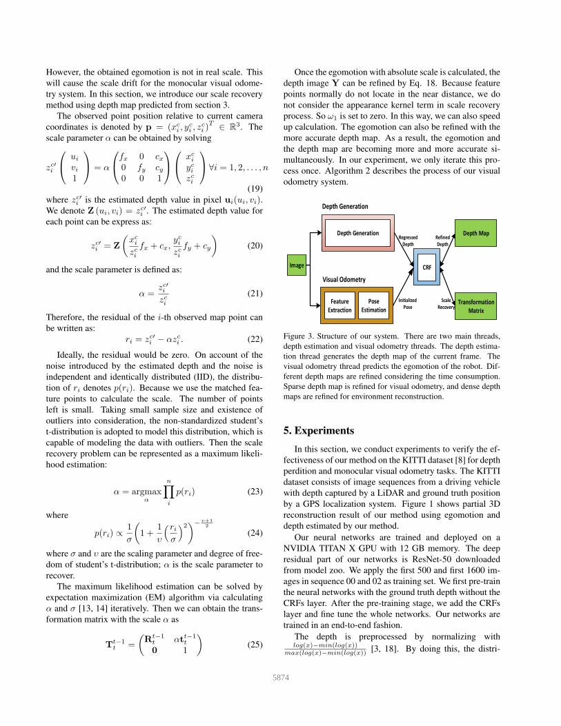
Once the egomotion with absolute scale is calculated, the
depth image Y can be refined by Eq. 18. Because feature
points normally do not locate in the near distance, we do
not consider the appearance kernel term in scale recovery
process. So ω1 is set to zero. In this way, we can also speed
up calculation. The egomotion can also be refined with the
more accurate depth map. As a result, the egomotion and
the depth map are becoming more and more accurate si-
multaneously. In our experiment, we only iterate this pro-
cess once. Algorithm 2 describes the process of our visual
odometry system.
Image
Feature
Extraction
Pose
Estimation
Visual Odometry
Depth Generation
Depth MapDepth Generation
Transformation
Matrix
CRF
Regressed
Depth
Initialized
Pose
Scale
Recovery
Refined
Depth
Figure 3. Structure of our system. There are two main threads,
depth estimation and visual odometry threads. The depth estima-
tion thread generates the depth map of the current frame. The
visual odometry thread predicts the egomotion of the robot. Dif-
ferent depth maps are refined considering the time consumption.
Sparse depth map is refined for visual odometry, and dense depth
maps are refined for environment reconstruction.
5. Experiments
In this section, we conduct experiments to verify the ef-
fectiveness of our method on the KITTI dataset [8] for depth
perdition and monocular visual odometry tasks. The KITTI
dataset consists of image sequences from a driving vehicle
with depth captured by a LiDAR and ground truth position
by a GPS localization system. Figure 1 shows partial 3D
reconstruction result of our method using egomotion and
depth estimated by our method.
Our neural networks are trained and deployed on a
NVIDIA TITAN X GPU with 12 GB memory. The deep
residual part of our networks is ResNet-50 downloaded
from model zoo. We apply the first 500 and first 1600 im-
ages in sequence 00 and 02 as training set. We first pre-train
the neural networks with the ground truth depth without the
CRFs layer. After the pre-training stage, we add the CRFs
layer and fine tune the whole networks. Our networks are
trained in an end-to-end fashion.
The depth is preprocessed by normalizing withlog(x)−min(log(x))
max(log(x)−min(log(x)) [3, 18]. By doing this, the distri-
5874
Algorithm 2: Scale recovery using depth predicted
from image
Input: Given the image sequence Xtnt=1,
corresponding regressed depth images
Ztnt=1 and camera parameters.
Initialize: α = 1, T1 is the camera pose relative to the
robot coordinate.
Output: The camera poses Ttnt=1 and the
optimized sparse depth images Ytnt=1
for t = 2 to n do// Calculate the transformation matrix
Extract and match feature points
Minimize the reprojection error to calculate
transformation matrix Tt−1t =
(
Rt−1t tt−1
t
0 1
)
// Scale parameter calculation
Obtain k map points piki=1,pi ∈ R
3
while i < maxIteration doCalculate the corresponding depth
zc′i ki=1, z
c′i ∈ R
Get the scale parameter α using maximum
likelihood estimation from Eq. (23)
Update Tt−1t =
(
Rt−1t αtt−1
t
0 1
)
Optimize the depth image Yt from Eq. (18)
end
Set Yt = Yt
Get current pose Tt = Tt−1t Tt−1
end
return Ttnt=1,Yt
nt=1
bution of depth is similar to a Gaussian distribution.
Unlike the depth prediction methods proposed in [17,
18], we do not apply super pixels in our framework. ORB
features are applied in our method. Because ORB features
are sparse in images, potential function in the same image is
not involved in our depth refining process in visual odom-
etry thread. This can accelerate the calculation of our pro-
gram.
Figure 3 shows that the structure of our system contains
two threads: depth generation thread and visual odome-
try thread. The depth generation thread provides regressed
depth values to visual odometry thread. Egomotion ob-
tained from visual odometry thread is passed to depth gen-
eration thread to get the refined depth. In order to accel-
erate the depth refining process in visual odometry subsys-
tem, only depths of sparse feature points are refined. After
obtaining the robot motion, the dense depth map can be ob-
tained later or in a different thread.
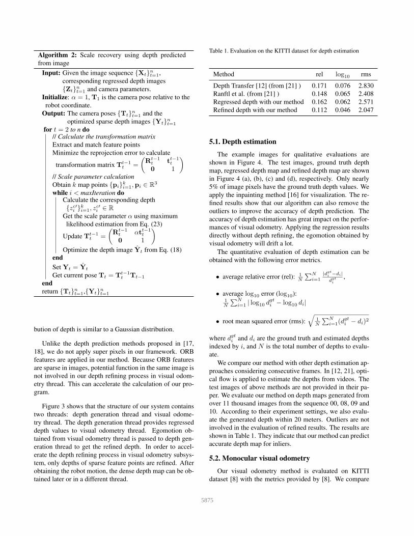
Table 1. Evaluation on the KITTI dataset for depth estimation
Method rel log10 rms
Depth Transfer [12] (from [21] ) 0.171 0.076 2.830
Ranftl et al. (from [21] ) 0.148 0.065 2.408
Regressed depth with our method 0.162 0.062 2.571
Refined depth with our method 0.112 0.046 2.047
5.1. Depth estimation
The example images for qualitative evaluations are
shown in Figure 4. The test images, ground truth depth
map, regressed depth map and refined depth map are shown
in Figure 4 (a), (b), (c) and (d), respectively. Only nearly
5% of image pixels have the ground truth depth values. We
apply the inpainting method [16] for visualization. The re-
fined results show that our algorithm can also remove the
outliers to improve the accuracy of depth prediction. The
accuracy of depth estimation has great impact on the perfor-
mances of visual odometry. Applying the regression results
directly without depth refining, the egomotion obtained by
visual odometry will drift a lot.
The quantitative evaluation of depth estimation can be
obtained with the following error metrics.
• average relative error (rel): 1N
∑Ni=1
|dgt
i−di|
dgt
i
,
• average log10 error (log10):1N
∑Ni=1 | log10 d
gti − log10 di|
• root mean squared error (rms):
√
1N
∑Ni=1(d
gti − di)2
where dgti and di are the ground truth and estimated depths
indexed by i, and N is the total number of depths to evalu-
ate.
We compare our method with other depth estimation ap-
proaches considering consecutive frames. In [12, 21], opti-
cal flow is applied to estimate the depths from videos. The
test images of above methods are not provided in their pa-
per. We evaluate our method on depth maps generated from
over 11 thousand images from the sequence 00, 08, 09 and
10. According to their experiment settings, we also evalu-
ate the generated depth within 20 meters. Outliers are not
involved in the evaluation of refined results. The results are
shown in Table 1. They indicate that our method can predict
accurate depth map for inliers.
5.2. Monocular visual odometry
Our visual odometry method is evaluated on KITTI
dataset [8] with the metrics provided by [8]. We compare
5875

(a) Test image (b) Ground truth (c) Depth regression (d) Depth refining
Figure 4. Examples of depth predictions results on three frames from the KITTI dataset. For each frame, we show (a) input color images,
(b) ground truth depth (inpainted for visualization [16]), (c) results produced by depth regression, and (4) refined depth by our approach
(red is far, and blue is close).
our result with other relevant visual odometry methods. Ta-
ble 2 shows the translation and rotation errors in sequence
08, 09 and 10. Because the results of these sequences are
reported and available for comparison [4, 24].
Our method gets a much better result than P-CNN VO
[4] which is a recent method trying to regress the egomotion
from optical flow using deep learning.
Comparing with Song’s and VISO2-M+GP’s results in
translation [24], our method achieves a better performance
in sequence 08 and 10. The reason why our method does
not perform well in sequence 09 is that the scene is unstruc-
tured and contains many trees and bushes around the vehi-
cle. This experiment illustrates that the accuracy of depth
estimation is important for our scale recovery system. The
regressed depths are not accurate enough if the environment
lacks man-made references such as houses, vehicles. If we
can train the networks with more data or applying different
neural networks for different scenes, our method has poten-
tial to become more accurate and robust.
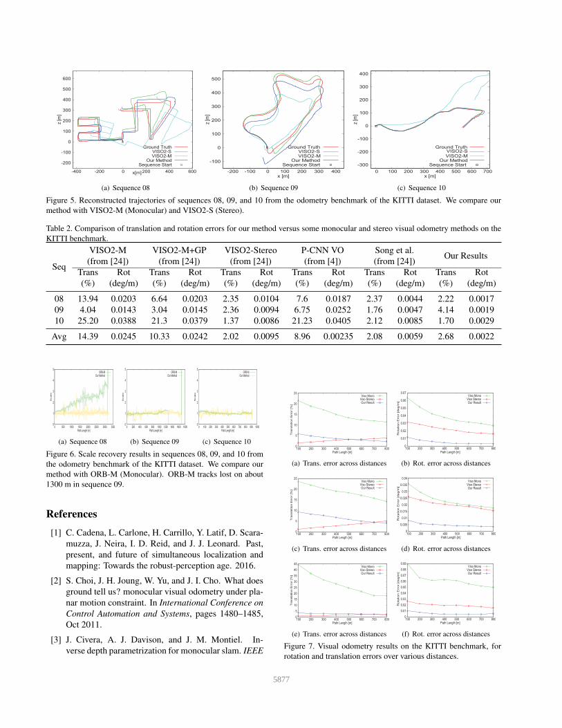
Figure 5 and 7 show the reconstructed trajectories and
errors in translation and rotation of VISO-M (Monocular),
VISO-S (Stereo) [9] and our method. Comparing with
VISO-S, we obtain a comparative performance in transla-
tion on sequence 08 and 10. Figure 5(a) shows that our
method is better than VISO-S for long distance driving. Ap-
parently, our method is much better than VISO-M method.
As for rotation estimation, our result is much better than
other methods’. And our rotation calculation is based on
that of ORB-SLAM method.
We also compare the performances of our method with
ORB-M (Monocular) SLAM as shown in Figure 6. The
scales are obtained by dividing the moving distances of con-
secutive frames to the ground truth. The expected value
would be 1. Zero means track lost, which means it can not
calculate the egomotion. From the results, we can find out
that our method can keep the scale from drift for long dis-
tance motion (3000 meters in sequence 08). ORB-M can
get a very good performance in calculating rotation. On the
other hand, it is facing a large scale drift problem. Loop
closure detection in ORB-SLAM can eliminate the scale
drift. If the loop closure detection fail, it will not get a
good performance for scale correction. Unlike the ORB
slam method, we do not include the close loop detection and
loop correction in our algorithm. Our method can also be a
good compensation for other monocular odometry methods
which are facing scale drift problem.
6. Conclusion
We present a novel scale recovery method for monocular
visual odometry. The scale of translation is obtained using
depth predicted from images, and depth is predicted with
convolutional neural fields. The performance of depth
prediction is improved by incorporating the consecutive
frames and egomotion into our networks. The advantage
of our method is that it can recover the scale and elimi-
nate the scale drift from structural information of whole
environments rather than from a fixed reference plane.
Experiments are conducted on the KITTI dataset to verify
the effectiveness of our method. The experimental results
show that our algorithm can improve the accuracy on both
visual odometry and depth estimation tasks.
Acknowledgements. We thank the anonymous review-
ers for their valable comments. This work is supported
in part by the National Natural Science Foundation of
China (61573260, 61673300), the Fundamental Research
Funds for the Central Universities, the Basic Research
Project of Shanghai Science and Technology Commis-
sion(16JC1401200, 16DZ1200903).
5876
-200
-100
0
100
200
300
400
500
600
-400 -200 0 200 400 600
z [m
]
V M
m]
Ground TruthV S
Our MethodSequence Start
(a) Sequence 08
-100
0
100
200
300
400
500
-200 -100 0 100 200 300 400
z [m]
x [m]
Ground TruthV SV M
Our MethodSequence Start
(b) Sequence 09
-300
-200
-100
0
100
200
300
400
0 100 200 300 400 500 600 700
z [m
]
x [m]
Ground TruthV SV M
Our MethodSequence Start
(c) Sequence 10
Figure 5. Reconstructed trajectories of sequences 08, 09, and 10 from the odometry benchmark of the KITTI dataset. We compare our
method with VISO2-M (Monocular) and VISO2-S (Stereo).
Table 2. Comparison of translation and rotation errors for our method versus some monocular and stereo visual odometry methods on the
KITTI benchmark.
Seq
VISO2-M VISO2-M+GP VISO2-Stereo P-CNN VO Song et al.Our Results
(from [24]) (from [24]) (from [24]) (from [4]) (from [24])
Trans Rot Trans Rot Trans Rot Trans Rot Trans Rot Trans Rot
(%) (deg/m) (%) (deg/m) (%) (deg/m) (%) (deg/m) (%) (deg/m) (%) (deg/m)
08 13.94 0.0203 6.64 0.0203 2.35 0.0104 7.6 0.0187 2.37 0.0044 2.22 0.0017
09 4.04 0.0143 3.04 0.0145 2.36 0.0094 6.75 0.0252 1.76 0.0047 4.14 0.0019
10 25.20 0.0388 21.3 0.0379 1.37 0.0086 21.23 0.0405 2.12 0.0085 1.70 0.0029
Avg 14.39 0.0245 10.33 0.0242 2.02 0.0095 8.96 0.00235 2.08 0.0059 2.68 0.0022
0
1
2
3
4
5
0 500 1000 1500 2000 2500 3000 3500
Scale
Path Length [m]
ORB-MOur Method
(a) Sequence 08
0
1
2
3
4
5
0 200 400 600 800 1000 1200 1400 1600 1800
Scale
Path Length [m]
ORB-MOur Method
(b) Sequence 09
0
1
2
3
4
5
0 100 200 300 400 500 600 700 800 900 1000
Scale
Path Length [m]
ORB-MOur Method
(c) Sequence 10
Figure 6. Scale recovery results in sequences 08, 09, and 10 from
the odometry benchmark of the KITTI dataset. We compare our
method with ORB-M (Monocular). ORB-M tracks lost on about
1300 m in sequence 09.
References
[1] C. Cadena, L. Carlone, H. Carrillo, Y. Latif, D. Scara-
muzza, J. Neira, I. D. Reid, and J. J. Leonard. Past,
present, and future of simultaneous localization and
mapping: Towards the robust-perception age. 2016.
[2] S. Choi, J. H. Joung, W. Yu, and J. I. Cho. What does
ground tell us? monocular visual odometry under pla-
nar motion constraint. In International Conference on
Control Automation and Systems, pages 1480–1485,
Oct 2011.
[3] J. Civera, A. J. Davison, and J. M. Montiel. In-
verse depth parametrization for monocular slam. IEEE
0
5
10
15
20
25
100 200 300 400 500 600 700 800
Tra
nsla
tion
Err
or [%
]
Path Length [m]
Viso MonoViso StereoOur Result
(a) Trans. error across distances
0
0.01
0.02
0.03
0.04
0.05
0.06
0.07
100 200 300 400 500 600 700 800
Err
or
[
Path Length [m]
Viso MonoViso StereoOur Result
(b) Rot. error across distances
0
5
10
15
20
25
100 200 300 400 500 600 700 800
Tra
nsla
tion
Err
or [%
]
Path Length [m]
Viso MonoViso StereoOur Result
(c) Trans. error across distances
0
0.005
0.01
0.015
0.02
0.025
0.03
0.035
0.04
100 200 300 400 500 600 700 800
Err
or
[
Path Length [m]
Viso MonoViso StereoOur Result
(d) Rot. error across distances
0
5
10
15
20
25
30
35
40
45
100 200 300 400 500 600 700 800
Tra
nsla
tion
Err
or [%
]
Path Length [m]
Viso MonoViso StereoOur Result
(e) Trans. error across distances
0
0.01
0.02
0.03
0.04
0.05
0.06
0.07
0.08
0.09
100 200 300 400 500 600 700 800
Err
or
[]
Path Length [m]
Viso MonoViso StereoOur Result
(f) Rot. error across distances
Figure 7. Visual odometry results on the KITTI benchmark, for
rotation and translation errors over various distances.
5877

transactions on robotics, 24(5):932–945, 2008.
[4] G. Costante, M. Mancini, P. Valigi, and T. A. Cia-
rfuglia. Exploring representation learning with cnns
for frame-to-frame ego-motion estimation. IEEE
Robotics and Automation Letters, 1(1):18–25, 2016.
[5] T. Dang, C. Hoffmann, and C. Stiller. Continuous
stereo self-calibration by camera parameter tracking.
IEEE Transactions on Image Processing, 18(7):1536–
1550, 2009.
[6] D. Eigen and R. Fergus. Predicting depth, surface nor-
mals and semantic labels with a common multi-scale
convolutional architecture. In Proceedings of the IEEE
International Conference on Computer Vision, pages
2650–2658, 2015.
[7] D. Eigen, C. Puhrsch, and R. Fergus. Depth map pre-
diction from a single image using a multi-scale deep
network. In Proceedings of Advances in Neural Infor-
mation Processing Systems, pages 2366–2374, 2014.
[8] A. Geiger, P. Lenz, and R. Urtasun. Are we ready
for autonomous driving? the kitti vision benchmark
suite. In Conference on Computer Vision and Pattern
Recognition, 2012.
[9] A. Geiger, J. Ziegler, and C. Stiller. Stereoscan: Dense
3d reconstruction in real-time. In Intelligent Vehicles
Symposium, 2011.
[10] K. He, X. Zhang, S. Ren, and J. Sun. Deep residual
learning for image recognition. In Computer Vision
and Pattern Recognition, pages 770–778, 2016.
[11] A. Hyvarinen. Estimation of non-normalized statis-
tical models by score matching. Journal of Machine
Learning Research, 6(Apr):695–709, 2005.
[12] K. Karsch, C. Liu, and S. B. Kang. Depth trans-
fer: Depth extraction from video using non-parametric
sampling. IEEE transactions on pattern analysis and
machine intelligence, 36(11):2144–2158, 2014.
[13] C. Kerl, J. Sturm, and D. Cremers. Robust odometry
estimation for rgb-d cameras. In IEEE International
Conference on Robotics and Automation, pages 3748–
3754. IEEE, 2013.
[14] K. L. Lange, R. J. Little, and J. M. Taylor. Robust
statistical modeling using the t distribution. Journal
of the American Statistical Association, 84(408):881–
896, 1989.
[15] B. Lee, K. Daniilidis, and D. D. Lee. Online self-
supervised monocular visual odometry for ground ve-
hicles. In 2015 IEEE International Conference on
Robotics and Automation, pages 5232–5238. IEEE,
2015.
[16] A. Levin, D. Lischinski, and Y. Weiss. Colorization
using optimization. In ACM Transactions on Graph-
ics, volume 23, pages 689–694. ACM, 2004.
[17] B. Li, C. Shen, Y. Dai, A. V. D. Hengel, and M. He.
Depth and surface normal estimation from monocular
images using regression on deep features and hierar-
chical crfs. pages 1119–1127, 2015.
[18] F. Liu, C. Shen, G. Lin, and I. Reid. Learning
depth from single monocular images using deep con-
volutional neural fields. IEEE Transactions on Pat-
tern Analysis and Machine Intelligence, 38(10):2024–
2039, Oct 2016.
[19] J. Long, E. Shelhamer, and T. Darrell. Fully convolu-
tional networks for semantic segmentation. In IEEE
Conference on Computer Vision and Pattern Recogni-
tion, pages 3431–3440, 2015.
[20] R. Mur-Artal, J. M. M. Montiel, and J. D. Tards. Orb-
slam: A versatile and accurate monocular slam sys-
tem. IEEE Transactions on Robotics, 31(5):1147–
1163, Oct 2015.
[21] R. Ranftl, V. Vineet, Q. Chen, and V. Koltun. Dense
monocular depth estimation in complex dynamic
scenes. 2016.
[22] A. Saxena, M. Sun, and A. Y. Ng. Make3d: learn-
ing 3d scene structure from a single still image. IEEE
Transactions on Pattern Analysis and Machine Intelli-
gence, 31(5):824–840, 2009.
[23] D. Scaramuzza and F. Fraundorfer. Visual odometry.
IEEE Robotics & Automation Magazine, 18(4):80–92,
2011.
[24] S. Song, M. Chandraker, and C. C. Guest. High ac-
curacy monocular sfm and scale correction for au-
tonomous driving. IEEE Transactions on Pattern
Analysis and Machine Intelligence, 38(4):730–743,
April 2016.
5878