Representative hydraulic conductivity of hydrogeologic units
Vanessa A. Godoy1,2*, Lázaro Valentin Zuquette1 and J. Jaime Gómez-Hernández2
1 Geotechnical Engineering Department, São Carlos School of Engineering, University of São
Paulo. Avenida Trabalhador São Carlense, 400, 16564-002, São Carlos, São Paulo, Brazil.
2 Institute for Water and Environmental Engineering, Universitat Politècnica de València, Camí de
Vera, s/n, 46022, València, Spain
* corresponding author: [email protected] (+55)16 35739501
Scale effect on hydraulic conductivity and solute transport: small and large-scale laboratory experiments and field experiments Highlights
• Hydraulic conductivity increases with scale for the same measurement condition. • Dispersivity increases with sample height following exponential functions. • Partition coefficient increases with sample support following linear functions. • The scale effect obtained can be explained by the soil heterogeneities. • To improve predictions reliability and accuracy, scale effect should be considered.
Abstract Hydraulic conductivity (K), dispersivity (α) and partition coefficient (Kd) can change according to
the measurement support (scale) and that is referred as scale effect. However, there is no clear
consensus about the scale behavior of these parameters. Comparison between results obtained
in different support of measurements in the field and in the laboratory can promote the discussion
about scale effects on K, α and Kd, and contribute to understanding how these parameters behave
with the change in the scale of measurement, the main objectives of the present paper. Small and
large-scale laboratory tests using undisturbed soil samples and field experiments at different
scales were performed. Results show that for the same measurement condition K, α and Kd
increase with scale, in all studied magnitudes. Caution should be taken when using K, α and Kd
values in numerical models with no concern about the scale effect. The lack of consideration of
the difference of scale between field and laboratory measurements and numerical model may
compromise the reliability of the predictions and misrepresent the responses.
Keywords: undisturbed soil sample, column experiment, double-ring infiltrometer, infiltration
ditch, tropical soil
1. Introduction
Numerical models are tools used in the geotechnical and geoenvironmental practice to solve
a wide range of problems related to water flow and solute movement in the subsurface (Dou et
al., 2014; Ghiglieri et al., 2016; Navarro et al., 2017; Wang et al., 2017). Hydraulic conductivity
(K) and the solute transport parameters such as hydrodynamic dispersion coefficient (D),
dispersivity (α), partition coefficient (Kd), and retardation factor (R) are key input parameters for
these numerical models and their proper determination is fundamental (Bouchelaghem and Jozja,
2009).
In common practice, these parameters are determined in the field or in the laboratory, and
then they are used in models to conduct predictions, with no concern about the scale (support) at
which they were measured (Godoy et al., 2015; Latorre et al., 2015; Liu et al., 2014). But the
value of these parameters can change according to the measurement support, and when that
change is not considered, the reliability of the predictions may be compromised (Godoy et al.,
2018; Sánchez-Vila et al., 1996). The dependence of parameter values on measurement support
is called scale effect, it is a result of the parameters spatial variability (Sánchez-Vila et al., 1996),
and it has been the subject of many studies (Salamon et al., 2007; Yang et al., 2017).
In the last decades, scale effects on mechanical properties relevant to geotechnical problems
have been studied (Bahaaddini et al., 2014; Yilmaz et al., 2015; Yoshinaka et al., 2008). However,
experimental studies of scale effects on K and solute transport parameters have received less
attention. Most experimental studies of scale effects in solute transport are related to α and have
shown that it increases with the scale (Domenico and Robbins, 1984; Gelhar and Axness, 1983;
Vik et al., 2013). Regarding K, some authors suggested that there is no scale effect and that the
differences in value at different scales are primarily due to problems during the measurements
and not due to its measurement support (Butler and Healey, 1998a, 1998b). However, many
studies have shown that K computed in the laboratory tend to have a smaller mean and a larger
variance than K observed in the field over larger scales (Chapuis et al., 2005; Clauser, 1992;
Sobieraj et al., 2004; Yang et al., 2017). In any case, scale effects may vary according to
measurements conditions, geological characteristics and the spatial correlation length of K in a
specific site (Neuman, 1994; Tidwell, 2006).
Undisturbed soil cores of a range of sizes have been used to evaluate the scale effects on D
and α (Khan and Jury, 1990; Parker and Albrecht, 1987). The scale effects on sorption parameters
such as R and Kd were studied numerically by some authors (Cassiraga et al., 2005; Gómez-

Hernández et al., 2006), however, experimental studies are rare, mainly due to the difficulty in
conducting large-scale reactive solute transport experiments. Most of the investigations in scale
effects on K compare small-scale laboratory tests (i.e., permeameter tests) with intermediate-
scale aquifer tests (i.e., slug tests), and with large-scale tests (i.e., pumping tests). In the
geotechnical and geoenvironmental practice the tests used to determine soil saturated K, such
as column experiment, double-ring infiltrometer and falling-head infiltration ditch, are rarely used
to analyze scale effects (Duong et al., 2013; Lai and Ren, 2007), resulting in a lack of knowledge
that we hope to contribute to reduce.
It is noticeable that there is no clear consensus as to the scale effect on water flow and solute
transport parameters. The main purpose of the present paper is to contribute to the discussion
about scale effects on K, α, and Kd and understanding how these parameters behave with the
change in the scale of measurement. For this, we characterized a study area and performed
small- and large-scale laboratory tests using undisturbed soil samples, and field experiments, at
different scales. The studied geologic material is a tropical soil that is widely found across the São
Paulo State in Brazil, and that was not been characterized yet in terms of scale effects on K, α,
and Kd.
2. Materials and methods
1.1. Basic description of the studied soil Field studies were carried out in the city of São Carlos (21°51′38″ S, 47°54′14″ W), located in
the East-Center of the São Paulo State, Brazil. Based on granulometric analyses with and without
deflocculant, depending on the flocculation of the soil’s grains, the soil is classified as CL or SF,
according to the Unified Soil Classification System (USCS). The geologic material studied
comprises Cenozoic sediments that cover the Botucatu Formation (Paraná Sedimentary Basin,
São Bento Group), constituted by unconsolidated sands with a thickness ranging from 5 m to 7
m and pebbles at the base, and are widely spread across São Paulo State (Giacheti et al., 1993).
Tropical conditions and wheatering make the soil from the Cenozoic sediments highly lateritized
(Giacheti et al., 1993). The main constituents of this soil are quartz, oxides,
and hydroxides of aluminum, kaolinite, and gibbsite. Macropores and dual-porosity are also
characteristics of this soil (Rohm, 1992).
1.2. Soil sampling and characterization Large- and small-scale undisturbed soil samples were taken from the bottom and slopes of
excavated ditches by carefully introducing rigid polyvinyl chloride (PVC) cylinders into the soil.
Small-scale samples were extracted in 23 locations in the x-y plane in an area of 12 m along the
x-direction and 7 m along the y-direction. For each x-y coordinate, three samples were taken at
three different depths: 0.5 m, 1.0 m, and 1.5 m resulting in a dense sampling design. A total of 14
small-scale samples were discarded because they presented defects or cracks. Large-scale
samples were taken in an area next to where the small-scale samples were taken, retaining only
those without defects. Table 1 shows the dimensions and number of undisturbed samples taken.
Disturbed soil samples were collected to perform routine physical, physico-chemical, chemical
and mineralogical characterization. Three replicates were used to determine the following
parameters by using disturbed soil samples: pH in H2O, pH in KCl, ΔpH (pHKCl – pHH2O) (Mekaru
and Uehara, 1972), point of zero charge (PZC) (2pHKCl – pHH2O) (Keng and Uehara, 1973), organic
matter (ASTM, 2014a), and mineralogical composition by X-ray diffraction (Azaroff and Buerger,
1953).
Next, we describe the analyses performed for each of the small- and large-scale undisturbed
soil samples. At the laboratory, dry density was determined as ρd = Md/Vt, where Vt is the total
volume of the soil sample (internal volume of each PVC cylinder) and Md is the dry mass of the
soil sample (Knappett and Craig, 2012). Total porosity was calculated as n=1 – ρd/ρs, where ρs is
the particle density, determined using the ASTM D 854-14 (ASTM, 2014b) as 2.71 Mg·m-3
(Knappett and Craig, 2012). Mercury intrusion porosimetry (MIP) (Washburn, 1921) was
performed and used to determine macroporosity (Ma), mesoporosity (Me), and microporosity (Mi)
according to the classification proposed by Koorevaar et al. (1983), in which the diameters of Mi,
Me, and Ma are <30 µm, 30-100 µm and >100 µm, respectively. Disturbed samples were taken
from each one of the undisturbed samples and were air-dried and sieved through a #10 mesh
sieve (2 mm openings). Particle size distributions were determined according to ASTM D7928-17
(ASTM, 2017a) and ASTM D6913 / D6913M-17 (ASTM, 2017b). The methylene blue adsorption
test using the filter paper method described by Pejon (1992) was used to determine the cation
exchange capacity (CEC).
1.3. Large- and small-scale column experiments The characteristics of the flow and transport laboratory experiments were the same for both
small and large-scale experiments to allow the comparison between them. We used the PVC

cylinders filled with undisturbed soil samples as rigid-wall permeameters and small- and large-
scale column experiments were conducted as follows. First, the soil samples were slowly
saturated from the bottom with deionized water to remove possible entrapped air. And second,
after column saturation, flow was reversed (now from top to bottom) and a column test was
performed under a constant hydraulic gradient of 1; the flow rate (Q) was measured. We took two
measures per day for two weeks and we assumed that steady-state flow was achieved when Q
variations were below 5% in four consecutive measurements. Once steady-state was reached,
we determined saturated hydraulic conductivity, K, specific discharge, q, and average linear
velocity, v (q/ne) (Freeze and Cherry, 1979), where ne is the effective porosity, which was
calculated as the total porosity minus the porosity that corresponds to the soil water content at 33
kPa (suction equivalent to the soil field capacity) (Ahuja et al., 1984). After that, deionized water
was substituted by a solution 2.56 mol m-3 KCl composed by 100 mg L-1 K+ and 90.7 mg L-1 Cl-,
referred to, later on, as the initial concentration, C0. Solute displacement tests were carried out
under constant hydraulic head and isothermal (20 °C) conditions. Leachate samples were
collected from the outlet of the columns and concentrations (C) were measured at preset time
intervals. An ion-selective electrode (ISE) (Hanna instruments - HI 4107 model) was used to
determine the Cl- concentration. We used a flame photometer (Micronal B462 model) to measure
the K+ concentration at a 1:21 dilution ratio. The concentrations of the ions were measured two
times for each sample and the arithmetic mean of the measures was used as the final value.
The breakthrough curves (BTC’s) were given as C/C0 vs. the number of pore volumes (T)
injected. T is a dimensionless variable calculated as T = vt/L (van Genuchten, 1980), where v is
the average linear velocity, t is the time elapsed from the start of the solute application, and L is
the length of the soil column.
The transport parameters, dispersivity (α) [L] and partition coefficient between the liquid and
solid phases (Kd) [L³M- 1] were also determined as explained next.
The advection-dispersion equation (ADE) (Freeze and Cherry, 1979) used to interpret the
BTCs is
R ∂C∂t =D
∂2C∂x2 -v
∂C∂x ,
(1)
where C is solute concentration [ML-3], D is the hydrodynamic dispersion coefficient [M2T-1], R is
the retardation factor [-], x is distance [L], and t is time [T].
The hydrodynamic dispersion coefficient is related to the α by (Freeze and Cherry, 1979)
D= α·v, (2)
and the retardation factor is related to the Kd through the expression (Freeze and Cherry, 1979)
R= 1+ρdn Kd. (3)
The ADE has the following analytical solution (Lapidus and Amundson, 1952) when the initial
condition is C (x,0) = 0 for the entire sample, and the boundary conditions are C=C0 at the inlet
and C=0 at an infinite distance from the inlet
CC0
=12$erfc %
RL-vt2√DRt
'(+12 exp %
vLD 'erfc %
RL+vt2√DRt
', (4)
where erfc is the complementary error function.
This expression was fitted to the observed BTCs for each soil sample and values of D and R
were obtained for both K+ and Cl-. The fitting was performed using the computer program CFITM
(van Genuchten, 1980), that is part of the Windows-based computer software package Studio
of Analytical Models (STANMOD) (Šimůnek et al., 1999). The fit of the experimental BTC to the
ADE model was evaluated by its R2. Most BTCs presented significant tailing, R2 ranged from 0.77
to 0.99 with a mean of 0.92. We conclude that the ADE model is suitable to describe the
experimental data.
From the values of D and R obtained after the fitting, the values of the α and the Kd were
calculated using Eq. (2) and (3), respectively.
1.4. Field experiments Following, field experiments are described. Notice that solute transport experiments were not
conducted in the field, only flow experiments.
i.Double-ring infiltrometer (DRI)
In the study area, seven double-ring infiltrometer tests (DRI) were conducted according to
ASTM D3385-118 (ASTM, 2018). The DRIs used are made up of two concentric stainless-steel
rings, with diameters of 0.30 m and 0.60 m. The height of water in the inner ring was 0.15 m in all
tests. The water level in a Mariotte tube was measured at preset time intervals. The DRI
experiments were carried out until steady-state flow was reached, that is when discharge changes
were < 0.5% over a 5-minute interval. The duration of the tests ranged between 135 and 192
minutes. The infiltration rate was calculated on the basis of the observations. Empirical relations

show that the infiltration rate decreases with time and tends to an asymptotic value, generally
equal to the K (Fatehnia et al., 2016).
ii.Infiltration in rectangular ditches
The infiltration in rectangular ditches was done by using the modified inversed auger-hole
method (Porchet’s method) proposed by Stibinger (2014). According to this method, we used
rectangular infiltration ditch with width a [L] and length b [L]. The total infiltration flow (through the
bottom and sides of the ditch) [L3T-1] can be measured by the variation in time of the volume of
water in the ditch. If the water level is h, the volume water in the ditch is given by
V=a b h , (5)
and, since width and length do not change in time, the infiltration flow results
Q=(ab)dhdt .
(6)
Assuming that the distance from the bottom of the ditch to the wetting front is large compared
to the initial water level in the ditch (h0), then the hydraulic gradient approximates unity. In which
case, if the Darcy Law is valid and the wetted soil below the ditch is practically saturated, the flux
in the wetted soil approaches its K.
Total infiltration (TI) in the ditch can be expressed as the sum of the infiltration through the
bottom and the infiltration through the sides
TI=BI+WI. (7)
The total area through which flow occurs is the sum of the bottom area (ab) plus the area on
the sides (2ah+2bh). Darcy’s law states that total flow is Q=- K i A, where i is the hydraulic gradient
(equal to one in our case), and A is the flowing area, therefore,
BI+WI= -(ab+2(a+b)h)K, (8)
where the negative sign indicates that the z-axis is positive upwards, but water flow is downwards.
By combining Eq. (6) and (8), we obtain
(ab)dhdt =-(ab+2(a+b)h)K, (9)
which, after integration, yields
K+tm-tj,= -ab
2(a+b) ln .hm+ ab
2(a+b)
hj+ab
2(a+b)
/, (10)
where hj is the water level at time tj and hm is the water level at time tm.
Eq. (10) can be rewritten by substituting B = ab/2(a+b)
K+tm-tj,= -Bln 0hm+Bhj+B
1, (11)
Replacing h0 for t0=0, the equation results
Kt*= -Bln 2h*+Bh4+B
5, (12)
where h* is the water level at time t*, from which the expression of the evolution of water level
with time is
h*= h0+B
exp Kt*B
-B, (13)
K can de deduced from the fitting of Eq. (13) to the observed water level decline in time.
We conducted falling-head infiltration tests in rectangular ditches of 0.70 m width by 0.40
m depth and five different lengths: 1 m, 2 m, 4 m, 6 m, and 8 m. All tests were performed twice
with an interval of two weeks between the first and the second test. Before starting the
measurements, the soil was saturated by continuously introducing water for one hour, using a
water truck. The initial water height in the ditch, h0, was set to 0.19 m for all ditches. Total infiltration
time ranged from 60 to 90 minutes. Non-linear regression analysis using MATLAB function
lsqcurvefit was used to fit Eq. (13) to the data and to determine the value of K. Water evaporation
was measured and the infiltration flow was corrected when necessary.
1.5. Results and discussion
iii.Soil characterization
The physical characterization of the 55 small-scale undisturbed soil samples is summarized
in statistical terms in Table 2. It is noticeable that the soil presents a significant variability (Wilding
and Drees, 1983) for some properties such as macroporosity and silt content. Our results confirm
that soil heterogeneity is present even on a small scale (Chapuis et al., 2005). Properties such as
porosity and dry density were more homogeneous and presented only a small variability. The
highest percentages of pore diameters found in the soil correspond to mesoporosity and
microporosity. The multimodal pore size distribution is characteristic of well-structured soils
(Lipiec et al., 2007) and can influence water flow and solute transport in these soils. Fig. 1 shows
the results of three MIP tests performed with samples taken at 0.5 m, 1.0 m, and 1.5 m depth:
dual-porosity is evident.
Regarding the granulometric analyses, when the soil sample was prepared with deflocculant
the soil is texturally classified as a clayey fine sand. But when the soil was analyzed in its natural
condition, that is, no deflocculant was used, its texture is completely different, resulting in a
coarser textural class. This behavior indicates the presence of aggregates in the soil, a
characteristic of lateritic soils that can play an important role in water flow and solute transport.
We also obtained a low CEC of 4.20 cmolc Kg-1, indicative of a soil with low capacity to adsorb
cations by electrostatic adsorption (Fagundes and Zuquette, 2011). Finally, the mean values of
the soil physical properties were in accordance with typical values found earlier in this type of soil
(Giacheti et al., 1993).
To better understand the solute transport results, soil mineralogy, physico-chemical and
chemical properties were also investigated. According to results of the X-ray diffraction, the main
minerals present in the soil are quartz, kaolinite, and gibbsite. The soil can be considered as
strongly acidic, with average values of 5.71 and 5.19 for pH in H2O and in KCl, respectively.
Cenozoic sediments and lateritic soils are commonly acidic (Giacheti et al., 1993). Important
properties related to solute transport are the negative ΔpH (-0.52) and the point of zero charge
(PZC) (4.67) that indicates a predominance of negative charges, resulting in important cation
adsorption (Fagundes and Zuquette, 2011). The average of the amount of organic matter was
small (2.40%), result in accordance with lateritic acid soils.
iv.Evaluation of the scale dependence in the hydraulic conductivity
Basic statistics of K were inferred from the 55 small-scale column experiments obtaining mean
and standard deviation (SD) of 1.35 m/d and 1.65 m/d, respectively. The coefficient of variation
(CV) was 1.22 and indicates a highly variable parameter (Wilding and Drees, 1983). We expect
scale effects since these are mostly related to the degree of heterogeneity (Sánchez-Vila et al.
1996).
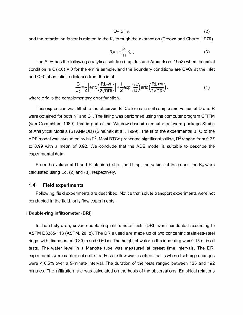
The mean K values obtained from the large-scale column experiments were calculated for
each set of samples. Previous studies have shown that scale effects are dependent on the sample
volume (Al-Raoush and Papadopoulos, 2010; Valdés-Parada et al., 2012). But, before analyzing
that dependence, we have analyzed if there are scale effects associated with the column height
or the column diameter. Fig. 2 (A-B) shows the variation of K with column height and diameter.
Average K values ranged between 1.35 m/d and 2.1 m/d. These differences can be considered
moderate for water flow modeling, but they can be significant for solute transport predictions.
Average K increased with the sample diameter. K seems to increase with height, except for the
samples with a diameter of 0.2 m, for which no clear trend was verified. Only a small range of
diameters and heights were analyzed in this research, so these results should be taken as only
indicative.
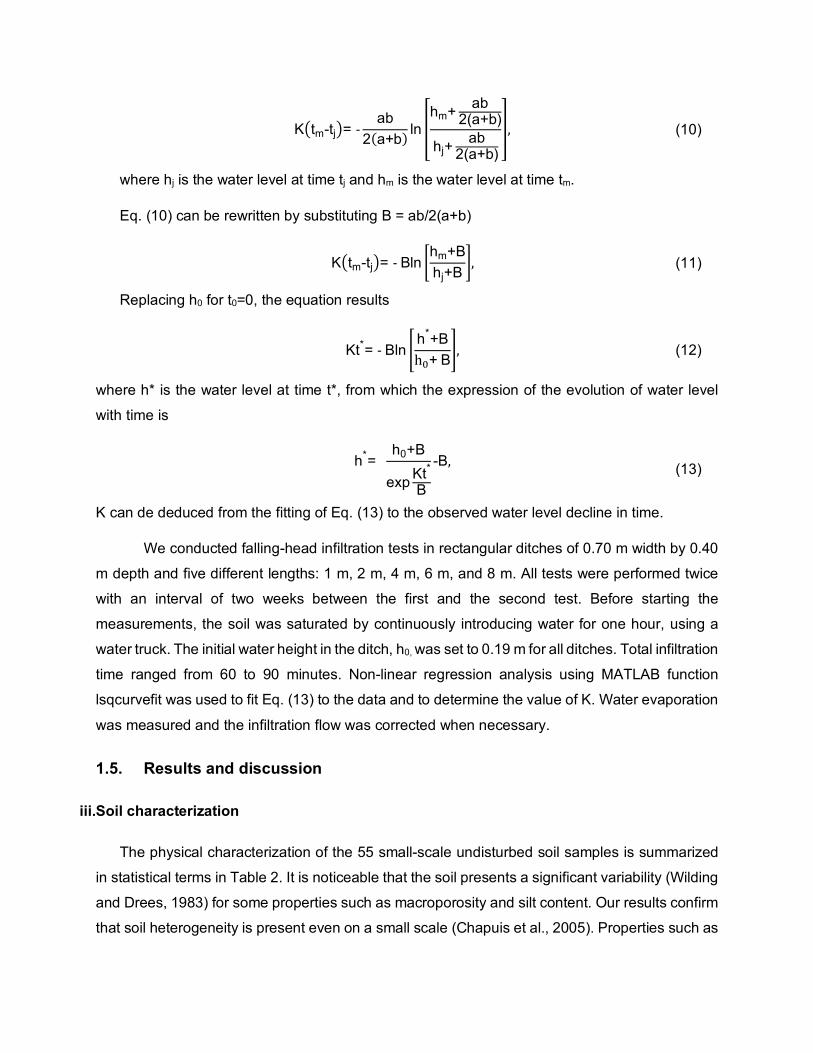
Fig. 3 (A-B) shows the infiltration rate as a function of time for seven double-ring infiltrometer
tests. We can see that all tests behave similarly, although they have very different transition
zones. The infiltration rate decreases rapidly at the beginning of the test, as expected due to high
potential differences, then it tends to a limiting value that can be assimilated to the soil K. Double-
ring infiltrometer tests resulted in K values ranging from 0.104 m/d to 0.538 m/d, with a mean
value equal to 0.36 m/d, SD is equal to 0.147 m/d and the CV is 0.45, showing a moderate
heterogeneity that, as discussed before, is present at all scales. Fig. 3B is a zoom in Fig. 3A to
show the transition zones, where the greatest variability happens.
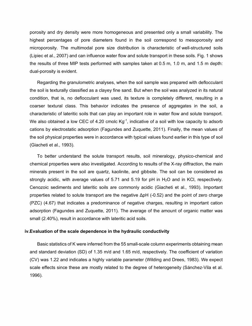
Fig. 4 shows the reduction of the water table with time in the two tests performed in each ditch.
From these curves, K was determined using Eq. (13). Very similar results were obtained for each
pair of tests performed in the same ditch. It is possible to see that the slope of the curves increases
as the ditch length increases, indicating that the water level lowers faster as the test scale
increases and, therefore, the K for the test tends to increase, with the exception of the ditch of
4 m length, which has the smallest slope. K values ranged from 1.44 m/d to 6.04 m/d, with a mean
equal to 2.7 m/d and a SD of 1.68 m/d.
The scale effect on K was evaluated by analyzing the K values against the sample support,
that is, against the volume of the sample for which K was evaluated. For the small-scale samples,
the sample volume is simply the permeameter volume, and for the DRI and the ditches, the
sample support was the volume of saturated soil. The depth of the saturated zone was determined
by taking soil samples every 0.2 m, immediately after the tests, to determine the soil moisture.
The average saturated depth of all tests was 0.5 m and this value was used in the calculation of
the volume of saturated soil.

Fig. 5 (A-C) shows the variation of K with sample volume. According to these results, K seems
to increase with scale, despite some oscillations. Laboratory tests were performed after the
removal of entrapped air, that can reduce in the K, by slowly saturate the samples from the bottom.
However, in the field tests, the removal of the entrapped air cannot be assured, although soil
saturation before the ditches infiltration tests. This can justify the results obtained for the DRI tests
that give mean K value lower than that obtained at the laboratory, even though the volume of DRI
sample is bigger than the volume of sample used in the laboratory experiments (Fig 5 A). We are
aware that laboratory and field experiments were not performed at the same conditions and
comparisons between such data from different test conditions cannot be appropriate and the
results obtained from laboratory and field test are then show separately. Fig. 5B shows the results
only for the laboratory tests and Fig. 5C shows the results only for the field tests. In these figures,
we can see for each test condition, K increases with the sample volume. Similar results were also
observed by other researchers (Chapuis et al., 2005; Lai and Ren, 2007; Sobieraj et al., 2004;
Tidwell, 2006) who attribute it to the high K features that are not present at small scales. We
conclude that, for the same measurement condition, there is scale effect on K since observed K
values depend on the volume sampled. In general, the K obtained at the laboratory were lower
than that obtained at the field, however, these results cannot be conclusive since the difference
in test conditions can influence the responses (Neuman, 1994; Tidwell, 2006).
The variation of the K with the sample volume must be taken into account when these
observations are later used as input to numerical models. The numerical model must be
constructed with elements of a size similar to that at which the data were collected, otherwise,
some upscaling rule must be used when observation and model scales are different (Huang and
Griffiths, 2015; Li et al., 2011).
v.Evaluation of the scale dependence in the transport parameters
Dispersivity and partition coefficient for Cl- and K+ from 55 miscible displacements tests in
small-scale undisturbed soil samples were determined, and their values are summarized in
Table 3. These parameters display high variability as a consequence of its heterogeneity (Alletto
and Coquet, 2009; Sánchez-Vila et al., 1996). The cation (K+) Kd were greater than the anion (Cl-)
ones, in agreement with the soil characteristics that do not favor anion adsorption, given the low
amount of organic matter and the negative charges in the surface of the soil particles. Fig. 6A-C
show BTCs of K+ and Cl- obtained experimentally for some of the small and large soil samples
studied.

The cation α values were also higher than the anion ones. These results are illustrated in
Fig. 6A where experimental BTCs of K+ and Cl- obtained in two of the 55 miscible displacement
tests are shown. K+ moves slower than Cl-, resulting in larger R and Kd. The fitted values for the
Kd are high, even for Cl-, which is a nonreactive solute. Since the mineralogical and
physicochemical characteristics of the soil cannot justify high R values, we argue that the soil
structure and other physical characteristics, such as dual-porosity and particle aggregates, are
playing an important role in the retention. For example, small pores can favor the formation of
immobile domains where mass can temporarily be trapped, decreasing its velocity, in relation to
the velocity of the flow, and increasing its R (Dousset et al., 2007; Jarvis, 2007; Silva et al., 2016).
The statistics of α and Kd for K+ and Cl- derived from the analysis of large-scale miscible
displacements tests are shown in Tables 4 and 5. These results agree with those obtained in
small-scale experiments and display high variability. As in the small-scale tests, mean values for
K+ were greater than those for Cl-. From these tables, it is noticeable that Cl- Kd are smaller than
those for K+ and, therefore, moves faster than K+. Fig. 6B and Fig. 6C shows, for each sample
size, BTCs of K+ and Cl-, respectively, for one of the tests. The S shape of the BTCs is also
indicative of the important role that dispersion plays as a transport mechanism in the studied soil,
which can be readily related to small-scale heterogeneity (Gerritse, 1996).
Fig. 7 shows how α varies as a function of the sample height (that is, length in the solute
transport direction), diameter and volume. As expected (Fetter, 1999; Freeze and Cherry, 1979),
dispersivities tend to increase with the scale, and this trend can be fitted with the following
exponential functions: α = 0.12 e 2.55x (R2 0.95) for K+ and α = 0.05 e 3.52x (R2 0.93) for Cl-. This
behavior can be attributed to heterogeneous arrangements in the soil sample since at larger
scales a larger number of heterogeneities can be found inducing a higher α. Gelhar (1987)
postulated that longitudinal dispersivity should initially increase linearly with distance and
eventually reach a constant asymptotic value. Gelhar and Axness (1983) concluded that α is
related to the distance through the expression α=0.1x, where x is the travel distance. Later, Gelhar
et al. (1992) observed that the linear relationship between α and travel distance should be
reconsidered. Vik et al. (2013) found a linear relation between α and distance, but their data
resulted in a lower slope (α=0.07x) than the one suggested by Gelhar and Axness’ expression.
Xu and Eckstein (1995) studied some regression formulas relating α and distance, and defined a
relationship between α and field scale in the form α = 0.83 [log x]2.414 and mentioned that the slope
of the curve approaches zero when the scale exceeds 1 km. Regarding the dependency of α with
sample diameter and sample volume, the results in Fig. 7 show no clear dependence and the
oscillations of data prevented a good fit by simple monotonic functions, with R 2 below 0.05 when
attempting to fit α to sample diameter. When trying to fit a monotonic function of α as a function
of sample volume, the R2 equals 0.4 and 0.3 for K+ and Cl-, respectively. From a practical point of
view, these results should serve as a cautionary note about routinely adopting α from a linear
regression without further considerations; otherwise, excessively large or small dilution may be
induced in solute transport predictions, and the environmental responses misrepresented.
Fig. 8 shows how Kd varies as a function of the sample height (length in the solute transport
direction), diameter and volume. The Kd of K+ tends to increase with length, diameter and volume
(most clearly with the latter one), and the same can be said for the Kd of Cl-. On one hand, the fit
of Kd to sample height is poor for both K+ and Cl-, with R2 of 0.19 and 0.08, respectively. On the
other hand, Kd displays a clear trend as a function of sample diameter, which can be fitted with
the following functions: Kd = 14.2 x0.40 (R2 0.81) for K+, and Kd = 2.43 ln(x)+8.13 (R2 0.82) for Cl-,
where x is the dependent variable (height, diameter or volume of the sample). In addition, Kd also
displays a clear trend with sample volume, with the following linear functions: Kd = 158x+5.2 (R2
0.95) for K+ and Kd = 124x+2.3 (R2 0.70) for Cl-. With these results, it is noticeable that Kd of K+
and Cl- do not reach a stable value with any of the dimensions studied here. The clear
dependence on sample volume can be explained for the larger number of sorption sites as the
volume increases together with the larger heterogeneity of those sites.
1.6. Conclusions Small and large-scale laboratory experiments and field experiments were performed in order
to study scale effects on hydraulic conductivity (K), dispersivity (α) and partition coefficient (Kd) in
a tropical soil from Brazil. The studied soil was characterized in detail. Small and large-scale
undisturbed soil samples were used to perform column experiments to determine K, α, and Kd.
Seven-double ring infiltrometer tests and five infiltration tests in rectangular ditches were also
done to determine K.
The soil has dual-porosity and contains aggregates, a characteristic of lateritic soils that
probably played an important role in the soil K, α and Kd values. Due to its low CEC, the soil has
a low capacity to adsorb cations by electrostatic adsorption. However, the predominance of
negative charges in the soil particles surface favored cation adsorption. The coefficients of
variation obtained in all laboratory and field tests indicated that K, α, and Kd are highly
heterogeneous at all scales. In agreement with the soil characteristics, the cation (K+) Kd and α
were greater than the anion (Cl-) ones. From the BTCs it is clear that Cl- moves faster than K+.
The fitted values for the Kd are high, even for Cl-, which is considered a nonreactive solute. We
attribute that result to the soil structure and physical characteristics.
Average K increased with sample support, for the same measurement condition, result
attributed to the high heterogeneity and the high K features that are present in large scales but
not at small scales. K+ and Cl- α increases with travel distance, a behavior that can be fitted with
exponential functions. We attribute this trend to heterogeneous arrangements in the soil sample
since at larger scales there exist larger heterogeneities that induce higher α. The results show
that both the Kd of K+ and Cl- tend to increase in all studied magnitudes. We argue that these
results are due to the larger number of sorption sites as the sample support increases together
with the larger heterogeneity of those sites.
Finally, this paper warns against the use of the K, α, and Kd in numerical models with no
concern about the scale at which they were measured; not accounting for the difference of scale
between observation and model may distort the predictions and compromise their reliability.

Acknowledgments
The authors thank the financial support by the Brazilian National Council for Scientific and
Technological Development (CNPq) (Project 401441/2014-8). The doctoral fellowship awarded
to the first author by the Coordination of Improvement of Higher Level Personnel (CAPES) is
gratefully acknowledged. The first author also thanks to the international mobility grant awarded
by CNPq, through the Science Without Borders program (grant number: 200597/2015-9), and the
international mobility grant awarded by Santander Mobility in cooperation with the University of
São Paulo.

Bibliography
Ahuja, L.R., Naney, J.W., Green, R.E., Nielsen, D.R., 1984. Macroporosity to Characterize Spatial
Variability of Hydraulic Conductivity and Effects of Land Management1. Soil Sci. Soc. Am.
J. 48, 699. doi:10.2136/sssaj1984.03615995004800040001x
Al-Raoush, R., Papadopoulos, A., 2010. Representative elementary volume analysis of porous
media using X-ray computed tomography. Powder Technol. 200, 69–77.
doi:10.1016/j.powtec.2010.02.011
Alletto, L., Coquet, Y., 2009. Temporal and spatial variability of soil bulk density and near-
saturated hydraulic conductivity under two contrasted tillage management systems.
Geoderma 152, 85–94. doi:10.1016/j.geoderma.2009.05.023
ASTM, 2018. ASTM D3385 - 18, Standard Test Method for Infiltration Rate of Soils in Field Using
Double-Ring Infiltrometer.
ASTM, 2017a. ASTM D7928-17, Standard Test Method for Particle-Size Distribution (Gradation)
of Fine-Grained Soils Using the Sedimentation (Hydrometer) Analysis.
ASTM, 2017b. ASTM D6913 / D6913M-17, Standard Test Methods for Particle-Size Distribution
(Gradation) of Soils Using Sieve Analysis. doi:10.1520/D6913_D6913M-17
ASTM, 2014a. ASTM D2974 - 14, Standard Test Methods for Moisture, Ash, and Organic Matter
of Peat and Other Organic Soils. doi:10.1520/D2974-14
ASTM, 2014b. ASTM D854 - 14, Standard Test Methods for Specific Gravity of Soil Solids by
Water Pycnometer. doi:10.1520/D0854-14
Azaroff, L., Buerger, M., 1953. The powder method in X-ray crystallography. New York. McGraw-
Hill Book Co.
Bahaaddini, M., Hagan, P.C., Mitra, R., Hebblewhite, B.K., 2014. Scale effect on the shear
behaviour of rock joints based on a numerical study. Eng. Geol. 181, 212–223.
doi:10.1016/j.enggeo.2014.07.018
Bouchelaghem, F., Jozja, N., 2009. Multi-scale study of permeability evolution of a bentonite clay
owing to pollutant transport. Eng. Geol. 108, 286–294. doi:10.1016/j.enggeo.2009.06.021
Butler, J.J., Healey, J.M., 1998a. Relationship Between Pumping-Test and Slug-Test Parameters:
Scale Effect or Artifact? Ground Water 36, 305–312. doi:10.1111/j.1745-
6584.1998.tb01096.x

Butler, J.J., Healey, J.M., 1998b. Authors’ Reply. Ground Water 36, 867–868. doi:10.1111/j.1745-
6584.1998.tb02092.x
Cassiraga, E.F., Fernàndez-Garcia, D., Gómez-Hernández, J.J., 2005. Performance assessment
of solute transport upscaling methods in the context of nuclear waste disposal. Int. J. Rock
Mech. Min. Sci. 42, 756–764. doi:10.1016/j.ijrmms.2005.03.013
Chapuis, R.P., Dallaire, V., Marcotte, D., Chouteau, M., Acevedo, N., Gagnon, F., 2005.
Evaluating the hydraulic conductivity at three different scales within an unconfined sand
aquifer at Lachenaie, Quebec. Can. Geotech. J. 42, 1212–1220. doi:10.1139/t05-045
Clauser, C., 1992. Permeability of crystalline rocks. Eos, Trans. Am. Geophys. Union 73, 233–
233. doi:10.1029/91EO00190
Domenico, P.A., Robbins, G.A., 1984. A dispersion scale effect in model calibrations and field
tracer experiments. J. Hydrol. 70, 123–132. doi:10.1016/0022-1694(84)90117-3
Dou, H., Han, T., Gong, X., Zhang, J., 2014. Probabilistic slope stability analysis considering the
variability of hydraulic conductivity under rainfall infiltration–redistribution conditions. Eng.
Geol. 183, 1–13. doi:10.1016/j.enggeo.2014.09.005
Dousset, S., Thevenot, M., Pot, V., Šimunek, J., 2007. Evaluating equilibrium and non-equilibrium
transport of bromide and isoproturon in disturbed and undisturbed soil columns. J. Contam.
94, 261–276. doi:10.1016/j.jconhyd.2007.07.002
Duong, T. V., Trinh, V.N., Cui, Y.J., Tang, A.M., Calon, N., 2013. Development of a Large-Scale
Infiltration Column for Studying the Hydraulic Conductivity of Unsaturated Fouled Ballast.
Geotech. Test. J. 36, 20120099. doi:10.1520/GTJ20120099
Fagundes, J.R.T., Zuquette, L.V., 2011. Sorption behavior of the sandy residual unconsolidated
materials from the sandstones of the Botucatu Formation, the main aquifer of Brazil. Environ.
Earth Sci. 62, 831–845. doi:10.1007/s12665-010-0570-y
Fatehnia, Tawfiq, K., Ye, M., 2016. Estimation of saturated hydraulic conductivity from double-
ring infiltrometer measurements. Eur. J. Soil Sci. 67, 135–147. doi:10.1111/ejss.12322
Fetter, C., 1999. Contaminant hydrogeology, 2nd ed. Prentice Hall, New York.
Freeze, R., Cherry, J., 1979. Groundwater (p. 604). PrenticeHall Inc Englewood cliffs, New
Jersey.
Gelhar, L.W., Axness, C.L., 1983. Three-dimensional stochastic analysis of macrodispersion in
aquifers. Water Resour. Res. 19, 161–180. doi:10.1029/WR019i001p00161
Gelhar, L.W., Welty, C., Rehfeldt, K.R., 1992. A critical review of data on field-scale dispersion in
aquifers. Water Resour. Res. 28, 1955–1974. doi:10.1029/92WR00607
Gerritse, R.G., 1996. Dispersion of cadmium in columns of saturated sandy soils. J. Environ. Qual.
25, 1344–1349.
Ghiglieri, G., Carletti, A., Da Pelo, S., Cocco, F., Funedda, A., Loi, A., Manta, F., Pittalis, D., 2016.
Three-dimensional hydrogeological reconstruction based on geological depositional model:
A case study from the coastal plain of Arborea (Sardinia, Italy). Eng. Geol. 207, 103–114.
doi:10.1016/j.enggeo.2016.04.014
Giacheti, H.L., Rohm, S.A., Nogueira, J.B., Cintra, J.C.A., 1993. Geotechnical properties of the
Cenozoic sediment (In protuguese), in: Albiero, J.H., Cintra, J.C.A. (Eds.), Soil from the
Interior of São Paulo. ABMS, Sao Paulo, pp. 143–175.
Godoy, V.A., Valentin Zuquette, L., Gómez-Hernández, J.J., 2018. Stochastic analysis of three-
dimensional hydraulic conductivity upscaling in a heterogeneous tropical soil. Comput.
Geotech. 100, 174–187. doi:10.1016/j.compgeo.2018.03.004
Godoy, V.A., Zuquette, L.V., Napa-García, G.F., 2015. Hydrodynamic dispersion coefficient of
ammonium in undisturbed soil columns, in: Geotechnical Engineering for Infrastructure and
Development. ICE publishing, pp. 2699–2703.
Gómez-Hernández, J.J., Fu, J., Fernandez-Garcia, D., 2006. Upscaling retardation factors in 2-
D porous media, in: Bierkens, M.F.P., Gehrels, J.C., Kovar, K. (Eds.), Calibration and
Reliability in Groundwater Modelling : From Uncertainty to Decision Making : Proceedings of
the ModelCARE 2005 Conference Held in The Hague, the Netherlands, 6-9 June, 2005.
IAHS Publication, pp. 130–136.
Huang, J., Griffiths, D.V., 2015. Determining an appropriate finite element size for modelling the
strength of undrained random soils. Comput. Geotech. 69, 506–513.
doi:10.1016/j.compgeo.2015.06.020
Jarvis, N.J., 2007. A review of non-equilibrium water fl ow and solute transport in soil macropores:
Principles, controlling factors and consequences for water quality. Eur. J. Soil Sci. 58, 523–
546. doi:10.4141/cjss2011-050
Keng, J.C., Uehara, G., 1973. Chemistry, mineralogy, and taxonomy of oxisols and ultisols. Proc.
Soil Crop Sci. Soc. Florida 33, 119–926.
Khan, A.U.-H., Jury, W.A., 1990. A laboratory study of the dispersion scale effect in column

outflow experiments. J. Contam. Hydrol. 5, 119–131. doi:10.1016/0169-7722(90)90001-W
Knappett, J., Craig, R.F., 2012. Craig’s Soil Mechanics, 8th ed. CRC Press.
Koorevaar, P., Menelik, G., Dirksen, C., 1983. Elements of Soil Physics, 1st ed, Developments in
Soil Science. Elsevier Science. doi:10.1016/S0166-2481(08)70048-5
Lai, J., Ren, L., 2007. Assessing the Size Dependency of Measured Hydraulic Conductivity Using
Double-Ring Infiltrometers and Numerical Simulation. Soil Sci. Soc. Am. J. 71, 1667.
doi:10.2136/sssaj2006.0227
Lapidus, L., Amundson, N., 1952. Mathematics of adsorption in beds VI. The effect of longitudinal
diffusion in ion exchange and chromatographic columns. J. Phys. Chem. 984–988.
doi:10.1021/j150500a014
Latorre, B., Peña, C., Lassabatere, L., Angulo-Jaramillo, R., Moret-Fernández, D., 2015. Estimate
of soil hydraulic properties from disc infiltrometer three-dimensional infiltration curve.
Numerical analysis and field application. J. Hydrol. 527, 1–12.
doi:10.1016/j.jhydrol.2015.04.015
Li, L., Zhou, H., Gómez-Hernández, J.J., 2011. A comparative study of three-dimensional
hydraulic conductivity upscaling at the macro-dispersion experiment (MADE) site, Columbus
Air Force Base, Mississippi (USA). J. Hydrol. 404, 278–293.
doi:10.1016/j.jhydrol.2011.05.001
Lipiec, J., Walczak, R., Witkowska-Walczak, B., Nosalewicz, A., Słowińska-Jurkiewicz, A.,
Sławiński, C., 2007. The effect of aggregate size on water retention and pore structure of
two silt loam soils of different genesis. Soil Tillage Res. 97, 239–246.
doi:10.1016/j.still.2007.10.001
Liu, J., Huang, X., Liu, J., Wang, W., Zhang, W., Dong, F., 2014. Adsorption of arsenic(V) on bone
char: batch, column and modeling studies. Environ. Earth Sci. 72, 2081–2090.
doi:10.1007/s12665-014-3116-x
Mekaru, T., Uehara, G., 1972. Anion adsorption in ferruginous tropical soils. Soil Sci. Soc. Am.
Navarro, V., Yustres, Á., Asensio, L., la Morena, G. De, González-Arteaga, J., Laurila, T., Pintado,
X., 2017. Modelling of compacted bentonite swelling accounting for salinity effects. Eng.
Geol. 223, 48–58. doi:10.1016/j.enggeo.2017.04.016
Neuman, S.P., 1994. Generalized scaling of permeabilities: Validation and effect of support scale.
Geophys. Res. Lett. 21, 349–352. doi:10.1029/94GL00308

Parker, J.C., Albrecht, K.A., 1987. Sample volume effects on solute transport predictions. Water
Resour. Res. 23, 2293–2301. doi:10.1029/WR023i012p02293
Pejon, O., 1992. Mapeamento geotécnico regional da folha de Piracicaba (SP): Estudos de
aspectos metodológicos de caracterização e apresentação de atributos. Universidade de
São Paulo, Tese de doutorado (in Portuguese). University of São Paulo.
Rohm, S.A., 1992. Shear strength of a non-saturated lateritic sandy soil in the São Carlos region
(In portuguese). University of Sao Paulo.
Salamon, P., Fernàndez-Garcia, D., Gómez-Hernández, J.J., 2007. Modeling tracer transport at
the MADE site: The importance of heterogeneity. Water Resour. Res. 43.
doi:10.1029/2006WR005522
Sánchez-Vila, X., Carrera, J., Girardi, J.P., 1996. Scale effects in transmissivity. J. Hydrol. 183,
1–22. doi:10.1016/S0022-1694(96)80031-X
Silva, L.P. da, van Lier, Q. de J., Correa, M.M., Miranda, J.H. de, Oliveira, L.A. de, 2016. Retention
and Solute Transport Properties in Disturbed and Undisturbed Soil Samples. Rev. Bras.
Ciência do Solo 40. doi:10.1590/18069657rbcs20151045
Šimůnek, J., van Genuchten, M.T., Šejna, M., Toride, N., Leij, F.J., 1999. The STANMOD
Computer Software for Evaluating Solute Transport in Porous Media Using Analytical
Solutions of Convection-Dispersion Equation. Riverside, California.
Sobieraj, J.A., Elsenbeer, H., Cameron, G., 2004. Scale dependency in spatial patterns of
saturated hydraulic conductivity. Catena 55, 49–77. doi:10.1016/S0341-8162(03)00090-0
Stibinger, J., 2014. Examples of Determining the Hydraulic Conductivity of Soils Theory and
Applications of Selected Basic Methods. Jan Evangelista Purkyně University Faculty of the
Environment.
Tidwell, V.C., 2006. Scaling Issues in Porous and Fractured Media, in: Gas Transport in Porous
Media. Springer Netherlands, pp. 201–212. doi:10.1007/1-4020-3962-X_11
Valdés-Parada, F.J., Varela, J.R., Alvarez-Ramirez, J., 2012. Upscaling pollutant dispersion in
the Mexico City Metropolitan Area. Phys. A Stat. Mech. its Appl. 391, 606–615.
doi:10.1016/j.physa.2011.08.017
van Genuchten, M.T., 1980. Determining transport parameters from solute displacement
experiments.
Vik, B., Bastesen, E., Skauge, A., 2013. Evaluation of representative elementary volume for a
vuggy carbonate rock—Part: Porosity, permeability, and dispersivity. J. Pet. Sci. Eng. 112,
36–47. doi:10.1016/j.petrol.2013.03.029
Wang, W., Wang, Y., Sun, Q., Zhang, M., Qiang, Y., Liu, M., 2017. Spatial variation of saturated
hydraulic conductivity of a loess slope in the South Jingyang Plateau, China. Eng. Geol.
doi:10.1016/j.enggeo.2017.08.002
Washburn, E.W., 1921. Note on a method of determining the distribution of pore sizes in a porous
material. Proc. Natl. Acad. Sci. U. S. A. 7, 115–116. doi:10.1073/pnas.7.4.115
Wilding, L.P., Drees, L.R., 1983. Spatial variability and pedology, in: Wilding, L.P., Smeck, N.E.,
Hall, G.F. (Eds.), Pedogenesis and Soil Taxonomy : The Soil Orders. Elsevier, Netherlands,
pp. 83–116.
Xu, M., Eckstein, Y., 1995. Use of Weighted Least-Squares Method in Evaluation of the
Relationship Between Dispersivity and Field Scale. Ground Water 33, 905–908.
doi:10.1111/j.1745-6584.1995.tb00035.x
Yang, T., Liu, H.Y., Tang, C.A., 2017. Scale effect in macroscopic permeability of jointed rock
mass using a coupled stress–damage–flow method. Eng. Geol. 228, 121–136.
doi:10.1016/j.enggeo.2017.07.009
Yilmaz, E., Belem, T., Benzaazoua, M., 2015. Specimen size effect on strength behavior of
cemented paste backfills subjected to different placement conditions. Eng. Geol. 185, 52–
62. doi:10.1016/j.enggeo.2014.11.015
Yoshinaka, R., Osada, M., Park, H., Sasaki, T., Sasaki, K., 2008. Practical determination of
mechanical design parameters of intact rock considering scale effect. Eng. Geol. 96, 173–
186. doi:10.1016/j.enggeo.2007.10.008
List of Figures
Fig. 1 Results of three MIP tests: frequency of pore diameters for samples taken at 0.5 m, 1.0 m,
and 1.5 m depth
Fig. 2 Variation of average hydraulic conductivity with sample diameter (A) and height (B)
Fig. 3 A) Results of seven double-ring infiltrometer tests; B) a zoom in Fig. 4A to show the
transition zones, the region of greatest variability
Fig. 4 Evolution of the water table in the ditches with time in tests 1 and 2
Fig. 5 Variation of K with measurement scale A) all testes; B) only laboratory tests; C) only field
tests (double ring infiltrometer and ditch infiltration)
Fig. 6 A) Breakthrough curves of Cl- and K+ for two miscible displacement experiments performed
in small-scale samples; B) Breakthrough curves of K+ from one of the miscible displacement
experiments in each large-scale sample size; C) Breakthrough curves of Cl- from one of the
miscible displacement experiments in each large-scale sample size
Fig. 7 Variation of the dispersivity of K+ and Cl- with sample height, diameter and volume
Fig. 8 Variation of the partition coefficient of K+ and Cl- with sample height, diameter and volume

Figure 1

Figure 2

Figure 3
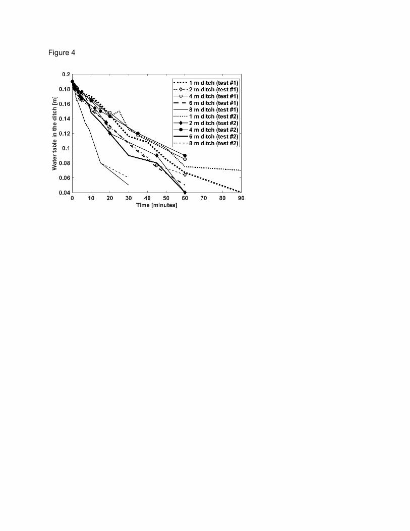
Figure 4

Figure 5

Figure 6

Figure 7
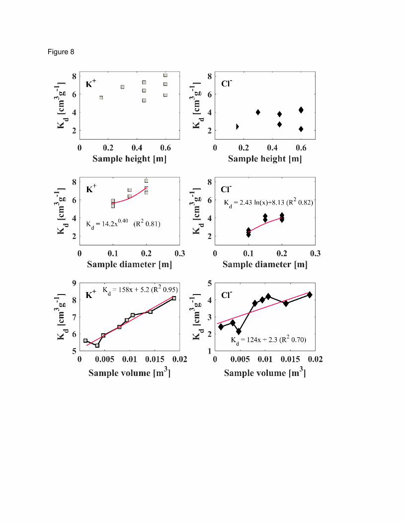
Figure 8

List of Tables
Table 1 Dimensions and number of undisturbed samples Table 2 Summary of the soil physical characteristics of 55 small-scale undisturbed soil samples Table 3 Basic statistics of K+ and Cl- dispersivity and partition coefficient derived from the 55 small-scale miscible displacements tests Table 4 Basic statistics of K+ dispersivity and partition coefficient derived from the large-scale miscible displacements tests Table 5 Basic statistics of Cl- dispersivity and partition coefficient obtained for the large-scale miscible displacements tests
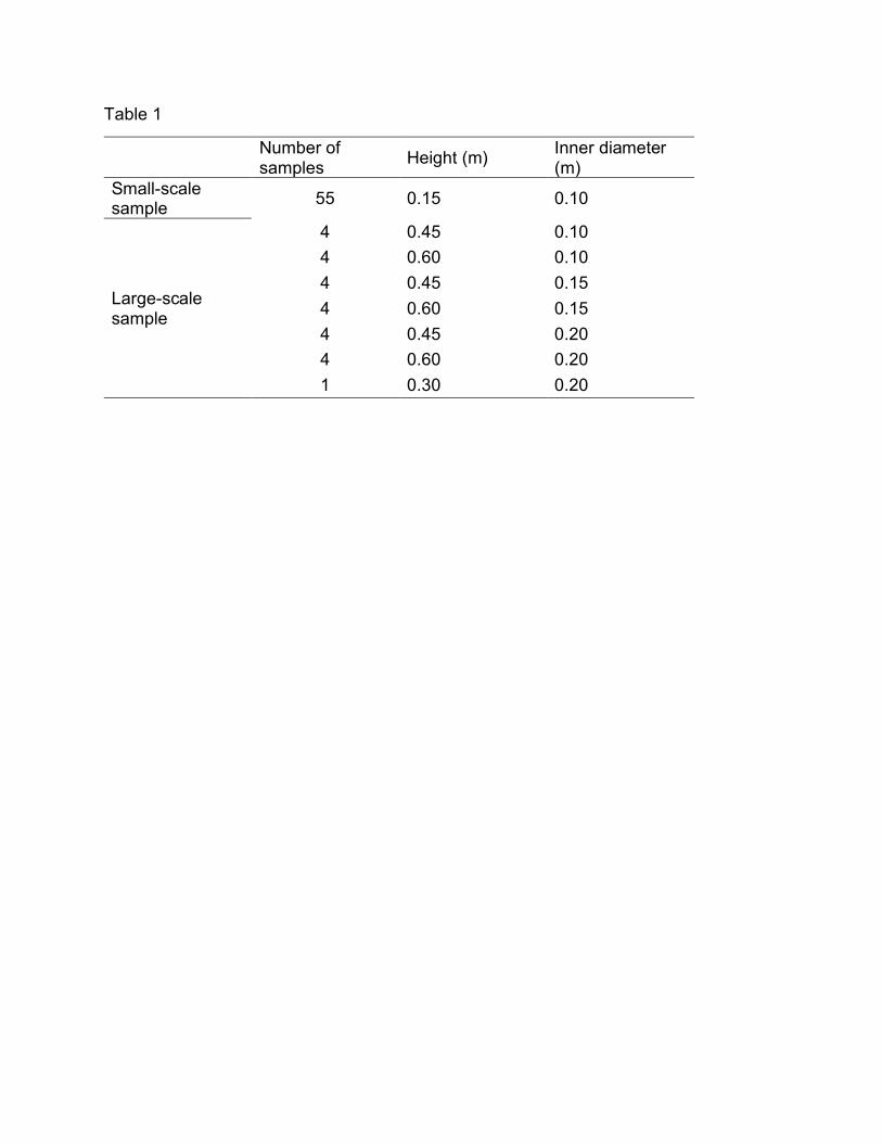
Table 1
Number of samples Height (m) Inner diameter
(m) Small-scale sample 55 0.15 0.10
Large-scale sample
4 0.45 0.10 4 0.60 0.10 4 0.45 0.15 4 0.60 0.15 4 0.45 0.20 4 0.60 0.20 1 0.30 0.20

Table 2
Property Mean SD CV Min Max n [ ] 0.51 0.04 0.08 0.42 0.58 ne [ ] 0.24 0.02 0.08 0.20 0.28 ρd [g cm-3] 1.34 0.10 0.07 1.14 1.59 CEC [cmolc Kg-1] 2.51 0.64 0.25 1.60 4.20 sand (%) 56.20 3.24 0.06 48.50 61.50 silt (%) 4.62 2.82 0.61 1.40 11.40 clay (%) 39.18 3.51 0.09 32.50 46.10 Ma [ ] 0.074 0.04 0.54 0.031 0.152 Mi [ ] 0.262 0.06 0.23 0.141 0.361 Me [ ] 0.172 0.05 0.29 0.099 0.263
SD: standard deviation, CV: coefficient of variation, Min: minimum value, Max: maximum value, ρd: bulk density, n: total porosity, ne: effective porosity Ma: macroporosity, Me: mesoporosity, Mi: microporosity, CEC: cation exchange capacity.

Table 3
Property Mean SD CV Min Max α [m] for K+ 0.18 0.19 1.05 0.003 1.50 α [m] for Cl- 0.10 0.08 0.75 0.002 0.34 Kd [cm3g-1] for K+ 1.71 2.27 1.33 0.040 16.7 Kd [cm3g-1] for Cl- 0.55 0.51 0.91 0.002 1.64
SD: standard deviation, CV: coefficient of variation, Min: minimum value, Max: maximum value

Table 4
Sample Name
Mean Maximum Minimum α [m] Kd [cm3g-1] α [m] Kd [cm3g-1] α [m] Kd [cm3g-1]
LC4510 0.409 1.60 0.52 1.95 0.32 1.23 LC6010 0.501 1.83 0.61 2.2 0.41 1.19 LC4515 0.394 2.01 0.57 2.6 0.36 1.34 LC6015 0.243 2.16 0.34 2.45 0.2 1.45 LC4520 0.545 2.28 0.65 2.91 0.47 1.67 LC6020 0.452 2.35 0.59 2.74 0.43 1.73 LC3020 0.606 2.65 0.76 2.98 0.44 2.33
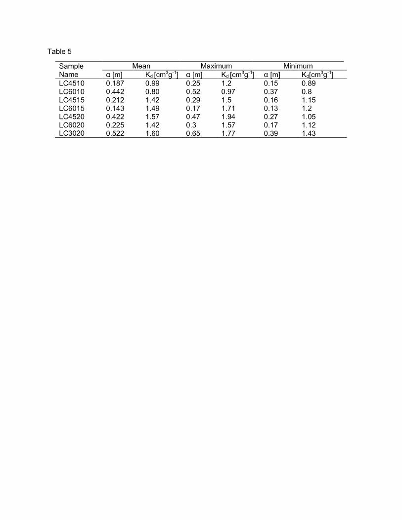
Table 5
Sample Name
Mean Maximum Minimum α [m] Kd [cm3g-1] α [m] Kd [cm3g-1] α [m] Kd[cm3g-1]
LC4510 0.187 0.99 0.25 1.2 0.15 0.89 LC6010 0.442 0.80 0.52 0.97 0.37 0.8 LC4515 0.212 1.42 0.29 1.5 0.16 1.15 LC6015 0.143 1.49 0.17 1.71 0.13 1.2 LC4520 0.422 1.57 0.47 1.94 0.27 1.05 LC6020 0.225 1.42 0.3 1.57 0.17 1.12 LC3020 0.522 1.60 0.65 1.77 0.39 1.43