BRANDEIS UNIVERSITY

Scalar Representation and

Inference for Natural

Language Senior Thesis

Michael Shafir

Advisor James Pustejovksy

Summer 2010 – Spring 2011

This work posits a computational framework for modeling the semantics of scalar expressions.

The framework builds off of a graph structure that stores relational knowledge between entities

as labeled edges, and derives new relationships through the transitive closures of the edge labels.

A categorial grammar composes the expressions into terms that actively construct the scalar

graph structure without the need for an intermediate level of logical representation. The vast

expressive capabilities of this system allow for a means of computationally applying current

theoretical research.

Shafir 2

Contents

Introduction ..................................................................................................................................... 4

Background ................................................................................................................................. 4

Approach ..................................................................................................................................... 8

Relational Scalar Modeling............................................................................................................. 9

Representation ........................................................................................................................... 10

A Relational Graph Model .................................................................................................... 10

Scalar Graph Computation .................................................................................................... 12

Comparison Classes ............................................................................................................... 14

Default Subclasses ................................................................................................................. 17

Formalizing the Graph ........................................................................................................... 19

Sample Representations ......................................................................................................... 21

Degree Modifiers ................................................................................................................... 22

Model Minimization .............................................................................................................. 24

Model Construction ................................................................................................................... 25

Compositionality and Categorial Grammar ........................................................................... 26

Type Ontology ....................................................................................................................... 28

Simple Predication ................................................................................................................. 28

Unification ............................................................................................................................. 31

Degree Modifiers ................................................................................................................... 33

Comparison of Averages ....................................................................................................... 35

Conjunction ........................................................................................................................... 36

Inference and Question Answering ........................................................................................... 37

Direct Relation Testing .......................................................................................................... 37

Set-based Question Answering .............................................................................................. 39

Further Development .................................................................................................................... 41

Negation .................................................................................................................................... 41

Quantitative Modeling............................................................................................................... 42

Shafir 3

Measurement Sensitivity ........................................................................................................... 44

Quantitative Adjustment and Classification .............................................................................. 44

Multidimensionality .................................................................................................................. 45

Scale Resolution and Lexical Semantics ................................................................................... 45

Conclusion .................................................................................................................................... 46

Bibliography ................................................................................................................................. 48

Shafir 4

1 Introduction Much of natural language conveys entity information valued along a continuum. Properties such

as weight, height, and size are scalar properties because their values are positions along the

continuums of those respective scales. A computational semantic system for natural language

must consider modeling and reasoning with such continuous values as well as discrete values in

order to truly capture the underlying information content. This work presents a set of techniques

for addressing some of the fundamental difficulties in building such a system.

It considers the following primary questions:

1. What informational content is inherent in scalar expressions?

2. How does one logically model or represent that information?

3. What information can be logically derived from scalar expressions?

The majority of the work will focus on these questions as they define the functionality of a scalar

reasoning system. The system will attempt to capture a small subset of possible expressions

exactly according to the proposed answers to these questions. Nevertheless, many of the core

approaches to these questions will be applicable to larger domain tasks.

This work discusses the construction of a computational semantic system akin to that of

Blackburn & Bos (2005). However, unlike Blackburn & Bos, this system will focus exclusively

on scalar knowledge. These works share a goal of simulating natural language knowledge with

rich semantic representation frameworks. These computational frameworks can better inform

research in theoretical semantics as well as other areas of computational linguistics.

1.1 Background

This section proposes a basis for the model-theoretic semantics that will be used to develop the

scalar representations of the underlying system. There has been a rich treatment of scalars in the

semantics literature, but most of this literature does not present computable solutions. I will

formalize a method of constructing a computable representation based from principles in the

literature.

In order to consider the process of constructing scalar representations compositionally from

utterances, one must carefully consider those elements of language that provide the scalar

knowledge. Though there are multiple ways to encode such knowledge in language, this work

will focus on the scalar information conveyed in gradable or degree adjectives.

As defined in Klein (1980), an adjective belongs to the class of degree adjectives iff:

i. It can occur in predicative position, i.e. after copular verbs

ii. It can be preceded by degree modifiers such as very

In addition, I present some fundamental assumptions about gradable adjectives that are

consistent with most other semantic analyses in the literature (Bartsch & Vennemann, 1973;

Shafir 5

Bierwisch, 1989; Cresswell, 1977; Heim, 1985, 2000; Hellan, 1981; Kennedy, 1999, 2001, 2007;

Kennedy and McNally, 2005; Klein 1991; Seuren 1973; von Stechow, 1984)

a) Gradable adjectives map their arguments onto abstract representations of

measurement or degrees.

b) A set of degrees ordered with respect to a common dimension, constitute a scale.

The above assumptions present a fundamental question of ordering. For a computational system,

one must ensure that the function will order the degrees without assuming additional

information. For example, assuming an ordering function functioning over degrees of height one

could expect the given ordering of the predications, short, average height, tall. However, what

underlying degrees would these predications map to?

One possible mapping would treat these predicates directly as the degrees. In this case, the

ordering function would simply order according to a strict master ordered list of all discrete

degrees in the appropriate dimension. For example, for height, the ordering function would order

its arguments according to their position in the list [short, average height, tall], assuming an

incremental height ordering. Given two degrees, let‟s say tall and short, it would order them by

their index in the master list thereby consistently producing the ordering [short, tall]. However,

such a system is not very extensible. One can imagine an endless scale of height degrees (very

tall, slightly short, very standard height). Furthermore, such a basis would prove impossible for

modeling quantitative data such as five feet tall. The degrees should be extensible and capable of

modeling quantitative data.

In an attempt to solve this issue, another possible mapping would assign contextually defined

numerical estimates to these gradable predicates. Bartsch & Venneman (1972) provide a norm

function to resolve this issue. The norm function they present takes a comparison class and a

property and returns the average degree of that property for the given class. Thus, tall would

compare as greater than the norm(people,tall), the norm function would return the average

height at which people are considered tall. When lacking specific numerical information for this

result, this function can be expressed as a variable over properties (Stanley 2000) or left

incomplete (Jacobson 2006). Crucially, there must be a way to continue with inference

computationally without providing or otherwise assuming this information. In addition,

Boguslawski (1975) presents a problem with the norm approach in that it imposes a direct cutoff

and by setting this average to be the average person, being above the average would not

necessarily imply the positive form (in this case tall). However, even though the numerical

average is not the appropriate factor for judging these classes, the idea of a cutoff threshold is

crucial in making a computational system.

In order to make this approach computable, we must wrap these norm functions as sets in the

underlying data. This can both solve the issue Boguslawski presents and allow us to delay the

assignment of numerical estimates. Consider again the semantics of tall, if we assume some

Shafir 6

threshold at which individuals are tall, there will be some exact value at which we can divide

entities into two sets (tall and not tall). The respective definitions would involve this threshold,

where is the threshold at which we make the split for that class. The following

definitions would thereby describe sets of tall people and not tall people:

However, Kamp (1975) disagrees with such a threshold. Given the task of classifying individuals

into the groups tall and not tall, there would likely be borderline cases which one could not

easily place into a single of the groups. Following Kamp, the two thresholds used would have to

have an interval between them. Klein (1980) proposes an alternate solution to classifying these

borderline cases by proposing a reapplication of the predicate tall on just the extension gap or the

borderline cases. For example, let us say that the threshold is computed by taking the average of

the individuals given to classify. Let‟s say that we can classify confidently only if the numerical

value is outside of half the standard deviation from the mean, then reapplying this operation on

just the unclassified instances (the borderline cases) will be able to classify more. After enough

successive iterations, all instances will be classified and the final threshold will be the concrete

value on which to split instances into the two classes. This roughly follows the concept of a soft

margin in an SVM classifier (See section 3.4).

Another issue remains with this approach. How would one formalize the notions of slightly tall

and very tall in comparison? It is evident that both would be subsets of tall and that certainly

there would be some interval that would be in neither subset. Again, some threshold would have

to distinguish between the classes. However, to maintain a compositional system, words such as

slightly must intelligently compose with the adjective they are used with. The semantics of these

degree modifiers, is quite complex. Consider, for example, the distinction between slightly tall,

slightly short, and slightly average. Slightly tall results in a higher mapping on the scale, slightly

short results in a lower mapping, and slightly average results in a less constricted range within

the average class. A successful system should automatically construct these meanings from the

composition of their parts.

Multiple semantic discussions of gradable adjectives cite the Sorites paradox as a problem in the

semantics of these expressions. An example of this paradox works as follows (given in Tye

1994):

1. There is a definite number, N, such that a man with N hairs on his head is bald and a man

with N+1 hairs on is head is not bald.

Intuitively negating the first principle yields the following assertion.

Shafir 7

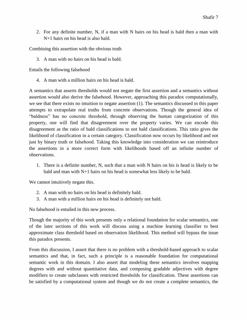
2. For any definite number, N, if a man with N hairs on his head is bald then a man with

N+1 hairs on his head is also bald.

Combining this assertion with the obvious truth

3. A man with no hairs on his head is bald.

Entails the following falsehood

4. A man with a million hairs on his head is bald.

A semantics that asserts thresholds would not negate the first assertion and a semantics without

assertion would also derive the falsehood. However, approaching this paradox computationally,

we see that there exists no intuition to negate assertion (1). The semantics discussed in this paper

attempts to extrapolate real truths from concrete observations. Though the general idea of

“baldness” has no concrete threshold, through observing the human categorization of this

property, one will find that disagreement over the property varies. We can encode this

disagreement as the ratio of bald classifications to not bald classifications. This ratio gives the

likelihood of classification in a certain category. Classification now occurs by likelihood and not

just by binary truth or falsehood. Taking this knowledge into consideration we can reintroduce

the assertions in a more correct form with likelihoods based off an infinite number of

observations.

1. There is a definite number, N, such that a man with N hairs on his is head is likely to be

bald and man with N+1 hairs on his head is somewhat less likely to be bald.

We cannot intuitively negate this.

2. A man with no hairs on his head is definitely bald.

3. A man with a million hairs on his head is definitely not bald.

No falsehood is entailed in this new process.

Though the majority of this work presents only a relational foundation for scalar semantics, one

of the later sections of this work will discuss using a machine learning classifier to best

approximate class threshold based on observation likelihood. This method will bypass the issue

this paradox presents.

From this discussion, I assert that there is no problem with a threshold-based approach to scalar

semantics and that, in fact, such a principle is a reasonable foundation for computational

semantic work in this domain. I also assert that modeling these semantics involves mapping

degrees with and without quantitative data, and composing gradable adjectives with degree

modifiers to create subclasses with restricted thresholds for classification. These assertions can

be satisfied by a computational system and though we do not create a complete semantics, the

Shafir 8

system proposed in this work can form a solid framework upon which one can construct a

complete semantics for scalar knowledge reasoning.

1.2 Approach

I propose several necessary elements for a successful and complete implementation of a degree

mapping semantics for gradable adjectives:

1. The semantics must be compatible with quantitative data.

2. In the absence of quantitative data, the system must still be capable of performing certain

inference. For example, very tall implies tall, tall implies above average height, but not

vice versa.

3. The set of possible degrees should be extendable without revision to the system. In other

words, the system should be capable of systematically enumerating all the possible

degrees for a certain dimension.

4. The semantics of degree modifiers should be fully compositional.

In addition to these elements, in order for the resulting system to be tractable, the model

constructed must be minimal and expand the available classes gracefully in order to

accommodate modeled data. For example, very tall people should not be a class initially, but

should be represented only when needed.

A Java implementation accompanies many of the principles laid forth. Through this

implementation one gains a perspective of the computational complexity of such tasks as well as

greater insight into difficulties that surround implementing a scalar reasoning system.

I begin by modeling only relational semantics. The implemented system will be only relational,

but it forms a foundation which can be extended with quantitative data as explained in the later

sections of this work. I first consider simple cases of relational predication and gradually expand

the domain of input. I follow the aforementioned principles from the literature on scalars, but my

approach presents many novel techniques necessary for a computational system of this type. The

semantics stem from necessity and the only requirement is that the modeled data be consistent

with human intuition.

In order to feasibly construct this system, I must restrict its domain. Throughout this work a

number of issues will remain unresolved thereby allowing us to focus acutely on the task at hand.

The models constructed here will be exclusively static and ignore dynamic temporal, aspectual,

or modal information. Many of the algorithms will be brute force and thereby, computationally

inefficient for the purpose of greater depth of research. The logical reasoning will focus only on

theorem proving relevant to the immediate task, and discussions of other logical reasoning

alternatives will remain outside the scope of this work. The work will also ignore issues of

ambiguity, where not directly relevant to scalar reasoning.

Shafir 9

This work first discusses the modeling of information. How can we capture the scalar

information content contained in natural language utterances? I propose a relational graph data

structure and provide the algorithms that handle relation insertion and retrieval, along with other

crucial tasks such as minimization.

Following representation, I will discuss the semantics that construct those representations. This

section will focus on assigning compositional semantic expressions to the items in the lexicon

and ensuring that different possible combinations of expressions create the correct target

representation.

The final relational modeling section discusses the compositional semantics for retrieving

information from the representation via question answering.

The final section of the work presents numerous possible extensions to the existing framework.

These extensions require further research, but nevertheless, can extend from the provided

implementation. The implementation that accompanies this work provides an open framework

upon which many principles of scalar modeling and reasoning can be applied.

I hope that by discussing a system based upon the points above, I can present a foundation for

reconsidering these theories and reevaluating such semantic discussion in terms of its

computability.

2 Relational Scalar Modeling

In order to focus on capturing the compositional semantics, I will ignore issues of quantitative

data for the moment and will return to these issues in a section 3.

This section will propose a system of representing relational scalar data and a model theoretic

semantics for constructing those representations. By relational scalar data, I refer to data that

compares two entities or classes along a dimension.

Consider a set of utterances appropriate to capture with such a system:

1. John is taller than Bill.

2. John is tall.

3. Bill is a tall person.

4. Sam is very tall.

First, I consider what an appropriate representation of such knowledge should be, and describe a

graph structure capable of storing this knowledge. Then, I construct a compositional system

capable of building those representations. Finally, I propose a model-based logic for checking if

new information is informative and consistent with a given model, and develop a system of

information retrieval via natural language queries.

Shafir 10

2.1 Representation

2.1.1 A Relational Graph Model

Consider the informational content given in a comparison such as (1) above. By saying John is

taller than Bill we are assigning a greater than relationship to the two on the scale of height. The

exact mapping of the heights on the height dimension is unnecessary. We can represent this as

.

5. John is shorter than Mary.

Adding sentence (5) introduces a new relationship into the model: .

Importantly, a new entailment can arise from this information considering (1):

. Deriving this relation involves applying transitive closure rules to the given

relationships. One such closure rule would be given as follows:

We can fully capture the information and entailments for these expressions under a model that

stores these direct relationships and derives new ones. However, this approach would not be the

only solution as we shall see. Take, for example, the following set of greater than relationships

on an arbitrary unspecified scale.

Now, imagine an algorithm to test if . It could search for all relationships that have as

greater than another entity, for each one it finds, it will search for all relationships with the right-

hand entity as greater than, and continue like before. If it finds a at any point, then this

relationship holds. Essentially, the previously described algorithm is a depth-first search across

relationships connecting them by the closure rule given above. Thus, our model would

essentially be a graph and retrieving relationships would be akin to traversing the graph. We can

reconstruct (6-9) in a graph data structure visualized with directed arrows representing a greater

than relationship.

Shafir 11

Figure 2.1.1-1

Using the graph data structure represented above, we would merely need to start at and attempt

to find a path to . At worst case, provided that the graph is acyclic, the complexity of this path

finding operation would be O(E) where e is the number of edges in the graph. While storing the

knowledge of (6-9) in a hash table could also have similar complexity, the graph representation

approaches the problem at hand more directly.

2.1.1.1 Transitive Closure

In order for such operations to work, we must define a core set of relationships and provide the

complete set of closure rules over that set. The following table presents the baseline set of

relationships that we will build off of, and the convention by which they will be notated in this

work.

Relationship Notation Visualization

Equal

Not Equal

Greater Than

Less Than

Greater Than or

Equal To

Less Than or

Equal To

Relationship is

unknown

Table 2.1.1-1

Shafir 12

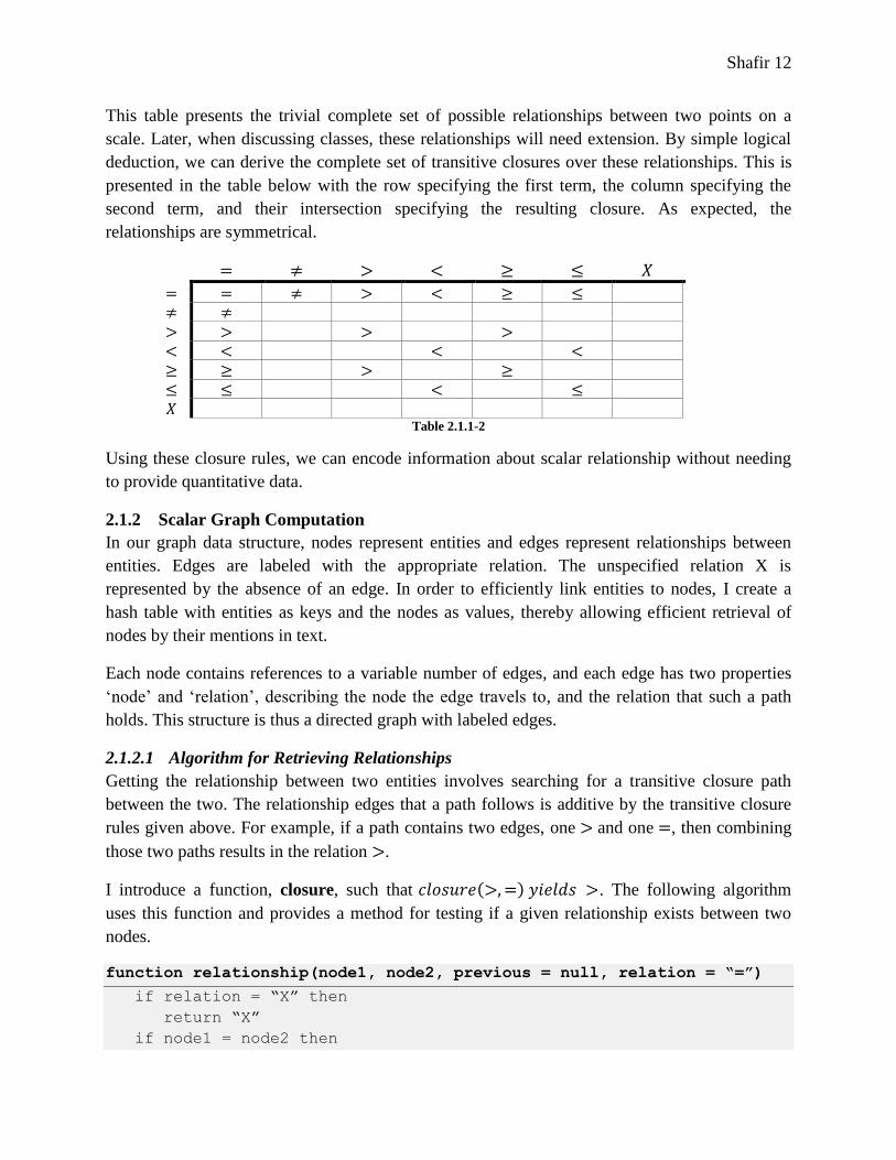
This table presents the trivial complete set of possible relationships between two points on a

scale. Later, when discussing classes, these relationships will need extension. By simple logical

deduction, we can derive the complete set of transitive closures over these relationships. This is

presented in the table below with the row specifying the first term, the column specifying the

second term, and their intersection specifying the resulting closure. As expected, the

relationships are symmetrical.

Table 2.1.1-2

Using these closure rules, we can encode information about scalar relationship without needing

to provide quantitative data.

2.1.2 Scalar Graph Computation

In our graph data structure, nodes represent entities and edges represent relationships between

entities. Edges are labeled with the appropriate relation. The unspecified relation X is

represented by the absence of an edge. In order to efficiently link entities to nodes, I create a

hash table with entities as keys and the nodes as values, thereby allowing efficient retrieval of

nodes by their mentions in text.

Each node contains references to a variable number of edges, and each edge has two properties

„node‟ and „relation‟, describing the node the edge travels to, and the relation that such a path

holds. This structure is thus a directed graph with labeled edges.

2.1.2.1 Algorithm for Retrieving Relationships

Getting the relationship between two entities involves searching for a transitive closure path

between the two. The relationship edges that a path follows is additive by the transitive closure

rules given above. For example, if a path contains two edges, one and one , then combining

those two paths results in the relation .

I introduce a function, closure, such that . The following algorithm

uses this function and provides a method for testing if a given relationship exists between two

nodes.

function relationship(node1, node2, previous = null, relation = “=”)

if relation = “X” then

return “X”

if node1 = node2 then

Shafir 13

return relation

for all edges e from node1

if e.node <> previous then

new_relation <- closure(relation,e.relation)

result <- relationship(e.node, node2, node1, new_relation)

if result <> “X” then

return result

return “X”

Essentially, this algorithm recursively traverses the graph depth-first while tracking the previous

node to prevent back-tracking. It traverses until closure rules result in an unknown relationship

(X) or until the target node is found. I present it here as a recursive depth-first algorithm for

clarity of presentation, there is no theoretical motivation for this approach. It is crucial to note

that such traversal algorithms require the graph to be acyclic. This property must be maintained

across all modifications to the graph structure.

2.1.2.2 Algorithm for Inserting Entity Relationships

The model cannot contain all entities and possible relationships at the start, but rather must be

minimal and expand to include new entities and relationships when they are mentioned. We link

entities to nodes by a hash map (node_map in the pseudocode). The insertion algorithm

crucially avoids creating a cycle by only adding an edge where no previous relationship existed

(disconnected nodes).

function add_relation(entity1,entity2,relation)

node_added <- false

if entity1 not in node_map then

node_map[entity1] <- new node(entity1)

node_added <- true

if entity2 not in node_map then

node_map[entity2] <- new node(entity2)

node_added <- true

node1 = node_map[entity1]

node2 = node_map[entity2]

if not node_added then

current_relation = relationship(node1,node2)

if current_relation = relation then

return “Not informative”

else if current_relation <> “X” then

return “Not consistent”

node1.edges.add(edge to node2 labeled relation)

node2.edges.add(edge to node1 labeled symmetrical(relation))

Here we add the entities to the model if they do not exist, but if they both exist then we check

what the current relation is to ensure we are not inserting redundant or inconsistent data. If these

Shafir 14

conditions pass then we insert the appropriate edge (bidirectional so that we allow future graph

traversing to go both ways). The function symmetrical returns the symmetrical reverse of a

relation. This is done by lookup. The symmetrical relationships to and are and

respectively, and vice-versa. All other relations are their own symmetrical counterpart.

By storing symmetrical relationships immediately, the system can capture entailments such as

(6) below.

5. John is taller than Mary. Mary is shorter than John.

2.1.3 Comparison Classes

Modeling scalar relationships may seem relatively straightforward when considering the cases

above, but, the above formalisms fail to capture the modeling of comparison classes and how

they would fit into a scalar representation. I will extend the current formalism to allow for

entailments based off of comparison classes:

6. Elephants are taller than mice. Dumbo is a short elephant. Mickey is a tall mouse.

Dumbo is taller than Mickey.

7. Men are taller than women. John is a tall man. Mary is a short woman. John is taller

than Mary.

8. John is a tall person. Bill is a short person. John is taller than Bill.

While proposing structures to incorporate such reasoning, it is crucial to maintain a minimal

model and delay modeling class relationships until absolutely necessary or else then entire

ontology would be present in the model from the start.

The first required modification to the system would be to allow the representation of classes as

currently, our model only stores information about individuals. From examples (7) and (8)

above, it is evident that classes participate in similar relationships to individuals, so it would be

appropriate to model them similarly.

Let us first consider example (7). We have a class of elephants and a class of mice and we

introduce a greater than relationship between the two such that any member of the elephant class

would be greater than any member of the mouse class. In addition to adding classes into our

model, this logic requires the addition of member relationships and rules over those new

relationships. We propose the following new relationships:

Relationship Notation Visualization

Contains

Member of/

Contained by

Table 2.1.3-1

Shafir 15

A set of rules follow implicitly from these new relationships, with R being any relationship

except the two above.

1.

2.

3.

The first two rules are trivial, but the third rule requires some explanation. It is through this rule

that the entailment in (7) will follow: if elephants are taller than mice and Dumbo is an elephant,

then Dumbo is also taller than mice. Put simply, relationships on the class apply to the members.

However, this rule cannot be expressed as a transitive closure rule, and thus, cannot currently be

incorporated into the model without a modification to the earlier system and algorithms. It does

not fit with the earlier closure rules because it is not symmetrical and it is ordered:

but and . While we can express these restrictions

in the closure function, there still exists a limitation in the tree traversal algorithm in that the

results will not be symmetrical. Consider the following example.

Figure 2.1.3-1

With the described closure modification, traversing the graph from a to d results in the

relationship “>”, but traversal from d to a will stop at c because there does not exist a closure

rule for the relationship. Furthermore, none of the previously defined relations properly

capture the relationship between b and d and vice versa. Nonetheless, the relationship between

these two nodes is slightly more informed than “X”. Since b is a class and d is a class or an

entity in this case, and classes express a range of values, a different set of relations apply here.

Given that a class has thresholds at its limit and not instances, the range of a class on a scale does

not include the thresholds, but rather the values between them. Consider the following

representation of a class range:

Class Table 2.1.3-2

There exist a number of possible relationships to this class. The table below shows all the

possibilities of ranges in which we can model the values of individuals or the ranges of other

classes.

Shafir 16

Greater than

Less than

Inclusive greater than

Inclusive less than

Equivalent

Not Equivalent

No Relation Table 2.1.3-3

The above chart is by no means complete as there are certainly additional relationships, such as

partly inclusive relationships, that exist. However, when we consider what these relationships

describe about the members of the classes being related, we see that such additional distinctions

are unnecessary. For instance, if class A is greater than class B, then all elements of class A are

greater than all elements of class B. If class A is inclusively greater than class B, this says

nothing about the relationship between the elements in the two classes since class B can be

greater than, less than, or equal to any of the elements in class A at that time. Since this

collection of members can change at any point, anything more specific than this open

relationship will be more difficult to maintain. We give only the relationships that store relational

information that is constant with respect to insertions and deletions.

What does the inclusive greater than relationship specify if it makes no claim about the elements

of two classes? It is in combination other relationships that it becomes useful. For example, if

class A is inclusively less than class B, then anything greater than all of class A is also greater

than all of class B. Through this, we can provide new transitive closure rules that will allow for

bidirectional traversal of a relational graph with membership relations. We extend our closure

table with cross-class relationships. Notice that many of the cross-class relationships are

equivalent to the individual relationships. This is because the ranged operators subsume the logic

of the individual operators.

We exclude containment relationships from this discussion because such relationships do not

help in achieving the target entailments. In fact, such relations are difficult to express in natural

language.

The following chart represents the revised set of closure relationships.

Shafir 17

* *

*

* Table 2.1.3-4: * - these are additional containment relationships, which are excluded from this discussion

By modifying the closure function with the relationships above, we can capture the new

relationships without much modification to the algorithms previously proposed. Returning to our

target example, we can model the given relationships as follows.

Figure 2.1.3-2

Traversing from Dumbo to Mickey gives the relation sequence , which yields as the

closure, while the reverse, , yields as the closure. These are the correct entailed

relationships.

In order to adjust our system to the new transitive closure rules, we must make a slight

modification to the algorithms that retrieve node relations. The relationship begins its transitive

closure sequence with the relation „=‟. However, since equality does not have a transitive closure

with membership or containment, this algorithm will no longer be able to retrieve these

relationships. Instead, if we create a new relation for an exact match and add that this relation‟s

transitive closure with any other relation returns that other relation, then this issue will be

resolved.

There exist additional possible relationships between classes that are left unexplored by this

discussion. Such relationships introduce complex factors outside the scope of this work. These

relationships are not inconsistent with the observations and algorithms put forth here, but rather

require additional information that relies on quantitative metrics. The above relationships are

sufficient for the purposes of this work.

2.1.4 Default Subclasses

However, the relationship does not fully model the fact that Dumbo is a short elephant. We must

incorporate the semantics of short, average, and tall into our model. From an earlier discussion,

Shafir 18

it is clear that all three are contained subclasses with thresholds specifying their boundaries.

These subclasses exist for any modeled class and have a constant ordering. We can model these

subclasses within the class people as follows.

Figure 2.1.4-1

It is evident that this approach without extension does not support quantitative data, but we will

provide the methodology to add this in a later section. For the purposes here, it is adequate.

Furthermore, these three subclasses alone are not enough to capture Consider example (10).

9. John is above average height. John is tall.

Being of above average height does not entail being in the subclass tall. Boguslawski (1975)

targeted this principle as an argument against gradable adjectives mapping their arguments onto

degrees in relation to an explicit average. However, no single norm function can allow this

distinction. In modeling the semantics of these expressions one must capture exactly the

information the data provides, as there is no generalization that will capture the information in

(10). Above average height and tall are both subclasses of individuals with exact relationships to

the average of their class. To model the distinction, we can say that tall is a subclass of above

average height. Yet, the distinction between these two classes is not always clear. In fact, the use

of above average can refer very different ranges across different scales. For example, above

average intelligence could certainly entail the predicate smart, where for a scale such as height

this is much less likely. In considering the default subclasses for the model, it is important to

allow just those categories which are necessary for representation to keep the model minimal and

ensure it properly explains the subclassing phenomena.

In order to determine this minimum, it is important to formalize the system by which new

subclasses are created. To do this, we must consider which elements of the semantic content of

each predicate that can be made atomic. For example, tall refers to a class greater than the

average class, while average height refers to a class of individuals within a certain range

including the numerical average of the superclass. By this description, we can reduce average

height to be constructed as a class with a contains relationship to the numerical average for its

superclass. Similarly, tall can be constructed as a class greater than the average class. By storing

these relationships, we can determine how to create these subclasses when they are needed, and

retain a minimal model otherwise.

Shafir 19

2.1.5 Formalizing the Graph

From this discussion we can formalize the concept of a node in the relational graph and what it

can capture. A node can represent the following:

1. The relative placement of an individual within a scale (graph).

2. The relative placement of the range of possible values for a class within a scale

(graph).

3. An anchor representing the average for its parent class.

The third category stems directly from the primitives of the previous section. Each of the

subclasses discussed related to an anchor to the average for a class. This anchor is crucial to

interpreting those subclasses relative to each other.

This anchor is a special case in the graph structure. Though it relates to the class it anchors, we

do not want inference to return it as a member. It should not participate in the same membership

transitive relationships as other contained nodes. Therefore, I define two additional relationships

that do not participate in the transitive closure rules from before. Avg is the relationship from the

class to its average anchor, and Avg-of is the reverse relationship from the average to the class it

anchors.

Despite these different nodes, the expressive capability of the system is not hindered by the fact

that nodes can represent both individuals and classes. We need not distinguish between them in

the algorithms because the relations relate both individuals and classes so that the transitive

closure rules follow equivalently regardless of whether the node represents a class or an

individual.

We identify each node of the graph uniquely by its base class or individual name and an ordered

set of relationships from that base. The following cases exemplify this.

John – ID[ John, { } ]

people – ID[ people, { } ]

average sized people – ID[ people, {avg-of, contains} ]

tall people – ID[ people,{avg-of, contains, greater-than} ]

When adding a relationship with a node that does not yet exist, we modify the algorithms to

create these derived classes and use the new IDs instead of just entity name. If the base class

does not yet exist, we create it. Then, we expand creating nodes for an expanding subset of the

relation set if they do not yet exist. The following algorithm retrieves a node from the graph or

creates it if it does not exist, adding the relationships as discussed.

function retrieve_node(id)

if id not in node_map then

if id.set = null then

node_map[id] = new node(id) //create and add the node

Shafir 20

else

//create and add the node

this_node <- new node(id)

node_map[id] <- this_node

//get the previous node

subset <- id.set[0:-1] //all elements except the last

prev_id <- new ID(id.base,subset)

prev_node <- retrieve_node(prev_id)

//get the relation to the previous node

relation <- id.set[-1] //the final element

//add the new relationship

this_node.edges.add(prev_node, relation)

prev_node.edges.add(this_node, symmetrical(relation))

return node_map[id]

This function is nearly complete, but it fails to store some crucial information. The class “tall

people” must not only relate to the class “average people”, but must also relate to the average

and the overall class. Each id with a larger set must maintain some relationships of the earlier

sets. Since we take avg-of to be a special case of member-of, then to all non-average nodes, we

translate avg-of to member-of. Consider the following example.

tall people – ID[ people,{avg-of, contains, greater-than} ]

o relations: greater than the class of average height people , member of people

class

Notice that “contains average height” is not a legitimate relationship. This is because it is

inconsistent with the first relationship.

We can store these additional relationships by taking subsets of the ID and adding relationships

when there is no inconsistency formed. We perform the following algorithm in place of adding a

new relationship in retrieve_node. It will add the required relationship and all of the derived

ones.

function add_derived_relationships(id,subset)

if length(subset) = 0 then

return

relation <- subset[-1]

if relation = “avg-of” then

relation = “contained-by”

node1 <- node_map[id]

node2 <- node_map[new ID(id.base,subset[0:-1])]

if consistent(relation,relationship(node1,node2)) then

node1.edges.add(node2, relation)

node2.edges.add(node1, symmetrical(relation))

Shafir 21

add_derived_relationships(id,subset[0:-1])

The only consistent relationships are or with and any relation with the unknown relation.

Greater than or equal to and less than or equal to only exist as a result of transitive closure and

are never inserted directly into the graph and member-of is a special case of those relations.

In addition, any time a new node gets added to the graph, we must ensure that the system will

search for parent classes and child entities or subclasses of that node. Such a process occurs in

the implementation after derived relationships have been added.

2.1.6 Sample Representations

Now that we have described a system capable of modeling our original examples, we will revisit

them.

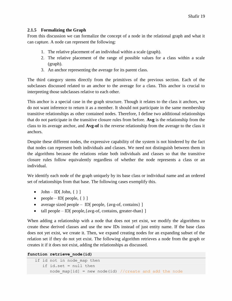
7. Elephants are taller than mice. Dumbo is a short elephant. Mickey is a tall mouse.

Dumbo is taller than Mickey.

This representation models the classes of elephants and mice as well as the average anchors and

average, tall, and short subclasses.

Figure 2.1.6-1

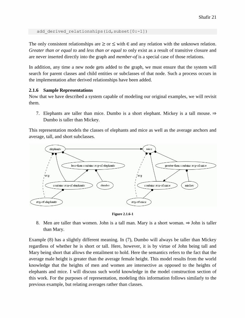
8. Men are taller than women. John is a tall man. Mary is a short woman. John is taller

than Mary.

Example (8) has a slightly different meaning. In (7), Dumbo will always be taller than Mickey

regardless of whether he is short or tall. Here, however, it is by virtue of John being tall and

Mary being short that allows the entailment to hold. Here the semantics refers to the fact that the

average male height is greater than the average female height. This model results from the world

knowledge that the heights of men and women are intersective as opposed to the heights of

elephants and mice. I will discuss such world knowledge in the model construction section of

this work. For the purposes of representation, modeling this information follows similarly to the

previous example, but relating averages rather than classes.

Shafir 22

Figure 2.1.6-2

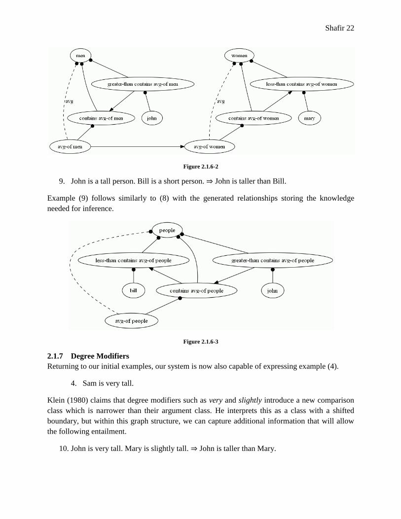
9. John is a tall person. Bill is a short person. John is taller than Bill.

Example (9) follows similarly to (8) with the generated relationships storing the knowledge

needed for inference.

Figure 2.1.6-3

2.1.7 Degree Modifiers

Returning to our initial examples, our system is now also capable of expressing example (4).

4. Sam is very tall.

Klein (1980) claims that degree modifiers such as very and slightly introduce a new comparison

class which is narrower than their argument class. He interprets this as a class with a shifted

boundary, but within this graph structure, we can capture additional information that will allow

the following entailment.

10. John is very tall. Mary is slightly tall. John is taller than Mary.

Shafir 23

Essentially, if we split the class of tall people into three categories like before (slightly, average,

and very), we see that the same mechanism that exists for class extension exists again here. We

will need an additional average anchor to the tall class and we can construct additional nodes

from that. Let us look at the resulting node for the “tall people” class and how it relates to the

“very tall people” and “slightly tall people” subclasses.

tall people – ID[ people,{avg-of, contains, greater-than} ]

very tall people – ID[ people,{avg-of, contains, greater-than, avg-of, contains, greater-

than } ]

slightly tall people – ID[ people,{avg-of, contains, greater-than, avg-of, contains, less-

than } ]

We note from this that “very” doubles the relation set of its argument and “slightly” doubles the

relation set and inverts the final relation. This transformation holds identically with the “short

people” class.

short people – ID[ people,{avg-of, contains, less-than} ]

very short people – ID[ people,{avg-of, contains, greater-than, avg-of, contains, less-than

} ]

slightly short people – ID[ people,{avg-of, contains, greater-than, avg-of, contains,

greater-than }

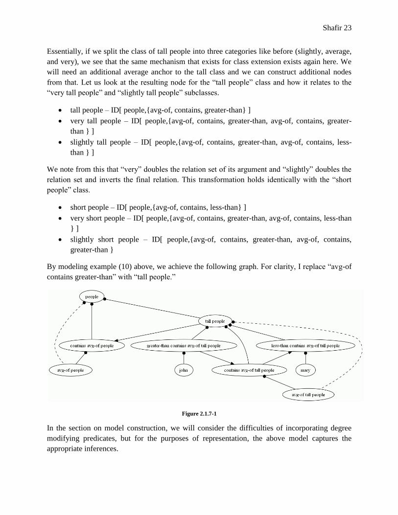
By modeling example (10) above, we achieve the following graph. For clarity, I replace “avg-of

contains greater-than” with “tall people.”

Figure 2.1.7-1

In the section on model construction, we will consider the difficulties of incorporating degree

modifying predicates, but for the purposes of representation, the above model captures the

appropriate inferences.

Shafir 24

2.1.8 Model Minimization

Though the current system captures the intended information, adding containment relationships

allows for redundancy. Essentially, if we model specific information before more general

information, then we introduce redundant edges into the graph. Take, for example, the following

chain of input.

10. John is taller than Mary.

11. John is a tall person. Mary is a short person.

Modeling (11) first and then (12) results in the following model.

Figure 2.1.8-1

The edge between John and Mary is a redundant edge that was originally informative by

statement (11). Removing this edge requires a minimization procedure to look for multiple paths

between any two given nodes. Since the bisymmetrical relationships, equality and inequality, do

not have transitive closure rules over the membership relations, they will never become

redundant, which is crucial because such redundancies would introduce cycles into the

representational graph. Having cycles in the graph will break the current system.

The issue at hand is instead one of acyclic redundancy. These redundancies do not affect the

proper operation of the algorithms presented earlier and therefore, one possible solution would

be to ignore such redundancies.

However, such redundancies do inhibit future systems where such edges can be given

quantifiable values. Having redundant edges in these scenarios adds an additional maintenance

overhead that may greatly reduce the efficiency of the system. In other words, if edges had

additional attributes attached to them, then keeping redundant edges will require the

synchronization of those attributes. For this reason, it is important to provide a means of

removing such redundancies.

A basic minimization algorithm would find all the paths from one node to another and would

remove all paths but the longest (most general) by removing single edge paths where multiple

Shafir 25

edge paths exist. Performing such an algorithm for every pair of nodes would result in a

complexity of . There are many adjustments that could reduce the complexity, but for the

purposes of this overview, this basic algorithm will suffice.

function minimize(graph)

for each node n1 in graph

for each node n2 in graph

paths <- breadth first search to find all paths from n1 to n2

longest <- path in paths with longest length

for each path p in paths

if p < longest and size(p) = 1 then

remove edge p[0] from graph

The minimization algorithm will encounter an error with one issue of the graph structure that has

not yet been resolved. Minimization and the relationship retrieval algorithm both assume that

there is only one possible relationship between two nodes. However, not all relationships are

exclusive. A node can be both inclusively greater than and contained by another node. Consider,

for example, the relationship of the node “tall people” to its parent class “people” as one such

relationship. In these cases, the containment relationship is more informative and another form of

redundancy exists. We are not storing this redundancy, but we must ensure that such dual

relationships always result in containment when retrieving relationship, and don‟t conflict with

minimization.

To remedy the retrieval issue, we modify the algorithm to recursively find all paths and return

containment where there is the ambiguity. In minimization, we never want to remove

containment edges in these cases, and since containment is always a single edge for every two

edges in an inclusive path, it will be the target of removal, preventing the retrieval of these

inclusive relationships prevents this problem.

Without these redundancies, our model will be minimal and we have shown it to be capable of

capturing direct relationships and more general class relationships involving subclassing and

degree modifiers. Now that we can represent such statements, we must develop the system which

will build these representations from natural language.

2.2 Model Construction

The process of model construction is essentially the process of converting natural language

sentences into functions that, upon execution, create the desired representation. Words, or even

morphemes, must contribute to this function. In order to allow this contribution to occur, these

functional contributions must be combined in a systematic way. The task is one of functional

programming and the principle of combining word “meaning” follows from Montague‟s notion

of compositionality. In this section, we will lay out the compositional process that will construct

the graph representations described previously.

Shafir 26

2.2.1 Compositionality and Categorial Grammar

We arrive at compositionality out of computational necessity. By considering the functional

meaning of words and how those functions combine, we not only more clearly understand the

underlying linguistic phenomena, but create a useful abstraction that splits the task of

construction into multiple subtasks dictated by word meaning. However, our use of

compositionality will differ from the formal semantic literature to focus on the computational

challenges of this particular problem.

In order to compose the functions, we must parse the sentences into a structure that properly

attaches arguments to the function. A categorial grammar will achieve this exact purpose. We

implement a categorial grammar by giving each lexical item a context in which it composes.

When it occurs in that context, we pass its function the arguments of the context in the proper

order. We encode our lexical items in an XML markup schema specifically designed for this

purpose. The schema specifies any contexts in which a specific lexical item occurs. Each context

consists of a lambda function for that word and an ordered set of its environment, labeled by

variables to be bound by the function. The type of the environment must be specified along with

the result type for the expression. Though the result can be inferred, building such inference is

outside the scope of this work. A sample markup for the copula “is” demonstrates several

contexts below.

Contexts for „is‟

<Context Function="(b a)" ResultType="t">

<ContextVariable Label="a" Type="noun"/>

<ContextVariable Label="this"/>

<ContextVariable Label="b" Type="adj"/>

</Context>

<Context Function="(unify a b)" ResultType="t">

<ContextVariable Label="a" Type="noun"/>

<ContextVariable Label="this"/>

<ContextVariable Label="b" Type="noun"/>

</Context>

Notice the variable “this” indicates the position of the head word relative to its arguments.

These entries define the categorial grammar and provide the necessary information for

composition to occur. However, a challenge still lies in parsing natural language input with this

grammar, and there are multiple algorithms through which this can be achieved. We take the

simplest and least efficient approach in this process because it is not the focus of this work. To

get all possible parses, we implement a brute force, non-deterministic, shift-reduce parser. It

works efficiently enough for the purposes here. Expressions are combined if a context matches

around a head word. At the end, any resulting functions of type “t” are returned. Simplifying and

evaluating these functions on a model results in the required transformation on that model.

Shafir 27

The functional language used in specifying the meanings of the lexical items must be expressive

enough to create the required representations. As I discuss this process, I will introduce new

primitives into the language as they are needed. Throughout the remainder of this section, I will

notate these functions as expressions in the lambda calculus and ignore issues of argument

ordering by the assumption that they are resolved by the categorial grammar and can be

intuitively resolved by the reader.

The expressions will be implemented within Java in an expression library built for this purpose.

The library follows the evaluation procedure of lambda calculus, which we will define

recursively.

Formally we define the grammar as follows:

We give the grammar for types and the grammar for expressions. For types, Greek letters

represent the constant base types. For expressions, c stands for the primitive expressions and

constants that we will design and x represents variables. Terms satisfying the above grammar are

not necessarily valid terms in this language. Testing validity requires type checking to ensure

that the types of the expressions are compatible. However, the process of checking expression

validity is not necessary for this task. Instead, we will simplify expressions according to the

following rules and if the result is a single primitive call (a constant function with constant

arguments), then we proceed to evaluation, otherwise we throw an error.

The process of application is identical to that of the type-free lambda calculus. It is a substitution

operation where the argument replaces the variable occurrences, with variables first renamed so

the argument and head term do not conflict. We follow the Church system of simply typed

lambda calculus in which the argument types are explicit. For a formal introduction, see

Barendregt & Barendsen (2000).

Shafir 28

We will implement this system and build off of it as a basis for semantic composition.

2.2.2 Type Ontology

Much of the discussion on representation has dealt with the modeling of class relationships.

However, we have yet to formalize the means by which such class information will be available

to the expressions. In order to provide this information, we will need a type ontology, and in

order to integrate this ontology with the expressions, we must type them according to the

ontological types and not just syntactic types. The goal here is not to create a full ontology, but a

minimal ontology that provides the necessary information to model class relationships. The

grammar will be sensitive to the types in this ontology. I will encode them in the XML Markup

by allowing each item to specify its parent types. I allow for multiple types to avoid limiting the

expressivity of the system since multiple inheritance is common in natural language.

The ontology will be specified by the lexical items and their relationships, and the grammar will

allow context matching based on supertypes in the resulting type hierarchy. The notion of a type

hierarchy is compatible with our typing rules and requires only one additional rule.

These types are specified in a base lexicon of the lexical items. The lexicon provides the

contexts, functions, types, and any additional information about the items. The items in lexicon

provide information that is constant across models. In addition to the base lexicon, the model

will have its own lexicon linking to items in the base. The model‟s lexicon will have instance

items and model knowledge that are variable across models. The parsing system will use both

lexicons to construct expressions. The model‟s lexicon will provide objects for the expressions to

use and the base lexicon will provide all other subexpressions.

2.2.3 Simple Predication

Now that I have established our grammar and semantic composition system I can begin

analyzing the semantics of the natural language input to our system and how the semantics

combine. I begin with simpler sentences and expand to cover more advanced cases. The first

case I cover is adjectival predication.

1. John is tall.

To inform the compositional process, we must first decide upon the proper final interpretation of

this sentence. In reality, the interpretation is quite complex since it must infer type comparison

class of John, knowledge that may be presupposed or previously known. Since this system does

not deal with presupposition, we will assume that the system already knows that John is of the

class “people.” With this assumption, example (1) must create the following representation in the

scalar graph of the height dimension.

Shafir 29

Figure 2.2.3-1

Remember that upon retrieval of a node with ID [people, {avg,contains,greater}], the

representation system will create the relevant nodes and relationships between them. Essentially,

only a single call of the algorithm add_relation is necessary for creating this model.

However, this operation must be performed on the scalar graph for height, thereby introducing

the question of how graphs along different dimensions will be managed.

To resolve this question, I create a function for the overall model that adds relations into specific

graphs. This function takes the same arguments as the add_relation function on the scalar graph

with an additional dimension argument. We store graphs in a hash table by dimension and if the

dimension does not yet exist, we insert an empty graph into the hash table for that dimension. To

the model, I represent the added information content of example (1) in the following shorthand.

This represents calling the add_relation function on the model with the arguments described

above.

To link the functions of the model with expressions in the compositional system, we provide

them as primitive functions to be evaluated after the expressions are simplified. In the

information, add_relation is a primitive function, john and people are objects (a primitive type

denoted by brackets) drawn from the model and lexicon respectively, “height” is a primitive

string, relations (such as and ) are primitives, and is a primitive relation set

constructed from relations. Since we need to reference nodes, I introduce a second primitive

function node, which takes a base node and relation set and creates the appropriate node ID.

Finally, since the natural language input does not have the class people, we must provide a way

of attaining it by retrieving the type of john. A third primitive function, typeof will do this by

returning the first immediate supertype of an object. These primitives will suffice for providing a

basic semantics for example (1).

Shafir 30

Considering constituency, john is the final word to compose, so abstracting it out of the above

function we get:

Taking this as the semantics of “is tall” and considering that the word “is” contributes minimally

to this semantics and yet is the head of the constituent, we can say that it is the element that

applies “john” and “tall” together. Our grammar does not have to parse by constituency, so is can

take both “john” and “tall” in its context and apply them in its semantics. The process of deriving

the final expression is given below.

Upon execution, the simplified expression will replace (typeof john) with [people], create the

appropriate nodes, and finally insert the target relationship into the height graph. This will result

in the model represented above.

Moving on from this, we can consider comparative expressions like in (2) below.

2. John is taller than Mary.

The model for (2) adds a greater-than edge between John and Mary on the height graph. This

sentence does not need to relate individuals to classes, thus the final function for adding the

single described edge is straightforward:

.

When we abstract out the subject and “is” we get a lambda expression already populated with the

destination node of “Mary”. The resulting semantics is for the constituent “taller than Mary”.

The semantics for “than” provides little content, and like the copula, only applies the object to

the adjectival element. Since the semantics of Mary is straightforward, simple abstraction can

give us the expression for “taller”: .

The expression for “than” would be .

Considering the final expression for “tall” and “taller”, it is strange to note that functions creating

nodes from [john] and [mary] are internal to the semantics of these words. Instead, the lexical

objects should already be wrapped into nodes since this is the representational form they will

achieve in the end. By immediately transforming all objects into nodes allows noun phrases like

“tall people” to also participate in the semantics described above. To accomplish this, I modify

Shafir 31

all the earlier expressions and primitives, except node, to function over nodes where they

previously functioned over lexical objects. The following example demonstrates a semantic

derivation with this change (typing omitted where trivial).

The semantics of “tall” in the constituent “tall people,” is different from the semantics of the

predicate “tall.” Here it takes the node and extends it by appending the relation set

to the end. We show that it adds relations to the end of the set by examining that the

construction “tall short people” (slightly short people) is . Given

that “people” is a node with an empty relation set, the function for the “tall” in question must

extend this set. I provide a new primitive function extend_set, which takes a node and a set as

arguments and extends the node by appending the set to its end. Using this, the expression for

this “tall” would be .

However, the node for “people” does not belong to any particular graph, while “tall people”

specifically belongs on the “height” graph. To achieve this distinction, we say that the nodes use

in expressions differ from nodes in graphs, and specify base type, relation set, and, optionally,

target graph. The primitive functions that create and modify graphs, when given these nodes,

translate them to nodes within the appropriate graph using the arguments given to those

primitives and possibly, as we will discuss later, the target graph of the argument nodes. To

allow expressions to specify the target graph, I add a function extend_graph, which takes a node

and a target graph and specifies that graph for the given node. Considering target graph

information, the final expression for “tall” is

.

2.2.4 Unification

From simple predication, I continue to predication involving unification. In this form of

predication, the class of comparison is specified explicitly by the content of the sentence.

However, semantically, there is more going on. Consider example (3) below.

3. John is a tall person.

Though this example ends with a graph identical to example (1), the process must differ because

of the semantic constituents. The constituent “a tall person” must create a nameless tall

individual, which will unify with “John.” The semantics of “tall” here should be identical to the

same word in the phrase “tall people.” The remaining question is what the semantics of person

should be. Since, “person” is always a member of the people class and cannot have a name

Shafir 32

because it is not a specific individual, it must be identified as . “Tall person” should

have the semantics , but the previous expression for tall adds set data to

the end of the set of relationships, thereby producing the incorrect node id. Instead, the relation

set for “person” by default should always end with a member relationship. To allow this to occur,

I create a new type, member node, which derives from node, but always appends an additional

membership relation to the end when retrieving the final relation set. The primitive function

node_member creates member nodes parallel to the way the node function creates standard

nodes.

The indefinite “a” plays a very crucial role in the interpretation of the phrase “a tall person.” It is

by virtue of the indefinite article that the system knows to create a new node rather than fetch a

preexisting node (as a definite article would specify). The indefinite article can take the general

node “tall person” and make it refer to a specific individual.

However, this is not necessarily its role. Consider the sentence “I want a coffee.” Here, the

indefinite article does not necessarily target a specific cup of coffee. We do not consider such

constructions in this work, but the semantics described above is constructive in the sense that the

indefinite creates a type unique to copular unification and such semantics do not apply

elsewhere.

For the purposes here, the indefinite article creates a specific individual within the model from a

general node (a node with a populated relation set). I introduce a new primitive function, create,

which takes a node as its argument and adds an individual to the model with the properties of

that node. Any node with a relation set and with a target graph will have those relations formed.

Individuals within the model (as all lexical objects) are stored in a hash table with the key being

the name of the individual. We cannot add a new individual without giving it a name, so this

function gives the new individual a temporary name (a globally unique identifier). The create

function must return a node for the created individual so that later expressions can make use of it.

Returning to example (3), given that “a tall person” returns the node of an unknown unique tall

individual, the remaining step is to allow “john” to assume the type person and the scalar degree

tall. We want to unify the properties of “john” and “a tall person”, and the copula can provide the

necessary semantics to do so. Here, “is” occurs between two nouns rather than before an

adjective and this crucial difference changes the predication structure. In this new context, the

categorial grammar provides a different semantics that unifies the two arguments. A new

primitive function, unify, combines the typing and scalar graph information for two entities in

the model into one. The function takes two nodes as arguments and keeps the individual name of

the first node, merges the properties of the second node into the first, and, having unified the

model information, removes the empty second node from the model. Type unification is done by

expanding the supertypes for the two nodes as a tree hierarchy and returning the leaf nodes. We

assign the leaves as the types of the unified object.

Shafir 33

We can now explain the semantics of example (3).

This results in the following representation before and after unification, respectively.

Figure 2.2.4-1

It is crucial to not that the approach defined here is inconsistent with the semantic literature.

According to traditional Montague semantics, the type of “a tall person” in example (3) must

lower in order to compose with the copula. To express this in the current system, the expression

must lower to

. We essentially remove from the expression the existence of an object and reduce

the expression to a set of properties. Consider the traditional semantics,

. This expression is of type <<e,t>,t>, but in the context of example (3), this logical

representation would lower to of the type <e,t>. Such lowering removes

the existential and the knowledge that the indefinite imposes (namely, that there exists a tall

person). In addition, implementing this lowering introduces unnecessary complexity in model

construction. By not type shifting and allowing unification merge all properties into a single

object, we allow for a more direct constructive semantics that does not require complex type

shifting operators. The simplicity of implementation and faithfulness to the constructive

semantics cause one to favor an approach where type shifting is avoided wherever possible.

2.2.5 Degree Modifiers

By choosing to implement a system where the grammatical parse creates a function that directly

affects the model with no intermediate level of computation, we make the semantics clearer and

the process of inference simpler than if there was, for instance, an intermediate level of logical

theorem proving.

Shafir 34

However, one challenge to this approach is that all semantics occur, by default, in one

compositional sweep. We encounter this challenge when analyzing the semantics of degree

modifiers such as “very.” These modifiers take adjectives as arguments and produce new

adjectives with modified semantics. They take a function as an argument and return a new

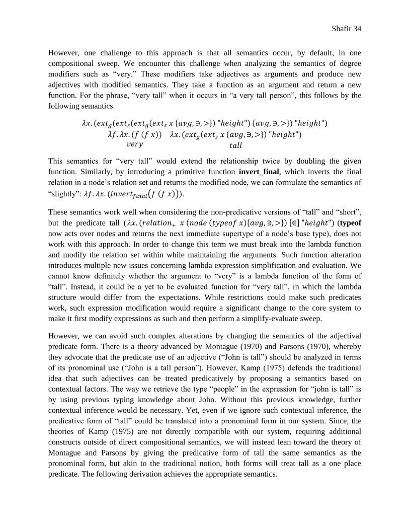
function. For the phrase, “very tall” when it occurs in “a very tall person”, this follows by the

following semantics.

This semantics for “very tall” would extend the relationship twice by doubling the given

function. Similarly, by introducing a primitive function invert_final, which inverts the final

relation in a node‟s relation set and returns the modified node, we can formulate the semantics of

“slightly”: .

These semantics work well when considering the non-predicative versions of “tall” and “short”,

but the predicate tall ( (typeof

now acts over nodes and returns the next immediate supertype of a node‟s base type), does not

work with this approach. In order to change this term we must break into the lambda function

and modify the relation set within while maintaining the arguments. Such function alteration

introduces multiple new issues concerning lambda expression simplification and evaluation. We

cannot know definitely whether the argument to “very” is a lambda function of the form of

“tall”. Instead, it could be a yet to be evaluated function for “very tall”, in which the lambda

structure would differ from the expectations. While restrictions could make such predicates

work, such expression modification would require a significant change to the core system to

make it first modify expressions as such and then perform a simplify-evaluate sweep.

However, we can avoid such complex alterations by changing the semantics of the adjectival

predicate form. There is a theory advanced by Montague (1970) and Parsons (1970), whereby

they advocate that the predicate use of an adjective (“John is tall”) should be analyzed in terms

of its pronominal use (“John is a tall person”). However, Kamp (1975) defends the traditional

idea that such adjectives can be treated predicatively by proposing a semantics based on

contextual factors. The way we retrieve the type “people” in the expression for “john is tall” is

by using previous typing knowledge about John. Without this previous knowledge, further

contextual inference would be necessary. Yet, even if we ignore such contextual inference, the

predicative form of “tall” could be translated into a pronominal form in our system. Since, the

theories of Kamp (1975) are not directly compatible with our system, requiring additional

constructs outside of direct compositional semantics, we will instead lean toward the theory of

Montague and Parsons by giving the predicative form of tall the same semantics as the

pronominal form, but akin to the traditional notion, both forms will treat tall as a one place

predicate. The following derivation achieves the appropriate semantics.

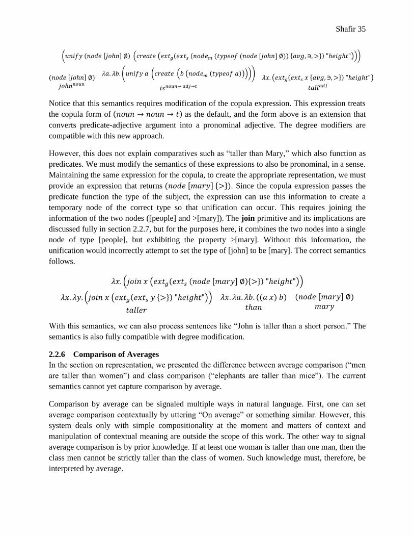
Shafir 35

Notice that this semantics requires modification of the copula expression. This expression treats

the copula form of as the default, and the form above is an extension that

converts predicate-adjective argument into a pronominal adjective. The degree modifiers are

compatible with this new approach.

However, this does not explain comparatives such as “taller than Mary,” which also function as

predicates. We must modify the semantics of these expressions to also be pronominal, in a sense.

Maintaining the same expression for the copula, to create the appropriate representation, we must

provide an expression that returns . Since the copula expression passes the

predicate function the type of the subject, the expression can use this information to create a

temporary node of the correct type so that unification can occur. This requires joining the

information of the two nodes ([people] and >[mary]). The join primitive and its implications are

discussed fully in section 2.2.7, but for the purposes here, it combines the two nodes into a single

node of type [people], but exhibiting the property >[mary]. Without this information, the

unification would incorrectly attempt to set the type of [john] to be [mary]. The correct semantics

follows.

With this semantics, we can also process sentences like “John is taller than a short person.” The

semantics is also fully compatible with degree modification.

2.2.6 Comparison of Averages

In the section on representation, we presented the difference between average comparison (“men

are taller than women”) and class comparison (“elephants are taller than mice”). The current

semantics cannot yet capture comparison by average.

Comparison by average can be signaled multiple ways in natural language. First, one can set

average comparison contextually by uttering “On average” or something similar. However, this

system deals only with simple compositionality at the moment and matters of context and

manipulation of contextual meaning are outside the scope of this work. The other way to signal

average comparison is by prior knowledge. If at least one woman is taller than one man, then the

class men cannot be strictly taller than the class of women. Such knowledge must, therefore, be

interpreted by average.

Shafir 36

Currently, if such knowledge exists, the system will not add the class relationship because it will

be inconsistent with current data. However, if before throwing an inconsistency error, the

relation_add function tried to attempt comparison by average, then we would capture this

inference. If the two nodes being compared are entity nodes or if the average comparison is also

disproven by some data, then the function still throws an inconsistency error. Thus, with this

simple modification, we capture average-based comparison without introducing false inference.

2.2.7 Conjunction

Throughout this discussion of model building semantics, we have developed a unification based

approach. The relation_add function is no longer a part of semantic expressions and has been

replaced by unify. This offers a strong advantage when it comes to modifiers because it means

that prior to unification, we are dealing with node objects and not functions. These objects allow

us to easily extend and modify their properties, while the alternative – disassembling lambda

expressions and modifying them is more difficult, less elegant, and less extensible. However, the

disadvantage to storing these objects is the fact that they don‟t hold any semantics on their own.

This disadvantage surfaces when modeling conjunction. If “taller than John” were a function that

took an argument and added a [>] relation between the argument and John, then we could easily

compose a phrase like “taller than John and shorter than Mary” as a two-step process that adds

two relations to the scalar graph.1

In the current system, “taller than John” expresses a node object, and joining two objects requires

redesign whereas joining two functions does not. Before we can join two nodes, we must think of

what such a compound node would store and how the previous primitives could use it.

The felicity of the phrase “taller than John and smarter than Mary” shows that conjunction can

occur over comparisons on different scales. Therefore, compound nodes should be able to store

nodes on different scales. We can also combine nodes without scales as in “John and Mary.”

Being that nodes are currently scale – ID pairs with the scale optional, we can both standardize

and expand this definition to compound nodes by saying that a node is a collection of scale, ID

pairs with a null scale default. I introduce a new primitive, join, to combine nodes by taking the

union of these properties. In addition, I must alter all the previous primitive functions that

operate over nodes to operate over these collections. This only involves a modification in the

underlying algorithms whereby each process is performed iteratively over all the given nodes. A

key change must occur in the create function whereby the typing of the temporary new item is

determined from the type of the first node in a node collection. The semantics of “and” would

involve the join function and differ depending on the context. We illustrate the variants in the

following example (we leave out null values for simplicity of representation).

1 Note, however, that coordinating “a short man but a tall American” would not be compatible with this approach

because here we are forced to deal with node objects.

Shafir 37

The above semantics for conjunction occur between two noun phrases. Between two adjective

phrases, our semantics must differ.

The expressions “taller than Bill and Mary” and “taller than Bill and taller than Mary” both

reduce to the same expression given this semantics for conjunction. This is appropriate since the

two expressions have same semantic content. This expression for conjunction also captures

underspecified predicates like “tall” that don‟t contain class information. The copula can still

pass this information to the predicate.

Conjunction also occurs in many other contexts, but for the purposes of this work the additional

contexts are not crucial to the model constructing semantics. Hence, I omit them from the

discussion.

2.3 Inference and Question Answering

Now that we have discussed representation and model construction, the final stage is how to

retrieve the information from the model. Inference from the model has already been discussed in

the previous sections because this system does not use an intermediate level of logical

representation to store knowledge and instead stores knowledge in a data model and retrieves it

from that same model. The representation, by construction, handles inference. By performing

inference directly from the model, we skip the need for a separate theorem prover.

Much of the discussion on inference in the previous sections has surfaced with consistency and

informativity checking. The scalar graph disallows adding new relationships that are

uninformative or inconsistent. When relationships are added between two nodes, it checks if a

preexisting relationship already exists, and if so, throws inconsistency and uninformativity errors

as appropriate.

The derived or entailed knowledge of the model can be polled through question answering. By

answering questions, we can test the kinds of inference that the system supports. In this section,

we will develop a semantics for different forms questions in order to demonstrate the reasoning

potential of the system.

2.3.1 Direct Relation Testing

1. Is John tall?

Shafir 38

Example (1) presents a straightforward question that tests whether a specific relationship exists

within the model ( ). The components for this sentence are

identical to the declarative form, and the only semantics that can differ is the copula because its

context differs. The semantics for “tall” performs node relation and graph extension, and the

copula applies that extension to a node. According to the revised system for adjectival predicates

from the previous section, the copula actually creates a temporary node, which it then unifies

with the subject. This temporary node is unnecessary for relationship testing. Instead, when we

have a specific node structure (not necessarily existing in the graph), we can test if the properties

of that node match the properties of a preexisting node. To do this comparison, I introduce a

function compare which takes an existing node and a node structure and compares to see if the

properties of the node structure (its relation set) apply to the existing node. It returns a boolean

value; thus, we will have to add booleans as primitives in the expression language, which we

return as the result of evaluation. The resulting copular semantics are as follows.

2. Is John taller than Mary?

Example (2) follows in much the same way as (1) and the above copula semantics allows this to

work.

3. Is John a tall person?

Example (3) needs a new semantics for the copula in the pronominal context. Here, the

semantics for “a tall person” will create a temporary node, but this temporary node is only for

comparison. I alter the primitive compare so that, prior to returning the Boolean result, it deletes

the temporary node that is the second argument. Comparison still occurs identically to before.

4. Is John taller than Mary and shorter than Bill?

We can capture cases with conjunction as in example (4) by simply allowing the comparison

functions to operate over all the properties of a node. Nodes with multiple properties are

discussed in the conjunction section of model creation.

5. Is John taller than Mary and a tall person?

The semantics of example (5) cannot be captured by the present system. The conjunction of an

adjectival predicate and a pronominal one does not work with the semantics of the copula since it

treats such types differently. However, the felicity of example (5) is questionable, and capturing

this form would require a construct for type-shifting or coercion for the current system to be able

Shafir 39

to capture it. Perhaps it is correct for the grammar to reject these expressions. Nevertheless, the

system can process expressions such as “Is John taller than Mary and tall?”

6. Is John taller than Mary or taller than Bill?

These disjunctive cases do not entail their logical meaning. Returning “yes” to this query does

not make sense. There are multiple possible solutions to this problem. One is to create a new

structure carrying multiple node possibilities and to introduce a new primitive function (or alter

the comparison functions) to choose from amongst those possibilities, the ones true of the first

argument. For reasons of scope, we do not implement of disjunctions of this kind. Storing the

appropriate response involves even deeper modification to the present system.

2.3.2 Set-based Question Answering

The remaining question forms that we will cover are those that return sets of individuals rather

than truth values. This process will involve more revision to the current system.

7. Who is taller than John?

8. Who is taller than John and/but shorter than Mary?

Questions like the one in example (7) deal with sets of nodes, and involve an extension of the

basic graph operations. Example (7) asks for a set of entities that meet two constraints. First,

“who” specifies that the entities must be in the class “people” and second, “taller than John”

specifies that the entities must have a [>] relationship to the node John.

Approaching this problem theoretically, we are searching for the intersection of two sets (the set

of entities taller than John and the set of people). However, such set operations would involve

loading potentially large sets of entities. Instead we will devise an efficient algorithm that will

traverse the scalar graph and filter by type constraints. Example (8) adds additional constraints

on the traversal. For multiple traversal constraints, we will take the intersection of the results.

This algorithm is essentially another graph search algorithm, but this algorithm is not concerned

with finding a target node. It returns all nodes along its traversal path. Additionally, it must

consider the other constraints provided through conjunction and type specification.

Again, I exclude disjunction from the present discussion. Disjunction is compatible with the

current system. We would need a more advanced structure capable of storing conjunction and

disjunction together recursively. However, disjunction does not occur with this intended meaning

in natural language and usage of disjunction in its true logical form surfaces very rarely. In

natural language, “or” often involves very complex semantics that are strongly context-

dependent.

The algorithm that we are building will be provided to the expression language as yet another

primitive function, find. This function takes a node as its argument. This node may be compound

and specifies the constraints on graph traversal. The function returns a set of individuals that

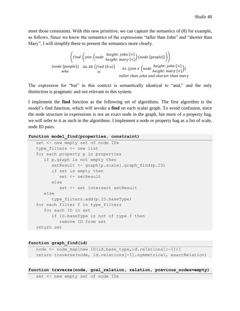
Shafir 40

meet those constraints. With this new primitive, we can capture the semantics of (8) for example,

as follows. Since we know the semantics of the expressions “taller than John” and “shorter than

Mary”, I will simplify these to present the semantics more clearly.

The expression for “but” in this context is semantically identical to “and,” and the only

distinction is pragmatic and not relevant to this system.

I implement the find function as the following set of algorithms. The first algorithm is the

model‟s find function, which will invoke a find on each scalar graph. To avoid confusion, since

the node structure in expressions is not an exact node in the graph, but more of a property bag,

we will refer to it as such in the algorithms. I implement a node or property bag as a list of scale,

node ID pairs.

function model_find(properties, constraint)

set <- new empty set of node IDs

type_filters <- new list

for each property p in properties

if p.graph is not empty then

setResult <- graph[p.scale].graph_find(p.ID)

if set is empty then

set <- setResult

else

set <- set intersect setResult

else

type_filters.add(p.ID.baseType)

for each filter f in type_filters

for each ID in set

if ID.baseType is not of type f then

remove ID from set

return set

function graph_find(id)

node <- node_map[new ID(id.base_type,id.relations[:-1])]

return traverse(node, id.relations[-1].symmetrical, exactRelation)

function traverse(node, goal_relation, relation, previous_nodes=empty)

set <- new empty set of node IDs

Shafir 41

previous_nodes.add(node)

for all edges e from node

if e.node not in previous then

new_relation <- closure(relation,e.relation)

if new_relation <> “X” then

if new_relation = goal_relation then

set.add(e.node)

set.add(traverse(e.node,goal_relation,new_relation,

previous_nodes))

return set

These algorithms are not the most efficient, but they do suffice for the purposes of this system.

They find the set of nodes that satisfy each node property and return the intersection of these

sets. Then, they filter these sets by the type constraint. The primitive expression-language

function calls directly into the model_find algorithm. Using graph traversal, it can retrieve nodes

from scalar graphs that match the criteria set in the natural language query.

3 Further Development

3.1 Negation

Our system can capture and represent input involving negation, but additional complexities make

the semantics more difficult.

1. John is not tall.

Negation of this form seems to act like a degree modifier. The negation of the relation set

is the set . However, treating this set as a class would add the internal

relationships and thus, would reflect the class of people that either neither tall nor average height,

but in-between. This is not the target class. Instead, we want to insert a less than relationship

between “John” and the class of tall people. We are inserting relationships and crucially not

extending nodes (because this would create the aforementioned intermediate class). This means

that negation cannot be interpreted as a degree modifier. Further evidence for this comes in the

syntax rules as shown in the ungrammaticality of example (5).

2. John is a not tall person.*

Therefore, “not” must be part of the semantics of the copula. Furthermore, to deduce the

relationship, we must invert the final relation in the given node‟s relation set. The primitive

function, final_r, returns the final relation in a node‟s relation set, and the primitive function,

invert, returns the inverse of a given relationship. We also will need to retrieve the scale for the

given nodes so I add the scale function to do this. With these new primitives, “not” in the

context [this,adj] and the copula in the context [noun, this, neg] exhibit the following semantics.

Shafir 42

Notice that the copula reverts to its older semantics when working with negation. This is because

unification cannot occur with negation (we cannot unify with a negative). In this way the

semantics support this. Unfortunately, the primitives introduced above only work if the argument

to “not” is a simple node with no coordination. Otherwise, the primitives must work over

multiple scales and multiple relation sets. We need to allow iteration over node properties in the

expression language before such expressions can be captured.

3. John is not a tall person.

To handle example (6), we must undo some of the changes of “a tall person.” It creates a

temporary node that is a member of the “tall people” class. Once this node is created, the only

immediate containment relationship should be to this class. The negation must first retrieve the

node‟s immediate parent class and then remove the temporary node. We introduce a new

primitive function remove, which removes a node and returns its immediate parent. Using this

new primitive we can model the negation semantics in the context [this,noun]

For the above, not only do we need additional constructs to support conjunction like above, but

we also need a construct that makes sure node removal happens only once. We need to ensure

that (remove b) occurs before it is substituted into the lambda expression. These extensions are

outside of the provided implementation and would involve significant revision to the lambda

expression engine.

Additionally, negation exhibits very odd semantic effects depending on its use. Consider

example (4) for instance.

4. John is not very tall.

Instead of the meaning that the above discussion would assume, this negation makes its

argument assume the opposite, namely, “short”. Such odd effects reveal an underlying

complexity in the semantics of negation in scalar expressions that warrants future analysis.

3.2 Quantitative Modeling

The system discussed up to this point does not yet provide a complete degree mapping semantics

because it does not support representation or inference over quantitative data. The scales have

been relational only and as such, the semantics and even the inference logic cannot be complete.

Therefore, we discuss techniques for extending the present system to capture quantitative data.

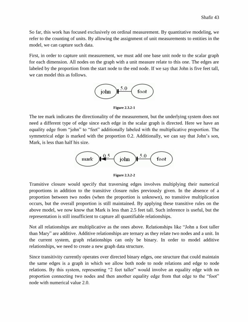
Shafir 43

So far, this work has focused exclusively on ordinal measurement. By quantitative modeling, we

refer to the counting of units. By allowing the assignment of unit measurements to entities in the

model, we can capture such data.

First, in order to capture unit measurement, we must add one base unit node to the scalar graph

for each dimension. All nodes on the graph with a unit measure relate to this one. The edges are

labeled by the proportion from the start node to the end node. If we say that John is five feet tall,

we can model this as follows.

Figure 2.3.2-1

The tee mark indicates the directionality of the measurement, but the underlying system does not

need a different type of edge since each edge in the scalar graph is directed. Here we have an

equality edge from “john” to “feet” additionally labeled with the multiplicative proportion. The

symmetrical edge is marked with the proportion 0.2. Additionally, we can say that John‟s son,

Mark, is less than half his size.

Figure 2.3.2-2

Transitive closure would specify that traversing edges involves multiplying their numerical

proportions in addition to the transitive closure rules previously given. In the absence of a

proportion between two nodes (when the proportion is unknown), no transitive multiplication

occurs, but the overall proportion is still maintained. By applying these transitive rules on the

above model, we now know that Mark is less than 2.5 feet tall. Such inference is useful, but the

representation is still insufficient to capture all quantifiable relationships.

Not all relationships are multiplicative as the ones above. Relationships like “John a foot taller

than Mary” are additive. Additive relationships are ternary as they relate two nodes and a unit. In

the current system, graph relationships can only be binary. In order to model additive

relationships, we need to create a new graph data structure.

Since transitivity currently operates over directed binary edges, one structure that could maintain

the same edges is a graph in which we allow both node to node relations and edge to node

relations. By this system, representing “2 feet taller” would involve an equality edge with no

proportion connecting two nodes and then another equality edge from that edge to the “foot”

node with numerical value 2.0.

Shafir 44

Such a structure brings up many questions about model minimization and scalar inference. There

are many new forms of inference involving additive and multiplicative quantitative data

combined with the relational data from before. There is no longer necessarily a single way to

retrieve the relationship between two nodes. Inference can no longer follow entirely from

transitive rules and instead, the system must operate over constraints, attempting to find a

possible assignment of values that satisfies all the constraints. If John is two feet taller than Bill

and also twice Bill‟s height, we know that John is four feet tall. This kind of inference is indirect

and occurs by the solving the set of constraints on the node‟s numeric data. A solution to this

dilemma remains outside the scope of this work, but it is an important area of knowledge

inference for future research.

3.3 Measurement Sensitivity

The system discussed in this work assumes a perfection of measurement that does not exist in the

physical world. The fact that two people are of equivalent height can only be true up to a certain

point of sensitivity. Realistically, no two individuals can be exactly the same height. As noted in

(Krantz et al. 1971), when two entities are too similar, any method of comparing them

deteriorates. Furthermore, even units of measurement are observed inaccurately with respect to a

higher degree of sensitivity.

Comparing the heights of ants, for instance, involves a much greater degree of sensitivity than

comparing human heights. In order for a system to accurately model data, it must maintain a

shifting measurement sensitivity threshold by class and context of discussion. In the end, every

system must approximate to some degree.

3.4 Quantitative Adjustment and Classification

Adding unit measurement to the modeling capabilities of this system provides more benefits than

the ones outlined in section 3.2. By performing additional adjustments, we can construct a

system that, through automatic machine learning, will scale to better capture real data.

When discussing relational modeling, we introduced a new relation, average, that was exactly

like contains, but different only in name. The purpose of this was so that class nodes could

distinguish which containment edge held the average node for that class. With this knowledge,

we can now target the average node of each class for adjustment when new members are added

to that class. Whenever a node with a unit measurement is added to the scalar graph, we adjust

the averages of each of the containing classes and create new average nodes when they do not

exist. This adjusted average will now affect inferences drawn from the data. We know, for

instance that all tall people are taller than the average for the people class, and since we adjust

this average, we can know at least the minimal threshold for all tall people.

Furthermore, from knowing the unit values of the members of any given class, we can use

machine learning to create a classifier capable of sorting new entities into that class. We feed the

known values to the classifier as training data and use the output model to classify new instances

Shafir 45

of a class into the derived subclasses. For instance, from collect data on the heights of tall people,

we can classify new people as in or out of the class “tall.” The data given to the classifier

contains only a single feature (the unit value).

Support vector machines (SVMs) (developed from Vapnik & Lerne 1963) would be very useful

in this learning task. SVMs create a hyperplane that best splits the positive and negative samples.

The best hyperplane is the one that maintains the maximum margin from the positive and

negative samples. However, a linear hyperplane would not be able to separate “average-height

people” from “short” and “tall” since this data has two thresholds. Bosner, Guyon, & Vapnik

(1992) propose a method of creating a nonlinear hyperplane classifier by applying the kernel

trick (Aizerman et al. 1964). This allows the classifier to fit the maximum-margin hyperplane in

a transformed feature space where the transformation may be nonlinear and the transformed

space may be high dimensional. To illustrate this process, imagine we mark positive and

negative samples for “average person height” on a one dimensional line. We can separate the

positive samples from the negative ones by with a radial basis function in a transformed two

dimensional feature space. Using a gaussian radial basis function as the kernel function, an SVM

classifier will be able to learn class thresholds and classify new data into classes.

The data given to the classifier will include entity samples as well as instances of the average to

account for unattested data. The more data that the system models, the more accurate its

classification will be and thus, the system will scale to acquire general world knowledge through

specific samples.

3.5 Multidimensionality

The current system can handle representation and inference for multiple independent dimensions

or scales. However, scales are often interdependent. For instance, the length and height of a

building contribute to its overall size. The semantics for a word like “size” cannot be properly

modeled without a system capable of representing dependencies between scales.

To further complicate the matter, scales have different dependencies on different ends and for

different classes. Consider how “small” refers to the lower end of both scales on height and size,

while “tall” and “big” are sometimes distinct depending on the class of comparison.

Modeling such interdependencies will prove useful for the quantitative classification techniques

discussed in the previous section. Classes that depend on multiple scales can pass values along

all their dimensions as separate features and SVM will find the threshold to best surround the

data. Such multidimensional classification can have many practical benefits and allows an

entirely new form of knowledge-based inference.

3.6 Scale Resolution and Lexical Semantics

This work omits discussion of lexical semantics as it relates to scalar modeling. However, many

gradable predicates cannot be interpreted without lexical decomposition. In a previous work, I

examined how the adjective “good” derives its semantics from the lexical decomposition of its

Shafir 46

argument. Many “adjectives” are like “good” and unspecified with respect to the scale they

operate over. Instead, the scale must be inferred from the arguments being compared.

Consider the phrase “a long road”, “long,” unlike the predicate “tall,” does not specify the scale

of its argument. Instead it must infer the best scale from the lexical semantics of the word “road”

and from its own lexical semantics.

The Generative Lexicon Theory (Pustejovsky 1995) provides a framework for modeling lexical

semantics. In our system we can model the qualia structure of the items in our lexicon. The

underspecified adjectival predicates will then make use of this qualia structure in inferring the

appropriate scale for a given entity or class.

We give an example to illustrate this process. Consider that “length” refers to scales of span

(time span, physical span, etc.) where a value begins at a point along a continuum and ends at

another point and we measure the interval between the two points. A road would have a property

for physical span in its formal quale. A meeting would have a property for time span in its formal

quale. “Length” would look for varying spans in the formal quale of its argument. These span

elements in the qualia structure would refer to scales in the model and thus, we would be able to

retrieve and model variations in these formal properties.

The cases for scale resolution are not always as simple as the examples above. Consider how

“length” acts over the argument “day.” Since “day” has a fixed time span, length cannot choose

this as the scale. Intuitively, we understand that a “long day” must be a day perceived as long –

usually through multiple patience-testing events. The inference needed to construct this

semantics is beyond the scope of lexical decomposition alone. “Long” tries to coerce its

argument to have a time span since this is only span available at its disposal. This coercion

attaches an experiencer to the concept of a day and thus the rigid formal properties become

subjective.

Creating an extensible framework capable of such coercion is challenging and requires

considering many adjectives independently because adjectives have widely differing schemes for

inferring the appropriate relation scale. Generalizing these schemes into a core set of primitives

and embedding those primitives in the expression language will allow this system to capture the

semantics of these gradable predicates.

4 Conclusion

This work presents the foundation for a computational method of capturing scalar semantic

content. In order for this foundation to support extension, much thought has gone into its

implementation. Many subtleties in the semantics had to be resolved before such a system could

properly capture even simple entailments. However, with such a framework in place, the

potential for future research expands. Even the extensions discussed above do not put forth a

complete list. This work omits discussion of superlatives, pragmatic and contextual effects, type

Shafir 47

coercion, and efficiency, to name a few. Nevertheless, the system provides a simple basis upon

which new features can be built.

In addition to providing a basis, a computational framework presents an objective ordering of the

prominent issues at hand. From evaluating what data the system can and cannot capture, one can

discern the more evident weaknesses and approach these issues based on both their theoretical

and practical viability. Stechow (1984) reevaluates existing semantic theories of comparison

based on the data and entailments that they can logically capture, but the principles laid forth in

this work allow for a further reevaluation that considers the computational efficiency of the

differing approaches. This can help to focus future research.

This work can also help to advance research in computational linguistics. With this basis, scalar

information extraction can become a feasible task. And classifying scalar categories is an

appropriate application of machine learning. Such work can help to unify research in theoretical

semantics with that of statistical, computational linguistics.

Shafir 48

5 Bibliography Aizerman, M., Braverman, E., & Rozonoer, L. (1964). Theoretical foundations of the potential

function method in pattern recognition learning. Automation and Remote Control, 25,

821–837.

Barendregt, H., & Barendsen, E. (2000, March). Introduction to Lambda Calculus. Retrieved

from ftp://ftp.cs.ru.nl/pub/CompMath.Found/lambda.pdf

Bartsch, R., & Vennemann, T. (1972). The grammar of relative adjectives and comparison.

Linguistische Berichte(20), 19–32.

Bartsch, R., & Vennemann, T. (1973). Semantic structures: A study in the relation between

syntax and semantics. Frankfurt: Athaenum Verlag.

Bierwisch, M. (1989). The Semantics of gradation. In M. Bierwisch, & E. Lan (Eds.),

Dimensional Adjectives (pp. 71-261). Berlin: Springer-Verlag.

Blackburn, P., & Bos, J. (2005). Representation and Inference for Natural Language. CSLI

Publications.

Boguslawski, A. (1975). Measures are measures: In defence of the diversity of comparatives and

positives. Linguistiche Berichte(36), 1–9.

Boser, B. E., Guyon, I. M., & N, V. V. (1992). A training algorithm for optimal margin

classifiers. In D. Haussler (Ed.), 5th Annual ACM Workshop on COLT (pp. 144–152).

Pittsburgh, PA: ACM Press.

Cresswell, M. J. (1977). The semantics of degree. In B. Partee (Ed.), Montague Grammar (pp.

261-292). New York: Academic Press.

Heim, I. (1985). Notes on comparatives and related matters. Ms., University of Texas.

Heim, I. (2000). Degree operators and scope. In B. Jackson, & T. Matthew (Eds.), Semantics and

Linguistic Theory (Vol. 10, pp. 40-64). Ithaca, NY: CLC Publication.

Hellan, L. (1981). Towards an integrated analysis of comparatives. Tubingen: Narr.

Jacobson, P. (2006, February 25). Direct compositionality and variable free semantics: Taking

the surprise out of ‘‘complex variables’’. Lecture at the 30th Penn Linguistics

Colloquium, University of Pennsylvania, February 25, 2006.

Kamp, H. (1975). Two theories of adjectives. In E. Keenan (Ed.), Formal semantics of natural

language (pp. 123–155). Cambridge: Cambridge University Press.

Shafir 49

Kennedy, C. (1997). Projecting the adjective: The syntax and semantics of gradability and

comparison. New York: Garland.

Kennedy, C. (2001). Polar opposition and the ontology of „degrees‟. Linguistics and

Philosophy(24), pp. 33-70.

Kennedy, C. (2007). Vagueness and Grammar: the semantics of relative and absolute gradable

adjectives. Linguist Philos(30), 1-45.

Kennedy, C., & McNally, L. (2005). Scale structure and the semantic typology of gradable

predicates. Language, 81(2), pp. 345-381.

Klein, E. (1980). A Semantics for Positive and Comparative Adjectives. Linguistics and

Philosophy(4), 1-45.

Klein, E. (1991). Comparatives. In A. von Stechow, & D. Wunderlic (Eds.), Semantik: Ein

internationales Handbuch der zeitgenossischen Forschung (pp. 673-691). Berlin: Walter

de Gruyter.

Krantz, D. H., Luce, D. R., Suppes, P., & Tversky, A. (1971). Foundations of Measurement

(Vol. I). New York: Academic Press, Inc.

Montague, R. (1973). The Proper Treatment of Quantification in Ordinary English. (R. H.

Thomason, Ed.)

Parsons, T. (1970). Some Problems Concerning the Logic of Grammatical Modifiers. Synthese,

21, 320-334.

Partee, B., Meulen, A. G., & Wall, R. E. (1990). Mathematical Methods in linguistics. Dodrecht:

Kluwer Academic Publishers.

Pustejovksy, J. (1995). The Generative Lexicon. Cambridge, MA: MIT Press.

Seuren, P. A. (1973). The comparative. In K. F, & R. N (Eds.), Generative grammar in Europe

(pp. 528-564). Dordrecht: Reidel.

Stanley, J. (2000). Context and logical form. Linguistics and Philosophy, 23(4), 391–434.

Stechow, A. v. (1984). Comparing semantic theories of comparison. Journal of Semantics(3), 1-

77.

Tye, M. (1994). Sorites paradoxes and the semantics of vagueness. In J. E. Tomberlin (Ed.),

Philosophical Perspectives 8: Logic and Language (pp. 189-206). Atascadero, CA:

Ridgeview Publishing Co.

Shafir 50

Vapnik, V., & Lerne, A. (1963). Pattern recognition using generalized portrait method.

Automation and Remote Control(24), 774-780.