Scalable Digital Architecture of a Liquid State Machine
85
Rochester Institute of Technology Rochester Institute of Technology RIT Scholar Works RIT Scholar Works Theses 5-8-2017 Scalable Digital Architecture of a Liquid State Machine Scalable Digital Architecture of a Liquid State Machine Anvesh Polepalli [email protected] Follow this and additional works at: https://scholarworks.rit.edu/theses Recommended Citation Recommended Citation Polepalli, Anvesh, "Scalable Digital Architecture of a Liquid State Machine" (2017). Thesis. Rochester Institute of Technology. Accessed from This Thesis is brought to you for free and open access by RIT Scholar Works. It has been accepted for inclusion in Theses by an authorized administrator of RIT Scholar Works. For more information, please contact [email protected].
Transcript of Scalable Digital Architecture of a Liquid State Machine

Rochester Institute of Technology Rochester Institute of Technology
RIT Scholar Works RIT Scholar Works
Theses
5-8-2017
Scalable Digital Architecture of a Liquid State Machine Scalable Digital Architecture of a Liquid State Machine
Anvesh Polepalli [email protected]
Follow this and additional works at: https://scholarworks.rit.edu/theses
Recommended Citation Recommended Citation Polepalli, Anvesh, "Scalable Digital Architecture of a Liquid State Machine" (2017). Thesis. Rochester Institute of Technology. Accessed from
This Thesis is brought to you for free and open access by RIT Scholar Works. It has been accepted for inclusion in Theses by an authorized administrator of RIT Scholar Works. For more information, please contact [email protected].

Scalable Digital Architecture of a
Liquid State Machine
Anvesh Polepalli

Scalable Digital Architecture of a
Liquid State MachineAnvesh Polepalli
May 8, 2017
A Thesis Submittedin Partial Fulfillment
of the Requirements for the Degree ofMaster of Science
inComputer Engineering
Department of Computer Engineering

Scalable Digital Architecture of a
Liquid State MachineAnvesh Polepalli
Committee Approval:
Dr. Dhireesha Kudithipudi Advisor DateAssociate Professor
Dr. Marcin Lukowiak DateAssociate Professor
Dr. Ernest Fokoue DateAssociate Professor
i

Acknowledgments
I avail this opportunity to express my sincere gratitude to my thesis advisor Dr.
Dhireesha Kudithipudi for her valuable support and motivation. I thank Dr.Marcin
Lukowiak and Dr.Ernest Fokoue for serving on my thesis committee and their in-
sightful comments and encouragement.
I also express my hearty thanks to Dr. Mark Indovina for his help in setting up
the environment for using synopsys tools.
I thank my labmates Qutaiba Mohammed Saleh, Nicholas Soures, Michael Foster,
Swathika Ramakrishnan and Sadhvi Praveen for their guidance and the stimulating
discussions.
I extend my profound thanks to all the faculty members of my department for
the technical knowledge provided which greatly helped me in accomplishing the work
successfully.
I am greatly indebted to my parents and friends for their wholehearted support
which made it possible for me to successfully complete this thesis in time.
ii

To my dad, mom and loving bother who supported me along the way.
iii

Abstract
Scalable Digital Architecture of a Liquid State Machine
Anvesh Polepalli
Supervising Professor: Dr. Dhireesha Kudithipudi
Liquid State Machine (LSM) is an adaptive neural computational model with rich
dynamics to process spatio-temporal inputs. These machines are extremely fast in
learning because the goal-oriented training is moved to the output layer, unlike con-
ventional recurrent neural networks.
The capability to multiplex at the output layer for multiple tasks makes LSM a
powerful intelligent engine. These properties are desirable in several machine learning
applications such as speech recognition, anomaly detection, user identification etc.
Scalable hardware architectures for spatio-temporal signal processing algorithms like
LSMs are energy efficient compared to the software implementations. These designs
can also naturally adapt to different temporal streams of inputs. Early literature
shows few behavioral models of LSM. However, they cannot process real time data
either due to their hardware complexity or fixed design approach. In this thesis, a
scalable digital architecture of an LSM is proposed. A key feature of the architecture
is a digital liquid that exploits spatial locality and is capable of processing real time
data. The quality of the proposed LSM is analyzed using kernel quality, separation
property of the liquid and Lyapunov exponent. When realized using TSMC 65nm
technology node, the total power dissipation of the liquid layer, with 60 neurons, is
55.7 mW with an area requirement of 2mm2. The proposed model is validated for two
benchmark. In the case of an epileptic seizure detection an average accuracy of 84%
is observed. For user identification/authentication using gait an average accuracy of
98.65% is achieved.
iv

Contents
Signature Sheet i
Acknowledgments ii
Dedication iii
Abstract iv
Table of Contents v
List of Figures viii
List of Tables x
1 Introduction 1
1.1 Motivation . . . . . . . . . . . . . . . . . . . . . . . . . . . . . . . . . 1
1.2 Objectives . . . . . . . . . . . . . . . . . . . . . . . . . . . . . . . . . 3
1.3 Outline . . . . . . . . . . . . . . . . . . . . . . . . . . . . . . . . . . . 4
2 Background and Related Work 5
2.1 Introduction to Neurons . . . . . . . . . . . . . . . . . . . . . . . . . 5
2.1.1 McCulloch-Pitts . . . . . . . . . . . . . . . . . . . . . . . . . . 5
2.1.2 Continuous Activation Function Neurons . . . . . . . . . . . . 7
2.1.3 Spiking Neurons . . . . . . . . . . . . . . . . . . . . . . . . . . 8
2.2 Introduction to Recurrent Neural Networks (RNNs) . . . . . . . . . . 10
2.2.1 Echo State Network (ESN) . . . . . . . . . . . . . . . . . . . . 11
2.2.2 Liquid State Machine (LSM) . . . . . . . . . . . . . . . . . . 11
2.3 LSM Algorithm . . . . . . . . . . . . . . . . . . . . . . . . . . . . . . 12
2.4 Training Example . . . . . . . . . . . . . . . . . . . . . . . . . . . . . 15
2.5 Applications . . . . . . . . . . . . . . . . . . . . . . . . . . . . . . . . 20
2.5.1 Epileptic Seizure Detection . . . . . . . . . . . . . . . . . . . . 20
2.5.2 Biometric User Identification/Verification . . . . . . . . . . . . 20
2.6 Related Work . . . . . . . . . . . . . . . . . . . . . . . . . . . . . . . 21
2.7 Summary . . . . . . . . . . . . . . . . . . . . . . . . . . . . . . . . . 23
v

CONTENTS
3 Proposed Design 24
3.1 Proposed Behavioral Design Overview . . . . . . . . . . . . . . . . . 24
3.1.1 Preprocessing . . . . . . . . . . . . . . . . . . . . . . . . . . . 24
3.1.2 Input Layer . . . . . . . . . . . . . . . . . . . . . . . . . . . . 26
3.1.3 Connection from Input Layer to Liquid . . . . . . . . . . . . . 26
3.1.4 Liquid Layer . . . . . . . . . . . . . . . . . . . . . . . . . . . . 28
3.1.5 Liquid to Output Layer . . . . . . . . . . . . . . . . . . . . . 30
3.1.6 Output Layer . . . . . . . . . . . . . . . . . . . . . . . . . . . 31
3.2 Liquid Topologies . . . . . . . . . . . . . . . . . . . . . . . . . . . . . 33
3.2.1 Random Topology . . . . . . . . . . . . . . . . . . . . . . . . 33
3.2.2 Spatial Topology . . . . . . . . . . . . . . . . . . . . . . . . . 33
3.3 Summary . . . . . . . . . . . . . . . . . . . . . . . . . . . . . . . . . 34
4 Digital Design 35
4.1 Pre-Processing . . . . . . . . . . . . . . . . . . . . . . . . . . . . . . 36
4.2 Liquid . . . . . . . . . . . . . . . . . . . . . . . . . . . . . . . . . . . 36
4.2.1 Weighted Current Block . . . . . . . . . . . . . . . . . . . . . 38
4.2.2 Integrator Block . . . . . . . . . . . . . . . . . . . . . . . . . . 39
4.2.3 Spike Generator Block . . . . . . . . . . . . . . . . . . . . . . 41
4.2.4 Spike Counter Block . . . . . . . . . . . . . . . . . . . . . . . 42
4.3 Output Layer . . . . . . . . . . . . . . . . . . . . . . . . . . . . . . . 42
4.4 Summary . . . . . . . . . . . . . . . . . . . . . . . . . . . . . . . . . 45
5 Spatio-temporal Datasets 46
5.1 Data Sets . . . . . . . . . . . . . . . . . . . . . . . . . . . . . . . . . 46
5.1.1 Epilepsy . . . . . . . . . . . . . . . . . . . . . . . . . . . . . . 47
5.1.2 User Verification Using Biometric Walking Pattern . . . . . . 47
5.2 Summary . . . . . . . . . . . . . . . . . . . . . . . . . . . . . . . . . 50
6 Results and Analysis 51
6.1 Applications . . . . . . . . . . . . . . . . . . . . . . . . . . . . . . . . 51
6.1.1 Epileptic Seizure Detection . . . . . . . . . . . . . . . . . . . . 51
6.1.2 User Identification/Authentication using Walking Patterns . . 56
6.2 Reservoir Metrics . . . . . . . . . . . . . . . . . . . . . . . . . . . . . 58
6.2.1 Kernel quality . . . . . . . . . . . . . . . . . . . . . . . . . . . 58
6.2.2 Separation Property of the Liquid . . . . . . . . . . . . . . . . 59
6.2.3 Lyapunov Exponent . . . . . . . . . . . . . . . . . . . . . . . 60
vi

CONTENTS
6.3 Power and Area . . . . . . . . . . . . . . . . . . . . . . . . . . . . . . 61
7 Conclusion and Future Work 63
7.1 Conclusion . . . . . . . . . . . . . . . . . . . . . . . . . . . . . . . . . 63
7.2 Future Work . . . . . . . . . . . . . . . . . . . . . . . . . . . . . . . . 64
vii

List of Figures
2.1 McCulloch-Pitts (or first generation) neuron model. . . . . . . . . . . 6
2.2 Continuous activation function (or second generation) neuron model. 7
2.3 Spiking neuron (or third generation) model. . . . . . . . . . . . . . . 9
2.4 Basic structure of LSM. . . . . . . . . . . . . . . . . . . . . . . . . . 14
2.5 Input test signal. . . . . . . . . . . . . . . . . . . . . . . . . . . . . . 15
2.6 Liquid response (spike count) for the input shown in figure 2.5. . . . . 16
2.7 Liquid response; output voltage of each neuron with respect to time
varying input (test signal with frequency F1 - 4Hz shown in figure 2.5). 16
2.8 Liquid response; output voltage of each neuron with respect to time
varying input (test signal with frequency F2 - 1Hz shown in figure 2.5). 17
2.9 Liquid response; output current of each neuron with respect to a time
varying input (test signal with frequency F1 - 4Hz. . . . . . . . . . . 17
2.10 Liquid response; output current of each neuron with respect to a time
varying input (test signal with frequency F2 - 1Hz. . . . . . . . . . . 18
2.11 Confusion matrix. . . . . . . . . . . . . . . . . . . . . . . . . . . . . . 18
2.12 Confusion matrix indicating accuracies of training, testing and validation. 19
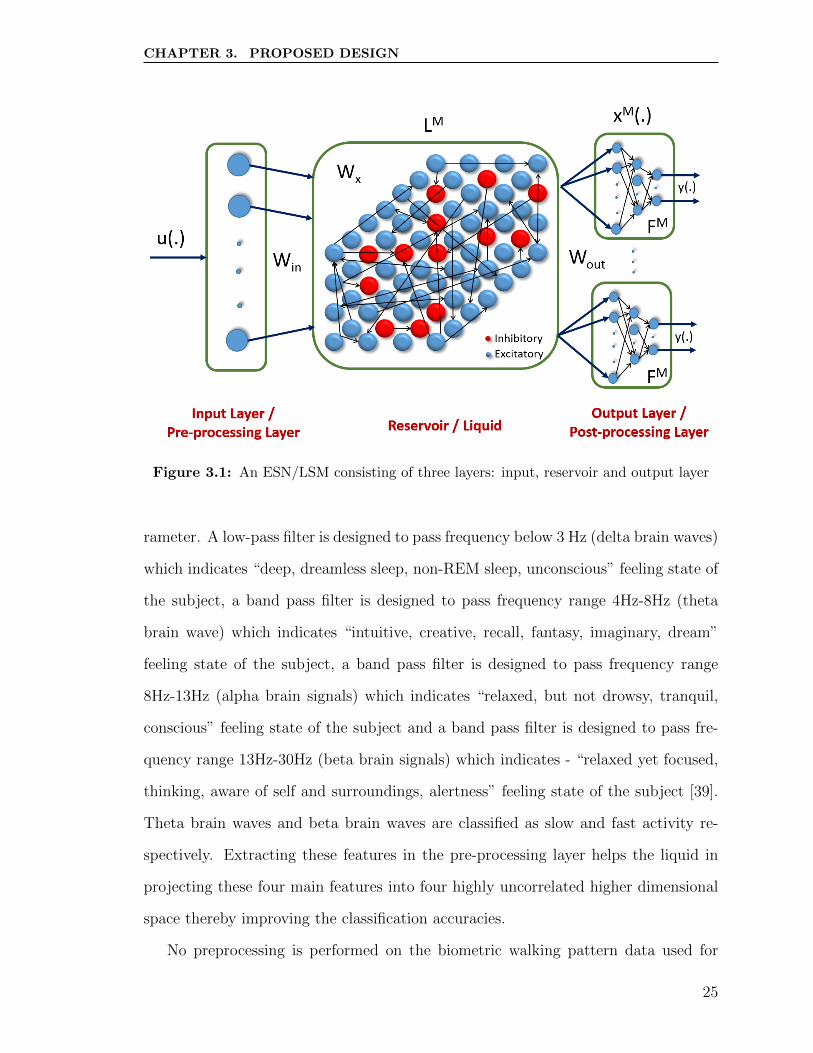
3.1 An ESN/LSM consisting of three layers: input, reservoir and output
layer . . . . . . . . . . . . . . . . . . . . . . . . . . . . . . . . . . . . 25
3.2 Output Layer of the LSM as a Multilayer Perceptron) . . . . . . . . . 32
4.1 Architecture of LSM. . . . . . . . . . . . . . . . . . . . . . . . . . . . 35
4.2 Filter response in the input layer. . . . . . . . . . . . . . . . . . . . . 37
4.3 Leaky Integrate-and-fire neuron Model. . . . . . . . . . . . . . . . . . 38
4.4 Weighted current block of Leaky-Integrate-and-Fire (LIF) neuron model. 39
4.5 Integrator block of LIF neuron model . . . . . . . . . . . . . . . . . . 40
4.6 Spike generator block of LIF neuron model . . . . . . . . . . . . . . . 42
4.7 Output layer of LSM . . . . . . . . . . . . . . . . . . . . . . . . . . . 43
4.8 IEEE754 Single precision 32-bit . . . . . . . . . . . . . . . . . . . . . 43
4.9 Input to output comparison between sigmoid and piece-wise sigmoid
functions . . . . . . . . . . . . . . . . . . . . . . . . . . . . . . . . . . 44
5.1 Electrode placements [1]. . . . . . . . . . . . . . . . . . . . . . . . . . 48
viii
LIST OF FIGURES
5.2 Time series EEG signal samples for (a) Normal case (dataset A) and
(b) Seizure case (dataset E). . . . . . . . . . . . . . . . . . . . . . . 48
5.3 Accelerometer Recordings in XYZ Coordinates for two individuals. . . 49
6.1 Response of the 4 FIR filters in the input layer for the Electroencephalography
(EEG) signals as presented in figure 5.2a. . . . . . . . . . . . . . . . . 52
6.2 Response of the 4 FIR filters in the input layer for the EEG signals as
presented in figure 5.2b. . . . . . . . . . . . . . . . . . . . . . . . . . 52
6.3 Liquid response for EEG signals. . . . . . . . . . . . . . . . . . . . . 53
6.4 Liquid response for EEG signals. . . . . . . . . . . . . . . . . . . . . 53
6.5 Cross-Entropy vs Epochs for epileptic seizure detection. . . . . . . . . 55
6.6 Confusion matrix based on the predictions made by the LSM for epilep-
tic seizure detection. . . . . . . . . . . . . . . . . . . . . . . . . . . . 55
6.7 Normalized accelerometer readings along x,y,z axis for subject 1. . . . 56
6.8 Normalized accelerometer readings along x,y,z axis for subject 2. . . . 56
6.9 Cross-Entropy vs Epochs for user identification/authentication. . . . 57
6.10 Confusion matrix based on the predictions made by the LSM for user
identification/authentication. . . . . . . . . . . . . . . . . . . . . . . 57
6.11 Lyapunov Exponent for reservoir performance on different tasks. . . . 60
ix

List of Tables
2.1 Comparison of various spiking neuron models. NOTE: #of Floating-
point Operations Per Second (FLOPS) is an approximate number of
floating point operations (addition, multiplication, etc.) needed to
simulate the model for one time step as referred in [2]. . . . . . . . . 10
6.1 Area estimates of the liquid for different TSMC technology nodes. . . 61
6.2 Power consumption of the liquid at different TSMC technology node. 61
6.3 Power estimates of the liquid on a Xilinx Vertex6 VSX315TL FPGA
board. . . . . . . . . . . . . . . . . . . . . . . . . . . . . . . . . . . . 61
6.4 Area estimates of the liquid on a Xilinx Vertex6 VSX315TL FPGA
board. . . . . . . . . . . . . . . . . . . . . . . . . . . . . . . . . . . . 62
6.5 Area estimates of the Pre-processing block on a Xilinx Vertex6 VSX315TL
FPGA board. . . . . . . . . . . . . . . . . . . . . . . . . . . . . . . . 62
6.6 Area estimates of the output block on a Xilinx Vertex6 VSX315TL
FPGA board. . . . . . . . . . . . . . . . . . . . . . . . . . . . . . . . 62
x

Chapter 1
Introduction
1.1 Motivation
Many real-world phenomena of interest in various applications such as speech recog-
nition, bio-signal processing, biometric user verification (via speech/walking style),
visual stimuli etc. are spatio-temporal in nature. For example, epilepsy detection
from EEG data. Only by continuous processing of these spatio-temporal signals,
we are able to perceive, predict, or identify patterns. It is anticipated that next-
generation autonomous systems have similar behavior, where they rely on memory
of recent states to process spatio-temporal streams of information and find correla-
tions in patterns so that predictions can be made based on these dynamic signals.
Observing these spatio-temporal signals at one specific time step does not provide
enough information for predictions. Predictions should be made based not only on
the current input but also considering the inputs from previous time steps. Rather,
the knowledge of events in a temporal window enables efficient predictions which
are highly task/data dependent i.e. the duration of the window to be observed to
predict/classify is task dependent.
An important question is information from how many specific previous time steps
is required at any given time? Several ongoing research efforts focus on developing
algorithms to address the problems of processing spatio-temporal signals. Few of the
1

CHAPTER 1. INTRODUCTION
current generation Neural Networks (NNs) address this issue. Training Recurrent
Neural Networks (RNNs) is computationally expensive using methods such as back-
propagation through time. They also suffer from exploding and vanishing gradients
and are computationally expensive [3]. A class of networks known as Reservoir Com-
puting (RC) that were proposed in 2002, offer rapid training capability. Liquid State
Machine (LSM), belonging to RC framework, is one such algorithm (or dynamical
system) that is gaining lot of attention in this realm. Unlike other machine learning
algorithms RCs are not trained by gradient-descent-based methods, which aim at
iteratively reducing the training error. More importantly the fading memory within
the reservoir does not require a predefined temporal window. There are two parallel
efforts that emerged in RC - Echo State Networks (ESNs) [4], inspired from the field
of Machine Learning (ML), and LSMs [5], inspired from computational neuroscience.
Both approaches share the same basic idea of having a reservoir that projects the
inputs onto a nonlinear higher dimensional space followed by a simple readout mech-
anism, which reads the state of the reservoir and maps it to the desired class by
extracting only the desired features (section 2.2 provides further details).
The recurrent connections of the reservoir layer enable extracting desired features,
by explicitly storing information from previous time-steps, along with current input
to make predictions. LSM, is based on a rigorous mathematical framework [5]. LSMs
have universal computational power for real time processing with fading memory
property [5]. LSMs employ a simple training algorithm compared to other types of
RNNs which use back propagation and gradient descent methods. The advantage of
the training algorithm is that the weights (or synapse strength) connecting neurons
within the liquid are not updated during training; they remain at their initial state,
but only the weights in the output layer are updated during training.
Software models of LSM have been implemented in diverse applications such as
facial expression recognition [6], speech recognition [7], and isolated word recognition
2

CHAPTER 1. INTRODUCTION
[8]. In general, digital hardware realization of LSM offers performance and energy
efficiency [9], [10], [11], and [12] due to the homogeneous and multitude synaptic
connections of the reservoir that lead to a highly parallel architecture. In literature,
there are a few proposed LSM architectures such as the ‘compact hardware on FPGA’
[13], ‘hardware efficient neuromorphic dendritically enhanced readout’ [14], ‘real-time
speech recognition’ [15]. None of these models have a fully integrated architecture for
processing spatio-temporal signals. There are a few memristor based architectures
that are also proposed for the ESN and validated for bio-signal processing signals
[16], which do not work with the spiking LSM reservoirs.
This thesis focuses on design and implementation of a scalable digital LSM, with
low power dissipation while processing real time signals.
1.2 Objectives
The specific objectives of this research are:
• Develop a behavioral/software LSM model for baseline analysis.
• Explore various design parameters that can optimize the baseline LSM model,
considering hardware design complexity.
• Validate the baseline LSM model on two different spatio-temporal datasets.
– Epileptic seizure detection [1].
– User identification/authentication with gait patterns [17].
• Optimized end-to-end digital hardware architecture of the LSM with pre and
post processing.
• Validate the hardware model with two spatio-temporal data sets and study the
power profile and area requirement.
3

CHAPTER 1. INTRODUCTION
1.3 Outline
The reset of this document is outlined as follows Chapter 2 provides an introduction
to generation of neurons, RC, LSM training algorithm and an example to demon-
strate the performance of LSM. Chapter 3 presents the proposed LSM model and
its architecture. Chapter 4 provides the overview of a reconfigurable digital design of
the LSM. Chapter 5 provides the datasets used to benchmark the proposed design.
Chapter 6 presents the benchmarking results of the proposed design for datasets pre-
sented in chapter 5 and metric analysis. Chapter 7 discusses conclusions and future
work.
4

Chapter 2
Background and Related Work
2.1 Introduction to Neurons
Artificial neuron is a computational model based on the structure and functions of bi-
ological neuron. Artificial neuron’s are the basic computational units in any Artificial
Neural Networks (ANNs). Neuron receives one or more inputs and computes a math-
ematical function to produce an output1.
Neuron generations can be basically divided in to three generations. The first
generation neurons are McCulloch & Pitts neurons, second generation of neurons
are neurons with continuous activation functions and third generation of neurons are
neurons with spiking activity, which in detail are discussed in sections 2.1.1, 2.1.2 and
2.1.3 respectively.
2.1.1 McCulloch-Pitts
McCulloch & Pitts [18] are the designers of first ANN consisting of neurons known
as McCulloch-Pitts neurons. They recognized that overall increase in computational
power can be achieved by combining many simple processing units. Many of their
findings are still in use today and are the building blocks of todays ANNs. For
example, a neuron has threshold level and once that threshold is reached the neuron
fires is still the fundamental way in which neurons operate.
1The inputs and outputs are either digital or analog based on the type/generation of the neuron
5

CHAPTER 2. BACKGROUND AND RELATED WORK
Figure 2.1: McCulloch-Pitts (or first generation) neuron model.
McCulloch-Pitts neurons are computational units in the first generation of ANNs,
also referred to as perceptrons (or linear threshold gates). A single threshold gate
classifies a set of inputs into two different classes. The McCulloch-Pitts neuron model
is the basic and first model of a neuron which has a precise mathematical definition.
ANNs with McCulloch-Pitts neurons give rise to a variety of models such as Multi-
Layer Perceptron (MLP), Boltzmann Machines etc.. These models can only give
digital outputs; they are universal for computations with digital input and output.
McCulloch-Pitts neurons act as an abstract models of spiking neuron with an instant
spike.
McCulloch-Pitts neuron can be mathematically represented as shown in equation
(2.1), where ‘I’ indicates input current (digital), ‘W’ represents the connection weights
(or synaptic strengths), ‘Y’ is the output (digital) of the neuron and ‘f’ represents
threshold function of the neuron with fixed threshold (refer figure 2.1).
Y = f(n∑i=1
Xi ∗Wi) (2.1)
McCulloch-Pitts neuron model is so simplistic that it not only generates a binary
output but also the weight and threshold values are fixed. The ANN computing
6

CHAPTER 2. BACKGROUND AND RELATED WORK
Figure 2.2: Continuous activation function (or second generation) neuron model.
algorithms demands diverse features for various applications. Thus arises the need
for a neuron model with more computational features along with added flexibility.
2.1.2 Continuous Activation Function Neurons
Neurons which use continuous activation functions are the second generation of neuron
models; an example of neuron model with continuous activation function is shown in
figure 2.2. One of the most commonly used continuous activation function is sigmoid
function.
The nonlinear nature of continuous activation function of the neurons allows the
networks to compute nontrivial problems with fewer gates than the first generation
neurons [19]. Second generation neurons compute functions with analog inputs and
outputs unlike first generation neurons which only provide digital outputs. Another
characteristic feature of this second generation of neuron model is that they support
learning algorithms that are based on gradient descent such as back-propagation.
For a biological interpretation, the output of the neuron from second generation
with a sigmoidal activation function can be viewed as a representation of the current
firing rate of a biological neuron. Biological neurons, fire at various intermediate
7

CHAPTER 2. BACKGROUND AND RELATED WORK
frequencies that range between their minimum and maximum frequency; neurons
from the second generation interpret the firing rate of the neurons hence are regarded
as “firing rate interpretation” neurons. Second generation neurons are biologically
more plausible than the first generation neuron model.
Second generation neurons with any continuous activation function can be math-
ematically represented as shown in equation (2.2), where ‘I’ indicates input current
(digital/ analog), ‘W’ represents the connection weights (or synaptic strength), ‘Y’ is
the output of the neuron (digital/ analog) and ‘f’ represents the activation function
of the neuron.
Y = f(Ii,Wi) (2.2)
However firing rate interpretation became questionable (not feasible) with regard
to fast analog computations built with these second generation neurons, which is also
supported by experimental results from [20]; indicating that many biological neural
systems use the timing of single action potentials (spike) but not just the spike/firing
rate. This lead to the design of spiking neuron model.
2.1.3 Spiking Neurons
Neurons with spiking activity are the third generation of neuron models; an example
of neuron model with spiking activity is shown in figure 2.3. One of the most common
spiking neuron model is integrate-and-fire neuron model.
The first generation threshold neurons discussed in section 2.1.1 are also an ab-
stract models for digital computation on ANNs built with spiking neurons, where the
bit 1 is coded by the firing of a neuron within a fixed short time window, and 0 by
the non-firing of the neuron within the same time window (the most basic model).
However, under this coding scheme a threshold circuit provides a reasonably good
model for a network of spiking neurons only if the firing times of all neurons that
8

CHAPTER 2. BACKGROUND AND RELATED WORK
Figure 2.3: Spiking neuron (or third generation) model.
provide the input bits for another spiking neuron are synchronized, which is the case
with biological neural system [21].
There are a number of variations of this model, which are described and compared
in [22]. Most of these models are inspired from biological neurons, but the mathemat-
ical models proposed for spiking neurons do not provide a complete description of the
extremely complex computational function of a biological neuron. Rather, like the
computational units of the previous two generations of neural network models, these
are simplified models that focus on just a few aspects of biological neurons. However,
in comparison with the previous two models they are substantially more realistic.
In the simplest model of a spiking neuron, the neuron fires whenever its potential
(which models the electric membrane potential at the trigger zone of the neuron)
reaches/exceeds a certain threshold. Motivated by biological discoveries there came
many proposed spiking neuron models. In the study of ANN dynamics the two crucial
issues are - Models describing the spiking dynamics of neuron and Neuron connection
topology. Based on the spiking dynamics of the neuron model a comparative study
has been made and presented in [2]; table 2.1 presents the results obtained from
the comparative study which compares terms of their features and hardware design
9

CHAPTER 2. BACKGROUND AND RELATED WORK
Table 2.1: Comparison of various spiking neuron models. NOTE: #of FLOPS is anapproximate number of floating point operations (addition, multiplication, etc.) needed tosimulate the model for one time step as referred in [2].
complexity (in terms of # of FLOPS) between various spiking neuron models2.
2.2 Introduction to RNNs
RC is a paradigm of understanding and training RNNs based on treating the recurrent
part differently than the readouts. RNNs are highly promising for nonlinear time
series signal processing applications, mainly for two reasons. Firstly, it can be shown
that under fairly mild and general assumptions, RNNs are universal approximators of
dynamical systems [5]. Secondly, biological brain modules almost universally exhibit
recurrent connection pathways [23]. Most ML algorithms unlike RNNs are trained by
gradient-descent-based methods, which aim at iteratively reducing the training error,
contrasting the learning rule of RNN with two parallel efforts - ESNs [4], and LSMs
[5]. Both these approaches share the same basic idea of a reservoir that projects
the inputs onto a nonlinear higher dimensional space followed by a simple readout
2NOTE: # of FLOPS is an approximate number of floating point operations (addition, multi-plication, etc..) needed to simulate the model for one time step as referred in [2]
10

CHAPTER 2. BACKGROUND AND RELATED WORK
mechanism, which reads the state of the reservoir and maps it to the desired class.
2.2.1 ESN
ESN is a class of reservoir computing model presented by Jaeger et al. in 2001 [24].
ESNs are considered as partially-trained ANNs with a recurrent network topology.
They are used to solve spatio-temporal signal processing problems. The ESN model
is inspired by the emerging dynamics of how the brain handles temporal stimuli.
ESN consists of an input layer, a reservoir layer and an output layer (refer figure
3.1). The reservoir layer is the main block of the network with recurrent connections.
These connections are pseudo-randomly generated based on the topology where each
connection has a weight (or synaptic strength) associated with it. Once generated,
these weights remain constant during training and testing process. The output layer of
the ESN linearly combines the desired output signal from the reservoir layer signals.
The key idea is that only the weights to the output layer from liquid and weights
within the output layer are required to be trained.
2.2.2 LSM
LSM is another class of reservoir computing presented by Wolfgang Maass et al. in
2002 [5]. LSMs are used for spatio-temporal signal processing. LSM consists of an
input layer, a reservoir layer and an output layer, (refer figure 3.1). The reservoir
(also known as liquid) layer having recurrent connections, is the main block of LSM
implementation. Connections within the reservoir are either randomly generated
or based on spatial locality or based on a specific topology. Weights (or synapse
strengths) within the liquid are based on the type of neurons (inhibitory or excitatory)
being connected. Output of each neuron in the liquid is connected to the output layer.
The central idea is that only the weights from the liquid to output layer and weights
within the output layer have to be trained. So, LSMs are partially trained spiking
11

CHAPTER 2. BACKGROUND AND RELATED WORK
ANNs. LSM is a biologically plausible model. The recurrent connections within
the liquid enables feature extraction for spatio-temporal signals (e.g. EEG signal,
image and video analysis, speech recognition), by creating a fading memory from the
recurrent connections, hence the output of liquid not only depends on the current
input but also on the previous inputs that are stored explicitly within the liquid.
2.3 LSM Algorithm
There are three sets of connections with weights (or synaptic strengths) that are
associated with the LSM (refer figure 3.1).
• The first set of connections are between the input layer and the liquid layer,
where the synaptic strengths are randomly generated values ranging between
-1 and 1. The input layer can be considered as a pre-processing step for feature
extraction; that prepares the signal for the liquid layer where the inputs into
the input layer are mapped to a nonlinear higher dimensional space in order to
extract spatio-temporal relation from the signals.
• The second set of connections are involved in connecting neurons within the
liquid, creating recurrent connections. The probability of these connections are
established based on the type of neurons (inhibitory or excitatory) between
which the connection is being established, topology and the degree of connec-
tivity chosen. The synaptic strength of the second set of connections is based
upon the model proposed by Markram, Wang, and Tsodyks in [25], which can
be mathematically represented as in equation 2.3 and equation 2.4.
Rn+1 = Rn(1− un+1)exp
(−4tτrec
)+ 1− exp
(−4tτrec
)(2.3)
12

CHAPTER 2. BACKGROUND AND RELATED WORK
un+1 = unexp
(−4tτfacil
)+ U
(1− unexp
(−4tτfacil
))(2.4)
• The third set of weights involve in connecting liquid to the output layer and
neurons within the output layer; these weights are randomly initialized and
range between 0 and 1 (or -1 to 1) in general, which are updated during training
based on the selected weight update rule and training algorithm.
From the above discussed three set of connections that are within LSM, it can be
observed that the weights from the input layer to liquid layer and weights within the
liquid layer are not required to be trained which makes training LSMs much easier
and faster to train with less hardware resources when compared with other types of
RNNs which use back propagation.
The state of the neuron in the liquid is calculated based on the current inputs
u(t), synaptic strength of these inputs Win and current state of all the neurons within
the liquid. Current responses of the neurons within the liquid are based on preceding
perturbations/inputs (u(t’) for t’ 6 t). In mathematical terms, liquid state is simply
the current output of an operator or filterer LM that maps input u(t) on to function
xM(t) as shown in (2.5) (refer figure 2.4). All the information from inputs u(t) from
preceding time points t′ 6 t that is needed to produce target output y(t) at time t is
contained in the current state of liquid [5].
xM(t) = (LM ∗ u)(t) (2.5)
LSM has a memoryless readout map fM that transforms the current liquid state
xM(t) into the output as shown in equation 2.6 (refer figure 2.4). The liquid fil-
ter/function LM is task independent; whereas read out map fM in general is chosen
in a task dependent manner. There can be more than one memoryless read out maps,
13

CHAPTER 2. BACKGROUND AND RELATED WORK
Figure 2.4: Basic structure of LSM.
that extract different features from the current liquid output LM (if required).
y(t) = fM(xM(t)) (2.6)
Within the liquid each neuron spikes when its threshold is reached, number of
spikes that have occurred within a given window (may or may not be sliding) is the
output state of the liquid for each window duration. The training algorithm calculates
and update third set of weights (weights connecting liquid to the output layer and
neurons within the output layer) based on the outputs from neurons in the liquid for
each time window.
The process flow for training LSM is as follows :
1. Initialization
• Each neuron within the liquid is chosen to be either inhibitory or excitatory
at random depending only on the chosen inhibitory to excitatory neurons
ratio.
• All the three sets of connections and their respective synaptic strengths
are initialized.
2. A set of inputs u(t) are fed into the input layer.
3. The response of the input layer is fed into the liquid layer.
14

CHAPTER 2. BACKGROUND AND RELATED WORK
Figure 2.5: Input test signal.
4. Response of the liquid is calculated for the provided input signals u(t) as pre-
sented in equation (2.5).
5. The liquid response (or spike count) is fed into the output layer and the current
state of all the neurons within the liquid are also stored for the next time step
in order to calculate liquid response.
6. The response from the liquid is used to train the third set of weights, using a
specific chosen training algorithm and weight update chosen.
7. Repeat steps 2-6 on all of the input training sets.
2.4 Training Example
This example demonstrates how an LSM can be trained to classify temporal signals.
A single channel sinusoidal input signal u(n) = sin(2πFn) is used. The signal has two
different frequencies F1 and F2 (F1 = 4Hz, F2 = 1Hz, Fs = 200Hz). The LSM is used
to classify the input sinusoid signal based on its frequency. A single output unit is
used to represent the two frequency classes F1 and F2. Even though the application
demands only a small LSM network, 60 neurons are used in the liquid layer with no
input layer so as to demonstrate the best accuracies (100%), using training algorithm
as described in section 2.3.
15

CHAPTER 2. BACKGROUND AND RELATED WORK
Figure 2.6: Liquid response (spike count) for the input shown in figure 2.5.
Figure 2.7: Liquid response; output voltage of each neuron with respect to time varyinginput (test signal with frequency F1 - 4Hz shown in figure 2.5).
16

CHAPTER 2. BACKGROUND AND RELATED WORK
Figure 2.8: Liquid response; output voltage of each neuron with respect to time varyinginput (test signal with frequency F2 - 1Hz shown in figure 2.5).
Figure 2.9: Liquid response; output current of each neuron with respect to a time varyinginput (test signal with frequency F1 - 4Hz.
17

CHAPTER 2. BACKGROUND AND RELATED WORK
Figure 2.10: Liquid response; output current of each neuron with respect to a time varyinginput (test signal with frequency F2 - 1Hz.
Figure 2.11: Confusion matrix.
18

CHAPTER 2. BACKGROUND AND RELATED WORK
Figure 2.12: Confusion matrix indicating accuracies of training, testing and validation.
Figure 2.5 shows the input signal with varying frequencies fed as input to the
LSM. Figure 2.6 shows the response of all the neurons in the liquid (in terms of spike
count indicated by the shades of color) for the given input signal, it can be observed
that the number of time steps in figure 2.6 is more (20 times) than that of the input
signal time steps; this is as a result of liquid running at 20x faster clock than input
frequency. Figure 2.7 and figure 2.8 show the liquid responses as a continuous step
of output voltage for input with frequencies F1 and F2 respectively. Figure 2.9 and
figure 2.10 show the liquid responses as a continuous step of output current as a
result of spiking neurons for input with frequencies F1 and F2 respectively. It can
be observed from the figures 2.7 - 2.10 that the response of the liquid varies with
input frequency. The output from the liquid is passed on to the output layer with 5
hidden nodes and an output node; which are trained using gradient descent approach
with linear activation, sigmoid activation and threshold functions. Figure 2.12 shows
the results obtained from the LSM in terms of accuracies (using confusion matrix
representation3). It can be seen that testing and training accuracies of 100% can
3Refer to figure 2.11 which helps in understanding extracting information from the confusionmatrix
19
CHAPTER 2. BACKGROUND AND RELATED WORK
be achieved in classifying two sine waves with different frequencies. This is a simple
example to demonstrate that LSMs are powerful at processing temporal signals.
2.5 Applications
2.5.1 Epileptic Seizure Detection
Epilepsy may also be called a seizure disorder. Seizures seen in epilepsy are temporary
changes in behavior caused by problems with the electrical and chemical activity of
the brain. Seizures may look and feel different from one person to the next. Epileptic
seizure detection is one of the biomedical applications of ANNs. Around 1% of the
worlds population suffers from this illness [26]. Epileptic seizures are chronic disorders
of the central nervous system, where 1 in 26 people in United States will develop this
disorder at sometime in their lifetime.
Although a cure for this disorder has yet to been found, medication is in most cases
sufficient to block the seizures. To determine the efficiency of the medication provided,
doctor needs to determine epileptic activity, and thus also the seizures, hence an
automatic detection system is highly desired. Another advantage of having a fast and
reliable detection system is to be used as a warning system; where the condition of
the patient can be continuously monitored by the doctor using an automatic warning
system that alerts when a seizure occurs in order to be able to help and protect the
patient.
2.5.2 Biometric User Identification/Verification
Various biometric modalities, such as signature [27], voice [28] [29] and fingerprints
have been proposed for securing personal portable devices. Fingerprint and signature
based methods require explicit input from the user whereas voice recognition based
methods are a bit more implicit. However, the methods are more or less obtrusive
20

CHAPTER 2. BACKGROUND AND RELATED WORK
and require attention.
Biometric user identification using accelerometer sensor (also known as gait recog-
nition) method allows an automatic verification of the identity of a person from the
walking patterns. The main advantage of gait recognition in using accelerometers
(within mobile devices which already contain accelerometers) is that it provides an
unobtrusive authentication method and in addition it complies to the paradigm of
calm computing [30] where the user is not be disturbed or burdened by the technol-
ogy. Using gait (i.e. walking style) is fairly characteristic for individuals [31], where
deliberate imitation of other person’s walking style is difficult. This is a great ad-
vantage to other biometric systems like fingerprint or face recognition which are also
suitable for implementation on mobile phones but require active user intervention.
As biometric gait recognition only works when the user is walking, this method can
also be combined with another authentication method for added security.
2.6 Related Work
Existing models of LSMs are implemented on conventional computing systems (Von
Neumann systems). Such systems demand large area to fit the design and consume
considerable power. Von Neumann systems are not designed (or optimal) for pro-
cessing limited resource applications such as body sensors, therapeutic, and mobile
devices. Software models of LSM have been implemented in diverse applications
such as facial expression recognition [6], speech recognition [32], isolated word recog-
nition [8]. In general, digital hardware realization of LSM offer performance and
energy efficiency ([9], [10], [11], and [12]) due to highly parallel structures and small
form factors. Few proposed hardware models explored are ‘compact hardware on
Field-Programmable Gate Arrays (FPGAs)’ [13], ‘hardware efficient neuromorphic
dendritically enhanced readout’ [33], and ‘real time speech recognition’ [13]. These
implementations offer early architectures which are either not hardware efficient or
21

CHAPTER 2. BACKGROUND AND RELATED WORK
not capable of processing real time data4 or both. Such designs are not possible to
be implemented on any existing embedded platforms; also making the design rigid.
Also another disadvantage of these proposed models is that they are either hardware
inefficient designs, or rigid designs with no reconfigurability, or both. A custom hard-
ware implementation of LSM is required to meet these requirements (reconfigurable
architecture, low power consumption, small area and high processing speed - for real
time4 analysis/predictions).
Epilepsy can often be detected through EEG signal analysis. A NN based detec-
tion of epilepsy is presented in [34]; although the proposed network has good accura-
cies, the proposed model is a software model, which is not only incapable of dealing
with real time4 data but also is highly hardware expensive if an Application Specific
integrated Circuit (ASIC) approach is taken to implement this model in hardware,
so as to meet the real-time requirement. Another software model for epileptic seizure
detection is presented in [35] the proposed model uses ESN; where as no hardware
model has been proposed. A real time epileptic seizure detection using rat data using
ESN is presented in [35]; which also is a proposed software model. There exists no
software/hardware model of LSM that has been used for epilepsy detection dataset.
The use of sensor data for biometric identification and authentication is relatively
new but has been increasingly explored in recent years. Gait recognition utilized
the persons unique style of walking to identify (or authenticate) has shown some
promising results as a biometrics tool. In a survey of biometric gait recognition,
Gafurov [36] identifies three areas of gait recognition research machine vision based,
floor sensor based and wearable sensor-based methods. This work focuses on the
wearable sensor-based approach, which has been much less widely explored than the
4In this document real time refers to processing provided input and providing a valid outputbefore the next input is received by the system from the external source. There by not requiringadditional storage to save input data. In the proposed design perditions are made every second.Stating other designs are not real time means/implies that these systems are taking more time todetect an epilepsy (can be up to 20 seconds or more, where some epilepsy’s themselves last for 5/6seconds only, which makes the designs incapable of predicting such short term seizures.
22

CHAPTER 2. BACKGROUND AND RELATED WORK
machine vision-based approach that uses camera images of users to identify them by
their gaits [37].
2.7 Summary
LSM is a class of RC, which outperforms other RC networks in terms of accuracies
with respect to that of design/hardware complexity. The fading memory property
within the liquid of the LSM play a key role in classifying inputs based on cur-
rent input and current state of liquid (which explicitly stores the information from
past time steps), this property makes LSM outstanding as a powerful candidate for
processing spatio-temporal signals. Epileptic seizure detection and biometric user
identification/verification are two diverse application datasets used in order to verify
the functionality of the proposed and implemented behavioral model of LSM. This
work presents a hardware efficient implementation of LSM architecture and is used
for the detection of epileptic seizures. To the best of my knowledge, this is the first
working hardware implementation of LSM and an LSM network capable of processing
real time data, than the several existing models which are only proposed but have not
been implemented or the designed implemented which require high hardware com-
plexity/demand with no reconfigurability or systems incapable of dealing with real
time data.
23

Chapter 3
Proposed Design
3.1 Proposed Behavioral Design Overview
The proposed behavioral LSM design is composed of 4 blocks - preprocessing, input
layer, liquid, output layer and 3 sets of connections with weights (or synaptic strength)
connecting these blocks as shown in figure 4.11, which in detail are discussed in the
following sections.
3.1.1 Preprocessing
Real-world data is highly susceptible to noise and inconsistencies data due to their
likely origin from multiple and/or heterogeneous sources. Low-quality data will lead
to low-quality results (in terms of predictions/classification). A detailed explanation
on preprocessing-real-world-data and its advantages is presented in [38]. The type
of preprocessing required on raw data is application dependent. Preprocessing not
only helps in extracting desired features, but also in the noise removal (to an extent)
that is inherent in real-world signals. This section describes in detail on types of
preprocessing performed on the datasets used to test the proposed model.
For the epilepsy detection data set used in this case, the proposed design consists
of 4 FIR filters. The number of taps required for these filters is a reconfigurable pa-
1It can be noted that only 3 blocks are shown in the figure as one of the block has been safelyignored and a detailed explanation is provided in section 3.1.2
24
CHAPTER 3. PROPOSED DESIGN
Figure 3.1: An ESN/LSM consisting of three layers: input, reservoir and output layer
rameter. A low-pass filter is designed to pass frequency below 3 Hz (delta brain waves)
which indicates “deep, dreamless sleep, non-REM sleep, unconscious” feeling state of
the subject, a band pass filter is designed to pass frequency range 4Hz-8Hz (theta
brain wave) which indicates “intuitive, creative, recall, fantasy, imaginary, dream”
feeling state of the subject, a band pass filter is designed to pass frequency range
8Hz-13Hz (alpha brain signals) which indicates “relaxed, but not drowsy, tranquil,
conscious” feeling state of the subject and a band pass filter is designed to pass fre-
quency range 13Hz-30Hz (beta brain signals) which indicates - “relaxed yet focused,
thinking, aware of self and surroundings, alertness” feeling state of the subject [39].
Theta brain waves and beta brain waves are classified as slow and fast activity re-
spectively. Extracting these features in the pre-processing layer helps the liquid in
projecting these four main features into four highly uncorrelated higher dimensional
space thereby improving the classification accuracies.
No preprocessing is performed on the biometric walking pattern data used for
25

CHAPTER 3. PROPOSED DESIGN
user identification/authentication and it is used as it is available. In the proposed
LSM model, as a result of high performance (i.e. LM function) of liquid (or reservoir)
block, classification accuracies for this application are 99.7% , 98% and 98.65% for
training, validation and testing respectively.
3.1.2 Input Layer
The input layer receives the preprocessed data and generates a spike train. Few of
the spike train generator models2 are discussed in detail by Hugo de Garis et al. in
[40], and an optimized spike train generator is proposed.
The input layer of LSM has been implemented and tested for variations in perfor-
mance (in terms of accuracy and hardware complexity), where each neuron follows
Bens Spiker Algorithm (BSA) [41]. The number of neurons in the input layer is equal
to the number of input channels being fed into the LSM (i.e. there are 4 neuron
in the input layer for epileptic seizure detection application and 3 neuron for user
identification/ authentication using walking data application). A comparison effort
is made by Hugo de Gais et al. in [40] on various proposed ‘optimum de/convolution
function’ that convert the provided signal to binary signals (i.e. spike trains) and vise
versa and developed an optimum function Hough Spiker Algorithm (HSA). BSA, a
modified version of Hough Spiker Algorithm (HSA), was used in the implementation
of neurons in the input layer. For a detail description of HSA and BSA refer to liter-
ature [40] and [41] respectively. In this proposed design of LSM there exists no input
layer. So outputs from the filters are directly fed into the liquid layer of LSM.
3.1.3 Connection from Input Layer to Liquid
In [5], Maass proposed LSM to have the weights of connections to the input layer
and liquid to be different from each other (by following a gaussian distribution for
2Models that provide a binary signals (i.e. spike trains) form the provided input and vise versa.
26

CHAPTER 3. PROPOSED DESIGN
these weights), so that each neuron in the liquid receives a slightly different input (a
form of topographic injection). Based on the observations from this proposed design
the neurons eventually end up receiving different inputs after a setup time t3, as the
neurons within the liquid spike based on the provided input, they generate spikes (in
terms of current) and are provided as input current to the other neurons. Recurrent
connections within the liquid connecting the neurons are associated with synaptic
strengths (based on the topology) explicitly making each neuron to receive different
input from others. As a result all the neurons within the liquid are not behaving
identically and not requiring to have weights from input layer to the liquid layer
following a gaussian distribution.
As the recurrent connections within the liquid connecting the neurons are asso-
ciated with synaptic strengths which are generated based on the topology explicitly
making each neuron to receive a slightly different from others so that all the neurons
within the liquid are not behaving identically and not requiring to have weights from
input layer to the liquid layer that follow gaussian distribution.
The design is tested with uniform, gaussian, random, bimodal distribution of
weights ranging between 0 and 1 (and -1 to 1). Having so, as proposed by Maass et
al. [5], resulted in loss of information and requires multiplier for each input connection
to the liquid making it a power hungry design. Moreover there is an added latency
in cases where the weights follow a uniform (or) gaussian (or) random distribution
ranging between 0 and 1 (and -1 to 1). So considering information loss and hardware
resource optimum path, the weights of connections connecting input layer to the
liquid are chosen to follow bimodal distribution bearing either a unit value or zero.
In this proposed model connections from input (or preprocessing) layer to liquid
are of random connectivity; where as the number of connections having unit value
3The time t is dependent on the frequency of the input channel and several other factors such asmembrane potential etc., this can be considered as the time taken by neurons to start its functionalbehavior when triggered from an idle/hibernation state.
27

CHAPTER 3. PROPOSED DESIGN
depends only on the degree of connectivity for each input channel from input (or pre-
processed) layer to liquid; for epilepsy detection there are 4 input signals to the liquid,
one from each of the filter. For biometric user identification/ authentication using
walking patterns data, there are 3 input signals to the liquid from the accelerome-
ter sensor (one from each x,y,z direction acceleration) as discussed in section 3.1.1.
Degree of connectivity from input (or preprocessed) layer to liquid is 40% i.e. each
input channel is connected to 40% of the neurons in the liquid randomly chosen, the
weights of these established connections from the input (or preprocessed) layer to the
liquid are of unit value.
3.1.4 Liquid Layer
The liquid layer block of the LSM is the core/main block of the proposed model,
which makes the design flexible to various applications that process spatio-temporal
signals.
In the proposed design the liquid is chosen to perform at a different clock frequency
than that of the input signal frequency and other blocks. This section provides a detail
explanation for operating the liquid at different frequency. Liquid has been tested
with various clocks frequencies that are ∼ 10X,∼ 40X and ∼ 20X faster than that
of the input signal.
• An improved performance4 is observed for the liquid with a clock that is ∼ 10X
faster than that of the input signal fed into liquid; but it has been observed that
this faster clock doesn’t support the weak recurrent connections (i.e. connec-
tions with low synaptic strength) within the liquid in creating a fading memory.
Based on these preliminary results the clock of ∼ 10X is observed to be slow for
the neurons to integrate/leak with respect to the rate at which inputs are being
4Here the performance being referred to is the performance of the liquid and not the performanceof the overall system/ LSM. The performance of the liquid is measured based on how different theneurons with the liquid behave with respect to each other, as this helps in evolving at a betterfunction that maps the liquid input signals to a higher dimensional space.
28

CHAPTER 3. PROPOSED DESIGN
fed in; i.e. in this case the time taken for the neuron to integrate and reach the
spiking status is slow, this leads to the whole network being very less dependent
(or completely independent) on past states and highly (or only) dependent on
the current input.
• An increase in performance4 is observed for the liquid with a clock that is
∼ 40X faster than that of the input signal; however a decrease in performance4
is observed from the liquid with a clock that is ∼ 10X faster than that of the
input signal fed into liquid. Using ∼ 40X clock is sufficient to create fading
memory from the recurrent connections within the liquid, but the neuron leaks
at a faster rate making little or no use of the fading memory concept in contrast
to that of ∼ 10X clock. This results in the network to be less dependent
(or completely independent) on past states and highly (or only) dependent on
current input.
• An increase in performance4 is observed for the liquid with a clock that is ∼ 20X
faster than that of the input signal. Based on the liquid’s performance at ∼ 20X
clock it has been observed that an optimal point of operation to create fading
memory from the recurrent connections within the liquid is achieved.
To summarize, the clock of the liquid is chosen ∼ 20X faster than that of the input
signal frequency so as to have better functionality with spiking circuits and to evolve
at an optimal function. This also helps in creating an analog5 kind of fading memory,
giving the neurons sufficient time to integrate and retain the memory sufficiently long.
From a circuit point of view liquid consists of neurons connected by a set of weights
(or synapses) in a specific way, depending upon the topology6 chosen, which can be
a random topology, spatial locality, ring, mesh etc.. The type of topology and the
5The network appears to be kind of analog when compared with that of the frequency at whichinputs are being fed in.
6Topology is defined as the interconnection pattern.
29

CHAPTER 3. PROPOSED DESIGN
degree of connectivity define the weight matrix Wx where the weights of the uncon-
nected connections are set to zero. A random trial of a chosen topology generates the
weights for all the connections in the given network and are used without having to
regenerate the weights. There is no guarantee that the generated pattern in a single
independent trial will be the best choice, hence the topology chosen plays a crucial
role in the functionality of the network. A highly connected topology involves high
routing complexity, area overhead, and power consumption. Advantages of having
a sparse implementation is discussed by Maass in literature [5]. For these reasons
in the proposed design two types of topologies are explored - random topology and
connectivity based on spatial locality (spatial topology) (section 3.2 provides further
details).
Neurons are the basic building bocks of the liquid. There are two types of neu-
rons used within the liquid - Excitatory and Inhibitory. All the neurons within the
liquid are modeled as Leaky Integrate and Fire (LIF) neurons. The neuron model is
discussed in section 4.2. For the proposed design the ratio of number of excitatory to
inhibitory neurons is chosen as 8:2, as proposed by Mass [5].
In the proposed model a scanning window of fixed width is used to scan the
number of spikes that occur within a time window and are fed out of the liquid into
the output layer to predict the class. In this design approach the duration of the
window is chosen to be 1 second. The scanning window adds the benefit of power
reduction as a result of disabling output layer and enabling it only once for a scanning
window. In addition, it helps in reducing the design complexity by not requiring high
speed multipliers in output layer (i.e. latency of output layer is not a concern).
3.1.5 Liquid to Output Layer
Several types of connection topologies between the liquid and output layer have been
explored.
30

CHAPTER 3. PROPOSED DESIGN
• Random connectivity:- Where only neurons in the last layer are connected to
the output layer and one random neuron from each layer is connected to the
output layer.
• All he neurons from the liquid layer are connected to the output layer.
The best performance has been observed when all the neurons in the liquid are con-
nected to the output layer. On analyzing the results it has been concluded that this
result is due to the loss of information form the liquid to output layer in other cases.
3.1.6 Output Layer
The output layer consists of a two layer extreme learning machine (ELM). Analysis
for the datasets presented in chapter 5 settles at an optimum of 4 and 1 neurons in
the hidden and output layer respectively. All the neurons within the output layer
use logistic-sigmoid activation functions and the weights connecting liquid to output
layer and weights within the output layer are updated based on a gradient descent
method i.e. all the neurons in the output layer are second generation neurons.
In the first layer, the 60 inputs fed into the output layer are partitioned in to 10
clusters with 6 inputs fed into each cluster. Weights of these connections are initialized
at power on and are never updated during training/testing process. Each neuron is
modeled with a linear activation function7, which is fed into the hidden layer. Having
clusters instead of a fully connected network reduces the hardware complexity (i.e.
multipliers - which are resource hungry) by n times (where ‘n’ represents the number
of clusters).
The hidden layer consists of 4 neurons with linear activation function7. There are
10 inputs fed into the hidden layer each connected to all the 4 neurons in the hidden
layer. These connections are initialized with weights at power on initialization and
7Linear activation function calculates the weighted sum of the inputs and provides the result asoutput.
31

CHAPTER 3. PROPOSED DESIGN
Figure 3.2: Output Layer of the LSM as a Multilayer Perceptron)
32

CHAPTER 3. PROPOSED DESIGN
are never updated during training/testing process.
The output layer consists of a single neuron with sigmoid activation function, the
4 outputs from the hidden layer are connected to this neuron with weights that are
initialized at power on initialization and are updated during training process based
on the weight update rule.
3.2 Liquid Topologies
3.2.1 Random Topology
In several applications (specifically in signal processing and networking) random
topologies out perform many other basic topologies like ring, square, hexagonal etc.
Results from [42] demonstrate this case. Considering this, the network has been
designed and tested with a random topology at the start but due to its under per-
formance (accuracy of 65% ) a decision was made to move to other topologies and
compare their performance over random topology.
In random topology implementation, the total number of connections possible
is dependent only on the degree of connectivity chosen. The connection’s synaptic
strength depends the type of neurons between which the connection is being estab-
lished.
3.2.2 Spatial Topology
In spatial topology the probability of the connections being established are not only
based on the type of neurons (inhibitory or excitatory) between which the connection
is being established and degree of connectivity chosen but also on their spatial local-
ity8; which from neuron ‘a’ to neuron ‘b’ be mathematically defined as C∗e−(D(a,b)/λ)2 ,
where ‘D’ is the function that computes the distance between the neurons, ‘λ’ is a
8The neurons are placed in a 3 dimensional cuboid shaped liquid.
33

CHAPTER 3. PROPOSED DESIGN
parameter that is used to control the degree of connectivity, ‘C’ is a constant9 whose
value is 0.3(EE), 0.2(EI), 0.4(IE), 0.1(II), as proposed in [5].
The synaptic strengths of these connections are based on the model proposed by
Markram, et al. [25] and can be mathematically represented as in equations 2.3, 2.4
(refer [25]). For the proposed architecture, considering the design complexity a fixed
set of connections are implemented using orders of two (i.e. 2n). This is a valid
assumption based on the results (in terms of liquid spiking activity) presented by
Maass et al. [5].
3.3 Summary
The proposed model is composed of 4 blocks - preprocessing, input layer, liquid,
output layer and 3 sets of connections with weights (or synaptic strength) connecting
these blocks. The preprocessing block consists of 4 FIR filters for epilepsy detection
and is not required in the case of user identification/ authentication data set. The
liquid layer consists of 60 LIF neurons in a 3D cuboid structure following a spatial
topology. The liquid layer is designed to operate at ∼ 20X faster than that of the rate
at which input signals are being fed in. The output layer is modeled as a two layer
Extreme Learning Machine (ELM) with 4 and 1 neurons in the hidden and output
layer respectively. Neurons in the hidden layer follow linear activation function and
the neuron in the output layer is modeled as a sigmoid activation function neuron.
The proposed model has performance efficiency for spatial topology when compared
to random topology.
9The constant C is used so that the type of neurons between which the connection is beingestablished plays a role in determining the connectivity.
34

Chapter 4
Digital Design
The hardware implementation of LSM consists of 3 blocks - preprocessing, liquid and
output layer as shown in figure 4.1, which are discussed in detail in the following
sections.
Figure 4.1: Architecture of LSM.
To exploit the parallelism inherent in the model, a multi-core system is developed
in order to provide a reconfigurable and flexible LSM architecture that can be ported
onto different FPGAs1. FPGAs offer reconfigurability and provide the necessary
1Provided the board has sufficient number of Look-Up-Tables (LUTs) so as to fit the design onboard.
35

CHAPTER 4. DIGITAL DESIGN
parallelism for the design; this is the core reason to choose this approach. A fully
parallel approach instead of partial sequential addresses the real-time computation
of input data streams. For this work, Very High Speed Integrated Circuit (VHSIC)
Hardware Description Language (VHDL) is used to model LSM digital design. This
chapter provides a detailed architecture of the proposed LSM design and also a high
level Register-Transfer level (RTL) of individual blocks.
4.1 Pre-Processing
The preprocessing block consists of four FIR filters, implemented using Xilinx IP-
Core. Each of the filter design consists of 191 symmetric taps. Since the type of
preprocessing is application dependent, the filter is optimized for this specific appli-
cation (epileptic seizure detection from EEG data with a sampling rate of 174Hz).
This helps in reducing the design complexity in terms of area by not requiring high
performance filter. A low-pass filter is designed to pass frequency below 3 Hz (delta
brain waves) and three band pass filters are designed to pass frequency ranges 4Hz-
8Hz (theta brain wave), 8Hz-13Hz (alpha brain signals) and 13Hz-30Hz (beta brain
signals) figure 4.2a, figure 4.2b, figure 4.2c, figure 4.2d shows the frequency response
of these 4 filters in time domain.
4.2 Liquid
Liquid block of LSM consists of 60 identical LIF neurons in a 3-D topology as shown
in figure 3.1 (which is chosen to be a spatial topology in this design). Functionality
of each neuron is independent of each other except that a synchronization barrier is
placed and at the end of their computation for a given time step.
A hierarchical approach is followed to implement the liquid block of LSM. This
approach is based on developing standalone neurons which are the building blocks of
36

CHAPTER 4. DIGITAL DESIGN
(a) Frequency response of a low pass 191tap symmetric FIR filter designed to passfrequency below 3Hz having a sampling fre-quency of 174Hz.
(b) Frequency response of a band pass 191tap symmetric FIR filter designed to pass fre-quency range 4Hz-8Hz having a sampling fre-quency of 174Hz.
(c) Frequency response of a band pass 191tap symmetric FIR filter designed to pass fre-quency range 8Hz-13Hz having a sampling fre-quency of 174Hz.
(d) Frequency response of a band pass 191tap symmetric FIR filter designed to pass fre-quency range 13Hz-30Hz having a samplingfrequency of 174Hz.
Figure 4.2: Filter response in the input layer.
37

CHAPTER 4. DIGITAL DESIGN
the liquid and placing them in a 3D topology. Each LIF neuron within the liquid is a
constituent of four functional blocks as shown in figure ??. Each of their functionality
is described in detail as follows, where the control unit is a Finite State Machine
(FSM)2 on hardware. All the blocks are designed with a clock enable input which
helps in power saving.
Figure 4.3: Leaky Integrate-and-fire neuron Model.
4.2.1 Weighted Current Block
The primary function of this block is to provide the weighted values of the inputs.
Information from the input layer along with the current potential and the synap-
tic strength of all the neurons within the liquid are fed into the ‘Weighted Current
Block’; which computes the weighted value of the provided inputs and feed it to the
‘Integrator’.
Figure 4.4 shows a high level RTL of this ‘Weighted Current Block’. This block is
composed of two fundamental units, an accumulator and a multiplier. The accumu-
lator performs the function of loading a register with the input vectors in a sequential
2A state machine is any device storing the status of something at a given time. The statuschanges based on inputs, providing the resulting output for the implemented changes. A finite statemachine has finite internal memory. Input symbols are read in a sequence producing an outputfeature in the form of a user interface.
38

CHAPTER 4. DIGITAL DESIGN
Figure 4.4: Weighted current block of LIF neuron model.
order and performs a set of multiplication and bit shifting operation on these reg-
isters. This helps in reducing the number of multipliers required by n times3. The
multiplier is designed as a bit shift operator where the number of bits being shifted
on the input current (one of the inputs to the multiplier) is based on the weights of
the connection (another input to the multiplier), thereby optimizing resource/area
and power requirements.
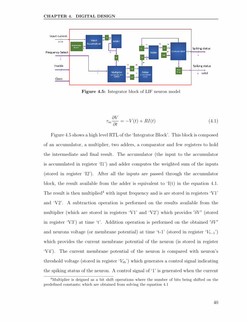
4.2.2 Integrator Block
The information from the ‘Weighted Current Block’ is fed into the ‘Integrator Block’.
This block basically performs integration of current (based on equation 4.1) being fed
in from the ‘Weighted Current Block’ until a threshold value is reached and outputs
the spiking status (indicates whether the neuron is currently spiking or not). Once
a threshold value is reached, the integrator is reset (i.e. the membrane potential is
set to resting potential) and a control signal triggering the spike (i.e enabling ‘Spike
Generator Block’) is generated.
The integration of input current is based on the LIF neuron model which can be
mathematically modeled as in equation 4.1; where τm is the time constant (R*C),
V(t) is voltage (or membrane potential) at time t, I(t) is the input current at time t.
3Where ‘n’ is number of neurons in the liquid layer + number of inputs from the pre-processinglayer to the liquid.
39
CHAPTER 4. DIGITAL DESIGN
Figure 4.5: Integrator block of LIF neuron model
τm∂V
∂t= −V (t) +RI(t) (4.1)
Figure 4.5 shows a high level RTL of the ‘Integrator Block’. This block is composed
of an accumulator, a multiplier, two adders, a comparator and few registers to hold
the intermediate and final result. The accumulator (the input to the accumulator
is accumulated in register ‘I1’) and adder computes the weighted sum of the inputs
(stored in register ‘I2’). After all the inputs are passed through the accumulator
block, the result available from the adder is equivalent to ‘I(t) in the equation 4.1.
The result is then multiplied4 with input frequency and is are stored in registers ‘V1’
and ‘V2’. A subtraction operation is performed on the results available from the
multiplier (which are stored in registers ‘V1’ and ‘V2’) which provides ′δV ′ (stored
in register ‘V3’) at time ‘t’. Addition operation is performed on the obtained ′δV ′
and neurons voltage (or membrane potential) at time ‘t-1’ (stored in register ‘Vt−1’)
which provides the current membrane potential of the neuron (is stored in register
‘V4’). The current membrane potential of the neuron is compared with neuron’s
threshold voltage (stored in register ‘Vth’) which generates a control signal indicating
the spiking status of the neuron. A control signal of ‘1’ is generated when the current
4Multiplier is deigned as a bit shift operations where the number of bits being shifted on thepredefined constants; which are obtained from solving the equation 4.1
40

CHAPTER 4. DIGITAL DESIGN
membrane potential of the neuron is greater than or equal to that of the neuron’s
threshold voltage, else a control signal of ‘0’ is generated.
4.2.3 Spike Generator Block
The basic functionality of this block is to generate a spike when triggered by the
‘Integration Block’. A control signal from the ‘Integration Block’ enables this ‘Spike
Generator Block’. Once enabled this takes control over the spiking status register
of the neuron and resets it after one complete spike duration. When the block is
already in an enabled state and is currently spiking any further enable input from
the integrator block enters the queue until the neuron completes spiking. Then the
‘Spike Generator Block’ is re-enabled. The queue has the capacity to hold one spike
enable signal.
A new spike generator model is used in this design resulting in a huge optimization
of hardware resources and there by power reduction. The spike generator used in this
model can be mathematically represented as in equation 4.2, where a predefined
value is chosen based on the maximum/peak spike value required. This equation
also eliminates the need for a refractory period, as the generated spike exploits this
behavior (can be observed by the graphical representation the equation 4.2). ISpiket
is the spike value generated by the ‘Spike Generator Block’ at time ‘t’ and the constant
2−3 is chosen after careful analysis thereby generating a spike and at the same time
replacing the multiplier.
ISpiket =
ISpiket−1 − (2−3) ∗ ISpiket−1 if t > 1
Predefined Constant if t = 1
(4.2)
Figure 4.6 shows a high level RTL of this block, designed to perform the math-
ematical operation as in equation 4.2. It can be inferred from figure 4.6 that this
block is composed of an accumulator, adder, comparator, a bit shift operator and
41

CHAPTER 4. DIGITAL DESIGN
Figure 4.6: Spike generator block of LIF neuron model
four 12-bit, one 6-bit and one 1-bit registers to hold the intermediate and final result.
4.2.4 Spike Counter Block
The basic functionality of this block is to keep track of the number of spikes that
occurred during each window duration. At the end of each scanning window duration
the spike count (number of spikes that occur during the current window duration) is
fed into the output layer from each neuron. This block is designed to self-reset and
all the blocks including the Finite State Machine (FSM) in the neuron block after
every scanning window duration.
4.3 Output Layer
As discussed in section 3.1.6 the software model of output layer is a two layer MLP.
For hardware optimizations, only the last layer weights are updated i.e. the output
layer is implemented as an ELM. The number of neurons in the input layer, hidden
layer and output layer are chosen to be 6, 4 and 1 respectively. Further increase in
the number of neurons doesn’t show any significant performance improvement.
Figure 4.7 shows a high level RTL of this block. All the inputs variables (i.e.
spike counts) and intermediate results in the output layer are registered. Weights are
stored in distributed RAM using single bit precision in floating point representation
42

CHAPTER 4. DIGITAL DESIGN
Figure 4.7: Output layer of LSM
Figure 4.8: IEEE754 Single precision 32-bit
(i.e. 1 bit for sign, 8 bits to represent the exponent and 24 bits to represent the
fraction as shown in figure 4.8) following ‘IEEE754 Single precision 32-bit’ standard.
The results i.e. spike counts obtained from the liquid are fed into the output
layer along with an enable signal indicating the input is ready for processing. Input
‘TrainBool’ indicated the network to train the weights during training phase and not
to update during the testing phase (‘TrainBool’ = ‘1’ for training; ‘TrainBool’ = ‘0’
for testing) and the label (or the class) is indicated by input ‘Target’ during training
phase which is otherwise ignored.
43

CHAPTER 4. DIGITAL DESIGN
Figure 4.9: Input to output comparison between sigmoid and piece-wise sigmoid functions
Y =
1 if |x| ≥ 5
0.03125 ∗ |x|+ 0.84375 if 2.375 ≤ |x| ≤ 5
0.125 ∗ |x|+ 0.625 if 1 ≤ |x| ≤ 2.375
0.25 ∗ |x|+ 0.5 if 0 ≤ |x| ≤ 1
1− Y if x ≤ 0
(4.3)
All the neurons in the output layer follow linear activation function except for that
neuron in the last layer which follows sigmoid activation function. Sigmoid activation
function is designed using piece-wise approximation model instead of using look-up
tables. This design choice saves the total number of memory elements significantly.
A look-up table if implemented using RAM will act as a bottleneck of the design
thereby inhibiting the design’s real-time processing capability. When a Look-up table
is implemented using registers it requires 1000’s of 32 bit registers. Where as a
44

CHAPTER 4. DIGITAL DESIGN
piece-wise approximation model requires no registers but does require only a 32 bit
floating point adder. The piece-wise approximation model used in this design can
me mathematically represented as 4.3 and is presented in [43]. Figure 4.9 shows the
difference in results for sigmoid activation function neuron with respect to piece-wise
sigmoid activation function. It can be observed here that the behavior of both the
models is almost identical to each other where as the hardware resource requirement
is drastically different. This design approach of sigmoid activation function helps in
resource optimization there by resulting in area and power optimizations.
4.4 Summary
in this chapter a fully digital design approach towards modeling an LSM is presented.
A bottom up hierarchical approach is followed to implement the liquid layer, the main
block of the LSM.
45

Chapter 5
Spatio-temporal Datasets
Matlab is used as a simulation platform to build the behavioral model of the proposed
network (refer chapter 3). An exhaustive parameter sweep of several parameters were
done on this behavioral model and the results are analyzed to build a hardware
efficient design. The model includes managing the dataset, preprocessing, input,
liquid and output layer of LSM and a post-processing block to compute the accuracy.
The behavioral model remains the same over different applications/datasets except for
the preprocessing and output layer of LSM which are application dependent. Using
this approach the systems are analyzed in detail to find the appropriate parameters to
enhance the accuracy. The datasets used are presented in section 5.1 and the results
are presented and analyzed in chapter 6.
5.1 Data Sets
The proposed model is tested on two different datasets which are spatio-temporal in
nature. The two datasets are chosen to demonstrate that the proposed design is not
application specific and can be used for various applications involving spatio-temporal
signal.
46

CHAPTER 5. SPATIO-TEMPORAL DATASETS
5.1.1 Epilepsy
The EEG dataset used was presented in [1]. Signals in this dataset were recorded
using a 128-channel amplifier system. A 12 bit analog-to-digital converter is used
to sample the signals at a rate of 173.61 samples per second, with a total of 500
single-channel EEG segments.
The dataset is divided into five sets A-E, each set contains 100 EEG segments
of 23.6 seconds each. These segments were selected and cut from multichannel EEG
records after visual inspection for artifacts. Set A and E of this dataset are used
in this work. Set A contains EEG recordings of five healthy volunteers in a relaxed
state. Surface electrodes, as shown in figure 5.1a, are used to collect the data. The
signals were collected from all these electrodes where each segment contains data
of one electrode. Set E contains seizure activity segments taken from five epilepsy
patients during presurgical evaluation. Depth electrodes implanted symmetrically
into the hippocampal formations of the brain are used to collect the data(figure
5.1b). Figures 5.2a and 5.2b show EEG signal samples of normal and seizure cases
respectively.
5.1.2 User Verification Using Biometric Walking Pattern
Biometrics are biological features of an individual that offer unique descriptors. These
are used in applications such as user identification and security. For the user veri-
fication using biometric walking pattern dataset, there are very few datasets that
are freely available. One such example is user identification based on their walking
pattern or gait [17]. In this dataset, the walking patterns of 22 individuals were mea-
sured using an android smart phone in a chest shirt pocket. The smart phone used
androids accelerometer at the highest sampling frequency to record the motion of the
individual which is 33 samples per second. Each person was required to walk along
an identified path but no restrictions were imposed on how they walk. The accelera-
47

CHAPTER 5. SPATIO-TEMPORAL DATASETS
(a) Scheme of the locations of surface elec-trodes according to the international 10-20system which is used to collect EEG signalsfor set A.
(b) Scheme of intracranial electrodes im-planted for presurgical evaluation of epilepsypatients which is used to collect EEG signalsfor set E.
Figure 5.1: Electrode placements [1].
(a) EEG Sample data for Normal Subject
(b) EEG Sample Data for seizure
Figure 5.2: Time series EEG signal samples for (a) Normal case (dataset A) and (b)Seizure case (dataset E).
48

CHAPTER 5. SPATIO-TEMPORAL DATASETS
tion in the x, y, and z directions was recorded for each individual until the path was
completed. This data set was used to train the network to identify/authorize two
subjects. A sample of the accelerometer measurements in each direction are shown
in Fig. 5.3.
(a) Acceleration in X-direction for two individuals.
(b) Acceleration in Y-direction for two individuals.
(c) Acceleration in Z-direction for two individuals.
Figure 5.3: Accelerometer Recordings in XYZ Coordinates for two individuals.
49

CHAPTER 5. SPATIO-TEMPORAL DATASETS
5.2 Summary
Two data sets discussed in this chapter are used to benchmark the LSM design. The
EEG signals are used for epileptic seizures detection, which has several medical ap-
plications. Data recorded from an accelerometer sensor is used for user identification
based on walking patterns.
50
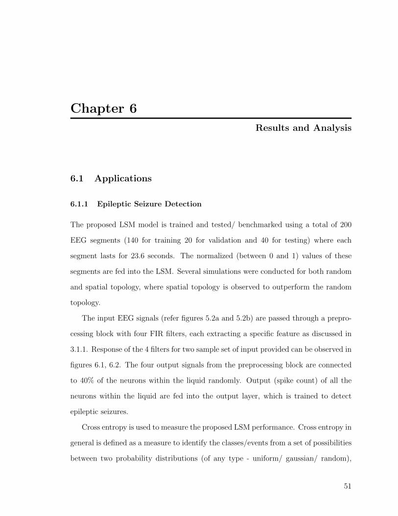
Chapter 6
Results and Analysis
6.1 Applications
6.1.1 Epileptic Seizure Detection
The proposed LSM model is trained and tested/ benchmarked using a total of 200
EEG segments (140 for training 20 for validation and 40 for testing) where each
segment lasts for 23.6 seconds. The normalized (between 0 and 1) values of these
segments are fed into the LSM. Several simulations were conducted for both random
and spatial topology, where spatial topology is observed to outperform the random
topology.
The input EEG signals (refer figures 5.2a and 5.2b) are passed through a prepro-
cessing block with four FIR filters, each extracting a specific feature as discussed in
3.1.1. Response of the 4 filters for two sample set of input provided can be observed in
figures 6.1, 6.2. The four output signals from the preprocessing block are connected
to 40% of the neurons within the liquid randomly. Output (spike count) of all the
neurons within the liquid are fed into the output layer, which is trained to detect
epileptic seizures.
Cross entropy is used to measure the proposed LSM performance. Cross entropy in
general is defined as a measure to identify the classes/events from a set of possibilities
between two probability distributions (of any type - uniform/ gaussian/ random),
51

CHAPTER 6. RESULTS AND ANALYSIS
Figure 6.1: Response of the 4 FIR filters in the input layer for the EEG signals as presentedin figure 5.2a.
Figure 6.2: Response of the 4 FIR filters in the input layer for the EEG signals as presentedin figure 5.2b.
52

CHAPTER 6. RESULTS AND ANALYSIS
Figure 6.3: Liquid response for EEG signals.
Figure 6.4: Liquid response for EEG signals.
53

CHAPTER 6. RESULTS AND ANALYSIS
especially used when the probability distributions of the classes/events are unknown.
Cross entropy defines the loss function in machine learning. It arises as a natural cost
function for a network consisting of non linear activation functions such as sigmoid or
softmax and used to maximize the likelihood of classifying the input data to improve
the prediction accuracy. Figure 6.51 shows the performance of the liquid in terms of
cross-entropy of output layer over epochs for the proposed behavioral model. It can
be observed that there is a gradual decrease in cross entropy as the number of epochs
increases, this indicates the decrease in error (i.e. increase in prediction accuracy).
Figure 6.6 shows the confusion matrix obtained as a result of predictions from LSM; an
accuracy of 85.5% , 84.3% and 84.2% for training, validation and testing are observed
respectively for the proposed behavioral model and a test accuracy of ∼78.65% for
hardware model2.
There are existing models that are proposed for epileptic seizure detection on var-
ious data sets. As presented in [44], a multi-wavelet transform based approximate
entropy and artificial neural networks were used for epilepsy detection but the prepro-
cessing methods that were used to remove artifacts restricts the design in real time
predictions3. Also the design uses entropy of the data during preprocessing, which
makes it highly application specific. It will be inefficient for other artifacts that do
occur and are not present in the data set. Similarly designs proposed in [45], [46] and
[47] lack real time prediction capability. Also the models presented in [48] and [49]
use frequency domain analysis, which restricts its use for real time seizure detection.
To summarize, existing models use preprocessing/ analysis inhibiting the model from
real time seizure detection. Secondly, these designs are application specific. The pro-
1The dotted line’s along x and y axis in the figure points to the lowest cross entropy over theruns/epochs during training.
2This decrease in performance is observed as a result of hardware optimizations in the outputlayer of the LSM; where as the performance of the liquid (or reservoir) is observed to be same asthat of the behavioral/ software model.
3Real time design refers to processing inputs dynamically without the use of additional storageto buffer the inputs (in a 1sec time interval). Existing designs have the processing time rangingup-to 20 seconds, where as short time seizures last only for 5/6 seconds
54

CHAPTER 6. RESULTS AND ANALYSIS
Figure 6.5: Cross-Entropy vs Epochs for epileptic seizure detection.
Figure 6.6: Confusion matrix based on the predictions made by the LSM for epilepticseizure detection.
55
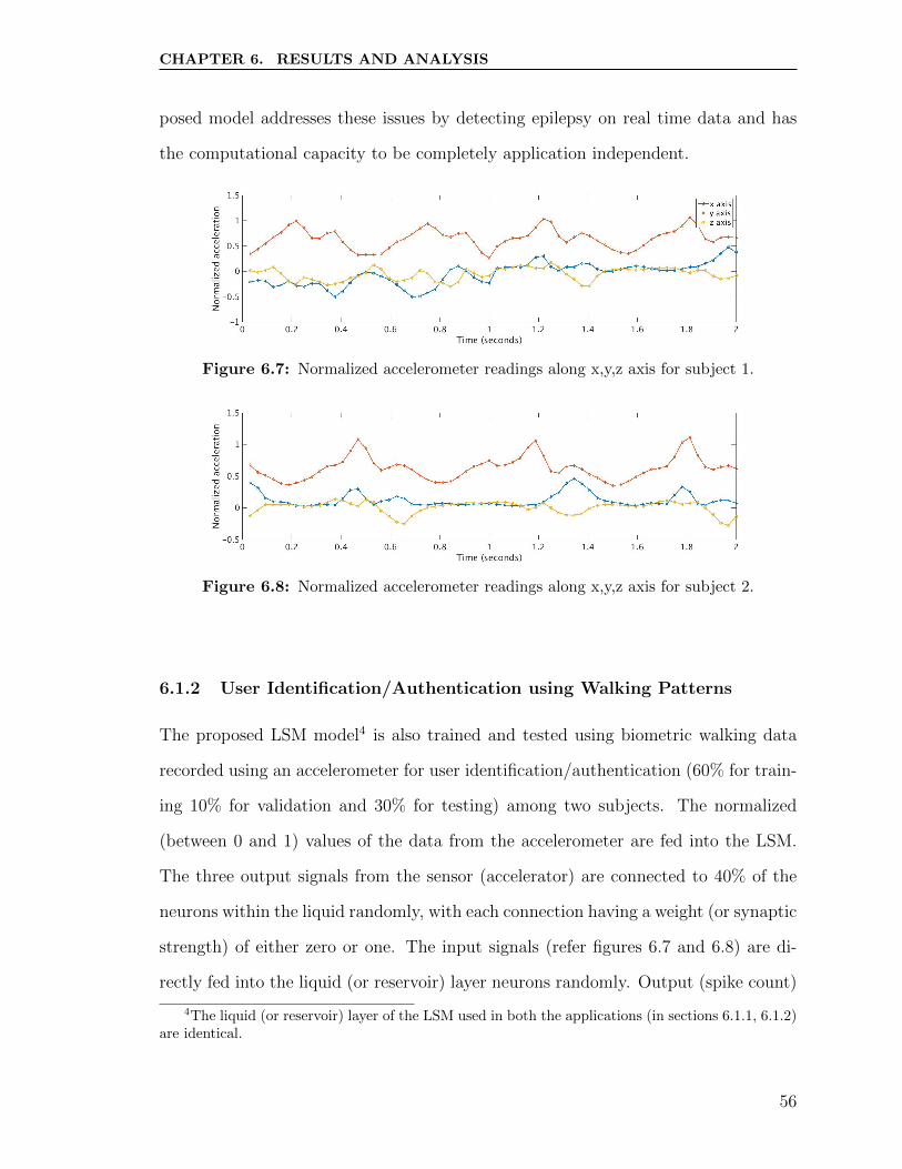
CHAPTER 6. RESULTS AND ANALYSIS
posed model addresses these issues by detecting epilepsy on real time data and has
the computational capacity to be completely application independent.
Figure 6.7: Normalized accelerometer readings along x,y,z axis for subject 1.
Figure 6.8: Normalized accelerometer readings along x,y,z axis for subject 2.
6.1.2 User Identification/Authentication using Walking Patterns
The proposed LSM model4 is also trained and tested using biometric walking data
recorded using an accelerometer for user identification/authentication (60% for train-
ing 10% for validation and 30% for testing) among two subjects. The normalized
(between 0 and 1) values of the data from the accelerometer are fed into the LSM.
The three output signals from the sensor (accelerator) are connected to 40% of the
neurons within the liquid randomly, with each connection having a weight (or synaptic
strength) of either zero or one. The input signals (refer figures 6.7 and 6.8) are di-
rectly fed into the liquid (or reservoir) layer neurons randomly. Output (spike count)
4The liquid (or reservoir) layer of the LSM used in both the applications (in sections 6.1.1, 6.1.2)are identical.
56

CHAPTER 6. RESULTS AND ANALYSIS
Figure 6.9: Cross-Entropy vs Epochs for user identification/authentication.
of all the neurons within the liquid are connected to the output layer, which is trained
to detect the user.
Figure 6.10: Confusion matrix based on the predictions made by the LSM for user iden-tification/authentication.
Figure 6.9 shows the performance of the liquid in terms of cross-entropy of output
layer over number of epochs for user identification/authentication. As the number of
57

CHAPTER 6. RESULTS AND ANALYSIS
epochs increases it can be observed that there is a gradual decrease in cross entropy
which indicates the decrease in error (i.e. increase in prediction accuracy). This is
as a result of output layer leaning to classify the results provided by the reservoir
and from its respective miss-classifications. Figure 6.10 shows the confusion matrix
obtained as a result of predictions from LSM. An average accuracy of 99.7% , 98% and
98.65% for training, validation and testing is observed respectively, for the proposed
behavioral model over 50 independent trials5.
6.2 Reservoir Metrics
The performance of the liquid depends on various factors like the pseudo-randomly
generated weights, number of neurons and neuron type (inhibitory, excitatory). These
factors affect the overall performance of the system. As the goal of LSM is to build a
liquid independent of an application, there is a need for generic metrics that evaluate
the performance of the liquid. Several metrics have been proposed in the literature
[50], [51] and [52], which compared the ability of reservoir metrics to measure the
performance of several reservoir topologies. The reservoir metrics used are: kernel
quality, class separation and Lyapunov’s exponent. Results show that kernel quality
and Lyapunov’s exponent strongly correlate with reservoir performance.
6.2.1 Kernel quality
Kernel quality is a measure of the linear separability of the reservoir [50]. In this
metric, the reservoir response for all the sets of inputs are used. The rank of the result
matrix indicates the kernel quality of the liquid. The rank of the matrix determines
the correlation between neurons within the liquid. If the rank of the matrix equals the
number of neurons within the liquid then it indicates that all the neurons generate
5It is to be noted that accuracy of 100% , 100% and 94.7% for training, validation and testingis observed respectively (shown in figure 6.10) this is for a random independent trial and not for anaverage over independent trials
58

CHAPTER 6. RESULTS AND ANALYSIS
unique response from each other. For the proposed behavioral model, a kernel quality
of 59 (i.e rank of matrix is 59) is observed for a liquid with 60 neurons; which indicates
a minute co-relation between neurons within the liquid.
6.2.2 Separation Property of the Liquid
The separation property describes how unique the state of the liquid is for different
input classes. This has a direct impact on the performance of the readout layer. An
ideal liquid should have a high inter-class variance with low intra-class variance. This
will enhance the performance of the readout layer. In order to evaluate the liquid,
equation 6.1 is used [53], which is an expanded version of the work from [54] .
Sepx(t) =Cd(t)
Cv(t) + 1(6.1)
In 6.1, the inter-class distance is represented by Cd and determined by using
equation 6.2, while the intra-class distance is represented by Cv and determined using
equation 6.3 where N represents the total number of classes, k represents the number
of samples of that class, and µ (Om(t)) represents the mean state of class m.
The separation property of the reservoir was found to be 0.1028 and 0.2945 for
the seizure detection and user identification tasks respectively. From these results
we were able to see that the intra-class variance was significantly larger than the
inter-class distance. This demonstrates the liquid’s capability of distinguishing to
different time-series signal from each other efficiently there by having a direct impact
on classification accuracy obtained from the output layer.
Cd (t) =N∑m=1
N∑n=1
||µ (Om (t))− µ (On (t)) ||N2
(6.2)
CV (t) =1
N
N∑m=1
∑ki=1 ||µ (Om(t))− xi(t)||
K(6.3)
59

CHAPTER 6. RESULTS AND ANALYSIS
Figure 6.11: Lyapunov Exponent for reservoir performance on different tasks.
6.2.3 Lyapunov Exponent
In [50], it was shown that networks like the LSM have the greatest computational
capability when operating on the edge of chaos. The Lyapunov exponent provides a
method to determine if the networks are stable or chaotic. If the number is positive,
the system is behaving chaotically and if it is negative the network is stable. This
means ideally a network should have a Lyapunov exponent value of ‘0’ which would
represent operation at the edge of chaos. The Lyapunov exponent is calculated using
equation 6.4 as explained in [55].
λ(t) = kN∑j=1
ln
(||xj(t)− xj(t)||||uj(t)− uj(t)||
)(6.4)
uj(t) and its nearest neighbor in the input space uj(t) represent the initial inputs
to the liquid. xj and xj are the respective reservoir states of the two input vectors.
K is a scalar that can be chosen based on the data. The proposed network has a
Lyapunov Exponent of 2.1154 and 1.9654 for user identification and seizure detection
respectively, as shown in figure 6.11. These values were determined by setting k equal
to 1. The positive values indicate the reservoir is slightly chaotic, which agrees with
the high intra-class variance as presented in 6.2.2.
60

CHAPTER 6. RESULTS AND ANALYSIS
Table 6.1: Area estimates of the liquid for different TSMC technology nodes.
TSMC 180 nm TSMC 65 nmTotal Area 16mm2 2mm2
6.3 Power and Area
Power dissipation of the ASIC implementation of liquid (or reservoir) for the proposed
model is analyzed. Synopsys tool is used to analyze the power consumption of the
proposed model at 180nm and 65nm technology node the results are presented in
table 6.2. Area results were also obtained using synopsys tools of the proposed model
at 180nm and 65nm technology node and are observed to be 16mm2 and 2mm2
respectively as presented in 6.1.
Table 6.2: Power consumption of the liquid at different TSMC technology node.
TSMC 180 nm TSMC 65 nmDynamic Power (mW) 371.29 55.61
Static Power (µW) 61.33 69.61Total Power (mW) 374.36 55.68
A Xilinx Vertex6 VSX315TL board is used to study the hardware resource utiliza-
tion. The VSX315TL FPGA board consists of 196,800 LUT’s. The FPGA resource
utilization of the liquid (or reservoir) is are presented in Table 6.6. The number of
occupied LUT’s is 33,654 i.e. only 16% of the Xilinx Vertex6 VSX315TL FPGA
device.
Table 6.3: Power estimates of the liquid on a Xilinx Vertex6 VSX315TL FPGA board.
On-Chip Power (mW) Used Available Utilization (%)Clock 4.21 1 - -Logic 2.65 32654 196800 17Signals 3.52 50815 - -Static Power 3336.68 - - -Total 3347.06 - - -
61

CHAPTER 6. RESULTS AND ANALYSIS
Table 6.4: Area estimates of the liquid on a Xilinx Vertex6 VSX315TL FPGA board.
Used Resources Available Resources Utilization (% )Number of Slice Registers 33,550 393,600 8Number of Slice LUTs 33,654 196,800 16Number of Occupied Slices 10,617 49,200 21Number of LUT FF pairs used 37,761 - -Number of RAMB36E1 used 65 704 9Number of RAMB18E1 used 0 1,408 0
Table 6.5: Area estimates of the Pre-processing block on a Xilinx Vertex6 VSX315TLFPGA board.
Used Resources Available Resources Utilization (% )Number of Slice Registers 812 393,600 <1Number of Slice LUTs 754 196,800 <1Number of Occupied Slices 400 49,200 <1Number of LUT FF pairs used 1397 - -Number of DSP48E1 blocks used 4 1344 <1
Table 6.6: Area estimates of the output block on a Xilinx Vertex6 VSX315TL FPGAboard.
Used Resources Available Resources Utilization (% )Number of Slice Registers 35,670 393,600 9Number of Slice LUTs 35,965 196,800 18Number of Occupied Slices 12,577 49,200 21Number of LUT FF pairs used 9,436 -
62

Chapter 7
Conclusion and Future Work
7.1 Conclusion
This thesis work proposed and designed a LSM model using a fully digital approach.
LSM is a RNN that simplifies the training algorithm with minimal weight updates
during training. The proposed model is applied to spatio-temporal classification prob-
lems (epilepsy detection and user identification). The untrained recurrent connections
within the liquid layer of an LSM are used to map the input signal/ information to a
higher dimensional space. The output of this layer is used to train the output layer
(an ELM) of the LSM using linear model. The proposed architecture uses 3D spatial
topology with LIF neurons.
The proposed model achieves an accuracy of 84% and 98.65% for epileptic seizure
detection and user identification sing walking data respectively. The quality of the
proposed LSM is analyzed using kernel quality, separation property of the liquid and
Lyapunovs exponent metrics. The power consumption and area requirement of the
proposed model are analyzed.
63

CHAPTER 7. CONCLUSION AND FUTURE WORK
7.2 Future Work
The proposed design being an application independent, low power when an ASIC
path is chosen and being capable of processing provided inputs are real time1 this
design is a right fit in portable biometric devices.
• Explore the effect of choosing other neuron models over LIF neuron
• Explore other topologies or derive a hybrid topology.
• Use emerging technologies like memristors in the output layer for faster training
capabilities.
• Stochastic Implementation of Reservoir
• Explore applications for prediction
– Process the voice commands
– Speech to Text, User Identification, Emotion Recognition
– Anomaly detection
– Pattern recognition
• Reduce hardware recourses, area and power requirements.
1Provided the sampling rate of the input signal is less than 2KHz
64

Bibliography
[1] Andrzejak, R. G, M. Lehnertz, Klaus, Florian, Rieke, D. Christoph, E. Peter, and
C. E, “Indications of nonlinear deterministic and finite-dimensional structures in
time series of brain electrical activity: Dependence on recording region and brain
state,” Physical Review E, vol. 64, no. 6, p. 061907, 2001.
[2] E. M. Izhikevich, “Which model to use for cortical spiking neurons?” IEEE
transactions on neural networks, vol. 15, no. 5, pp. 1063–1070, 2004.
[3] S. Hochreiter, Y. Bengio, P. Frasconi, and J. Schmidhuber, “Gradient flow in
recurrent nets: the difficulty of learning long-term dependencies,” 2001.
[4] H. Jaeger, “Adaptive nonlinear system identification with echo state networks,”
in Advances in neural information processing systems, 2002, pp. 593–600.
[5] W. Maass, T. Natschlager, and H. Markram, “Real-time computing without
stable states: a new framework for neural computation based on perturbations.”
Neural computation, vol. 14, pp. 2531–2560, 2002.
[6] B. J. Grzyb, E. Chinellato, G. M. Wojcik, and W. A. Kaminski, “Facial ex-
pression recognition based on liquid state machines built of alternative neuron
models,” in 2009 International Joint Conference on Neural Networks, June 2009,
pp. 1011–1017.
[7] Y. Y. Y. Zhang, P.Li, “A digital liquid state machine with biologically inspired
learning and its application to speech recognition,” IEEE Transactions on Neural
Networks and Learning Systems, vol. 26, no. 11, pp. 2635–2649, Nov 2015.
[8] D. Verstraeten, B. Schrauwen, D. Stroobandt, and J. Van Campenhout, “Iso-
lated word recognition with the liquid state machine: a case study,” Information
Processing Letters, vol. 95, no. 6, pp. 521–528, 2005.
65

BIBLIOGRAPHY
[9] B. Schrauwen and J. Van Campenhout, “Parallel hardware implementation of
a broad class of spiking neurons using serial arithmetic,” in Proceedings of the
14th European Symposium on Artificial Neural Networks. d-side publications:,
2006, pp. 623–628.
[10] D. Roggen, S. Hofmann, Y. Thoma, and D. Floreano, “Hardware spiking neural
network with run-time reconfigurable connectivity in an autonomous robot,” in
Evolvable hardware, 2003. proceedings. nasa/dod conference on. IEEE, 2003,
pp. 189–198.
[11] A. Upegui, C. A. Pena-Reyes, and E. Sanchez, “An fpga platform for on-line
topology exploration of spiking neural networks,” Microprocessors and microsys-
tems, vol. 29, no. 5, pp. 211–223, 2005.
[12] B. Girau and C. Torres-Huitzil, “Massively distributed digital implementation of
an integrate-and-fire legion network for visual scene segmentation,” Neurocom-
puting, vol. 70, no. 7, pp. 1186–1197, 2007.
[13] B. Schrauwen, M. DHaene, D. Verstraeten, and J. Van Campenhout, “Compact
hardware liquid state machines on fpga for real-time speech recognition,” Neural
Networks, vol. 21, no. 2, pp. 511–523, 2008.
[14] A. B. S. Roy and S. Hussain, “Hardware efficient, neuromorphic dendritically
enhanced readout for liquid state machines,” in 2013 IEEE Biomedical Circuits
and Systems Conference (BioCAS), Oct 2013, pp. 302–305.
[15] D. V. B. Schrauwen, M. D’Haene and J. V. Campenhout, “Compact hardware for
real-time speech recognition using a liquid state machine,” in 2007 International
Joint Conference on Neural Networks, Aug 2007, pp. 1097–1102.
66

BIBLIOGRAPHY
[16] D. Kudithipudi, Q. Saleh, C. Merkel, J. Thesing, and B. Wysocki, “Design and
analysis of a neuromemristive reservoir computing architecture for biosignal pro-
cessing,” Frontiers in neuroscience, vol. 9, 2015.
[17] P. Casale, O. Pujol, and P. Radeva, “Personalization and user verification in
wearable systems using biometric walking patterns,” Personal and Ubiquitous
Computing, vol. 16, no. 5, pp. 563–580, 2012.
[18] W. S. McCulloch and W. Pitts, “A logical calculus of the ideas immanent in
nervous activity,” The bulletin of mathematical biophysics, vol. 5, no. 4, pp.
115–133, 1943.
[19] W. Maass, G. Schnitger, and E. D. Sontag, “On the computational power of
sigmoid versus boolean threshold circuits,” in Foundations of Computer Science,
1991. Proceedings., 32nd Annual Symposium on. IEEE, 1991, pp. 767–776.
[20] W. Maass, “Networks of spiking neurons: The third generation of neural
network models,” Neural Networks, vol. 10, no. 9, pp. 1659 – 1671,
1997. [Online]. Available: http://www.sciencedirect.com/science/article/pii/
S0893608097000117
[21] M. Kearns and L. Valiant, “Cryptographic limitations on learning boolean for-
mulae and finite automata,” Journal of the ACM (JACM), vol. 41, no. 1, pp.
67–95, 1994.
[22] H. C. Tuckwell, Nonlinear and stochastic theories. Cambridge University Press,
1988, vol. 2.
[23] M. Lukoeviius and H. Jaeger, “Reservoir computing approaches to recurrent
neural network training,” Computer Science Review, vol. 3, no. 3, pp. 127 –
149, 2009. [Online]. Available: http://www.sciencedirect.com/science/article/
pii/S1574013709000173
67

BIBLIOGRAPHY
[24] H. Jaeger, “The echo state approach to analysing and training recurrent neural
networks-with an erratum note,” p. 34, 2001.
[25] M. Tsodyks, K. Pawelzik, and H. Markram, “Neural networks with dynamic
synapses,” Neural computation, vol. 10, no. 4, pp. 821–835, 1998.
[26] P. J. Copple, “The treatment of epilepsy: Principles and practices,” Archives of
Pediatrics & Adolescent Medicine, vol. 148, no. 7, p. 769, 1994.
[27] L. Rragami, M. Gifford, and N. Edwards, “Dsv-questions remain,” Biometric
Technology Today, vol. 11, no. 11, p. 7, 2003.
[28] L. Sang, Z. Wu, and Y. Yang, “Speaker recognition system in multi-channel en-
vironment,” in Systems, Man and Cybernetics, 2003. IEEE International Con-
ference on, vol. 4. IEEE, 2003, pp. 3116–3121.
[29] H. Ailisto, V. Haataja, V. Kyllonen, and M. Lindholm, “Wearable context aware
terminal for maintenance personnel,” in European Symposium on Ambient Intel-
ligence. Springer, 2003, pp. 149–159.
[30] P. J. Denning and R. M. Metcalfe, Beyond calculation: The next fifty years of
computing. Springer Science & Business Media, 1998.
[31] L. Bianchi, D. Angelini, and F. Lacquaniti, “Individual characteristics of human
walking mechanics,” Pflugers Archiv, vol. 436, no. 3, pp. 343–356, 1998.
[32] B. Schrauwen, M. D’Haene, D. Verstraeten, and J. V. Campenhout, “Compact
hardware for real-time speech recognition using a liquid state machine,” in 2007
International Joint Conference on Neural Networks, Aug 2007, pp. 1097–1102.
[33] A. B. S. Roy and S. Hussain, “Hardware efficient, neuromorphic dendritically
enhanced readout for liquid state machines,” in 2013 IEEE Biomedical Circuits
and Systems Conference (BioCAS), Oct 2013, pp. 302–305.
68

BIBLIOGRAPHY
[34] V. Nigam and D. Graupe, “A neural-network-based detection of epilepsy,” NEU-
ROLOGICAL RESEARCH, vol. 26, no. 1, pp. 55–60, 2004.
[35] P. Buteneers, B. Schrauwen, D. Verstraeten, and D. Stroobandt, “Real-time
epileptic seizure detection using reservoir computing,” in 4th International work-
shop on Seizure Prediction, 2009.
[36] D. Gafurov, “A survey of biometric gait recognition: Approaches, security and
challenges,” in Annual Norwegian computer science conference. Citeseer, 2007,
pp. 19–21.
[37] M. S. Nixon, T. Tan, and R. Chellappa, Human identification based on gait.
Springer Science & Business Media, 2010, vol. 4.
[38] J. Han, J. Pei, and M. Kamber, Data mining: concepts and techniques. Elsevier,
2011.
[39] N. Inc., “Introduction to Biosignal Neuro-signal, EEG and EEg artifacts,” http:
//sleepshepherd.com/wp-content/uploads/2016/02/neurosky-vs-medical-eeg.
pdf, [Online; accessed 22-May-2016].
[40] H. De Garis, N. E. Nawa, M. Hough, and M. Korkin, “Evolving an opti-
mal de/convolution function for the neural net modules of atr’s artificial brain
project,” in Neural Networks, 1999. IJCNN’99. International Joint Conference
on, vol. 1. IEEE, 1999, pp. 438–443.
[41] B. Schrauwen and J. Van Campenhout, “Bsa, a fast and accurate spike train
encoding scheme,” in Proceedings of the international joint conference on neural
networks, vol. 4, no. 4. IEEE Piscataway, NJ, 2003, pp. 2825–2830.
69

BIBLIOGRAPHY
[42] X. Liu and M. Haenggi, “Throughput analysis of fading sensor networks with reg-
ular and random topologies,” EURASIP Journal on Wireless Communications
and Networking, vol. 2005, no. 4, pp. 554–564, 2005.
[43] H. Amin, K. M. Curtis, and B. R. Hayes-Gill, “Piecewise linear approximation
applied to nonlinear function of a neural network,” IEE Proceedings - Circuits,
Devices and Systems, vol. 144, no. 6, pp. 313–317, Dec 1997.
[44] L. Guo, D. Rivero, and A. Pazos, “Epileptic seizure detection using multiwavelet
transform based approximate entropy and artificial neural networks,” Journal of
Neuroscience Methods, vol. 193, no. 1, pp. 156 – 163, 2010. [Online]. Available:
http://www.sciencedirect.com/science/article/pii/S0165027010004905
[45] N. Kannathal, M. L. Choo, U. R. Acharya, and P. Sadasivan, “Entropies for
detection of epilepsy in eeg,” Computer methods and programs in biomedicine,
vol. 80, no. 3, pp. 187–194, 2005.
[46] A. Subasi, “Eeg signal classification using wavelet feature extraction and a mix-
ture of expert model,” Expert Systems with Applications, vol. 32, no. 4, pp.
1084–1093, 2007.
[47] L. Guo, D. Rivero, J. A. Seoane, and A. Pazos, “Classification of eeg signals
using relative wavelet energy and artificial neural networks,” in Proceedings of the
first ACM/SIGEVO Summit on Genetic and Evolutionary Computation. ACM,
2009, pp. 177–184.
[48] V. Srinivasan, C. Eswaran, Sriraam, and N, “Artificial neural network based
epileptic detection using time-domain and frequency-domain features,” Journal
of Medical Systems, vol. 29, no. 6, pp. 647–660, 2005.
70

BIBLIOGRAPHY
[49] A. Tzallas, M. Tsipouras, and D. Fotiadis, “Automatic seizure detection based
on time-frequency analysis and artificial neural networks,” Computational Intel-
ligence and Neuroscience, vol. 2007, 2007.
[50] R. Legenstein and W. Maass, “Edge of chaos and prediction of computational
performance for neural circuit models,” Neural Networks, vol. 20, no. 3, pp.
323–334, 2007.
[51] L. Busing, B. Schrauwen, and R. Legenstein, “Connectivity, dynamics, and mem-
ory in reservoir computing with binary and analog neurons,” Neural computation,
vol. 22, no. 5, pp. 1272–1311, 2010.
[52] J. Chrol-Cannon and Y. Jin, “On the correlation between reservoir metrics and
performance for time series classification under the influence of synaptic plastic-
ity,” PloS one, vol. 9, no. 7, p. e101792, 2014.
[53] D. Norton and D. Ventura, “Improving liquid state machines through iterative
refinement of the reservoir,” Neurocomputing, vol. 73, no. 16, pp. 2893–2904,
2010.
[54] E. Goodman and D. A. Ventura, “Spatiotemporal pattern recognition via liquid
state machines,” 2006.
[55] T. E. Gibbons, “Unifying quality metrics for reservoir networks,” in Neural Net-
works (IJCNN), The 2010 International Joint Conference on. IEEE, 2010, pp.
1–7.
71

BIBLIOGRAPHY
72