1

Scalable and Flexible Multiview MAX-VARCanonical Correlation Analysis

Xiao Fu, Member, IEEE, Kejun Huang, Member, IEEE, Mingyi Hong, Member, IEEENicholas D. Sidiropoulos, Fellow, IEEE, and Anthony Man-Cho So, Senior Member, IEEE

Abstract— Generalized canonical correlation analysis (GCCA)aims at finding latent low-dimensional common structure frommultiple views (feature vectors in different domains) of thesame entities. Unlike principal component analysis (PCA) thathandles a single view, (G)CCA is able to integrate informationfrom different feature spaces. Here we focus on MAX-VARGCCA, a popular formulation which has recently gained renewedinterest in multilingual processing and speech modeling. Theclassic MAX-VAR GCCA problem can be solved optimally viaeigen-decomposition of a matrix that compounds the (whitened)correlation matrices of the views; but this solution has seriousscalability issues, and is not directly amenable to incorporat-ing pertinent structural constraints such as non-negativity andsparsity on the canonical components. We posit regularizedMAX-VAR GCCA as a non-convex optimization problem andpropose an alternating optimization (AO)-based algorithm tohandle it. Our algorithm alternates between inexact solutions of aregularized least squares subproblem and a manifold-constrainednon-convex subproblem, thereby achieving substantial memoryand computational savings. An important benefit of our designis that it can easily handle structure-promoting regularization.We show that the algorithm globally converges to a critical pointat a sublinear rate, and approaches a global optimal solution ata linear rate when no regularization is considered. Judiciouslydesigned simulations and large-scale word embedding tasks areemployed to showcase the effectiveness of the proposed algorithm.

Index terms— Canonical correlation analysis (CCA), mul-tiview CCA, MAX-VAR, word embedding, optimization, scal-ability, feature selection

I. INTRODUCTION

Canonical correlation analysis (CCA) [1] produces low-dimensional representations via finding common structure oftwo or more views corresponding to the same entities. A viewcontains high-dimensional representations of the entities in acertain feature space – e.g., the text and audio representationsof a given word can be considered as different views of thisword. CCA is able to deal with views that have different

X. Fu, K. Huang and N.D. Sidiropoulos are supported in part by NationalScience Foundation under Project NSF ECCS-1608961 and Project NSF IIS-1447788. M. Hong is supported in part by National Science Foundation underProject NSF CCF-1526078 and by the Air Force Office of Scientific Research(AFOSR) under Grant 15RT0767.

X. Fu, K. Huang and N.D. Sidiropoulos are with the Department ofElectrical and Computer Engineering, University of Minnesota, Minneapolis,MN 55455, e-mail (xfu,huang663,nikos)@umn.edu.

M. Hong is with Department of Industrial and Manufacturing SystemsEngineering, Iowa State University, Ames, Iowa 50011, (515) 294-4111,Email: mingyi@iastate.edu.

A. M.-C. So is with the Department of Systems Engineering and Engineer-ing Management, The Chinese University of Hong Kong, Shatin, N.T., HongKong, Email: manchoso@se.cuhk.edu.hk

Engl

ish

Span

ish

Fren

ch

features features features

The same entity (“car”)

voiturecar coche

GCCA

Low-dimensional representations of the entities

entit

ies

entit

ies

entit

ies

Fig. 1. Word embedding seeks low-dimensional representations of the entities(words) that are well-aligned with human judgment. Different language data(i.e., X1-X3) can be considered as different views / feature spaces of thesame entities.

dimensions, and this flexibility is very useful in data fusion,where one is interested in integrating information acquiredfrom different domains. Multiview analysis finds numerousapplications in signal processing and machine learning, such asblind source separation [2], [3], direction-of-arrival estimation[4], wireless channel equalization [5], regression [6], clustering[7], speech modeling and recognition [8], [9], and wordembedding [10], to name a few. Classical CCA was derivedfor the two-view case, but generalized canonical correlationanalysis (GCCA) that aims at handling more than two viewshas a long history as well [11], [12]. A typical applicationof GCCA, namely, multilingual word embedding, is shown inFig. 1. Applying GCCA to integrate multiple languages wasshown to yield better embedding results relative to single-viewanalyses such as principle component analysis (PCA) [10].

Computationally, GCCA poses interesting and challengingoptimization problems. Unlike the two-view case that admitsan algebraically simple solution (via eigen-decomposition),GCCA is in general not easily solvable. Many prior worksconsidered the GCCA problem with different cost functions[11]–[13] – see a nice summary in [14, Chapter 10]. How-ever, the proposed algorithms often can only extract a singlecanonical component and then find others through a deflationprocess, which is known to suffer from error propagation.CCA and GCCA can also pose serious scalability challenges,since they involve auto- and/or cross-correlations of differentviews and a whitening stage [15]. These procedures can easilylead to memory explosion and require a large number of flopsfor computation. They also destroy the sparsity of the data,which is usually what one relies upon to deal with large-scale

2

problems. In recent years, effort has been spent on solvingthese scalability issues, but the focus is mostly on the two-view case [15]–[17].

Among all different formulations of GCCA, there is aparticular one that admits a conceptually simple solution,the so-called MAX-VAR GCCA [11], [13], [18]. MAX-VARGCCA was first proposed in [12], and its solution amounts tofinding the ‘directions’ aligned to those exhibiting maximumvariance for a matrix aggregated from the (whitened) auto-correlations of the views. It can also be viewed as a problemof enforcing identical latent representations of different viewsas opposed to highly correlated ones, which is the moregeneral goal of (G)CCA. The merit of MAX-VAR GCCA isthat it can be solved via eigen-decomposition and finds allthe canonical components simultaneously. In practice, MAX-VAR GCCA also demonstrates promising performance invarious applications such as word embedding [10] and speechrecognition [8]. On the other hand, MAX-VAR GCCA has thesame scalability problem as the other GCCA formulations:It involves correlation matrices of different views and theirinverses, which is prohibitive to even instantiate when the datadimension is large. The work in [10] provided a pragmaticway to circumvent this difficulty: PCA was first applied toeach view to reduce the rank of the views, and then MAX-VAR GCCA was applied to the rank-truncated views. Such aprocedure significantly reduces the number of parameters forcharacterizing the views and is feasible in terms of memory.However, truncating the rank of the views is prone to infor-mation loss, and thus leads to performance degradation.

Besides the basic (G)CCA formulations, structured (G)CCA[19] that seeks canonical components with pre-specified struc-ture is often considered in applications. Sparse/group-sparseCCA has attracted particular attention, since it has the abilityof discarding outlying or irrelevant features when performingCCA [20]–[22]. In multi-lingual word embedding [10], [16],[23], for example, it is known that outlying features (“stopwords”), may exist. Gene analysis is another example [20]–[22]. Ideally, CCA seeks a few highly correlated latent compo-nents, and so it should naturally be able to identify and down-weight irrelevant features automatically. In practice, however,this ability is often impaired when correlations cannot bereliably estimated, when one only has access to relatively fewand/or very noisy samples, or when there is model mismatchdue to bad preprocessing. In those cases, performing featureselection jointly with (G)CCA is well-motivated. Some otherstructure-promoting regularizations may also be of interest:Non-negativity together with sparsity have proven helpfulin analyzing audio and video data, since non-negative CCAproduces weighted sums of video frames that are interpretable[24]; non-negative CCA has also proven useful in time seriesanalysis [25]. Effective algorithms that tackle large-scale struc-tured GCCA problems are currently missing, to the best of ourknowledge.

Contributions In this work, our goal is to provide a scalableand flexible algorithmic framework for handling the MAX-VAR GCCA problem and its variants with structure-promotingregularizers. Instead of truncating the rank of the views as in

[10], we keep the data intact and deal with the problem using atwo-block alternating optimization (AO) framework. The pro-posed algorithm alternates between a regularized least squaressubproblem and an orthogonality-constrained subproblem. Themerit of this framework is that correlation matrices of theviews never need to be explicitly instantiated, and the inversionprocedure is avoided. Consequently, the algorithm consumessignificantly less memory compared to that required by theoriginal solution using eigen-decomposition. The proposedalgorithm allows inexact solution to the subproblems, andthus per-iteration computational complexity is also light. Inaddition, it can easily handle different structure-promotingregularizers (e.g. sparsity, group sparsity and non-negativity)without increasing memory and computational costs, includingthe feature-selective regularizers that we are mainly interestedin.

The AO algorithm alternates between convex and non-convex manifold-constrained subproblems, using possibly in-exact updates for the subproblems. Under such circumstances,general convergence analysis tools cannot be directly applied,and thus the associated convergence properties are not obvious.This necessitates custom convergence analysis. We first showthat the proposed algorithm globally converges to a Karush-Kuhn-Tucker (KKT) point of the formulated problem, evenwhen a variety of regularizers are employed. We also showthat the optimality gap shrinks to at most O(1/r) after riterations – i.e., at least a sublinear convergence rate canbe guaranteed. In addition, we show that when the classicMAX-VAR problem without regularization (or with a minimalenergy regularization) is considered, the proposed algorithmapproaches a global optimal solution and enjoys a linearconvergence rate.

The proposed algorithm is applied to judiciously designedsimulated data, as well as a real large-scale word embeddingproblem, and promising results are observed.

A conference version of this work appears at ICASSP 2017,New Orleans, USA, Mar. 2017 [26]. This journal versionincludes detailed convergence analysis and proofs, compre-hensive simulations, and a set of experiments using real large-scale multilingual data.Notation We use X and x to denote a matrix and a vector,respectively. X(m, :) and X(:, n) denote the mth row and thenth column of X , respectively; in particular, X(:, n1 : n2)(X(n1 : n2, :)) denotes a submatrix of X consisting of then1-n2th columns (rows) of X (MATLAB notation). ‖X‖F and‖X‖p for p ≥ 1 denote the Frobenius norm and the matrix-induced p-norm, respectively. ‖X‖p,1 =

∑mi=1 ‖X(i, :)‖p for

p ≥ 1 denotes the `p/`1-mixed norm of X ∈ Rm×n. Thesuperscripts “T ”, “†”, and “−1” denote the matrix operatorsof transpose, pseudo-inverse and inverse, respectively. Theoperator 〈X,Y 〉 denotes the inner product of X and Y .1+(X) denotes the element-wise indicator function of thenonnegative orthant – i.e., 1+(X) = +∞ if any element ofX is negative and 1+(X) = 0 otherwise.

II. BACKGROUND

Consider a scenario where L entities have different repre-sentations in I views. Let Xi ∈ RL×Mi denote the ith view

3

with its `th row Xi(`, :) being a feature vector that definesthe `th data point (entity) in the ith view (cf. Fig. 1), whereMi is the dimension of the ith feature space. The classic two-view CCA aims at finding common structure of the views vialinear transformation. Specifically, the corresponding problemcan be expressed in the following form [1]:

minQ1,Q2

‖X1Q1 −X2Q2‖2F (1a)

s.t. QTi

(XTi Xi

)Qi = I, i = 1, 2, (1b)

where the columns of Qi ∈ RMi×K correspond to theK canonical components of view Xi, and K is usuallysmall (i.e., K � min{Mi, L}). Note that we are essentiallymaximizing the trace of the estimated cross-correlations be-tween the reduced-dimension views, i.e., Tr(QT

2 XT2 X1Q1)

subject to the normalization in (1b) – which motivates theterminology “correlation analysis”. Problem (1) can be solvedvia a generalized eigen-decomposition, but this simple solutiononly applies to the two-view case. To analyze the case withmore than two views, one natural thought is to extend theformulation in (1) to a pairwise matching cirterion, i.e.,∑I−1i=1

∑Ij=i+1 ‖XiQi −XjQj‖2F with orthogonality con-

straints on XiQi for all i, where I is the number of views.Such an extension leads to the so-called sum-of-correlations(SUMCOR) generalized CCA [11], which has been shown tobe NP-hard [27]. Notice that designing efficient and scalablealgorithms for SUMCOR is an interesting topic and it startedattracting attention recently [27]–[29]. Another formulation ofGCCA is more tractable: Instead of forcing pairwise similarityof the reduced-dimension views, one can seek a common latentrepresentation of different views, i.e., [8], [10], [11], [13], [18]

min{Qi}Ii=1,G

I∑i=1

(1/2) ‖XiQi −G‖2F ,

s.t. GTG = I,

(2)

where G ∈ RL×K is a common latent representation ofthe different views. Problems (2) also finds highly correlatedreduced-dimension views as SUMCOR does. The upshot ofProblem (2) is that it “transfers” the multiple difficult con-straints QT

i XTi XiQi = I to a single constraint GTG = I ,

and thus admits a conceptually simple algebraic solution,which, as we will show, has the potential to be scaled upto deal with very large problems. In this work, we will focuson Problem (2) and its variants.

Problem (2) is referred to as the MAX-VAR formulation ofGCCA since the optimal solution amounts to taking principaleigenvectors of a matrix aggregated from the correlation ma-trices of the views. To explain, let us first assume that Xi hasfull column rank and solve (2) with respect to (w.r.t.) Qi, i.e.,Qi = X†iG, where X†i = (XT

i Xi)−1XT

i . By substitutingit back to (2), we see that an optimal solution Gopt can beobtained via solving the following:

Gopt = arg maxGTG=I

Tr

(GT

(I∑i=1

XiX†i

)G

). (3)

Let M =∑Ii=1 XiX

†i . Then, an optimal solution is Gopt =

UM (:, 1 : K), i.e., the first K principal eigenvectors of M

[30]. Although Problem (2) admits a seemingly easy solution,implementing it in practice has two major challenges:

1) Scalability Issues: Implementing the eigen-decompositionbased solution for large-scale data is prohibitive. As men-tioned, instantiating M =

∑Ii=1 Xi(X

Ti Xi)

−1XTi is not

doable when L and Mi’s are large. The matrix M is an L×Lmatrix. In applications like word embedding, L and Mi arethe vocabulary size of a language and the number of featuresdefining the terms, respectively, which can both easily exceed100, 000. This means that the memory for simply instantiatingM or (XT

i Xi)−1 can reach 75GB. In addition, even if the

views Xi are sparse, computing (XTi Xi)

−1 will create largedense matrices and make it difficult to exploit sparsity inthe subsequent processing. To circumvent these difficulties,Rastogi et al. [10] proposed to first apply the singular valuedecomposition (SVD) to the views, i.e., svd(Xi) = UiΣiV

Ti ,

and then let Xi = Ui(:, 1 : P )Σi(1 : P, 1 : P )(Vi(:, 1 :P ))T ≈ Xi, where P is much smaller than Mi and L. Thisprocedure enables one to represent the views with significantlyfewer parameters, i.e., (L + Mi + 1)P compared to LMi,and allows the original eigen-decomposition based solution toMAX-VAR GCCA to be applied; see more details in [10]. Thedrawback, however, is also evident: The procedure truncatesthe rank of the views significantly (since in practice the viewsalmost always have full column-rank, i.e., rank(Xi) = Mi),and rank-truncation is prone to information losses. Therefore,it is much more appealing to deal with the intact views.2) Structure-Promoting: Another aspect that is under-addressed by existing approaches is how to incorporate reg-ularizations on Qi to multiview large-scale CCA. Note thatfinding structured Qi is well-motivated in practice. Takingmultilingual word embedding as an example, Xi(:, n) repre-sents the nth feature in language i, which is usually defined bythe co-occurrence frequency of the words and feature n (alsoa word in language i). However, many features of Xi may notbe informative (e.g., “the” and “a” in English) or not correlatedto data in Xj . These irrelevant or outlying features couldresult in unsatisfactory performance of GCCA if not taken intoaccount. Under such scenarios, a more appealing formulationmay include a row-sparsity promoting regularization on Qi

so that some columns corresponding to the irrelevant featuresin Xi can be discounted/downweighted when seeking Qi.Sparse (G)CCA is desired in a variety of applications suchas gene analytics and fMRI prediction [20]–[22], [31], [32].Other structure such as nonnegativity of Qi was also shownuseful in data analytics for maintaining interpretability andenhancing performance; see [24], [25].

III. PROPOSED ALGORITHM

In this work, we consider a scalable and flexible algorithmicframework for handling MAX-VAR GCCA and its variantswith structure-promoting regularizers on Qi. We aim at offer-ing simple solutions that are memory-efficient, admit light per-iteration complexity, and feature good convergence propertiesunder certain mild conditions. Specifically, we consider the

4

following formulation:

min{Qi},G

I∑i=1

(1/2) ‖XiQi −G‖2F +

I∑i=1

hi (Qi) ,

s.t. GTG = I,

(4)

where hi(·) is a regularizer that imposes a certain structure onQi. Popular regularizers include

hi(Qi) = µi/2 · ‖Qi‖2F , (5a)hi(Qi) = µi · ‖Qi‖2,1, (5b)hi(Qi) = µi · ‖Qi‖1,1, (5c)

hi(Qi) = µi/2 · ‖Qi‖2F + βi · ‖Qi‖2,1, (5d)

hi(Qi) = µi/2 · ‖Qi‖2F + βi · ‖Qi‖1,1, (5e)hi(Qi) = 1+(Qi), (5f)

where µi, βi ≥ 0 are regularization parameters for balancingthe least squares fitting term and the regularization terms.The first regularizer is commonly used for controlling theenergy of the dimension-reducing matrix Qi, which also hasan effect of improving the conditioning of the subproblemw.r.t. Qi. hi(Qi) = µi‖Qi‖2,1 that we are mainly interestedin has the ability of promoting rows of Qi to be zeros (orapproximately zeros), and thus can suppress the impact of thecorresponding columns (features) in Xi – which is effectivelyfeature selection. The function hi(Qi) = µi‖Qi‖1,1 also doesfeature selection, but different columns of the dimension-reduced data, i.e., XiQi, may use different features. The reg-ularizers in (5d)-(5e) are sometimes referred to as the elasticnet regularizers in statistics, which improve conditioning of theQi-subproblem and perform feature selection at the same time.hi(Qi) = 1+(Qi) is for restraining the canonical componentsto be non-negative so that XiQi maintains interpretability insome applications like video analysis – where the columns ofXiQi are weighted combinations of time frames [25]; jointnonnegativity and sparsity regularizers can also be considered[24]. In this section, we propose an algorithm that can dealwith the regularized and the original versions of MAX-VARGCCA under a unified framework.

A. Alternating Optimization

To deal with Problem (4), our approach is founded onalternating optimization (AO); i.e., we solve two subproblemsw.r.t. {Qi} and G, respectively. As will be seen, such a simplestrategy will lead to highly scalable algorithms in terms of bothmemory and computational cost.

To begin with, let us assume that after r iterations thecurrent iterate is (Q(r),G(r)) where Q = [QT

1 , . . . ,QTI ]T

and consider the subproblem

minQi

(1/2)∥∥∥XiQi −G(r)

∥∥∥2

F+ hi(Qi), ∀i. (6)

The above problem is a regularized least squares problem.When Xi is large and sparse, many efficient algorithms canbe considered to solve it. For example, the alternating directionmethod of multipliers (ADMM) [33] is frequently employed tohandle Problem (6) in a scalable manner. However, ADMM

is a primal-dual method that does not guarantee monotonicdecrease of the objective value, which will prove useful inlater convergence analysis. Hence, we propose to employ theproximal gradient (PG) method for handling Problem (6). Toexplain, let us denote Q

(r,t)i as the tth update of Qi when

G(r) is fixed. Under this notation, we have Q(r,0)i = Q

(r)i and

Q(r,T )i = Q

(r+1)i . Let us rewrite (6) as

minQi

fi

(Qi,G

(r))

+ gi(Qi), (7)

where we define fi(Qi,G(r)) and gi(Qi) as the con-

tinuously differentiable part and the non-smooth part ofthe objective function in (6), respectively. We also define∇Qifi(Qi,G

(r)i ) as the partial derivative of the differentiable

part w.r.t. Qi. When “single-component” regularizers such ashi(Qi) = ‖Qi‖2,1 are employed, we have fi

(Qi,G

(r))

=

(1/2)∥∥XiQi −G(r)

∥∥2

Fand gi(Qi) = hi(Qi); when hi(Qi)

has multiple components such as hi(Qi) = µi/2 · ‖Qi‖2F +βi ·‖Qi‖1,1, we have fi

(Qi,G

(r))

= (1/2)∥∥XiQi −G(r)

∥∥2

F+

µi/2‖Qi‖2F and gi(Qi) = βi · ‖Qi‖1,1.Per PG, we update Qi by the following rule:

Q(r,t+1)i ← proxαigi

(Q

(r,t)i − αi∇Qifi

(Q

(r,t)i ,G

(r)i

))(8)

= arg minQi

1

2

∥∥∥Qi −H(r,t)i

∥∥∥2

F+ gi(Qi)

where H(r,t)i = Q

(r,t)i − αi∇Qi

fi(Q(r,t)i ,G

(r)i ). For many

gi(·)’s, the proximity operator in (8) has closed-form orlightweight solutions [34].

For example, if one adopts gi(Qi) = µi‖Qi‖2,1, the updaterule becomes

Q(r,t)i (m, :)←

0, ‖H(r,t)i (m, :)‖2 < µi,(

1− µi

‖H(r,t)i (m,:)‖2

)‖H(r,t)

i (m, :)‖2, o.w.

For gi(Qi) = µi‖Qi‖1,1, the update rule is similar tothe above, which is known as the soft-thresholding op-erator. For gi(Qi) = 1+(Qi), the solution is simplyQ

(r,t)i = max{H(r,t)

i ,0}. An even simpler case is hi(Qi) =(µi/2)‖Qi‖2F ; for this case, the update of Qi is simplygradient descent, i.e.,

Q(r,t+1)i ← Q

(r,t)i − αi

((XT

i Xi + µiI)Q(r,t)i −XT

i G(r)),

since the Qi-subproblem in (6) does not have a non-smoothpart.

By updating Qi using the rule in (8) for T times whereT ≥ 1, we obtain Q

(r+1)i . Next, we consider solving the

subproblem w.r.t. G when fixing {Qi}Ii=1. The G-subproblemamounts to solving the following:

minGTG=I

I∑i=1

1/2∥∥∥XiQ

(r+1)i −G

∥∥∥2

F. (9)

Expanding the above and dropping the constants, we come upwith the following equivalent problem:

maxGTG=I

Tr

(GT

I∑i=1

XiQ(r+1)i /I

).

5

An optimal solution of G is the so-called Procrustes pro-jection [35], which is implemented as follows: Let R =∑Ii=1 XiQ

(r+1)i . Then, we have

G(r+1) ← URVTR ,

where URΣRVTR = svd (R, ′econ′), and svd (·, ′econ′) de-

notes the economy-size SVD that produces UR ∈ RL×K ,ΣR ∈ RK×K and V T

R ∈ RK×K . The above update isoptimal in terms of solving the subproblem. However, sincethis subproblem has multiple optimal solutions, picking anarbitrary one from the solution set results in difficulties inanalyzing some aspects of the algorithm (specifically, the rateof convergence). To overcome this issue, we propose to solvethe following

minGTG=I

I∑i=1

1

2

∥∥∥XiQ(r+1)i −G

∥∥∥2

F+ω ·

∥∥∥G−G(r)∥∥∥2

F, (10)

where ω = (1−γ)I/2γ and γ ∈ (0, 1]. Note that ω ≥ 0 and theproximal term is added to ensure that G(r+1) will not wandervery far from G(r). An optimal solution to the above is stillsimple: The only change to the original G-solution is to usethe following modified R

R = γ

I∑i=1

XiQ(r+1)i /I + (1− γ)G(r), (11)

and the other operations (e.g., the economy-size SVD) remainthe same. While the addition of the proximal term mayseem to “degrade” an optimal solution of the G-subproblem(i.e., Problem (9)) to an inexact one, this simple changehelps establish nice convergence rate properties of the overallalgorithm, as we will see.

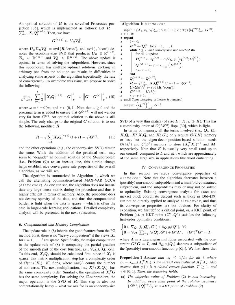
The algorithm is summarized in Algorithm 1, which wecall the alternating optimization-based MAX-VAR GCCA(AltMaxVar). As one can see, the algorithm does not instan-tiate any large dense matrix during the procedure and thus ishighly efficient in terms of memory. Also, the procedure doesnot destroy sparsity of the data, and thus the computationalburden is light when the data is sparse – which is often thecase in large-scale learning applications. Detailed complexityanalysis will be presented in the next subsection.

B. Computational and Memory Complexities

The update rule in (8) inherits the good features from the PGmethod. First, there is no “heavy computation” if the views Xi

for i = 1, . . . , I are sparse. Specifically, the major computationin the update rule of (8) is computing the partial gradientof the smooth part of the cost function, i.e., ∇Qifi(Qi,Gi).To this end, XiQi should be calculated first, since if Xi issparse, this matrix multiplication step has a complexity orderof O(nnz(Xi) · K) flops, where nnz(·) counts the numberof non-zeros. The next multiplication, i.e., XT

i (XiQi), hasthe same complexity order. Similarly, the operation of XT

i Ghas the same complexity. For solving the G-subproblem, themajor operation is the SVD of R. This step is also notcomputationally heavy – what we ask for is an economy-size

Algorithm 1: AltMaxVarinput : {Xi, µi, αi}Ii=1; γ ∈ (0, 1]; K; T ; ({Q(0)

i }Ii=1,G

(0)).1 r ← 0;2 repeat3 t← 0;4 E

(t)i ← Q

(r)i for i = 1, . . . , I;

5 while t ≤ T and convergence not reached do6 for all i, update7 H

(r,t)i ← Q

(r,t)i − αi∇Qifi

(Q

(r,t)i ;G

(r)i

);

8 Q(r,t+1)i ← proxαigi

(H

(r,t)i

);

9 t← t+ 1;10 end11 Q

(r+1)i ← Q

(r,T )i ;

12 R← γ∑Ii=1 XiQ

(r+1)i /I + (1− γ)G(r);

13 URΣRVTR ← svd (R, ′econ′);

14 G(r+1) ← URVTR ;

15 r ← r + 1;16 until Some stopping criterion is reached;

output:{Q

(r)i

}Ii=1

, G(r)

SVD of a very thin matrix (of size L×K, L� K). This hasa complexity order of O(LK2) flops [30], which is light.

In terms of memory, all the terms involved (i.e., Qi, Gi,XiQi, XT

i XiQi and XTi Gi) only require O(LK) memory

or less, but the eigen-decomposition-based solution needsO(M2

i ) and O(L2) memory to store (XTi Xi)

−1 and M ,respectively. Note that K is usually very small (and up toour control) compared to L and Mi, which are approximatelyof the same large size in applications like word embedding.

IV. CONVERGENCE PROPERTIES

In this section, we study convergence properties ofAltMaxVar. Note that the algorithm alternates between a(possibly) non-smooth subproblem and a manifold-constrainedsubproblem, and the subproblems may or may not be solvedto optimality. Existing convergence analysis for exact andinexact block coordinate descent such as those in [36]–[39]can not be directly applied to analyze AltMaxVar, and thusits convergence properties are not obvious. For clarity ofexposition, we first define a critical point, or, a KKT point, ofProblem (4). A KKT point (G∗,Q∗) satisfies the followingfirst-order optimality conditions:{

0 ∈ ∇Qi fi(Q∗i ,G

∗) + ∂Qigi(Q∗), ∀i

0 = ∇G

∑Ii=1 fi(Q

∗i ,G

∗) + G∗Λ∗, (G∗)TG∗ = I,

where Λ is a Lagrangian multiplier associated with the con-straint GTG = I , and ∂Qi

gi(Qi) denotes a subgradient ofthe (possibly) non-smooth function gi(Qi). We first show that

Proposition 1 Assume that αi ≤ 1/Li for all i, whereLi = λmax(XT

i Xi) is the largest eigenvalue of XTi Xi. Also

assume that gi(·) is a closed convex function, T ≥ 1, andγ ∈ (0, 1]. Then, the following holds:(a) The objective value of Problem (2) is non-increasing.

In addition, every limit point of the solution sequence{G(r), {Q(r)

i }}r is a KKT point of Problem (2).

6

(b) If Xi and Q(0)i for i = 1, . . . , I are bounded and

rank(Xi) = Mi, then, the whole solution sequenceconverges to the set K that consists of all the KKT points.

Proposition 1 (a) characterizes the limit points of the solu-tion sequence: Even if only one proximal gradient step isperformed in each iteration r, every convergent subsequenceof the solution sequence attains a KKT point of Problem (4).As we demonstrate in the proof (relegated to the Appendix),AltMaxVar can be viewed as an algorithm that successivelydeals with local upper bounds of the two subproblems, whichhas a similar flavor as block successive upper bound minimiza-tion (BSUM) [37]. However, the generic BSUM frameworkdoes not cover nonconvex constraints such as GTG = I ,Hence, the convergence properties of BSUM cannot be ap-plied to show Proposition 1. To fill this gap, careful customconvergence analysis is provided in the appendix. The (b) partof Proposition 1 establishes the convergence of the wholesolution sequence – which is a much stronger result. Theassumption rank(Xi) = Mi, on the other hand, is alsorelatively more restrictive.

It is also meaningful to estimate the number of iterationsthat is needed for the algorithm to reach a neighborhood of aKKT point. To this end, let us define the following potentialfunction:

Z(r+1) =

T−1∑t=0

I∑i=1

∥∥∥∇QiFi

(Q

(r,t)i ,G(r)

)∥∥∥2

F

+∥∥∥G(r) −

∑Ii=1 XiQ

(r+1)i /I + G(r+1)Λ(r+1)

∥∥∥2

F,

where Fi(Qi,G) = fi(Qi,G) + gi(Qi,G), Λ(r+1) is theLagrangian multiplier associated with the solution G(r+1), and

∇QiFi(Q

(r,t)i ,G(r)) =

1

αi

(Q

(r,t)i − proxαigi

(H

(r,t)i

)).

Note that the update w.r.t. Qi can be written asQ

(r,t+1)i = Q

(r,t)i − αi∇Qi

Fi(Q(r,t)i ,G

(r)i ) [34] – and there-

fore ∇QiFi(Q(r,t)i ,G(r)) is also called the proximal gradient

of the Qi-subproblem w.r.t. Qi at (Q(r,t)i ,G(r)), as a counter-

part of the classic gradient that is defined on smooth functions.One can see that Z(r+1) is a value that is determined bytwo consecutive outer iterates indexed by r and r + 1 of thealgorithm. Z(r+1) has the following property:

Lemma 1 Z(r+1) → 0 implies that({Q(r)

i }i,G(r))

ap-proaches a KKT point.

The proof of Lemma 1 is in Appendix B. As a result, wecan use the value of Z(r+1) to measure how close is thecurrent iterate to a KKT point, thereby estimating the iterationcomplexity. Following this rationale, we show that

Theorem 1 Assume that αi < 1/Li, 0 < γ < 1 and T ≥ 1.Let δ > 0 and J be the number of iterations when Z(r+1) ≤ δholds for the first time. Then, there exists a constant v suchthat δ ≤ v/J−1; that is, the algorithm converges to a KKTpoint at least sublinearly.

The proof of Theorem 1 is relegated to Appendix C. By The-orem 1, AltMaxVar reduces the optimality gap (measuredby the Z-function) between the current iterate and a KKTpoint to O(1/r) after r iterations. One subtle point that isworth mentioning is that the analysis in Theorem 1 holdswhen γ < 1 – which corresponds to the case where theG-subproblem in (9) is not optimally solved (to be specific,what we solve is a local surrogate in (10)). This reflectssome interesting facts in AO – when the subproblems arehandled in a more conservative way using a controlled stepsize, convergence rate may be guaranteed. On the other hand,more conservative step sizes may result in slower convergence.Hence, choosing an optimization strategy usually poses atrade-off between practical considerations such as speed andtheoretical guarantees.

Proposition 1 and Theorem 1 characterize convergenceproperties of AltMaxVar with a general regularization termhi(·). It is also interesting to consider the special case wherehi(·) = (µi/2)‖ · ‖2F – which correspond to the originalMAX-VAR formulation (when µi = 0) and its “diagonallyloaded” version (µi > 0). The corresponding problem isoptimally solvable via taking the K leading eigenvectors ofM =

∑Ii=1 Xi(X

Ti Xi + µiI)−1XT

i [10]. It is natural towonder if AltMaxVar has sacrificed optimality in dealingwith this special case for the sake of gaining scalability?The answer is – thankfully – not really. This is not entirelysurprising; to explain, let us denote U1 = UM (:, 1 : K)and U2 = UM (:,K + 1 : L) as the K principal eigen-vectors of M and the eigenvectors spanning its orthogonalcomplement, respectively. Recall that our ultimate goal is tofind G that is a basis of the range space of U1, denoted byR(U1). Hence, the speed of convergence can be measuredthrough the distance between R(G) and R(U1). To this end,we adopt the definition of subspace distance in [30], i.e.,dist

(R(G(r)),R(U1)

)= ‖UT

2 G(r)‖2 and show that

Theorem 2 Denote the eigenvalues of M ∈ RL×L byλ1, . . . , λL in descending order. Consider hi(·) = µi

2 ‖ · ‖2F

for µi ≥ 0 and let γ = 1. Assume that rank(Xi) = Mi,λK > λK+1, and R(G(0)) is not orthogonal to any compo-nent in R(U1), i.e.,

cos(θ) = minu∈R(U1),v∈R(G(0))

|uTv|(‖u‖2‖v‖2)

= σmin(UT1 G(0)) > 0.

(12)

In addition, assume that each subproblem in (6) is solved toaccuracy ε(r) at iteration r, i.e., ‖Q(r)

i −Q(r)i ‖2 ≤ ε(r), where

Q(r)i = (XT

i Xi + µiI)−1XTi G

(r−1). Assume that ε(r) issufficiently small, i.e.,

ε(r) ≤ λK − λK+1

3∑Ii=1 λmax(Xi)

(13)

×min{σmin

(UT

2 G(r)), σmax

(UT

1 G(r))}

.

Then, dist(R(G(r)),R(U1)

)approaches zero at a linear

rate; i.e.,

dist(R(G(r)),R(U1)

)≤(

2λK+1 + λK2λK + λK+1

)rtan(θ).

7

Theorem 2 ensures that if a T suffices for the Q-subproblem toobtain a good enough approximation of the solution of Prob-lem (6), the algorithm converges linearly to a global optimalsolution – this means that we have gained scalability usingAltMaxVar without losing optimality. Note that (13) meansthat the Qi-subproblem may require a higher solution accuracywhen R(G(r)) approaches R(U1), since σmin(UT

2 G(r)) isclose to zero under such circumstances. Nevertheless, sincethe result is based on worst-case analysis, the solution of theQi-subproblem can be far rougher in practice – and one canstill observe good convergence behavior of AltMaxVar. Infact, in our simulations, we observe that using T = 1 alreadygives very satisfactory results (as will be shown in the nextsection), which leads to computationally very cheap updates.

Remark 1 According to the proof of Theorem 2, when deal-ing with Problem (4) with hi(·) = µi/2‖ · ‖2F , the procedure ofAltMaxVar can be interpreted as a variant of the orthogonaliteration [30]. Based on this insight, many other approachescan be taken; e.g., the Qi-subproblem can be handled byconjugate gradient and the SVD step can be replaced by theQR decomposition – which may lead to computationally evencheaper updates. Nevertheless, our interest lies in solving (4)with a variety of regularizations under a unified framework,and the aforementioned alternatives cannot easily handle otherregularizations.

V. NUMERICAL RESULTS

In this section, we use synthetic data and real experimentsto showcase the effectiveness of the proposed algorithm.Throughout this section, the step size of the Qi-subproblemof AltMaxVar is set to be αi = 0.99 × 1/λmax(XT

i Xi).When hi(Qi) = µi/2‖Qi‖2F is employed, we let γ = 1following Theorem 2; otherwise, we let γ = 0.9999 – so thatthe convergence rate guarantee in Theorem 1 holds. All theexperiments are coded in Matlab and conducted on a Linuxserver equipped with 32 1.2GHz cores and 128GB RAM.

A. Sanity Check: Small-Size Problems

We first use small-size problem instances to verify theconvergence properties that were discussed in the last section.

1) Classic MAX-VAR GCCA: We generate the syntheticdata in the following way: First, we let Z ∈ RL×N be acommon latent factor of different views, where the entries of Zare drawn from the zero-mean i.i.d. Gaussian distribution andL ≥ N . Then, a ‘mixing matrix’ Ai ∈ RN×Mi is multipliedto Z, resulting in Yi = ZAi. We let M1 = . . . = MI = Min this section. Finally, we add noise so that Xi = Yi +σNi.Here, Ai and Ni are generated in the same way as Z.We first apply the algorithm with the regularization termhi(·) = µi/2‖ · ‖2F and let µi = 0.1. Since L and M aresmall in this subsection, we employ the optimal solution thatis based on eigen-decomposition as a baseline. The multiviewlatent semantic analysis (MVLSA) algorithm that was proposedin [10] is also employed as a baseline. In this section, we stopAltMaxVar when the absolute change of the objective valueis smaller than 10−4.

100 101 102 103

iterations

10-2

10-1

100

101

102

103

104

cost

val

ue

Proposed (T=1, warm)Proposed (T = 10, warm)Proposed (solved, warm)Proposed (T = 1,randn)Proposed (T=100,randn)Proposed (solved,randn)Global Opt.MVLSA

Fig. 2. Convergence curves of the algorithms.

In Fig. 2, we let (L,M,N, I) = (500, 25, 20, 3). We setσ = 0.1 in this case, let P = 8 and γ = 1 for MVLSAand AltMaxVar, respectively, and ask for K = 5 canonicalcomponents. The results are averaged over 50 random trials,where Z, {Ai}, {Ni} are randomly generated in each trial.We test the proposed algorithm under different settings: Welet T = 1, T = 10, and the gradient descent run until the innerloop converges (denoted as ‘solved’ in the figures). We alsoinitialize the algorithm with random initializations (denoted as‘randn’) and warm starts (denoted as ‘warm’) – i.e., using thesolutions of MVLSA as starting points. Some observations fromFig. 2 are in order. First, the proposed algorithm using variousT ’s including T = 1 and random initialization can reach theglobal optimum, which supports the analysis in Theorem 2.Second, by increasing T , the overall cost value decreasesfaster in terms of number of outer iterations – using T = 10already gives very good speed of decreasing the cost value.Third, MVLSA cannot attain the global optimum, as expected.However, it provides good initialization: Using the warm start,the cost value comes close to the optimal value within 100iterations in this case, even when T = 1 is employed. Infact, the combination of MVLSA-based initialization and usingT = 1 offers the most computationally efficient way ofimplementating the proposed algorithm – especially for thelarge-scale case. In the remaining part of this section, wewill employ MVLSA as the initialization of AltMaxVar andemploy T = 1 for the Q-subproblem.

2) Feature-Selective MAX-VAR GCCA: To test the pro-posed algorithm with non-smooth regularizers, we generatecases where outlying features are present in all views. Specif-ically, we let Xi = [ZAi,Oi] + σNi, where Oi ∈ RL×No

denotes the irrelevant outlying features and the elements of Oi

follow the i.i.d. zero-mean unit-variance Gaussian distribution.We wish to perform MAX-VAR GCCA of the views whilediscounting Oi at the same time. To deal with outlyingfeatures, we employ the regularizer gi(·) = µi‖ · ‖2,1 andimplement the algorithm with µi = 0.5 and µi = 1, re-spectively. Under this setting, the optimal solution to Problem(4) is unknown. Therefore, we evaluate the performance byobserving metric1 = 1/I

∑Ii=1 ‖Xi(:,Sci )Qi(Sci , :) − G‖2F

and metric2 = 1/I∑Ii=1 ‖Xi(:,Si)Qi(Si, :)‖2F , where Sci and

8

Si denote the index sets of “clean” and outlying features ofview i, respectively – i.e., Xi(:,Sci ) = ZiAi and Xi(:,Si) =Oi if noise is absent. metric1 measures the performance ofmatching G with the relevant part of the views, while metric2

measures the performance of suppressing the irrelevant part.We wish that our algorithm yields low values of metric1 andmetric2 simultaneously.

Table I presents the results of a small-size case whichare averaged from 50 random trials, where (L,M,N, I) =(150, 60, 60, 3) and |S| = {61, . . . , 120}; i.e., 60 out of 120features of Xi ∈ R150×120 are outlying features. The averagepower of the outlying features is set to be the same as thatof the clean features, i.e., ‖Qi‖2F /L|Si| = ‖ZAi‖2F /LMso that the outlying features are not negligible. We ask forK = 10 canonical components. For MVLSA, we let the rank-truncation parameter to be P = 50. One can see that theeigen-decomposition based algorithm gives similar high valuesof both the evaluation metrics since it treats Xi(:,Sci ) andXi(:,Si) equally. It is interesting to see that MVLSA sup-presses the irrelevant features to some extent – although it doesnot explicitly consider outlying features, our understandingis that the PCA pre-processing on the views can somewhatsuppress the outliers. Nevertheless, MVLSA does not fit therelevant part of the views well. The proposed algorithm givesthe lowest values of both metrics. In particular, when µi = 1for all i, the irrelevant part is almost suppressed completely.Another observation is that using µi = 0.5, the obtained scoreof metric1 is slightly lower than that under µi = 1, whichmakes sense since the algorithm pays more attention to featureselection using a larger µ. An illustrative example using arandom trial can be seen in Fig. 3. From there, one can seethat the proposed algorithm gives Qi’s with almost zero rowsover S, thereby performing feature selection.

TABLE IPERFORMANCE OF THE ALGORITHMS WHEN IRRELEVANT FEATURES AREPRESENT. (L,M,N) = (150, 60, 60); |S| = 60; Xi ∈ R150×120 ; σ = 1.

Algorithm metric1 metric2

eigen-decomp 9.547 9.547MVLSA 15.506 1.456

proposed (µ = .5) 0.486 9.689× 10−3

proposed (µ = 1) 1.074 8.395× 10−4

B. Scalability Test: Large-Size Problems

1) Original MAX-VAR GCCA: We first test the case whereno outlying features are involved and the regularizer hi(·) =µi/2‖ · ‖2F is employed. The views Xi = ZAi + σNi aregenerated following a similar way as in the last subsection,but Z, Ai and Ni are sparse so that Xi are sparse witha density level ρi that is definied as ρi = nnz(Xi)

LM . In thesimulations, we let ρ = ρ1 = . . . = ρI . In the large-scale casesin this subsection, and the results are obtained via averaging10 random trials.

In Fig. 4, we show the runtime performance of the algo-rithms for various sizes of the views, where density of theviews is controlled so that ρ ≈ 10−3. The regularization

20 40 60 80 100 120

row index of Q

0

0.1

0.2

0.3

squa

red

row

nor

m o

f Q

eigen-decomp.

20 40 60 80 100 120

row index of Q

0

0.02

0.04

0.06

squa

red

row

nor

m o

f Q

proposed (µ=.5)

20 40 60 80 100 120

row index of Q

0

0.02

0.04

0.06

squa

red

row

nor

m o

f Q

proposed (µ=1)

20 40 60 80 100 120

row index of Q

0

0.01

0.02

0.03

0.04

squa

red

row

nor

m o

f Q

MVLSA

Fig. 3. Average row-norms of Qi (i.e., (1/I)∑Ii=1 ‖Qi(m, :)‖22) for all

m given by the algorithms.

parameter µi = 0.1 is employed by all algorithms. We letM = L×0.8, M = N and change M from 5, 000 to 50, 000.To run MVLSA, we truncate the ranks of views to P = 100,P = 500 and P = 1, 000, respectively. We use MVLSA withP = 100 to initialize AltMaxVar and let T = 1 and γ = 1.We stop the proposed algorithm when the absolute change ofthe objective value is smaller than 10−4. Ten random trialsare used to obtain the results. One can see that the eigen-decomposition based algorithm does not scale well since thematrix (XT

i Xi+µiI)−1 is dense. In particular, the algorithmexhausts the memory quota (32GB RAM) when M = 30, 000.MVLSA with P = 100 and the proposed algorithm bothscale very well from M = 5, 000 to M = 50, 000: WhenM = 20, 000, brute-force eigen-decomposition takes almost80 minutes, whereas MVLSA (P = 100) and AltMaxVarboth use less than 2 minutes. Note that the runtime ofthe proposed algorithm already includes the runtime of theinitialization time by MVLSA with P = 100, and thus theruntime curve of AltMaxVar is slightly higher than that ofMVLSA (P = 100) in Fig. 4. Another observation is that,although MVLSA exhibits good runtime performance whenusing P = 100, its runtime under P = 500 and P = 1, 000is not very appealing. The corresponding cost values can beseen in Table II. The eigen-decomposition based method givesthe lowest cost values when applicable, as it is an optimalsolution. The proposed algorithm gives favorable cost valuesthat are close to the optimal ones, even when only one iterationof the Q-subproblem is implemented for every fixed G(r)

– this result supports our analysis in Theorem 2. IncreasingP helps improve MVLSA. However, even when P = 1, 000,the cost value given by MVLSA is still higher than that ofAltMaxVar, and MVLSA using P = 1, 000 is much slowerthan AltMaxVar.

2) Feature-Selective MAX-VAR GCCA: Table III presentsthe simulation results of a large-scale case in the presence ofoutlying features. Here, we fix L = 100, 000 and M = 80, 000and change the density level ρ. We add |Si| = 30, 000 outlyingfeatures to each view and every outlying feature is a randomsparse vector whose non-zero elements follow the zero-meani.i.d. unit-variance Gaussian distribution. We also scale theoutlying features as before so that the energy of the clean andoutlying features are comparable. The other settings follow

9

0.5 1 1.5 2 2.5 3 3.5 4 4.5 5

M ×104

0

10

20

30

40

50

60

70

80

90

time

(min

.)proposed (warm;T=1)MVLSA (P=100)MVLSA (P=500)MVLSA (P=1000)Global Optimal

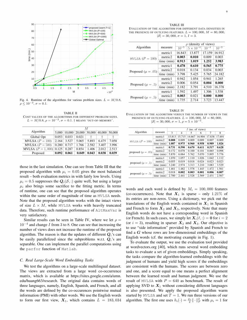
Fig. 4. Runtime of the algorithms for various problem sizes. L = M/0.8,ρ ≤ 10−3, σ = 0.1.

TABLE IICOST VALUES OF THE ALGORITHMS FOR DIFFERENT PROBLEM SIZES.L =M/0.8, ρ = 10−3 , σ = 0.1. † MEANS ‘OUT-OF-MEMORY’.

AlgorithmM

5,000 10,000 20,000 30,000 40,000 50,000Global Opt 0.053 0.033 0.021 † † †

MVLSA (P = 100) 2.164 3.527 5.065 5.893 6.475 7.058MVLSA (P = 500) 0.280 0.717 1.766 2.582 3.407 3.996

MVLSA (P = 1, 000) 0.125 0.287 0.854 1.406 2.012 2.513Proposed 0.092 0.061 0.049 0.043 0.038 0.039

those in the last simulation. One can see from Table III that theproposed algorithm with µi = 0.05 gives the most balancedresult – both evaluation metrics in with fairly low levels. Usingµi = 0.5 suppresses the Qi(S, :) quite well, but using a largerµi also brings some sacrifice to the fitting metric. In termsof runtime, one can see that the proposed algorithm operateswithin the same order of magnitude of time as MVLSA needs.Note that the proposed algorithm works with the intact viewsof size L ×M , while MVLSA works with heavily truncateddata. Therefore, such runtime performance of AltMaxVar isvery satisfactory.

Similar results can be seen in Table IV, where we let ρ =10−4 and change I from 3 to 8. One can see that increasing thenumber of views does not increase the runtime of the proposedalgorithm. The reason is that the updates of different Qi’s canbe easily parallelized since the subproblems w.r.t. Qi’s areseparable. One can implement the parallel computations usingthe parfor function of Matlab.

C. Real Large-Scale Word Embedding Tasks

We test the algorithms on a large-scale multilingual dataset.The views are extracted from a large word co-occurrencematrix, which is available at https://sites.google.com/a/umn.edu/huang663/research. The original data contains words ofthree languages, namely, English, Spanish, and French, and allthe words are defined by the co-occurences pointwise mutualinformation (PMI) with other words. We use the English wordsto form our first view, X1, which contains L = 183, 034

TABLE IIIEVALUATION OF THE ALGORITHM FOR DIFFERENT DATA DENSITIES INTHE PRESENCE OF OUTLYING FEATURES. L = 100, 000, M = 80, 000,

|S| = 30, 000, σ = 1, I = 3.

Algorithm measureρ (density of views)

10−5 5× 10−4 10−4 10−3

MVLSA (P = 100)

metric1 16.843 13.877 17.159 16.912metric2 0.003 0.010 0.009 0.003

time (min) 0.913 1.019 1.252 3.983

Proposed (µ = .05)

metric1 0.478 0.610 0.565 0.775metric2 0.018 0.134 0.034 0.003

time (min) 3.798 5.425 5.765 24.182

Proposed (µ = .1)

metric1 0.942 1.054 0.941 1.265metric2 0.006 0.054 0.004 0.000

time (min) 2.182 3.791 4.510 16.378

Proposed (µ = .5)

metric1 1.592 1.497 1.306 1.538metric2 0.003 0.021 0.000 0.000

time (min) 1.735 2.714 3.723 13.447

TABLE IVEVALUATION OF THE ALGORITHM VERSUS THE NUMBER OF VIEWS IN THE

PRESENCE OF OUTLYING FEATURES. L = 100, 000, M = 80, 000,|S| = 30, 000, σ = 1, ρ = 5× 10−5 .

Algorithm measureI (no. of views)

3 4 5 6 7 8

MVLSA (P = 100)

metric1 15.813 15.715 14.667 16.904 17.838 17.691metric2 0.008 0.009 0.009 0.009 0.007 0.009

time (min) 1.087 0.975 0.960 0.958 0.989 1.026

proposed (µ = .05)

metric1 0.731 0.590 0.670 0.611 0.517 0.628metric2 0.172 0.078 0.100 0.101 0.065 0.098

time (min) 5.870 6.064 5.762 5.070 5.895 5.776

proposed (µ = .1)

metric1 1.070 1.057 1.110 1.026 1.042 1.112metric2 0.055 0.019 0.018 0.024 0.023 0.023

time (min) 3.240 2.974 3.313 3.210 3.083 3.529

proposed (µ = .5)

metric1 1.461 1.482 1.578 1.443 1.472 1.561metric2 0.018 0.002 0.003 0.001 0.006 0.007

time (min) 2.700 2.441 2.528 2.569 2.431 2.567

words and each word is defined by Mi = 100, 000 features(co-occurrences). Note that X1 is sparse – only 1.21% ofits entries are non-zeros. Using a dictionary, we pick out thetranslations of the English words contained in X1 in Spanishand French to form X2 and X3, respectively. Note that manyEnglish words do not have a corresponding word in Spanish(or French). In such cases, we simply let Xi(`, :) = 0 for i = 2(or i = 3), resulting in sparser X2 and X3. Our objective isto use “side information” provided by Spanish and French tofind a G whose rows are low-dimensional embeddings of theEnglish words (cf. the motivating example in Fig. 1).

To evaluate the output, we use the evaluation tool providedat wordvectors.org [40], which runs several word embeddingtasks to evaluate a set of given embeddings. Simply speaking,the tasks compare the algorithm-learned embeddings with thejudgment of humans and yield high scores if the embeddingsare consistent with the humans. The scores are between zeroand one, and a score equal to one means a perfect alignmentbetween the learned result and human judgment. We use theresult of MVLSA with P = 640 as benchmark. The result ofapplying SVD to X1 without considering different languagesis also presented. We apply the proposed algorithm warmstarted by MVLSA and set T = 1. We run three versions of ouralgorithm. The first one uses hi(·) = µi

2 ‖ · ‖2F with µi = 1 for

10

i = 1, 2, 3. The second one uses hi(·) = µi‖ · ‖2,1 for i = 2, 3where µi = 0.05, and we have no regularization on the firstview. The third one is hi(·) = µi‖ · ‖1,1 for i = 2, 3 whereµi = 0.05. The reason for adding `2/`1 mixed-norm (and`1 norm) regularization to the French and Spanish views istwofold: First, the `2/`1 norm (`1 norm) promotes row sparsity(sparsity) of Qi and thus performs feature selection on X2

and X3 – this physically means that we aim at selecting themost useful features from the other languages to help enhanceEnglish word embeddings. Second, X2 and X3 are effectively“fat matrices” and thus a column-selective regularizer can helpimprove the conditioning. Interestingly, we find that not addingfeature-selective regularizations to the English view producesbetter results for the dataset considered. Our understanding isthat X1 is a complete view without missing elements, andthus giving Q1 more “degrees of freedom” helps improveperformance.

Tables V and VI show the word embedding results usingK = 50 and K = 100, respectively. One can see that using theinformation from multiple views does help in improving theword embeddings: For K = 50 and K = 100, the multiviewapproaches perform better relative to SVD in 11 and 12 tasksout of 12 tasks. In addition, the proposed algorithm with theregularizer hi(·) = µi/2‖ · ‖2F (denoted by `2) gives similaror slightly better performance on average in both experimentscompared to MVLSA. The proposed algorithm with the feature-selective regularizers (denoted by `2/`1 and `1, resp.) givesthe best evaluation results on both experiments – this suggeststhat for large-scale multilingual word embedding, feature se-lection is very meaningful. In particular, we observe that usinghi(Qi) = ‖Qi‖1,1 gives the best performance on many tasks.This further suggests that, in this case, different components ofthe reduced-dimension representations (i.e., columns of XiQi)may be better learned by using different features of the views.

VI. CONCLUSION AND FUTURE WORK

In this work, we revisited the MAX-VAR GCCA problemwith an eye towards scenarios involving large-scale and sparsedata. The proposed approach is memory-efficient and has lightper-iteration computational complexity if the views are sparse,and is thus suitable for dealing with big data. The algorithmis also flexible for incorporating different structure-promotingregularizers on the canonical components such as feature-selective regularizations. A thorough convergence analysis waspresented, showing that the proposed algorithmic frameworkguarantees a KKT point to be obtained at a sublinear con-vergence rate in general cases under a variety of structure-promoting regularizers. We also showed that the algorithmapproaches a global optimal solution at a linear convergencerate if the original MAX-VAR problem without regularizationis considered. Simulations and real experiments with large-scale multi-lingual data showed that the performance of theproposed algorithm is promising in dealing with real-worldlarge and sparse multiview data.

In the future, it is interesting to consider nonlinear operator-based multiview analysis, e.g., kernel (G)CCA [1] or deepneural network-based (G)CCA [41], under large-scale settings.

Nonlinear dimensionality reduction is very well-motivated inpractice since it is able to handle more complex modelsand usually performs well with real-life data. On the otherhand, the associated optimization problems are much harder,especially when the data dimension is large – which alsopromises a fertile research ground ahead. Another interestingdirection is to consider constraints on G (or XiQi) – insome applications, structured (e.g., sparse and nonnegative)low-dimensional representations of data are desired.

APPENDIX APROOF OF PROPOSITION 1

To simplify the notation, let us define Q = [QT1 , . . . ,Q

TI ]T

as a collection of Qi’s. We also rewrite the objective functionin (4) as

F (Q,G) = f(Q,G) + g(Q)

=

I∑i=1

fi(Qi,G) +

I∑i=1

gi(Qi),

where fi(Qi,G) and gi(Qi) are the smooth and non-smoothparts in (6) as before, and f(Q,G) =

∑Ii=1 fi(Qi,G) and

g(Q) =∑Ii=1 gi(Qi), respectively. Additionally, let

∇Q f(Q,G) = [(∇Q1f(Q,G))T , . . . , (∇QIf(Q,G))T ]T ,

∂Qg(Q) = [(∂Q1g1(Q1))T , . . . , (∂QI

gI(QI))T ]T .

As the algorithm is essentially a two-block alternating opti-mization (since Qi for all i are updated simultaneously), theabove notation suffices to describe the updates. Let

uQ

(Q; G, Q

)=f(G, Q) +

⟨∇Qf(Q, G),Q− Q

⟩+

I∑i=1

1

2αi‖Qi − Q‖2F +

I∑i=1

gi(Qi);

i.e., uQ(Q; G, Q

)is an approximation of F (G,Q) locally

at the point (G, Q). We further define uQ

(Q; G, Q

)=

uQ

(Q; G, Q

)−∑Ii=1 gi(Qi); i.e., uQ

(Q; G, Q

)is an ap-

proximation of the continuously differentiable part f(G,Q)locally at the point (G, Q). One can see that,

∇Qf(Q, G

)= ∇Qu

(Q; G, Q

), (14)

Since ∇Qifi(Qi,G) is Li-Lipschitz continuous w.r.t. Qi and

αi ≤ 1/Li for all i, we have the following holds:

uQ

(Q; G, Q

)≥ F

(Q, G

), ∀ Q, (15)

where the equality holds if and only if Qi = Qi for all i, i.e.,

uQ

(Q; G, Q

)= F

(Q, G

). (16)

Similarly, we define

uG

(G; G, Q

)=

I∑i=1

1

2

∥∥∥XiQ(r+1)i −G

∥∥∥2

F

+ ω ·∥∥∥G−G(r)

∥∥∥2

F+

I∑i=1

gi(Qi),

11

TABLE VEVALUATION ON 12 WORD EMBEDDING TASKS; K = 50.

TaskAlgorithm (K = 50)

SVD MVLSA AltMaxVar (`2) AltMaxVar (`2/`1) AltMaxVar (`1)EN-WS-353-SIM 0.63 0.69 0.67 0.68 0.69

EN-MC-30 0.56 0.63 0.63 0.64 0.66EN-MTurk-771 0.54 0.58 0.59 0.60 0.59

EN-MEN-TR-3k 0.67 0.66 0.67 0.68 0.69EN-RG-65 0.51 0.53 0.55 0.58 0.58

EN-MTurk-287 0.65 0.64 0.65 0.64 0.63EN-WS-353-REL 0.50 0.51 0.53 0.55 0.57

EN-VERB-143 0.21 0.22 0.21 0.21 0.20EN-YP-130 0.36 0.39 0.38 0.41 0.41

EN-SIMLEX-999 0.31 0.42 0.41 0.39 0.36EN-RW-STANFORD 0.39 0.43 0.43 0.43 0.43

EN-WS-353-ALL 0.56 0.59 0.59 0.60 0.62Average 0.49 0.52 0.53 0.54 0.54Median 0.53 0.56 0.57 0.59 0.59

TABLE VIEVALUATION ON 12 WORD EMBEDDING TASKS; K = 100.

TaskAlgorithm (K = 100)

SVD MVLSA AltMaxVar (`2) AltMaxVar (`2/`1) AltMaxVar (`1)EN-WS-353-SIM 0.68 0.72 0.71 0.72 0.72

EN-MC-30 0.73 0.68 0.72 0.74 0.82EN-MTurk-771 0.59 0.60 0.60 0.61 0.62

EN-MEN-TR-3k 0.72 0.70 0.70 0.71 0.73EN-RG-65 0.68 0.63 0.64 0.68 0.70

EN-MTurk-287 0.61 0.66 0.65 0.64 0.64EN-WS-353-REL 0.57 0.54 0.55 0.56 0.59

EN-VERB-143 0.19 0.28 0.27 0.29 0.28EN-YP-130 0.42 0.41 0.41 0.45 0.49

EN-SIMLEX-999 0.34 0.42 0.41 0.41 0.39EN-RW-STANFORD 0.44 0.46 0.45 0.46 0.48

EN-WS-353-ALL 0.62 0.62 0.62 0.62 0.65Average 0.55 0.56 0.56 0.58 0.59Median 0.60 0.61 0.61 0.62 0.63

where we recall that ω = (1−γ)I/2γ and the last term is aconstant if Q is fixed.

The update rule of G in Algorithm 1 can be re-expressedas G ∈ arg minGTG=I uG

(G; G, Q

). It is easily seen that

uG

(G; G, Q

)≥ F

(Q,G

), (17a)

uG

(G; G, Q

)= F

(Q, G

). (17b)

Hence, Algorithm 1 boils down to

Q(r,t+1)i = arg min

Qi

uQ

(Q;G(r),Q(r,t)

), ∀t (18a)

G(r+1) ∈ arg minGTG=I

uG

(G;G(r),Q(r+1)

). (18b)

When γ = 1, (18b) amounts to SVD of∑Ii=1 XiQi/I

and the G-subproblem minGTG=I F (Q(r+1),G) is optimallysolved; otherwise, both (18a) and (18b) are local upper boundminimizations.

Note that the following holds:

F(Q(r),G(r)

)= uQ(Q(r);G(r),Q(r)) (19a)

≥ uQ(Q(r+1);G(r),Q(r,T−1)) (19b)

≥ F(Q(r+1),G(r)

)(19c)

= uG

(G(r);G(r),Q(r+1)

)(19d)

≥ uG(G(r+1);G(r),Q(r+1)

)(19e)

≥ F(Q(r+1),G(r+1)

), (19f)

where (19a) holds because of (16), (19b) holds since PG isa descending method when αi ≤ 1/Li [42], (19c) holds bythe property in (16), (19d) holds due to (17), (19e) is due tothe fact that (18b) is optimally solved, and (19f) holds alsobecause of the first equation in (17).

Next, we show that every limit point is a KKT point.Assume that there exists a convergent subsequence of{G(r),Q(r)}r=0,1,..., whose limit point is (G∗,Q∗) and thesubsequence is indexed by {rj}j=1,...,∞. We have the follow-

12

ing chain of inequalities:

uQ

(Q;G(rj),Q(rj)

)≥ uQ

(Q(rj ,1);G(rj),Q(rj)

)(20a)

≥ uQ(Q(rj ,T );G(rj),Q(rj ,T−1)

)(20b)

≥ F (G(rj),Q(rj+1)) (20c)

≥ F(Q(rj+1),G(rj+1)

)(20d)

≥ F(Q(rj+1),G(rj+1)

)(20e)

= uQ

(Q(rj+1);G(rj+1),Q(rj+1)

),

(20f)

where (20a) holds because of the update rule in (18a), (20b)holds, again, by the descending property of PG, (20d) follows(19f), and (20f) is again because of the way that we constructuQ(Q;G(rj+1) ,Q(rj+1)). Taking j → ∞, and by continuityof uQ(·), we have

uQ(Q;G∗,Q∗) ≥ uQ(Q∗;G∗,Q∗), (21)

i.e., Q∗ is a minimum of uQ(Q;G∗,Q∗). Consequently,Q∗ satisfies the conditional KKT conditions, i.e., 0 ∈∇QuQ(Q∗;G∗,Q∗) + ∂Qg(Q∗), which, by (14), also means

0 ∈ ∇Qifi(Q

∗i ,G

∗) + ∂Qigi(Q

∗i ), ∀i. (22)

We now show that Q(rj ,t) for t = 1, . . . , T also convergesto Q∗. Indeed, we have

uQ(Q(rj+1);G(rj+1),Q(rj+1)) ≤ uQ(Q(rj ,1);G(rj),Q(rj))

≤ uQ(Q(rj);G(rj),Q(rj)),

where the first inequality was derived from (20). Taking j →∞, we see that uQ(Q∗;G∗,Q∗) ≤ uQ(Q(rj ,1);G∗,Q∗) ≤uQ(Q∗;G∗,Q∗), which implies that uQ(Q(rj ,1);G∗,Q∗) =uQ(Q∗;G∗,Q∗) ≤ uQ(Q;G∗,Q∗). On the other hand, theproblem in (18a) has a unique minimizer when gi(·) is aconvex closed function [34], which means that Q(rj ,1) →Q∗. By the same argument, we can show that Q(rj ,t) fort = 1, . . . , T also converges to Q∗. Consequently, we haveQ(rj ,T ) = Q(rj+1) → Q∗. We repeat the proof in (20) to G:

uG

(G;G(rj),Q(rj+1)

)≥ uG

(G(rj+1);G(rj),Q(rj+1)

)≥ F (Q(rj+1),G(rj+1))

≥ F(Q(rj+1),G(rj+1)

)= uG

(G(rj+1);G(rj+1),Q(rj+1)

),

Taking j →∞ and by Q(rj+1) → Q∗, we have

uG (G;G∗,Q∗) ≥ uG (G∗;G∗,Q∗) , ∀GTG = I.

The above means that G∗ satisfies the partial conditionalKKT conditions w.r.t. G. Combining with (22), we see that(G∗,Q∗) is a KKT point of the original problem.

Now, we show the b) part. First, we show that Qi remainsin a bounded set (the variable G is always bounded since wekeep it feasible in each iteration). Since the objective valueis non-increasing (cf. Proposition 1), if we denote the initial

objective value as V , then F (G(r),Q(r)) ≤ V holds in all sub-sequent iterations. Note that when X

(0)i and Q

(0)i are bounded,

V is also finite. In particular, we have ‖XiQi −G‖2F +

2∑Ii=1 gi(Qi) ≤ 2V holds, which implies ‖XiQi‖F ≤

‖G‖F +√

2V by the triangle inequality. The right-hand sideis finite since both terms are bounded. Denote (‖G‖F +

√2V )

by V ′. Then, we have ‖Qi‖F = ‖(XTi Xi)

−1XTi XiQi‖F ≤

‖(XTi Xi)

−1XTi ‖F · ‖XiQi‖F ≤ V ′ · ‖(XT

i Xi)−1XT

i ‖F .Now, by the assumption that rank(Xi) = Mi, the term‖(XT

i Xi)−1XT

i ‖F is bounded. This shows that ‖Qi‖F isbounded. Hence, starting from a bounded Q

(0)i , the solution

sequence {Q(r),G(r)} remains in a bounded set. Since theconstraints of Qi, i.e., RMi×K and G are also closed sets,{Q(r),G(r)} remains in a compact set.

Now, let us denote K as the set containing all the KKTpoints. Suppose the whole sequence does not converge toK. Then, there exists a convergent subsequence indexed by{rj} such that limj→∞ d(r)(K) ≥ γ for some positive γ,where d(r)(K) = minY ∈K ‖(G(r),Q(r)) − Y ‖. Since thesubsequence indexed by {rj} lies in a closed and boundedset as we have shown, this subsequence has a limit point.However, as we have shown in Theorem 1, every limit point ofthe solution sequence is a KKT point. This is a contradiction.Therefore, the whole sequence converges to a KKT point.

APPENDIX BPROOF OF LEMMA 1

First, we have the update rule Q(r,t+1)i = Q

(r,t)i −

αi∇QiF (Q

(r,t)i ,G(r)), which leads to the following:

1

αi(Q

(r,t+1)i −Q

(r,t)i ) = −∇QiF (Q

(r,t)i ,G(r)). (24)

Meanwhile, the updating rule can also be expressed as

Q(r,t+1)i = arg min

Qi

⟨∇Qif(Q

(r,t)i ,G(r)),Qi −Q

(r,t)i

⟩+ gi(Qi) +

1

2αi‖Qi −Q

(r,t)i ‖2F . (25)

Therefore, there exists a ∂Qigi(Q

(r,t+1)) and a Q(r,t+1)

satisfy the following optimality conditions:

0 = ∇Qifi(Q

(r,t)i ,G(r)) + ∂Qi

gi(Q(r,t+1)i ) +

1

αi(Q

(r,t+1)i −Q

(r,t)i ).

Consequently, we see that

I∑i=1

T∑t=0

∥∥∥∇QiF (Q

(r,t)i ,G(r))

∥∥∥2

F→ 0

⇒ Q(r,t)i −Q

(r,t+1)i → 0, ∀ t = 0, . . . , T − 1

⇒ Q(r)i −Q

(r+1)i → 0, ∀i

⇒ ∇Q f(Q(r),G(r)

)+ ∂Qg

(Q(r)

)→ 0

which holds since T is finite. The above means that 0 ∈∇Qf(Q(r),G(r))+∂Qg(Q(r)) is satisfied when Z(r+1) → 0.

13

Recall that G(r+1) satisfies the optimality condition ofProblem (10). Therefore, there exists a Λ(r+1) such that thefollowing optimality condition holds

G(r) −I∑i=1

XiQ(r+1)i /I +

1

γ

(G(r+1) −G(r)

)+ G(r+1)Λ(r+1) = 0 (26)

Combining (26) and (24), we have

Z(r+1) =1

γ2

∥∥∥G(r+1) −G(r)∥∥∥2

F+

I∑i=1

1

α2i

∥∥∥Q(r+1)i −Q

(r)i

∥∥∥2

F.

We see that Z(r+1) → 0 implies that a KKT point is reachedand this completes the proof of Lemma 1.

APPENDIX CPROOF OF THEOREM 1

We show that every iterate of Q and G gives sufficient de-creases of the overall objective function. Since ∇Qifi(Qi,G)is Li-Lipschitz continuous for all i, we have the following:

F (Q(r,t+1),G(r)) ≤ uQ(Q(r,t+1);G(r),Q(r,t)

). (27)

= f(Q(r,t),G(r)) +⟨∇Qf(Q(r,t),G(r)),Q(r,t+1) −Q(r)

⟩+

I∑i=1

gi

(Q

(r,t+1)i

)+

I∑i=1

Li2

∥∥∥Q(r,t+1)i −Q

(r,t)i

∥∥∥2

F.

Since Q(r,t+1) is a minimizer of Problem (25), we also have⟨∇Qf(Q(r,t),G(r)),Q(r,t+1) −Q(r,t)

⟩+

I∑i=1

gi(Q(r,t+1)i )

+

I∑i=1

1

2αi

∥∥∥Q(r,t+1)i −Q

(r,t)i

∥∥∥2

F≤

I∑i=1

gi(Q(r,t)i ), (28)

which is obtained by letting Qi = Q(r,t)i . Combining (27) and

(28), we have

F (Q(r,t+1),G(r))− F (Q(r,t),G(r))

≤ −I∑i=1

(1

2αi− Li

2

)∥∥∥Q(r,t+1)i −Q

(r,t)i

∥∥∥2

F.

(29)

Summing up the above over t = 0, . . . , T − 1, we have

F (Q(r),G(r))− F (Q(r+1),G(r))

≥T−1∑t=0

I∑i=1

(1

2αi− Li

2

)∥∥∥Q(r,t+1)i −Q

(r,t)i

∥∥∥2

F.

(30)

For the G-subproblem, we have

uG(G(r+1);G(r),Q(r+1)) ≤ uG(G(r);G(r),Q(r+1))

= F (G(r),Q(r+1))

and thus

F (G(r+1),Q(r+1)) +ω‖G(r+1)−Gr‖2F ≤ F (Q(r+1),G(r)),

or, equivalently

F (Q(r+1),G(r+1))− F (Q(r+1),G(r))

≤ −ω∥∥∥G(r+1) −G(r)

∥∥∥2

F, ∀GTG = I,

(31)

where ω =(I

2γ −I2

)> 0 if γ < 1. Combining (30) and (31),

we have

F (Q(r),G(r))− F (Q(r+1),G(r+1))

≥(I

2γ− I

2

)∥∥∥G(r+1) −G(r)∥∥∥2

F

+

T−1∑t=0

I∑i=1

(1

2αi− Li

2

)∥∥∥Q(r,t+1)i −Q

(r,t)i

∥∥∥2

F.

(32)

Summing up F (Q(r),G(r)) over r = 0, 1, . . . , J − 1, wehave the following:

F (Q(r),G(r))− F (Q(r+1),G(r+1))

≥J−1∑r=0

ω∥∥∥G(r+1) −G(r)

∥∥∥2

F

+

J−1∑r=0

T−1∑t=0

I∑i=1

(1

2αi− Li

2

)∥∥∥Q(r,t+1)i −Q

(r,t)i

∥∥∥2

F.

=

J−1∑r=0

ωγ2

∥∥∥∥∥G(r) −∑Ii=1 XiQ

(r+1)i

I+ G(r+1)Λ(r+1)

∥∥∥∥∥2

F

+

J−1∑r=0

I∑i=1

T−1∑t=0

(1

2αi− Li

2

)α2i

∥∥∥∇QiF (Q(r,t),G(r))

∥∥∥2

F

≥J−1∑r=0

cZ(r+1), (33)

where c = min{ωγ2, {( 12αi− Li

2 )α2i }i=1,...,I}. By the defini-

tion of J , we have

F (Q(0),G(0))− F (Q(J),G(J))

J − 1≥∑J−1r=0 cZ

(r+1)

J − 1≥ c · δ

⇒ δ ≤ 1

c

F (Q(0),G(0))− FJ − 1

⇒ δ ≤ v

J − 1,

where F is the lower bound of the cost function and v =(F (Q(0),G(0))−F )/c. This completes the proof.

APPENDIX DPROOF OF THEOREM 2

First consider an easier case where ε(r) = 0 for all r. Then,we have Q

(r+1)i = (XT

i Xi+µiI)−1XTi G

(r). Therefore, theupdate w.r.t. G is simply to apply SVD on

∑Ii=1 XiQi/I =

MG(r)/I . In other words, there exists an invertible Θ(r+1)

such thatG(r+1)Θ(r+1) = MG(r), (34)

where M =∑Ii=1 XiX

†i as before, since the SVD proce-

dure is nothing but a change of bases. The update rule in(34), is essentially the orthogonal iteration algorithm in [30].Invoking [30, Theorem 8.2.2], one can show that ‖UT

2 G(r)‖2approaches zero linearly.

14

The proof of the case where ε(r) > 0 can be consideredas an extension of round-off error analysis of orthogonaliterations, and can be shown following the insights of [17]and [43] with proper modifications to accommodate the MAX-VAR GCCA case. At the rth iteration, ideally, we haveQ

(r+1)i = (XT

i Xi + µiI)−1XTi G

(r) if the Q-subproblem issolved to optimality. In practice, what we have is an inexactsolution, i.e.,

Q(r+1)i = (XT

i Xi + µiI)−1XTi G

(r) + W(r)i ,

where we have assumed that the largest singular value of W (r)i

is bounded by ε, i.e., ‖W (r)i ‖2 ≤ ε. Hence, one can see that

I∑i=1

XiQ(r+1)i = MG(r) +

I∑i=1

XiW(r)i .

Therefore, following the same reason of obtaining (34), wehave

G(r+1)Θ(r+1) =

(MG(r) +

I∑i=1

XiW(r)i

),

where Θ(r+1) ∈ RK×K is a full-rank matrix since the solutionvia SVD is a change of bases. Consequently, we have[UT

1 G(r+1)

UT2 G(r+1)

]Θ(r+1) =

[Λ1U

T1 G(r) + UT

1

∑Ii=1 XiW

(r)i

Λ2UT2 G(r) + UT

2

∑Ii=1 XiW

(r)i

].

Now, we denote

∆(r)1 = UT

1

I∑i=1

XiW(r)i , ∆

(r)2 = UT

2

I∑i=1

XiW(r)i ,

as two error terms at the rth iteration. Next, let us considerthe following chain of inequalities:∥∥∥∥UT

2 G(r+1)(UT

1 G(r+1))−1

∥∥∥∥2

(35)

=

∥∥∥∥(Λ2UT2 G(r) + ∆

(r)2

)(Λ1U

T1 G(r) + ∆

(r)1

)−1∥∥∥∥

2

≤

∥∥∥(Λ2UT2 G(r) + ∆

(r)2

)(UT

1 G(r))−1∥∥∥

2

σK

(Λ1 + ∆

(r)1 (UT

1 G(r))−1)

≤λK+1

∥∥∥UT2 G(r)

(UT

1 G(r))−1∥∥∥

2+ ‖∆(r)

2

(UT

1 G(r))−1 ‖2

λK − ‖∆(r)1

(UT

1 G(r))−1 ‖2

≤∥∥∥∥UT

2 G(r)(UT

1 G(r))−1

∥∥∥∥2

λK+1 +‖∆(r)

2 ‖2σmin(UT

2 G(r))

λK − ‖∆(r)1 ‖2

σmax(UT1 G(r))

.

(36)

Assume that the following holds:

max{‖∆(r)1 ‖2, ‖∆

(r)2 ‖2} (37)

≤ λK − λK+1

3min

{σmin

(UT

2 G(r)), σmax

(UT

1 G(r))}

.

Then, one can easily show that∥∥∥∥UT2 G(r+1)

(UT

1 G(r+1))−1

∥∥∥∥2

≤ %∥∥∥∥UT

2 G(r)(UT

1 G(r))−1

∥∥∥∥2

(38)

where

% =

(2λK+1 + λK2λK + λK+1

)< 1.

One can see that∥∥∥UT2 G(r+1)

∥∥∥2≤∥∥∥∥UT

2 G(r+1)(UT

1 G(r+1))−1

∥∥∥∥2

≤ %r∥∥∥∥(UT

2 G(0))(UT

1 G(0))−1

∥∥∥∥2

≤ %r tan(θ), (39)

where the first inequality holds because of ‖UT1 G(r+1)‖2 ≤ 1.

By noticing that ‖UT2 G(0)‖2 = sin(θ) and ‖(UT

1 G(0))−1‖2 =1/ cos(θ) [30, Theorem 8.2.2], we obtain the last inequality.

In addition, we notice that

max{‖∆(r)1 ‖2, ‖∆

(r)2 ‖2} ≤

I∑i=1

λmax(Xi)ε(r).

This means that to ensure linear convergence to a globalminimal solution, it suffices to have

ε(r) ≤ λK − λK+1

3∑Ii=1 λmax(Xi)

(40)

×min{σmin

(UT

2 G(r)), σmax

(UT

1 G(r))}

in the worst case.The last piece of the proof is to show that (UT

1 G(r))−1

in (36) always exists. Note that if (39) holds, then UT1 G(r)

is always invertible under the condition stated in (12). Thereason is that we always have [30]

σ2max(UT

2 G(r)) + σ2min(UT

1 G(r)) = 1.

Therefore, σ2min(UT

1 G(r)) monotonically increases sinceσmax(UT

2 G(r)) decreases when (40) (and thus (39)) holds.Hence, if σmin(UT

1 G(0)) > 0, we have σmin(UT1 G(r)) > 0

for all r > 1.

REFERENCES

[1] D. R. Hardoon, S. Szedmak, and J. Shawe-Taylor, “Canonical correlationanalysis: An overview with application to learning methods,” Neuralcomputation, vol. 16, no. 12, pp. 2639–2664, 2004.

[2] Y.-O. Li, T. Adali, W. Wang, and V. D. Calhoun, “Joint blind sourceseparation by multiset canonical correlation analysis,” IEEE Trans.Signal Process., vol. 57, no. 10, pp. 3918–3929, 2009.

[3] A. Bertrand and M. Moonen, “Distributed canonical correlation analysisin wireless sensor networks with application to distributed blind sourceseparation,” IEEE Trans. Signal Process., vol. 63, no. 18, pp. 4800–4813,2015.

[4] Q. Wu and K. M. Wong, “Un-music and un-cle: An application ofgeneralized correlation analysis to the estimation of the direction ofarrival of signals in unknown correlated noise,” IEEE Trans. SignalProcess., vol. 42, no. 9, pp. 2331–2343, 1994.

[5] A. Dogandzic and A. Nehorai, “Finite-length mimo equalization usingcanonical correlation analysis,” IEEE Trans. Signal Process., vol. 50,no. 4, pp. 984–989, 2002.

15

[6] S. M. Kakade and D. P. Foster, “Multi-view regression via canonicalcorrelation analysis,” in Learning Theory. Springer, 2007, pp. 82–96.

[7] K. Chaudhuri, S. M. Kakade, K. Livescu, and K. Sridharan, “Multi-viewclustering via canonical correlation analysis,” in Proc. ICML. ACM,2009, pp. 129–136.

[8] R. Arora and K. Livescu, “Multi-view learning with supervision fortransformed bottleneck features,” in Proc. ICASSP. IEEE, 2014, pp.2499–2503.

[9] H. Wang, T. Lee, C.-C. Leung, B. Ma, and H. Li, “Acoustic segmentmodeling with spectral clustering methods,” IEEE/ACM Trans. Audio,Speech, Language Process., vol. 23, no. 2, pp. 264–277, 2015.

[10] P. Rastogi, B. Van Durme, and R. Arora, “Multiview LSA: Representa-tion learning via generalized CCA,” in Proc. NAACL, 2015.

[11] J. D. Carroll, “Generalization of canonical correlation analysis to threeor more sets of variables,” in Proc. annual convention of the AmericanPsychological Association, vol. 3, 1968, pp. 227–228.

[12] P. Horst, “Generalized canonical correlations and their applications toexperimental data,” Journal of Clinical Psychology, vol. 17, no. 4, pp.331–347, 1961.

[13] J. R. Kettenring, “Canonical analysis of several sets of variables,”Biometrika, vol. 58, no. 3, pp. 433–451, 1971.

[14] N. A. Asendorf, “Informative data fusion: Beyond canonical correlationanalysis,” Ph.D. dissertation, The University of Michigan, 2015.

[15] Z. Ma, Y. Lu, and D. Foster, “Finding linear structure in largedatasets with scalable canonical correlation analysis,” arXiv preprintarXiv:1506.08170, 2015.

[16] L. Sun, S. Ji, and J. Ye, “Canonical correlation analysis for multilabelclassification: A least-squares formulation, extensions, and analysis,”IEEE Trans. Pattern Anal. Machine Intel., vol. 33, no. 1, pp. 194–200,2011.

[17] Y. Lu and D. P. Foster, “Large scale canonical correlation analysis withiterative least squares,” in Proc. NIPS, 2014, pp. 91–99.

[18] M. Van De Velden and T. H. A. Bijmolt, “Generalized canonicalcorrelation analysis of matrices with missing rows: a simulation study,”Psychometrika, vol. 71, no. 2, pp. 323–331, 2006.

[19] D. R. Hardoon and J. Shawe-Taylor, “Sparse canonical correlationanalysis,” Machine Learning, vol. 83, no. 3, pp. 331–353, 2011.

[20] D. M. Witten, R. Tibshirani, and T. Hastie, “A penalized matrixdecomposition, with applications to sparse principal components andcanonical correlation analysis,” Biostatistics, p. kxp008, 2009.

[21] X. Chen, H. Liu, and J. G. Carbonell, “Structured sparse canonical cor-relation analysis,” in International Conference on Artificial Intelligenceand Statistics, 2012, pp. 199–207.

[22] D. M. Witten and R. J. Tibshirani, “Extensions of sparse canonicalcorrelation analysis with applications to genomic data,” Statistical ap-plications in genetics and molecular biology, vol. 8, no. 1, pp. 1–27,2009.

[23] M. Faruqui and C. Dyer, “Improving vector space word representationsusing multilingual correlation.” Association for Computational Lin-guistics, 2014.

[24] C. Sigg, B. Fischer, B. Ommer, V. Roth, and J. Buhmann, “Nonnegativecca for audiovisual source separation,” in 2007 IEEE Workshop onMachine Learning for Signal Processing. IEEE, 2007, pp. 253–258.

[25] B. Fischer, V. Roth, and J. M. Buhmann, “Time-series alignment bynon-negative multiple generalized canonical correlation analysis,” BMCbioinformatics, vol. 8, no. Suppl 10, p. S4, 2007.

[26] X. Fu, K. Huang, M. Hong, N. D. Sidiropoulos, and A. M.-C. So,“Scalable and flexible max-var generalized canonical correlation analysisvia alternating optimization,” in Proc. ICASSP 2017, 2016.

[27] J. Rupnik, P. Skraba, J. Shawe-Taylor, and S. Guettes, “A comparison ofrelaxations of multiset cannonical correlation analysis and applications,”arXiv preprint arXiv:1302.0974, 2013.

[28] L.-H. Zhang, L.-Z. Liao, and L.-M. Sun, “Towards the global solutionof the maximal correlation problem,” Journal of Global Optimization,vol. 49, no. 1, pp. 91–107, 2011.

[29] X. Fu, K. Huang, E. E. Papalexakis, H. A. Song, P. P. Talukdar, N. D.Sidiropoulos, C. Faloutsos, and T. Mitchell, “Efficient and distributedalgorithms for large-scale generalized canonical correlations analysis,”in Proc. IEEE ICDM 2016, Dec 2016, pp. 871–876.

[30] G. H. Golub and C. F. V. Loan., Matrix Computations. The JohnsHopkins University Press, 1996.

[31] I. Rustandi, M. A. Just, and T. Mitchell, “Integrating multiple-studymultiple-subject fmri datasets using canonical correlation analysis,” inProceedings of the MICCAI 2009 Workshop: Statistical modeling anddetection issues in intra-and inter-subject functional MRI data analysis,2009.

[32] T. M. Mitchell, S. V. Shinkareva, A. Carlson, K.-M. Chang, V. L.Malave, R. A. Mason, and M. A. Just, “Predicting human brain activityassociated with the meanings of nouns,” science, vol. 320, no. 5880, pp.1191–1195, 2008.

[33] S. Boyd, N. Parikh, E. Chu, B. Peleato, and J. Eckstein, “Distributedoptimization and statistical learning via the alternating direction methodof multipliers,” Foundations and Trends in Machine Learning, pp. 1–122, 2011.

[34] N. Parikh and S. Boyd, “Proximal algorithms,” Foundations and Trendsin optimization, vol. 1, no. 3, pp. 123–231, 2013.

[35] P. Schonemann, “A generalized solution of the orthogonal Procrustesproblem,” Psychometrika, vol. 31, no. 1, pp. 1–10, 1966.

[36] D. P. Bertsekas, Nonlinear programming. Athena Scientific, 1999.[37] M. Razaviyayn, M. Hong, and Z.-Q. Luo, “A unified convergence

analysis of block successive minimization methods for nonsmoothoptimization,” SIAM Journal on Optimization, vol. 23, no. 2, pp. 1126–1153, 2013.

[38] Y. Xu and W. Yin, “A block coordinate descent method for regularizedmulticonvex optimization with applications to nonnegative tensor fac-torization and completion,” SIAM Journal on imaging sciences, vol. 6,no. 3, pp. 1758–1789, 2013.

[39] ——, “A globally convergent algorithm for nonconvex optimizationbased on block coordinate update,” arXiv preprint arXiv:1410.1386,2014.

[40] M. Faruqui and C. Dyer, “Community evaluation and exchange ofword vectors at wordvectors.org,” in Proc. 52nd Annual Meeting ofthe Association for Computational Linguistics: System Demonstrations.Baltimore, USA: Association for Computational Linguistics, June 2014.

[41] G. Andrew, R. Arora, J. A. Bilmes, and K. Livescu, “Deep canonicalcorrelation analysis.” in ICML (3), 2013, pp. 1247–1255.

[42] A. Beck and M. Teboulle, “A fast iterative shrinkage-thresholding algo-rithm for linear inverse problems,” SIAM journal on imaging sciences,vol. 2, no. 1, pp. 183–202, 2009.

[43] R. Ge, C. Jin, S. M. Kakade, P. Netrapalli, and A. Sidford, “Efficientalgorithms for large-scale generalized eigenvector computation andcanonical correlation analysis,” in ICML 2016, 2016.

Xiao Fu (S’12-M’15) received his B.Eng and M.Engdegrees in Communications and Information Engi-neering from the University of Electronic Scienceand Technology of China, Chengdu, China, in 2005and 2010, respectively. In 2014, he received hisPh.D. degree in Electronic Engineering from TheChinese University of Hong Kong (CUHK), Shatin,N.T., Hong Kong. From 2005 to 2006, he wasan Assistant Engineer at China Telecom Co. Ltd.,Shenzhen, China. He is currently a Postdoctoral As-sociate at the Department of Electrical and Computer

Engineering, University of Minnesota, Minneapolis, MN 55455, United States.His research interests include signal processing and machine learning, with arecent emphasis on factor analysis and its applications.

Dr. Fu received a Best Student Paper Award at IEEE ICASSP 2014, andwas a finalist of the Best Student Paper Competition at IEEE SAM 2014. Healso co-authored a paper that received a Best Student Paper Award at IEEECAMSAP 2015.

Kejun Huang (S’13-M’17) received the bachelor’sdegree from Nanjing University of Information Sci-ence and Technology, Nanjing, China in 2010. Hereceived the Ph.D. degree in Electrical Engineeringfrom University of Minnesota, Minneapolis, MN,USA in 2016. He is currently a Postdoctoral Asso-ciate at the Department of Electrical and ComputerEngineering, University of Minnesota, Minneapolis,United States. His research interests include signalprocessing, machine learning, and optimization.

16

Mingyi Hong received his B.E. degree in Com-munications Engineering from Zhejiang University,China, in 2005, his M.S. degree in Electrical En-gineering from Stony Brook University in 2007,and Ph.D. degree in Systems Engineering fromUniversity of Virginia in 2011. From 2011 to 2014he has been a Post Doctoral Fellow and a Re-search Assistant Professor with the Department ofElectrical and Computer Engineering, University ofMinnesota, Twin Cities. He is currently an AssistantProfessor with the Department of Industrial and

Manufacturing Systems Engineering (IMSE), Iowa State University, Ames.His research interests include signal processing, wireless communications,large-scale optimization and its applications in compressive sensing, complexnetworks and high-dimensional data analysis.

Nicholas D. Sidiropoulos (F’09) received theDiploma in Electrical Engineering from the Aris-totelian University of Thessaloniki, Greece, andM.S. and Ph.D. degrees in Electrical Engineeringfrom the University of Maryland - College Park,in 1988, 1990 and 1992, respectively. He servedas Assistant Professor at the University of Virginia(1997-1999); Associate Professor at the Universityof Minnesota - Minneapolis (2000-2002); Professorat the Technical University of Crete, Greece (2002-2011); and Professor at the University of Minnesota

- Minneapolis (2011-). His current research focuses primarily on signal andtensor analytics, with applications in cognitive radio, big data, and preferencemeasurement. He received the NSF/CAREER award (1998), the IEEE SignalProcessing Society (SPS) Best Paper Award (2001, 2007, 2011), and theIEEE SPS Meritorious Service Award (2010). He has served as IEEE SPSDistinguished Lecturer (2008-2009), and Chair of the IEEE Signal Processingfor Communications and Networking Technical Committee (2007-2008). Hereceived the Distinguished Alumni Award of the Department of Electrical andComputer Engineering, University of Maryland, College Park in 2013, andwas elected EURASIP Fellow in 2014.

Anthony Man-Cho So (M’12–SM’17) received hisBSE degree in Computer Science from PrincetonUniversity with minors in Applied and Computa-tional Mathematics, Engineering and ManagementSystems, and German Language and Culture. Hethen received his MSc degree in Computer Scienceand his PhD degree in Computer Science with a PhDminor in Mathematics from Stanford University. Dr.So joined The Chinese University of Hong Kong(CUHK) in 2007. He is currently an Assistant Deanof the Faculty of Engineering and an Associate

Professor in the Department of Systems Engineering and Engineering Man-agement. He also holds a courtesy appointment as an Associate Professorin the CUHK-BGI Innovation Institute of Trans-omics. His research focuseson the interplay between optimization theory and various areas of algorithmdesign, such as computational geometry, machine learning, signal processing,bioinformatics, and algorithmic game theory.

Dr. So currently serves on the editorial boards of Journal of GlobalOptimization, Optimization Methods and Software, and SIAM Journal onOptimization. He has also served on the editorial boards of IEEE TRANS-ACTIONS ON SIGNAL PROCESSING and Mathematics of Operations Research.He received the 2015 IEEE Signal Processing Society Signal Processing Mag-azine Best Paper Award, the 2014 IEEE Communications Society Asia-PacificOutstanding Paper Award, the 2010 Institute for Operations Research and theManagement Sciences (INFORMS) Optimization Society Optimization Prizefor Young Researchers, and the 2010 CUHK Young Researcher Award. Healso received the 2008 Exemplary Teaching Award and the 2011, 2013, 2015Dean’s Exemplary Teaching Award from the Faculty of Engineering at CUHK,and the 2013 Vice-Chancellor’s Exemplary Teaching Award from CUHK.