
SC07 CUDA 3 Libraries - GPGPU · releases CPU-side resources used by the CUBLAS library. The...
35
1 S05: High Performance Computing with CUDA CUDA Libraries CUDA Libraries Massimiliano Fatica, NVIDIA 2 S05: High Performance Computing with CUDA Outline Outline CUDA libraries: CUBLAS: BLAS implementation CUFFT: FFT implementation Using CUFFT to solve a Poisson equation with spectral methods: How to use the profile Optimization steps Accelerating MATLAB code with CUDA
Transcript of SC07 CUDA 3 Libraries - GPGPU · releases CPU-side resources used by the CUBLAS library. The...
1
S05: High Performance Computing with CUDA
CUDA LibrariesCUDA Libraries
Massimiliano Fatica, NVIDIA
2S05: High Performance Computing with CUDA
OutlineOutline
CUDA libraries:CUBLAS: BLAS implementationCUFFT: FFT implementation
Using CUFFT to solve a Poisson equation with spectral methods:
How to use the profileOptimization steps
Accelerating MATLAB code with CUDA
2
3S05: High Performance Computing with CUDA
CUBLASCUBLASCUBLAS is an implementation of BLAS (Basic Linear Algebra Subprograms) on top of the CUDA driver. It allows access to the computational resources of NVIDIA GPUs.
The library is self-contained at the API level, that is, no direct interaction with the CUDA driver is necessary.
The basic model by which applications use the CUBLAS library is to:•create matrix and vector objects in GPU memory space,•fill them with data, •call a sequence of CUBLAS functions, •upload the results from GPU memory space back to the host.
CUBLAS provides helper functions for creating and destroying objects in GPU space, and for writing data to and retrieving data from these objects.
4S05: High Performance Computing with CUDA
Supported featuresSupported features
• BLAS functions implemented (single precision only): •Real data: level 1, 2 and 3•Complex data: level1 and CGEMM
(Level 1=vector vector O(N), Level 2= matrix vector O(N2), Level 3=matrix matrix O(N3) )
• For maximum compatibility with existing Fortran environments, CUBLAS uses column-major storage, and 1-based indexing:
Since C and C++ use row-major storage, this means applications cannot use the native C array semantics for two-dimensional arrays. Instead, macros or inline functions should be defined to implement matrices on top of one-dimensional arrays.
3
5S05: High Performance Computing with CUDA
Using CUBLASUsing CUBLAS
•The interface to the CUBLAS library is the header file cublas.h
•Function names: cublas(Original name).cublasSgemm
•Because the CUBLAS core functions (as opposed to the helper functions) do not return error status directly, CUBLAS provides a separate function to retrieve the last error that was recorded, to aid in debugging
•CUBLAS is implemented using the C-based CUDA tool chain, and thus provides a C-style API. This makes interfacing to applications written in C or C++ trivial.
6S05: High Performance Computing with CUDA
cublasInitcublasInit, , cublasShutdowncublasShutdowncublasStatus cublasInit()
initializes the CUBLAS library and must be called before any other CUBLAS API function is invoked. It allocates hardware resources necessary for accessing the GPU.
cublasStatus cublasShutdown()
releases CPU-side resources used by the CUBLAS library. The release of GPU-side resources may be deferred until the application shuts down.
4
7S05: High Performance Computing with CUDA
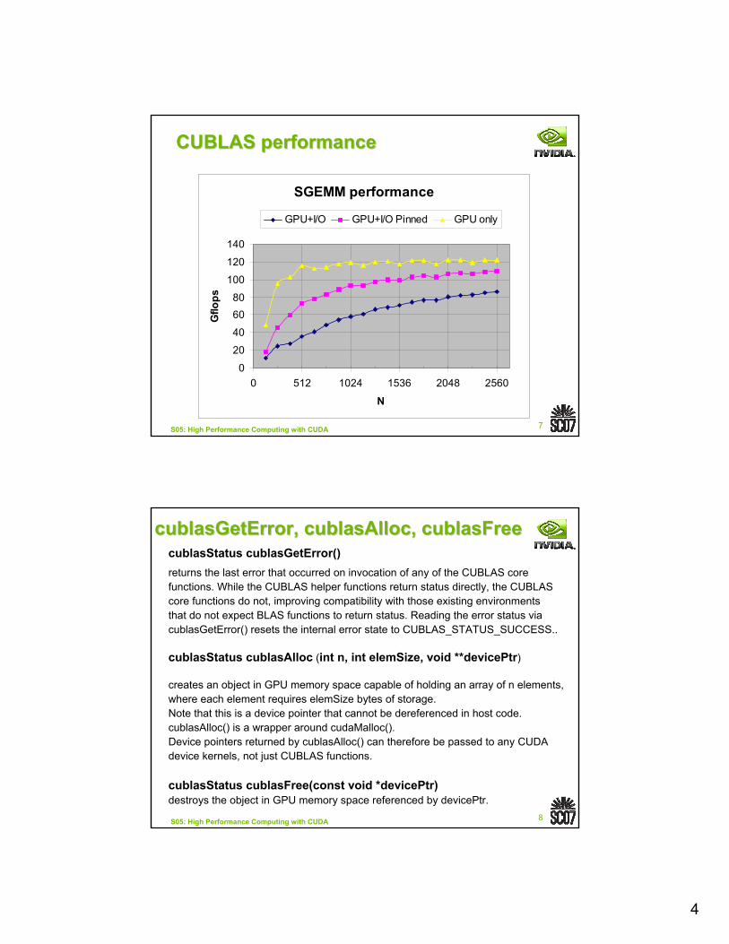
CUBLAS performanceCUBLAS performance
SGEMM performance
0
20
40
6080
100
120
140
0 512 1024 1536 2048 2560
N
Gflo
psGPU+I/O GPU+I/O Pinned GPU only
8S05: High Performance Computing with CUDA
cublasGetErrorcublasGetError, , cublasAlloccublasAlloc, , cublasFreecublasFreecublasStatus cublasGetError()returns the last error that occurred on invocation of any of the CUBLAS core functions. While the CUBLAS helper functions return status directly, the CUBLAScore functions do not, improving compatibility with those existing environmentsthat do not expect BLAS functions to return status. Reading the error status via cublasGetError() resets the internal error state to CUBLAS_STATUS_SUCCESS..
cublasStatus cublasAlloc (int n, int elemSize, void **devicePtr)
creates an object in GPU memory space capable of holding an array of n elements, where each element requires elemSize bytes of storage. Note that this is a device pointer that cannot be dereferenced in host code. cublasAlloc() is a wrapper around cudaMalloc(). Device pointers returned by cublasAlloc() can therefore be passed to any CUDA device kernels, not just CUBLAS functions.
cublasStatus cublasFree(const void *devicePtr)destroys the object in GPU memory space referenced by devicePtr.
5
9S05: High Performance Computing with CUDA
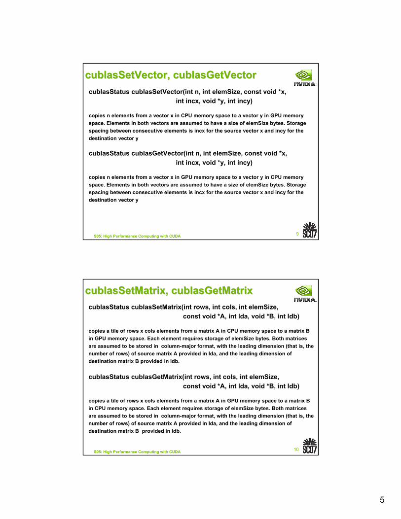
cublasSetVectorcublasSetVector, , cublasGetVectorcublasGetVectorcublasStatus cublasSetVector(int n, int elemSize, const void *x,
int incx, void *y, int incy)
copies n elements from a vector x in CPU memory space to a vector y in GPU memory space. Elements in both vectors are assumed to have a size of elemSize bytes. Storage spacing between consecutive elements is incx for the source vector x and incy for the destination vector y
cublasStatus cublasGetVector(int n, int elemSize, const void *x, int incx, void *y, int incy)
copies n elements from a vector x in GPU memory space to a vector y in CPU memory space. Elements in both vectors are assumed to have a size of elemSize bytes. Storage spacing between consecutive elements is incx for the source vector x and incy for the destination vector y
10S05: High Performance Computing with CUDA
cublasSetMatrixcublasSetMatrix, , cublasGetMatrixcublasGetMatrixcublasStatus cublasSetMatrix(int rows, int cols, int elemSize,
const void *A, int lda, void *B, int ldb)
copies a tile of rows x cols elements from a matrix A in CPU memory space to a matrix B in GPU memory space. Each element requires storage of elemSize bytes. Both matricesare assumed to be stored in column-major format, with the leading dimension (that is, the number of rows) of source matrix A provided in lda, and the leading dimension of destination matrix B provided in ldb.
cublasStatus cublasGetMatrix(int rows, int cols, int elemSize, const void *A, int lda, void *B, int ldb)
copies a tile of rows x cols elements from a matrix A in GPU memory space to a matrix B in CPU memory space. Each element requires storage of elemSize bytes. Both matrices are assumed to be stored in column-major format, with the leading dimension (that is, the number of rows) of source matrix A provided in lda, and the leading dimension of destination matrix B provided in ldb.
6
11S05: High Performance Computing with CUDA
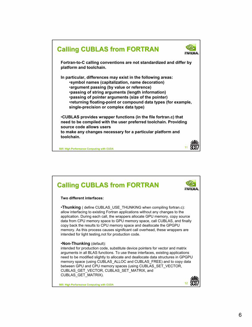
Calling CUBLAS from FORTRANCalling CUBLAS from FORTRAN
Fortran-to-C calling conventions are not standardized and differ by platform and toolchain.
In particular, differences may exist in the following areas:•symbol names (capitalization, name decoration)•argument passing (by value or reference)•passing of string arguments (length information)•passing of pointer arguments (size of the pointer)•returning floating-point or compound data types (for example, single-precision or complex data type)
•CUBLAS provides wrapper functions (in the file fortran.c) that need to be compiled with the user preferred toolchain. Providing source code allows users to make any changes necessary for a particular platform and toolchain.
12S05: High Performance Computing with CUDA
Calling CUBLAS from FORTRANCalling CUBLAS from FORTRAN
Two different interfaces:
•Thunking ( define CUBLAS_USE_THUNKING when compiling fortran.c):allow interfacing to existing Fortran applications without any changes to the application. During each call, the wrappers allocate GPU memory, copy source data from CPU memory space to GPU memory space, call CUBLAS, and finally copy back the results to CPU memory space and deallocate the GPGPU memory. As this process causes significant call overhead, these wrappers are intended for light testing,not for production code.
•Non-Thunking (default):intended for production code, substitute device pointers for vector and matrix arguments in all BLAS functions. To use these interfaces, existing applications need to be modified slightly to allocate and deallocate data structures in GPGPU memory space (using CUBLAS_ALLOC and CUBLAS_FREE) and to copy data between GPU and CPU memory spaces (using CUBLAS_SET_VECTOR, CUBLAS_GET_VECTOR, CUBLAS_SET_MATRIX, and CUBLAS_GET_MATRIX).
7
13S05: High Performance Computing with CUDA
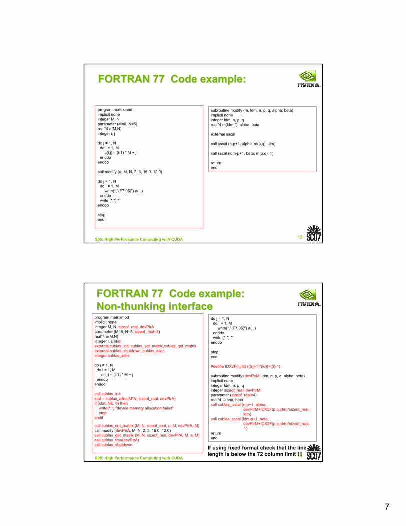
FORTRAN 77 Code example:FORTRAN 77 Code example:
program matrixmodimplicit noneinteger M, Nparameter (M=6, N=5)real*4 a(M,N)integer i, j
do j = 1, Ndo i = 1, M
a(i,j) = (i-1) * M + jenddo
enddo
call modify (a, M, N, 2, 3, 16.0, 12.0)
do j = 1, Ndo i = 1, M
write(*,"(F7.0$)") a(i,j)enddowrite (*,*) "”
enddo
stopend
subroutine modify (m, ldm, n, p, q, alpha, beta)implicit noneinteger ldm, n, p, qreal*4 m(ldm,*), alpha, beta
external sscal
call sscal (n-p+1, alpha, m(p,q), ldm)
call sscal (ldm-p+1, beta, m(p,q), 1)
returnend
14S05: High Performance Computing with CUDA
FORTRAN 77 Code example:FORTRAN 77 Code example:NonNon--thunkingthunking interfaceinterface
program matrixmodimplicit noneinteger M, N, sizeof_real, devPtrAparameter (M=6, N=5, sizeof_real=4)real*4 a(M,N)integer i, j, statexternal cublas_init, cublas_set_matrix,cublas_get_matrixexternal cublas_shutdown, cublas_allocinteger cublas_alloc
do j = 1, Ndo i = 1, M
a(i,j) = (i-1) * M + jenddo
enddo
call cublas_initstat = cublas_alloc(M*N, sizeof_real, devPtrA)if (stat .NE. 0) then
write(*,*) "device memory allocation failed"stop
endif
call cublas_set_matrix (M, N, sizeof_real, a, M, devPtrA, M)call modify (devPtrA, M, N, 2, 3, 16.0, 12.0)call cublas_get_matrix (M, N, sizeof_real, devPtrA, M, a, M)call cublas_free(devPtrA)call cublas_shutdown
do j = 1, Ndo i = 1, M
write(*,"(F7.0$)") a(i,j)enddowrite (*,*) "”
enddo
stopend
#define IDX2F(i,j,ld) ((((j)-1)*(ld))+((i)-1)
subroutine modify (devPtrM, ldm, n, p, q, alpha, beta)implicit noneinteger ldm, n, p, qinteger sizeof_real, devPtrMparameter (sizeof_real=4)real*4 alpha, betacall cublas_sscal (n-p+1, alpha,
devPtrM+IDX2F(p,q,ldm)*sizeof_real, ldm)
call cublas_sscal (ldm-p+1, beta, devPtrM+IDX2F(p,q,ldm)*sizeof_real, 1)
returnend
If using fixed format check that the linelength is below the 72 column limit !!!
8
15S05: High Performance Computing with CUDA
CUFFTCUFFTThe Fast Fourier Transform (FFT) is a divide-and-conquer algorithm for efficiently computing discrete Fourier transform of complex or real-valued data sets.
The FFT is one of the most important and widely used numerical algorithms.
CUFFT, the “CUDA” FFT library, provides a simple interface for computing parallel FFT on an NVIDIA GPU. This allows users to leverage the floating-point power and parallelism of the GPU without having to develop a custom, GPU-based FFT implementation.
16S05: High Performance Computing with CUDA
Supported featuresSupported features
• 1D, 2D and 3D transforms of complex and real-valued data• Batched execution for doing multiple 1D transforms in
parallel• 1D transform size up to 8M elements• 2D and 3D transform sizes in the range [2,16384]• In-place and out-of-place transforms for real and
complex data.
9
17S05: High Performance Computing with CUDA
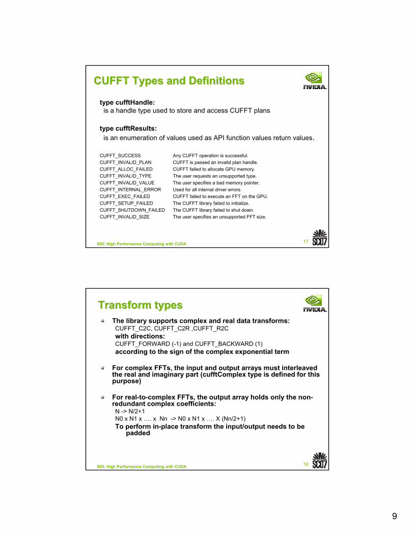
CUFFT Types and DefinitionsCUFFT Types and Definitions
type cufftHandle:is a handle type used to store and access CUFFT plans
type cufftResults:is an enumeration of values used as API function values return values.
CUFFT_SUCCESS Any CUFFT operation is successful.CUFFT_INVALID_PLAN CUFFT is passed an invalid plan handle.CUFFT_ALLOC_FAILED CUFFT failed to allocate GPU memory.CUFFT_INVALID_TYPE The user requests an unsupported type.CUFFT_INVALID_VALUE The user specifies a bad memory pointer.CUFFT_INTERNAL_ERROR Used for all internal driver errors.CUFFT_EXEC_FAILED CUFFT failed to execute an FFT on the GPU.CUFFT_SETUP_FAILED The CUFFT library failed to initialize.CUFFT_SHUTDOWN_FAILED The CUFFT library failed to shut down.CUFFT_INVALID_SIZE The user specifies an unsupported FFT size.
18S05: High Performance Computing with CUDA
Transform typesTransform typesThe library supports complex and real data transforms:CUFFT_C2C, CUFFT_C2R ,CUFFT_R2Cwith directions:CUFFT_FORWARD (-1) and CUFFT_BACKWARD (1)according to the sign of the complex exponential term
For complex FFTs, the input and output arrays must interleaved the real and imaginary part (cufftComplex type is defined for this purpose)
For real-to-complex FFTs, the output array holds only the non-redundant complex coefficients:N -> N/2+1N0 x N1 x …. x Nn -> N0 x N1 x …. X (Nn/2+1)To perform in-place transform the input/output needs to be
padded
10
19S05: High Performance Computing with CUDA
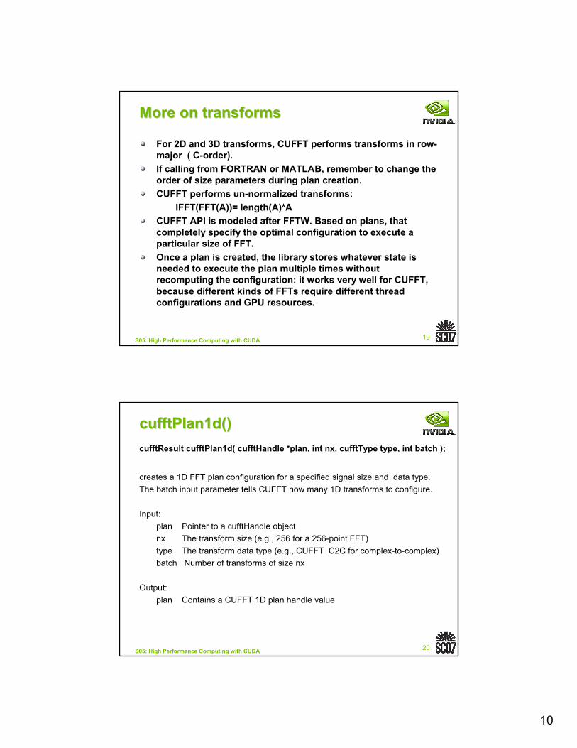
More on transformsMore on transforms
For 2D and 3D transforms, CUFFT performs transforms in row-major ( C-order).If calling from FORTRAN or MATLAB, remember to change the order of size parameters during plan creation.CUFFT performs un-normalized transforms:
IFFT(FFT(A))= length(A)*ACUFFT API is modeled after FFTW. Based on plans, that completely specify the optimal configuration to execute a particular size of FFT.Once a plan is created, the library stores whatever state is needed to execute the plan multiple times without recomputing the configuration: it works very well for CUFFT, because different kinds of FFTs require different thread configurations and GPU resources.
20S05: High Performance Computing with CUDA
cufftPlan1d()cufftPlan1d()cufftResult cufftPlan1d( cufftHandle *plan, int nx, cufftType type, int batch );
creates a 1D FFT plan configuration for a specified signal size and data type. The batch input parameter tells CUFFT how many 1D transforms to configure.
Input:plan Pointer to a cufftHandle objectnx The transform size (e.g., 256 for a 256-point FFT)type The transform data type (e.g., CUFFT_C2C for complex-to-complex)batch Number of transforms of size nx
Output:plan Contains a CUFFT 1D plan handle value
11
21S05: High Performance Computing with CUDA
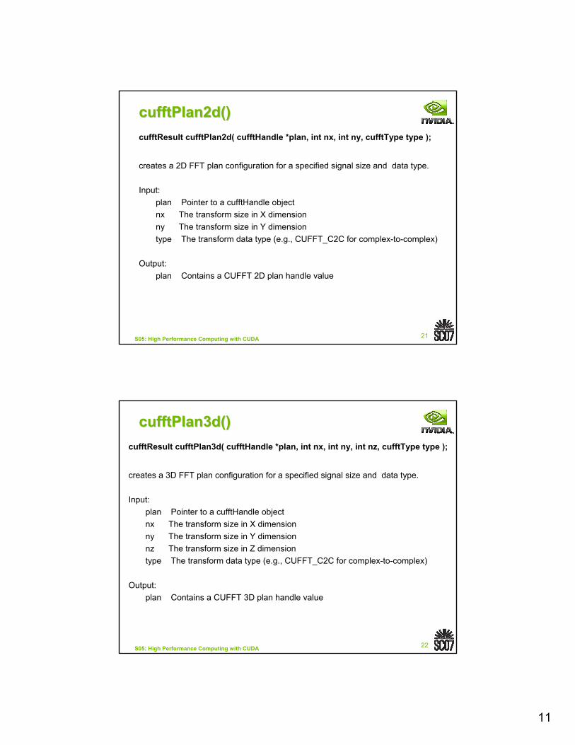
cufftPlan2d()cufftPlan2d()cufftResult cufftPlan2d( cufftHandle *plan, int nx, int ny, cufftType type );
creates a 2D FFT plan configuration for a specified signal size and data type.
Input:plan Pointer to a cufftHandle objectnx The transform size in X dimensionny The transform size in Y dimensiontype The transform data type (e.g., CUFFT_C2C for complex-to-complex)
Output:plan Contains a CUFFT 2D plan handle value
22S05: High Performance Computing with CUDA
cufftPlan3d()cufftPlan3d()cufftResult cufftPlan3d( cufftHandle *plan, int nx, int ny, int nz, cufftType type );
creates a 3D FFT plan configuration for a specified signal size and data type.
Input:plan Pointer to a cufftHandle objectnx The transform size in X dimensionny The transform size in Y dimensionnz The transform size in Z dimensiontype The transform data type (e.g., CUFFT_C2C for complex-to-complex)
Output:plan Contains a CUFFT 3D plan handle value
12
23S05: High Performance Computing with CUDA
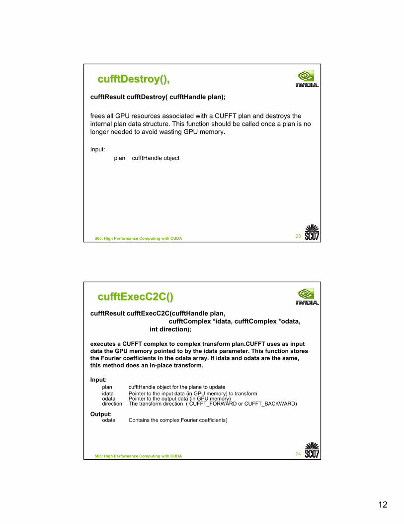
cufftDestroycufftDestroy(), (), cufftResult cufftDestroy( cufftHandle plan);
frees all GPU resources associated with a CUFFT plan and destroys the internal plan data structure. This function should be called once a plan is no longer needed to avoid wasting GPU memory.
Input:plan cufftHandle object
24S05: High Performance Computing with CUDA
cufftExecC2C()cufftExecC2C()cufftResult cufftExecC2C(cufftHandle plan,
cufftComplex *idata, cufftComplex *odata, int direction);
executes a CUFFT complex to complex transform plan.CUFFT uses as input data the GPU memory pointed to by the idata parameter. This function stores the Fourier coefficients in the odata array. If idata and odata are the same, this method does an in-place transform.
Input:plan cufftHandle object for the plane to updateidata Pointer to the input data (in GPU memory) to transformodata Pointer to the output data (in GPU memory) direction The transform direction ( CUFFT_FORWARD or CUFFT_BACKWARD)
Output:odata Contains the complex Fourier coefficients)
13
25S05: High Performance Computing with CUDA
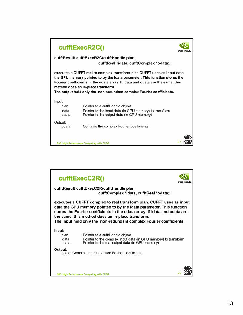
cufftExecR2C()cufftExecR2C()cufftResult cufftExecR2C(cufftHandle plan,
cufftReal *idata, cufftComplex *odata);
executes a CUFFT real to complex transform plan.CUFFT uses as input datathe GPU memory pointed to by the idata parameter. This function stores the Fourier coefficients in the odata array. If idata and odata are the same, this method does an in-place transform. The output hold only the non-redundant complex Fourier coefficients.
Input:plan Pointer to a cufftHandle objectidata Pointer to the input data (in GPU memory) to transformodata Pointer to the output data (in GPU memory)
Output:odata Contains the complex Fourier coefficients
26S05: High Performance Computing with CUDA
cufftExecC2R()cufftExecC2R()cufftResult cufftExecC2R(cufftHandle plan,
cufftComplex *idata, cufftReal *odata);
executes a CUFFT complex to real transform plan. CUFFT uses as inputdata the GPU memory pointed to by the idata parameter. This function stores the Fourier coefficients in the odata array. If idata and odata are the same, this method does an in-place transform.The input hold only the non-redundant complex Fourier coefficients.
Input:plan Pointer to a cufftHandle objectidata Pointer to the complex input data (in GPU memory) to transformodata Pointer to the real output data (in GPU memory)
Output:odata Contains the real-valued Fourier coefficients
14
27S05: High Performance Computing with CUDA
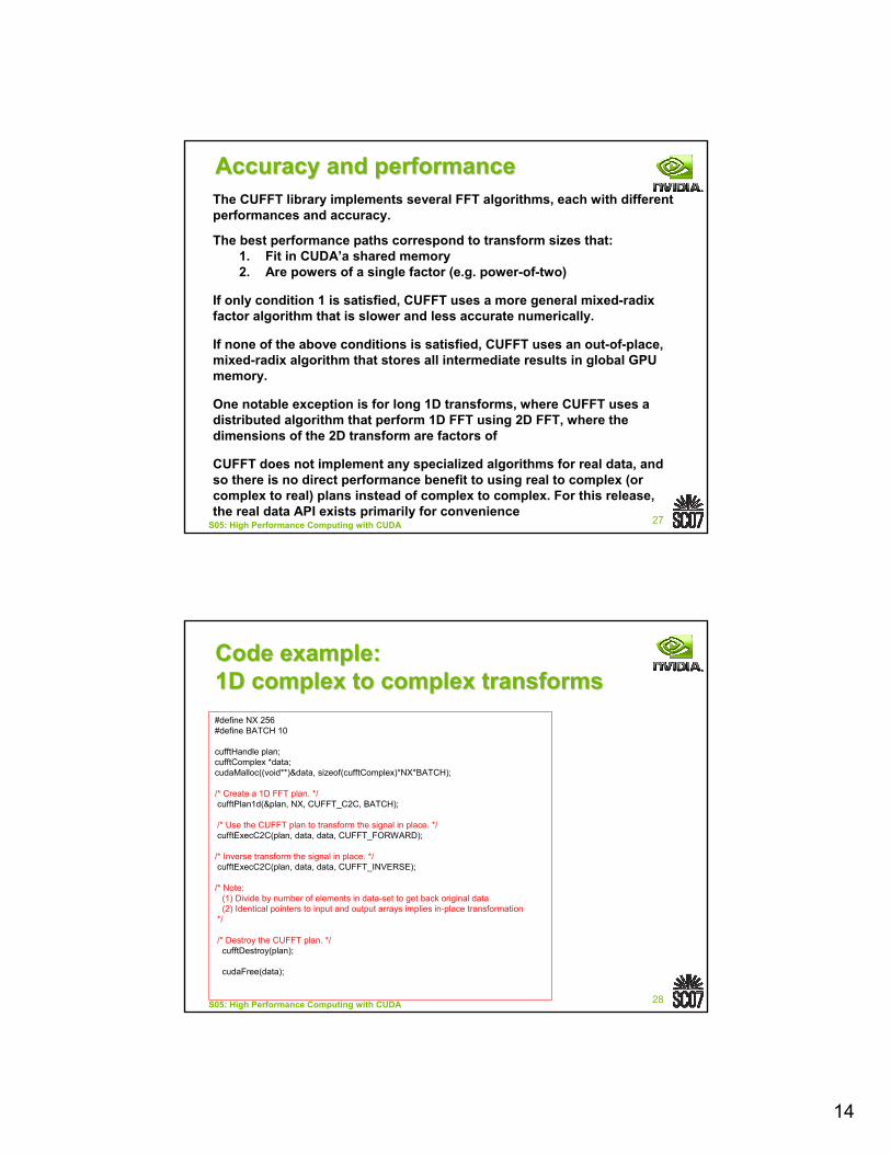
Accuracy and performanceAccuracy and performanceThe CUFFT library implements several FFT algorithms, each with differentperformances and accuracy.
The best performance paths correspond to transform sizes that:1. Fit in CUDA’a shared memory2. Are powers of a single factor (e.g. power-of-two)
If only condition 1 is satisfied, CUFFT uses a more general mixed-radix factor algorithm that is slower and less accurate numerically.
If none of the above conditions is satisfied, CUFFT uses an out-of-place, mixed-radix algorithm that stores all intermediate results in global GPU memory.
One notable exception is for long 1D transforms, where CUFFT uses a distributed algorithm that perform 1D FFT using 2D FFT, where the dimensions of the 2D transform are factors of
CUFFT does not implement any specialized algorithms for real data, and so there is no direct performance benefit to using real to complex (or complex to real) plans instead of complex to complex. For this release, the real data API exists primarily for convenience
28S05: High Performance Computing with CUDA
Code example:Code example:1D complex to complex transforms1D complex to complex transforms#define NX 256#define BATCH 10
cufftHandle plan;cufftComplex *data;cudaMalloc((void**)&data, sizeof(cufftComplex)*NX*BATCH);
/* Create a 1D FFT plan. */cufftPlan1d(&plan, NX, CUFFT_C2C, BATCH);
/* Use the CUFFT plan to transform the signal in place. */cufftExecC2C(plan, data, data, CUFFT_FORWARD);
/* Inverse transform the signal in place. */cufftExecC2C(plan, data, data, CUFFT_INVERSE);
/* Note:(1) Divide by number of elements in data-set to get back original data(2) Identical pointers to input and output arrays implies in-place transformation
*/
/* Destroy the CUFFT plan. */cufftDestroy(plan);
cudaFree(data);
15
29S05: High Performance Computing with CUDA
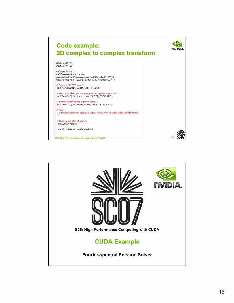
Code example:Code example:2D complex to complex transform2D complex to complex transform#define NX 256#define NY 128
cufftHandle plan;cufftComplex *idata, *odata;cudaMalloc((void**)&idata, sizeof(cufftComplex)*NX*NY);cudaMalloc((void**)&odata, sizeof(cufftComplex)*NX*NY);
/* Create a 1D FFT plan. */cufftPlan2d(&plan, NX,NY, CUFFT_C2C);
/* Use the CUFFT plan to transform the signal out of place. */cufftExecC2C(plan, idata, odata, CUFFT_FORWARD);
/* Inverse transform the signal in place. */cufftExecC2C(plan, odata, odata, CUFFT_INVERSE);
/* Note:Different pointers to input and output arrays implies out of place transformation
*/
/* Destroy the CUFFT plan. */cufftDestroy(plan);
cudaFree(idata), cudaFree(odata);
S05: High Performance Computing with CUDA
CUDA ExampleCUDA Example
Fourier-spectral Poisson Solver
16
31S05: High Performance Computing with CUDA
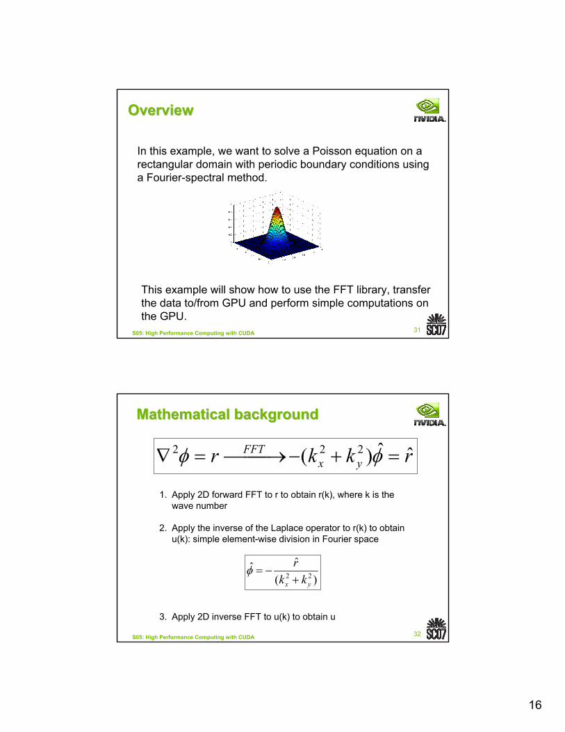
OverviewOverview
In this example, we want to solve a Poisson equation on a rectangular domain with periodic boundary conditions using a Fourier-spectral method.
This example will show how to use the FFT library, transfer the data to/from GPU and perform simple computations on the GPU.
32S05: High Performance Computing with CUDA
Mathematical backgroundMathematical background
rkkr yxFFT ˆˆ)( 222 =+−⎯⎯→⎯=∇ φφ
1. Apply 2D forward FFT to r to obtain r(k), where k is the wave number
2. Apply the inverse of the Laplace operator to r(k) to obtain u(k): simple element-wise division in Fourier space
3. Apply 2D inverse FFT to u(k) to obtain u
)(ˆˆ
22yx kk
r+
−=φ
17
33S05: High Performance Computing with CUDA
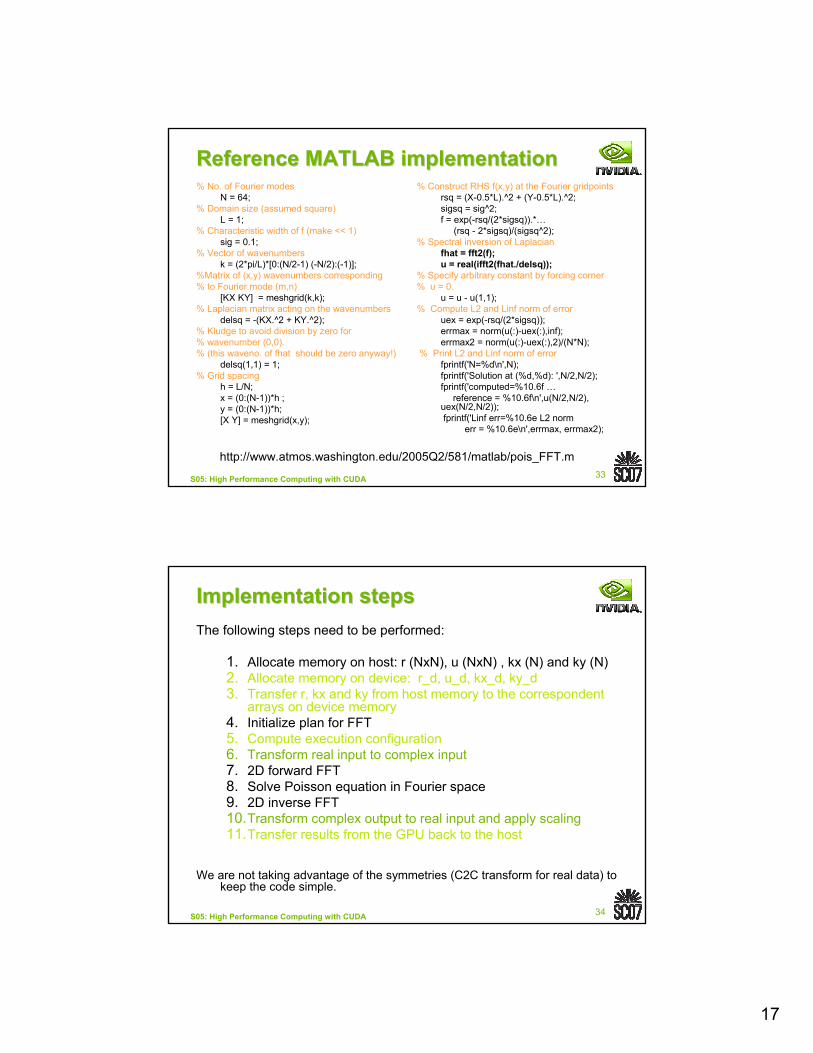
Reference MATLAB implementationReference MATLAB implementation% No. of Fourier modes
N = 64; % Domain size (assumed square)
L = 1; % Characteristic width of f (make << 1)
sig = 0.1; % Vector of wavenumbers
k = (2*pi/L)*[0:(N/2-1) (-N/2):(-1)]; %Matrix of (x,y) wavenumbers corresponding% to Fourier mode (m,n)
[KX KY] = meshgrid(k,k);% Laplacian matrix acting on the wavenumbers
delsq = -(KX.^2 + KY.^2);% Kludge to avoid division by zero for% wavenumber (0,0).% (this waveno. of fhat should be zero anyway!)
delsq(1,1) = 1; % Grid spacing
h = L/N; x = (0:(N-1))*h ;y = (0:(N-1))*h;[X Y] = meshgrid(x,y);
% Construct RHS f(x,y) at the Fourier gridpointsrsq = (X-0.5*L).^2 + (Y-0.5*L).^2;sigsq = sig^2;f = exp(-rsq/(2*sigsq)).*…
(rsq - 2*sigsq)/(sigsq^2);% Spectral inversion of Laplacian
fhat = fft2(f);u = real(ifft2(fhat./delsq));
% Specify arbitrary constant by forcing corner% u = 0.
u = u - u(1,1); % Compute L2 and Linf norm of error
uex = exp(-rsq/(2*sigsq));errmax = norm(u(:)-uex(:),inf);errmax2 = norm(u(:)-uex(:),2)/(N*N);
% Print L2 and Linf norm of errorfprintf('N=%d\n',N);fprintf('Solution at (%d,%d): ',N/2,N/2);fprintf('computed=%10.6f …
reference = %10.6f\n',u(N/2,N/2), uex(N/2,N/2));fprintf('Linf err=%10.6e L2 norm
err = %10.6e\n',errmax, errmax2);
http://www.atmos.washington.edu/2005Q2/581/matlab/pois_FFT.m
34S05: High Performance Computing with CUDA
Implementation stepsImplementation stepsThe following steps need to be performed:
1. Allocate memory on host: r (NxN), u (NxN) , kx (N) and ky (N)2. Allocate memory on device: r_d, u_d, kx_d, ky_d3. Transfer r, kx and ky from host memory to the correspondent
arrays on device memory4. Initialize plan for FFT5. Compute execution configuration6. Transform real input to complex input7. 2D forward FFT8. Solve Poisson equation in Fourier space9. 2D inverse FFT10.Transform complex output to real input and apply scaling11.Transfer results from the GPU back to the host
We are not taking advantage of the symmetries (C2C transform for real data) to keep the code simple.
18
35S05: High Performance Computing with CUDA
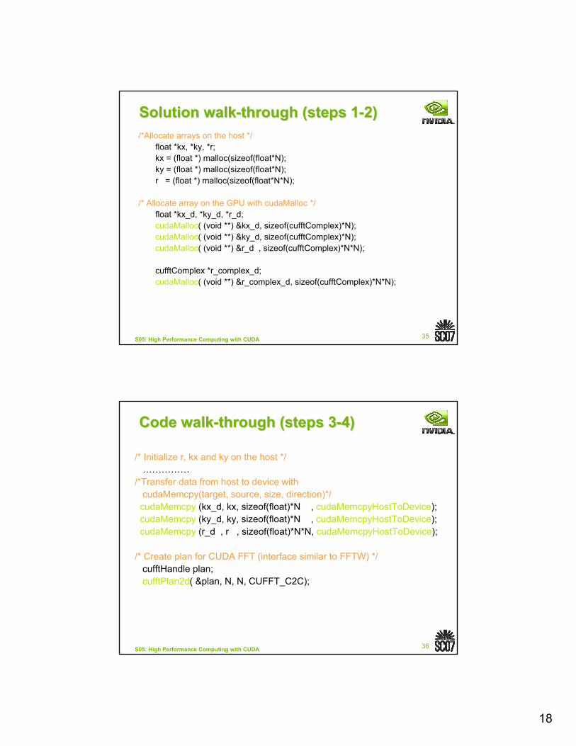
Solution walkSolution walk--through (steps 1through (steps 1--2)2)/*Allocate arrays on the host */
float *kx, *ky, *r;kx = (float *) malloc(sizeof(float*N);ky = (float *) malloc(sizeof(float*N);r = (float *) malloc(sizeof(float*N*N);
/* Allocate array on the GPU with cudaMalloc */float *kx_d, *ky_d, *r_d;cudaMalloc( (void **) &kx_d, sizeof(cufftComplex)*N);cudaMalloc( (void **) &ky_d, sizeof(cufftComplex)*N);cudaMalloc( (void **) &r_d , sizeof(cufftComplex)*N*N);
cufftComplex *r_complex_d;cudaMalloc( (void **) &r_complex_d, sizeof(cufftComplex)*N*N);
36S05: High Performance Computing with CUDA
Code walkCode walk--through (steps 3through (steps 3--4)4)
/* Initialize r, kx and ky on the host */……………
/*Transfer data from host to device with cudaMemcpy(target, source, size, direction)*/cudaMemcpy (kx_d, kx, sizeof(float)*N , cudaMemcpyHostToDevice);cudaMemcpy (ky_d, ky, sizeof(float)*N , cudaMemcpyHostToDevice);cudaMemcpy (r_d , r , sizeof(float)*N*N, cudaMemcpyHostToDevice);
/* Create plan for CUDA FFT (interface similar to FFTW) */cufftHandle plan;cufftPlan2d( &plan, N, N, CUFFT_C2C);
19
37S05: High Performance Computing with CUDA
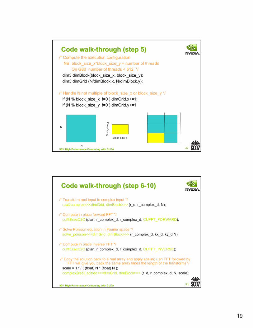
Code walkCode walk--through (step 5)through (step 5)/* Compute the execution configuration
NB: block_size_x*block_size_y = number of threadsOn G80 number of threads < 512 */
dim3 dimBlock(block_size_x, block_size_y);dim3 dimGrid (N/dimBlock.x, N/dimBlock.y);
/* Handle N not multiple of block_size_x or block_size_y */if (N % block_size_x !=0 ) dimGrid.x+=1; if (N % block_size_y !=0 ) dimGrid.y+=1
Block_size_x
Blo
ck_s
ize_
y
N
N
38S05: High Performance Computing with CUDA
Code walkCode walk--through (step 6through (step 6--10)10)
/* Transform real input to complex input */real2complex<<<dimGrid, dimBlock>>> (r_d, r_complex_d, N);
/* Compute in place forward FFT */cufftExecC2C (plan, r_complex_d, r_complex_d, CUFFT_FORWARD);
/* Solve Poisson equation in Fourier space */solve_poisson<<<dimGrid, dimBlock>>> (r_complex_d, kx_d, ky_d,N);
/* Compute in place inverse FFT */cufftExecC2C (plan, r_complex_d, r_complex_d, CUFFT_INVERSE);
/* Copy the solution back to a real array and apply scaling ( an FFT followed by iFFT will give you back the same array times the length of the transform) */
scale = 1.f / ( (float) N * (float) N );complex2real_scaled<<<dimGrid, dimBlock>>> (r_d, r_complex_d, N, scale);
20
39S05: High Performance Computing with CUDA
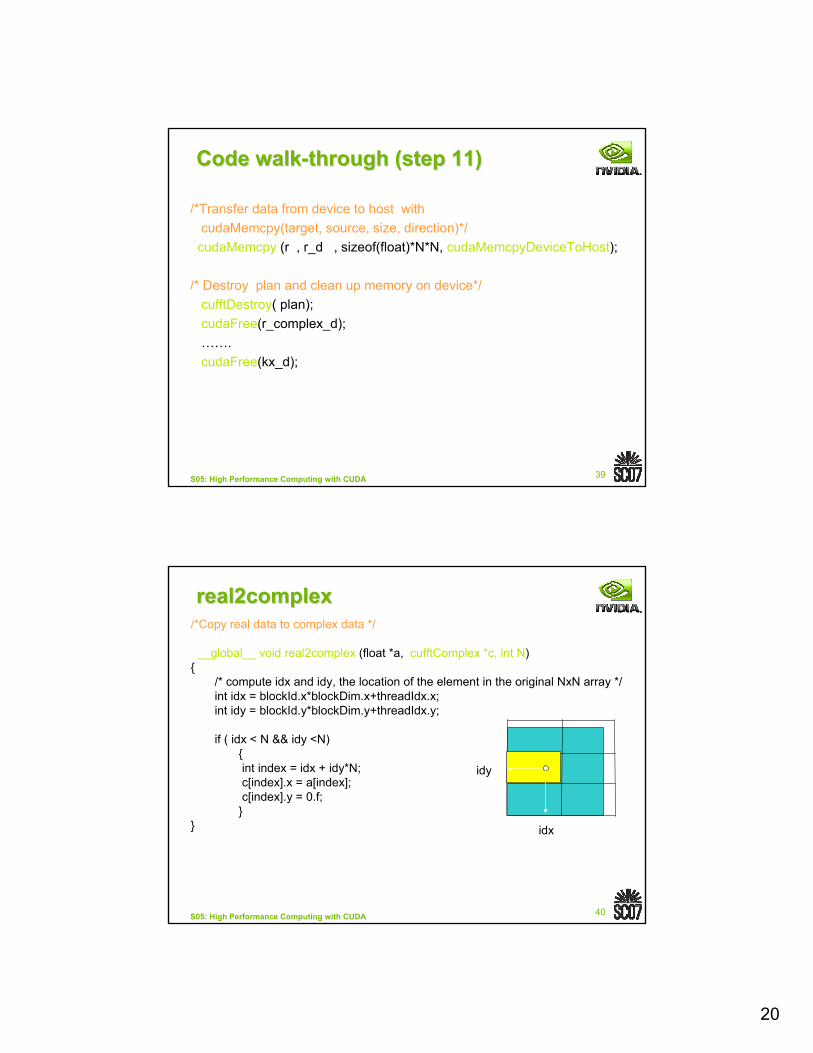
Code walkCode walk--through (step 11)through (step 11)
/*Transfer data from device to host with cudaMemcpy(target, source, size, direction)*/cudaMemcpy (r , r_d , sizeof(float)*N*N, cudaMemcpyDeviceToHost);
/* Destroy plan and clean up memory on device*/cufftDestroy( plan);cudaFree(r_complex_d); ……. cudaFree(kx_d);
40S05: High Performance Computing with CUDA
real2complexreal2complex/*Copy real data to complex data */
__global__ void real2complex (float *a, cufftComplex *c, int N){
/* compute idx and idy, the location of the element in the original NxN array */int idx = blockId.x*blockDim.x+threadIdx.x;int idy = blockId.y*blockDim.y+threadIdx.y;
if ( idx < N && idy <N){int index = idx + idy*N;c[index].x = a[index];c[index].y = 0.f;
}} idx
idy
21
41S05: High Performance Computing with CUDA
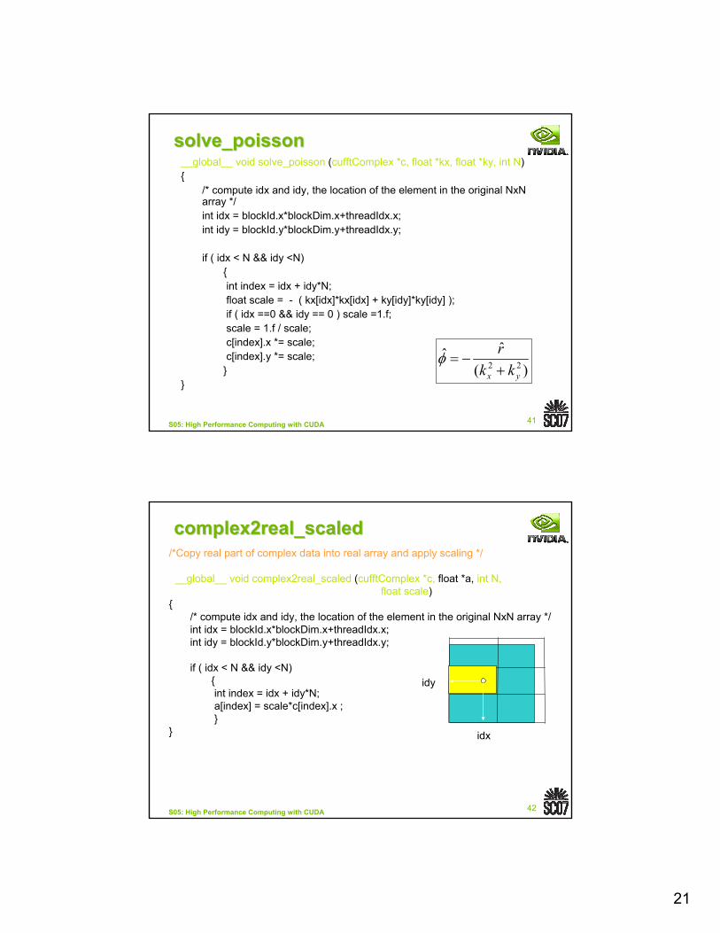
solve_poissonsolve_poisson__global__ void solve_poisson (cufftComplex *c, float *kx, float *ky, int N){
/* compute idx and idy, the location of the element in the original NxNarray */int idx = blockId.x*blockDim.x+threadIdx.x;int idy = blockId.y*blockDim.y+threadIdx.y;
if ( idx < N && idy <N){int index = idx + idy*N;float scale = - ( kx[idx]*kx[idx] + ky[idy]*ky[idy] );if ( idx ==0 && idy == 0 ) scale =1.f; scale = 1.f / scale;c[index].x *= scale;c[index].y *= scale;
}}
)(ˆˆ
22yx kk
r+
−=φ
42S05: High Performance Computing with CUDA
complex2real_scaledcomplex2real_scaled/*Copy real part of complex data into real array and apply scaling */
__global__ void complex2real_scaled (cufftComplex *c, float *a, int N, float scale)
{/* compute idx and idy, the location of the element in the original NxN array */int idx = blockId.x*blockDim.x+threadIdx.x;int idy = blockId.y*blockDim.y+threadIdx.y;
if ( idx < N && idy <N){int index = idx + idy*N;a[index] = scale*c[index].x ;}
} idx
idy
22
43S05: High Performance Computing with CUDA
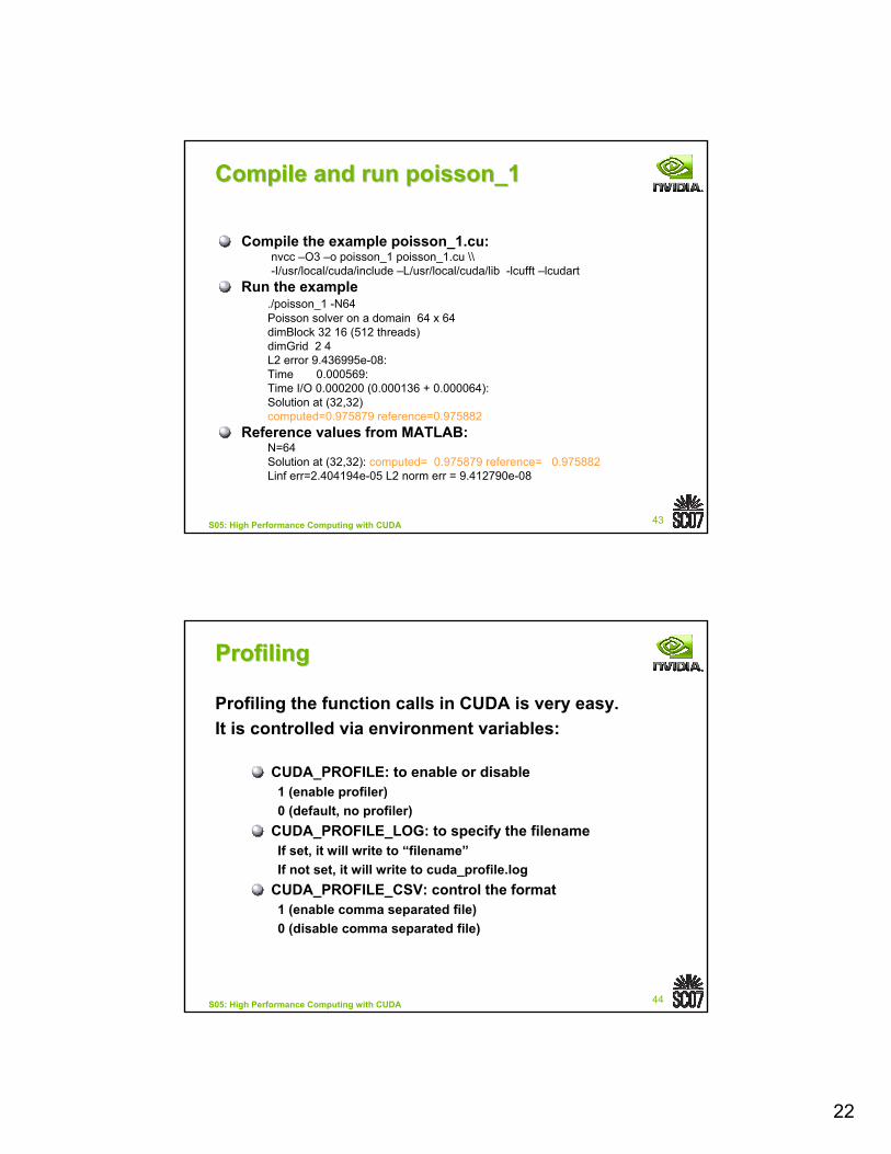
Compile and run poisson_1Compile and run poisson_1
Compile the example poisson_1.cu:nvcc –O3 –o poisson_1 poisson_1.cu \\-I/usr/local/cuda/include –L/usr/local/cuda/lib -lcufft –lcudart
Run the example./poisson_1 -N64Poisson solver on a domain 64 x 64dimBlock 32 16 (512 threads)dimGrid 2 4L2 error 9.436995e-08:Time 0.000569:Time I/O 0.000200 (0.000136 + 0.000064):Solution at (32,32)computed=0.975879 reference=0.975882
Reference values from MATLAB:N=64Solution at (32,32): computed= 0.975879 reference= 0.975882Linf err=2.404194e-05 L2 norm err = 9.412790e-08
44S05: High Performance Computing with CUDA
ProfilingProfiling
Profiling the function calls in CUDA is very easy. It is controlled via environment variables:
CUDA_PROFILE: to enable or disable1 (enable profiler)0 (default, no profiler)
CUDA_PROFILE_LOG: to specify the filenameIf set, it will write to “filename”If not set, it will write to cuda_profile.log
CUDA_PROFILE_CSV: control the format1 (enable comma separated file)0 (disable comma separated file)
23
45S05: High Performance Computing with CUDA
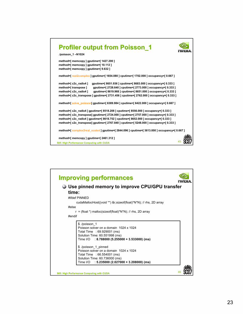
Profiler output from Poisson_1Profiler output from Poisson_1./poisson_1 –N1024
method=[ memcopy ] gputime=[ 1427.200 ]method=[ memcopy ] gputime=[ 10.112 ]method=[ memcopy ] gputime=[ 9.632 ]
method=[ real2complex ] gputime=[ 1654.080 ] cputime=[ 1702.000 ] occupancy=[ 0.667 ]
method=[ c2c_radix4 ] gputime=[ 8651.936 ] cputime=[ 8683.000 ] occupancy=[ 0.333 ]method=[ transpose ] gputime=[ 2728.640 ] cputime=[ 2773.000 ] occupancy=[ 0.333 ]method=[ c2c_radix4 ] gputime=[ 8619.968 ] cputime=[ 8651.000 ] occupancy=[ 0.333 ]method=[ c2c_transpose ] gputime=[ 2731.456 ] cputime=[ 2762.000 ] occupancy=[ 0.333 ]
method=[ solve_poisson] gputime=[ 6389.984 ] cputime=[ 6422.000 ] occupancy=[ 0.667 ]
method=[ c2c_radix4 ] gputime=[ 8518.208 ] cputime=[ 8556.000 ] occupancy=[ 0.333 ]method=[ c2c_transpose] gputime=[ 2724.000 ] cputime=[ 2757.000 ] occupancy=[ 0.333 ]method=[ c2c_radix4 ] gputime=[ 8618.752 ] cputime=[ 8652.000 ] occupancy=[ 0.333 ]method=[ c2c_transpose] gputime=[ 2767.840 ] cputime=[ 5248.000 ] occupancy=[ 0.333 ]
method=[ complex2real_scaled ] gputime=[ 2844.096 ] cputime=[ 3613.000 ] occupancy=[ 0.667 ]
method=[ memcopy ] gputime=[ 2461.312 ]
46S05: High Performance Computing with CUDA
Improving performancesImproving performancesUse pinned memory to improve CPU/GPU transfer time:#ifdef PINNED
cudaMallocHost((void **) &r,sizeof(float)*N*N); // rhs, 2D array#else
r = (float *) malloc(sizeof(float)*N*N); // rhs, 2D array#endif
$ ./poisson_1Poisson solver on a domain 1024 x 1024Total Time : 69.929001 (ms)Solution Time: 60.551998 (ms)Time I/O : 8.788000 (5.255000 + 3.533000) (ms)
$ ./poisson_1_pinned Poisson solver on a domain 1024 x 1024Total Time : 66.554001 (ms)Solution Time: 60.736000 (ms)Time I/O : 5.235000 (2.027000 + 3.208000) (ms)
24
47S05: High Performance Computing with CUDA
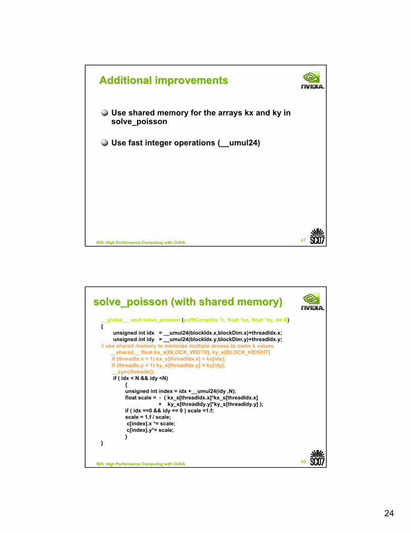
Additional improvementsAdditional improvements
Use shared memory for the arrays kx and ky in solve_poisson
Use fast integer operations (__umul24)
48S05: High Performance Computing with CUDA
solve_poissonsolve_poisson (with shared memory)(with shared memory)__global__ void solve_poisson (cufftComplex *c, float *kx, float *ky, int N){
unsigned int idx = __umul24(blockIdx.x,blockDim.x)+threadIdx.x;unsigned int idy = __umul24(blockIdx.y,blockDim.y)+threadIdx.y;
// use shared memory to minimize multiple access to same k values__shared__ float kx_s[BLOCK_WIDTH], ky_s[BLOCK_HEIGHT]if (threadIx.x < 1) kx_s[threadIdx.x] = kx[idx];if (threadIx.y < 1) ky_s[threadIdx.y] = ky[idy];__syncthreads();if ( idx < N && idy <N)
{unsigned int index = idx +__umul24(idy ,N);float scale = - ( kx_s[threadIdx.x]*kx_s[threadIdx.x]
+ ky_s[threadIdy.y]*ky_s[threadIdy.y] );if ( idx ==0 && idy == 0 ) scale =1.f; scale = 1.f / scale;c[index].x *= scale;c[index].y*= scale;
}}
25
49S05: High Performance Computing with CUDA
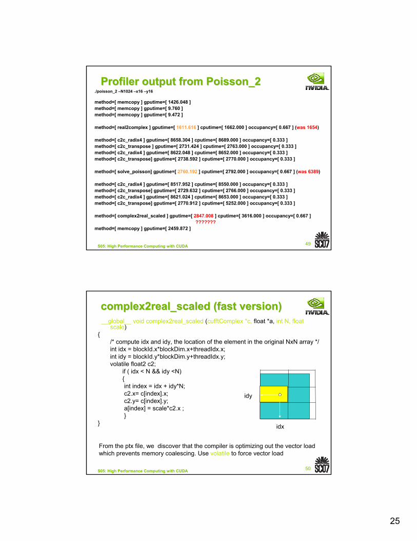
Profiler output from Poisson_2Profiler output from Poisson_2./poisson_2 –N1024 –x16 –y16
method=[ memcopy ] gputime=[ 1426.048 ]method=[ memcopy ] gputime=[ 9.760 ]method=[ memcopy ] gputime=[ 9.472 ]
method=[ real2complex ] gputime=[ 1611.616 ] cputime=[ 1662.000 ] occupancy=[ 0.667 ] (was 1654)
method=[ c2c_radix4 ] gputime=[ 8658.304 ] cputime=[ 8689.000 ] occupancy=[ 0.333 ]method=[ c2c_transpose ] gputime=[ 2731.424 ] cputime=[ 2763.000 ] occupancy=[ 0.333 ]method=[ c2c_radix4 ] gputime=[ 8622.048 ] cputime=[ 8652.000 ] occupancy=[ 0.333 ]method=[ c2c_transpose] gputime=[ 2738.592 ] cputime=[ 2770.000 ] occupancy=[ 0.333 ]
method=[ solve_poisson] gputime=[ 2760.192 ] cputime=[ 2792.000 ] occupancy=[ 0.667 ] (was 6389)
method=[ c2c_radix4 ] gputime=[ 8517.952 ] cputime=[ 8550.000 ] occupancy=[ 0.333 ]method=[ c2c_transpose] gputime=[ 2729.632 ] cputime=[ 2766.000 ] occupancy=[ 0.333 ]method=[ c2c_radix4 ] gputime=[ 8621.024 ] cputime=[ 8653.000 ] occupancy=[ 0.333 ]method=[ c2c_transpose] gputime=[ 2770.912 ] cputime=[ 5252.000 ] occupancy=[ 0.333 ]
method=[ complex2real_scaled ] gputime=[ 2847.008 ] cputime=[ 3616.000 ] occupancy=[ 0.667 ]???????
method=[ memcopy ] gputime=[ 2459.872 ]
50S05: High Performance Computing with CUDA
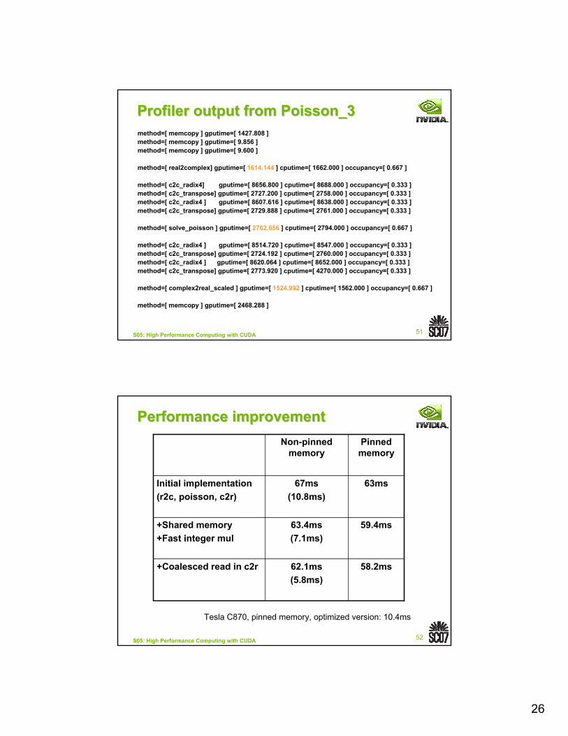
complex2real_scaled (fast version)complex2real_scaled (fast version)__global__ void complex2real_scaled (cufftComplex *c, float *a, int N, float
scale){
/* compute idx and idy, the location of the element in the original NxN array */int idx = blockId.x*blockDim.x+threadIdx.x;int idy = blockId.y*blockDim.y+threadIdx.y;volatile float2 c2;
if ( idx < N && idy <N){int index = idx + idy*N;c2.x= c[index].x;c2.y= c[index].y;a[index] = scale*c2.x ;}
} idx
idy
From the ptx file, we discover that the compiler is optimizing out the vector load which prevents memory coalescing. Use volatile to force vector load
26
51S05: High Performance Computing with CUDA
Profiler output from Poisson_3Profiler output from Poisson_3method=[ memcopy ] gputime=[ 1427.808 ]method=[ memcopy ] gputime=[ 9.856 ]method=[ memcopy ] gputime=[ 9.600 ]
method=[ real2complex] gputime=[ 1614.144 ] cputime=[ 1662.000 ] occupancy=[ 0.667 ]
method=[ c2c_radix4] gputime=[ 8656.800 ] cputime=[ 8688.000 ] occupancy=[ 0.333 ]method=[ c2c_transpose] gputime=[ 2727.200 ] cputime=[ 2758.000 ] occupancy=[ 0.333 ]method=[ c2c_radix4 ] gputime=[ 8607.616 ] cputime=[ 8638.000 ] occupancy=[ 0.333 ]method=[ c2c_transpose] gputime=[ 2729.888 ] cputime=[ 2761.000 ] occupancy=[ 0.333 ]
method=[ solve_poisson ] gputime=[ 2762.656 ] cputime=[ 2794.000 ] occupancy=[ 0.667 ]
method=[ c2c_radix4 ] gputime=[ 8514.720 ] cputime=[ 8547.000 ] occupancy=[ 0.333 ]method=[ c2c_transpose] gputime=[ 2724.192 ] cputime=[ 2760.000 ] occupancy=[ 0.333 ]method=[ c2c_radix4 ] gputime=[ 8620.064 ] cputime=[ 8652.000 ] occupancy=[ 0.333 ]method=[ c2c_transpose] gputime=[ 2773.920 ] cputime=[ 4270.000 ] occupancy=[ 0.333 ]
method=[ complex2real_scaled ] gputime=[ 1524.992 ] cputime=[ 1562.000 ] occupancy=[ 0.667 ]
method=[ memcopy ] gputime=[ 2468.288 ]
52S05: High Performance Computing with CUDA
Performance improvementPerformance improvement
63ms67ms(10.8ms)
Initial implementation(r2c, poisson, c2r)
58.2ms62.1ms(5.8ms)
+Coalesced read in c2r
59.4ms63.4ms(7.1ms)
+Shared memory+Fast integer mul
Pinned memory
Non-pinned memory
Tesla C870, pinned memory, optimized version: 10.4ms
27
S05: High Performance Computing with CUDA
Accelerating MATLAB with CUDAAccelerating MATLAB with CUDA
54S05: High Performance Computing with CUDA
OverviewOverview
MATLAB can be easily extended via MEX files to take advantage of the computational power offered by the latest NVIDIA GPUs (GeForce 8800, Quadro FX5600, Tesla).
Programming the GPU for computational purposes was a very cumbersome task before CUDA. Using CUDA, it is now very easy to achieve impressive speed-up with minimal effort.
28
55S05: High Performance Computing with CUDA
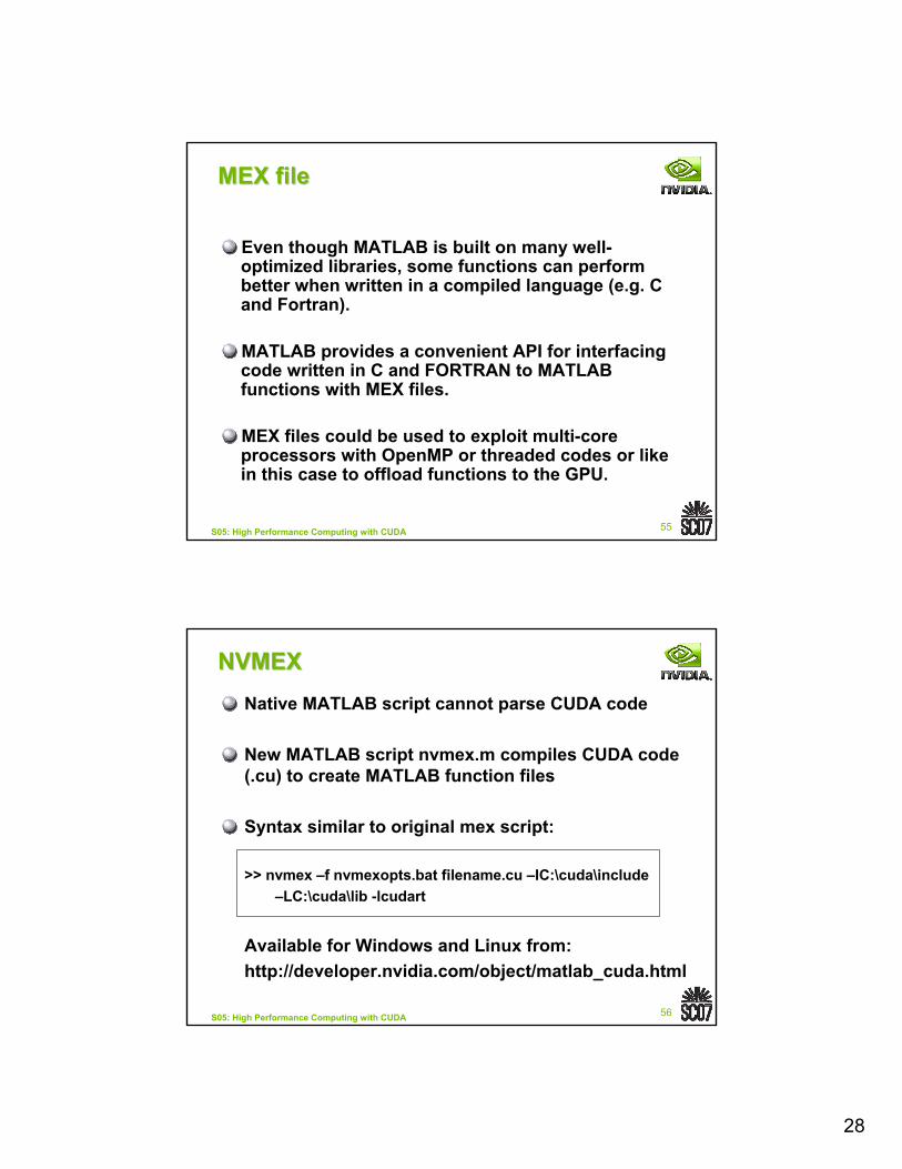
MEX fileMEX file
Even though MATLAB is built on many well-optimized libraries, some functions can perform better when written in a compiled language (e.g. C and Fortran).
MATLAB provides a convenient API for interfacing code written in C and FORTRAN to MATLAB functions with MEX files.
MEX files could be used to exploit multi-core processors with OpenMP or threaded codes or like in this case to offload functions to the GPU.
56S05: High Performance Computing with CUDA
NVMEX NVMEX Native MATLAB script cannot parse CUDA code
New MATLAB script nvmex.m compiles CUDA code (.cu) to create MATLAB function files
Syntax similar to original mex script:
>> nvmex –f nvmexopts.bat filename.cu –IC:\cuda\include–LC:\cuda\lib -lcudart
Available for Windows and Linux from:http://developer.nvidia.com/object/matlab_cuda.html
29
57S05: High Performance Computing with CUDA
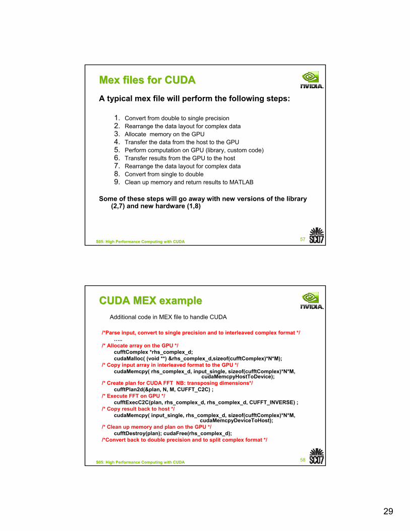
MexMex files for CUDAfiles for CUDAA typical mex file will perform the following steps:
1. Convert from double to single precision2. Rearrange the data layout for complex data3. Allocate memory on the GPU4. Transfer the data from the host to the GPU5. Perform computation on GPU (library, custom code)6. Transfer results from the GPU to the host7. Rearrange the data layout for complex data8. Convert from single to double9. Clean up memory and return results to MATLAB
Some of these steps will go away with new versions of the library (2,7) and new hardware (1,8)
58S05: High Performance Computing with CUDA
CUDA MEX exampleCUDA MEX example
/*Parse input, convert to single precision and to interleaved complex format */…..
/* Allocate array on the GPU */cufftComplex *rhs_complex_d;cudaMalloc( (void **) &rhs_complex_d,sizeof(cufftComplex)*N*M);
/* Copy input array in interleaved format to the GPU */cudaMemcpy( rhs_complex_d, input_single, sizeof(cufftComplex)*N*M,
cudaMemcpyHostToDevice);/* Create plan for CUDA FFT NB: transposing dimensions*/
cufftPlan2d(&plan, N, M, CUFFT_C2C) ;/* Execute FFT on GPU */
cufftExecC2C(plan, rhs_complex_d, rhs_complex_d, CUFFT_INVERSE) ;/* Copy result back to host */
cudaMemcpy( input_single, rhs_complex_d, sizeof(cufftComplex)*N*M, cudaMemcpyDeviceToHost);
/* Clean up memory and plan on the GPU */cufftDestroy(plan); cudaFree(rhs_complex_d);
/*Convert back to double precision and to split complex format */….
Additional code in MEX file to handle CUDA
30
59S05: High Performance Computing with CUDA
Initial studyInitial study
Focus on 2D FFTs.
FFT-based methods are often used in single precision ( for example in image processing )
Mex files to overload MATLAB functions, no modification between the original MATLAB code and the accelerated one.
Application selected for this study:solution of the Euler equations in vorticity form using a pseudo-spectral method.
60S05: High Performance Computing with CUDA
Implementation details:Implementation details:
Case A) FFT2.mex and IFFT2.mex
Mex file in C with CUDA FFT functions.
Standard mex script could be used.
Overall effort: few hours
Case B) Szeta.mex: Vorticity source term written in CUDA
Mex file in CUDA with calls to CUDA FFT functions.
Small modifications necessary to handle files with a .cu suffix
Overall effort: ½ hour (starting from working mex file for 2D FFT)
31
61S05: High Performance Computing with CUDA
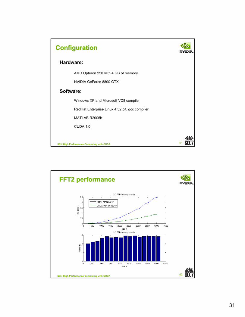
ConfigurationConfiguration
Hardware:
AMD Opteron 250 with 4 GB of memory
NVIDIA GeForce 8800 GTX
Software:
Windows XP and Microsoft VC8 compiler
RedHat Enterprise Linux 4 32 bit, gcc compiler
MATLAB R2006b
CUDA 1.0
62S05: High Performance Computing with CUDA
FFT2 performanceFFT2 performance
32
63S05: High Performance Computing with CUDA
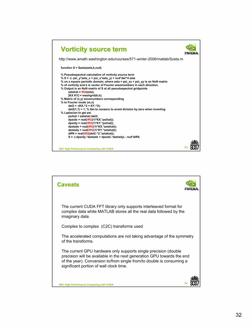
VorticityVorticity source termsource term
function S = Szeta(zeta,k,nu4)
% Pseudospectral calculation of vorticity source term % S = -(- psi_y*zeta_x + psi_x*zeta_y) + nu4*del^4 zeta % on a square periodic domain, where zeta = psi_xx + psi_yy is an NxN matrix % of vorticity and k is vector of Fourier wavenumbers in each direction. % Output is an NxN matrix of S at all pseudospectral gridpoints
zetahat = fft2(zeta); [KX KY] = meshgrid(k,k);
% Matrix of (x,y) wavenumbers corresponding % to Fourier mode (m,n)
del2 = -(KX.^2 + KY.^2); del2(1,1) = 1; % Set to nonzero to avoid division by zero when inverting
% Laplacian to get psi psihat = zetahat./del2; dpsidx = real(ifft2(1i*KX.*psihat)); dpsidy = real(ifft2(1i*KY.*psihat)); dzetadx = real(ifft2(1i*KX.*zetahat)); dzetady = real(ifft2(1i*KY.*zetahat)); diff4 = real(ifft2(del2.^2.*zetahat)); S = -(-dpsidy.*dzetadx + dpsidx.*dzetady) - nu4*diff4;
http://www.amath.washington.edu/courses/571-winter-2006/matlab/Szeta.m
64S05: High Performance Computing with CUDA
CaveatsCaveats
The current CUDA FFT library only supports interleaved format for complex data while MATLAB stores all the real data followed by the imaginary data.
Complex to complex (C2C) transforms used
The accelerated computations are not taking advantage of the symmetry of the transforms.
The current GPU hardware only supports single precision (double precision will be available in the next generation GPU towards the end of the year). Conversion to/from single from/to double is consuming a significant portion of wall clock time.
33
65S05: High Performance Computing with CUDA
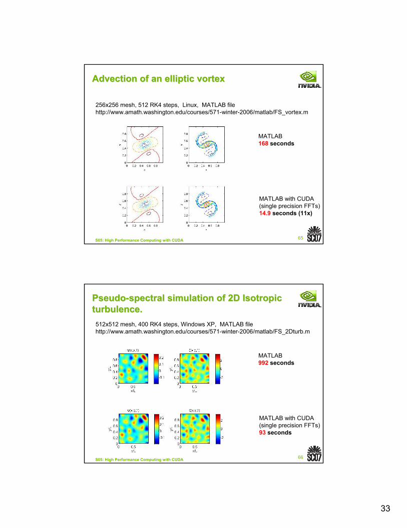
Advection of an elliptic vortexAdvection of an elliptic vortex
MATLAB 168 seconds
MATLAB with CUDA(single precision FFTs)14.9 seconds (11x)
256x256 mesh, 512 RK4 steps, Linux, MATLAB filehttp://www.amath.washington.edu/courses/571-winter-2006/matlab/FS_vortex.m
66S05: High Performance Computing with CUDA
PseudoPseudo--spectral simulation of 2D Isotropic spectral simulation of 2D Isotropic turbulence.turbulence.
MATLAB 992 seconds
MATLAB with CUDA(single precision FFTs)93 seconds
512x512 mesh, 400 RK4 steps, Windows XP, MATLAB filehttp://www.amath.washington.edu/courses/571-winter-2006/matlab/FS_2Dturb.m
34
67S05: High Performance Computing with CUDA
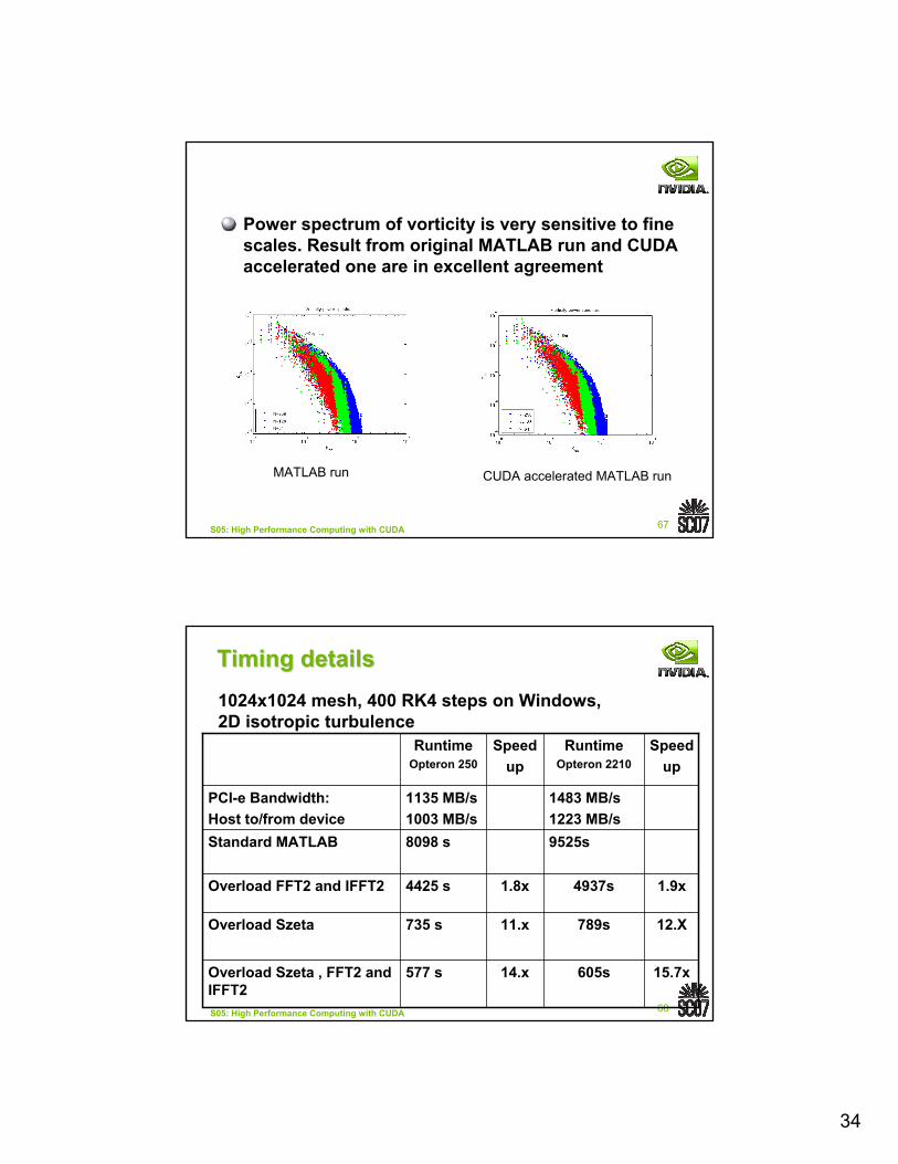
Power spectrum of vorticity is very sensitive to fine scales. Result from original MATLAB run and CUDA accelerated one are in excellent agreement
MATLAB run CUDA accelerated MATLAB run
68S05: High Performance Computing with CUDA
Timing detailsTiming details
1483 MB/s1223 MB/s
1135 MB/s1003 MB/s
PCI-e Bandwidth:Host to/from device
14.x
11.x
1.8x
Speedup
605s
789s
4937s
9525s
RuntimeOpteron 2210
Speedup
RuntimeOpteron 250
577 s
735 s
4425 s
8098 s
12.XOverload Szeta
Standard MATLAB
15.7xOverload Szeta , FFT2 and IFFT2
1.9xOverload FFT2 and IFFT2
1024x1024 mesh, 400 RK4 steps on Windows, 2D isotropic turbulence
35
69S05: High Performance Computing with CUDA
ConclusionConclusion
Integration of CUDA is straightforward as a MEX plug-inNo need for users to leave MATLAB to run big simulations:
high productivityRelevant speed-ups even for small size gridsPlenty of opportunities for further optimizations


![SC07 Optimization Harris.ppt [Read-Only] - GPGPUgpgpu.org/static/sc2007/SC07_CUDA_5_Optimization_Harris.pdf3 S05: High Performance Computing with CUDA Outline General optimization](https://static.fdocuments.us/doc/165x107/5ae0d5aa7f8b9ab4688ddbd2/sc07-optimization-read-only-gpgpugpgpuorgstaticsc2007sc07cuda5optimizationharrispdf3.jpg)