Univers

ity of

Cap

e Tow

n

SAVINGS, INVESTMENT AND ECONOMIC GROWTH IN NAMIBIA

A DISSERTATION SUBMITTED IN PARTIAL FULFILMENT

OF THE REQUIREMENTS FOR THE DEGREE OF

MASTER OF COMMERCE IN DEVELOPMENT FINANCE

OF

THE DEVELOPMENT FINANCE CENTRE (DEFIC)

GRADUATE SCHOOL OF BUSINESS

UNIVERSITY OF CAPE TOWN

BY

JULIUS NYERERE, NAMOLOH

NMLJUL002

DECEMBER 2017

SUPERVISOR: DR, AILIE, CHARTERIS

Univers

ity of

Cap

e Tow

n

The copyright of this thesis vests in the author. No quotation from it or information derived from it is to be published without full acknowledgement of the source. The thesis is to be used for private study or non-commercial research purposes only.

Published by the University of Cape Town (UCT) in terms of the non-exclusive license granted to UCT by the author.

i

PLAGIARISM DECLARATION

Declaration

1. I know that plagiarism is wrong. Plagiarism is to use another’s work and pretend that it

is one’s own.

2. I have used the American Psychological Association convention for citation and

referencing. Each contribution to, and quotation in, this thesis from the work(s) of other

people has been attributed, and has been cited and referenced.

3. This thesis is my own work.

4. I have not allowed, and will not allow, anyone to copy my work with the intention of

passing it off as his or her own work.

5. I acknowledge that copying someone else’s assignment or essay, or part of it, is wrong,

and declare that this is my own work.

Signature ______________________________

Student Name Surname: Julius Nyerere Namoloh

ii

ABSTRACT

This study examined the interaction between saving, investment and economic growth in

Namibia. The relationship between these variables is central to Namibia’s guiding

macroeconomic framework. However, empirical evidence has shown that the relationship

between saving, investment and economic growth depends on the country context. This makes

it important to understand the policy implications of the interaction between these variables in

Namibia. The specific objectives of the study were to investigate the causal relationship

between saving and investment and the impact of the saving-investment relationship on

economic growth in Namibia. The diagnostic testing using the Johansen cointegration test

revealed a long-run relationship between the study variables with one cointegrating equation.

The long run analysis was followed by Granger causality tests to understand short-run causal

relationships between the variables. Impulse response functions and variance decompositions

were also estimated to examine the interaction between the variables. The results from the

Vector Error Correction Model showed that there was a positive long-run relationship between

economic growth and investment, & savings and investment in Namibia. The Granger causality

test revealed a causal relationship between saving and investment, consistent with the long-run

analysis. The study implications are that a pro-saving policy can achieve increased investment.

However, the long run relationship between investment and economic growth implies that

investment should be made on a longer term for it to impact on economic growth. It is therefore

recommended that Namibia implements policies to encourage long term investments. This can

be achieved through waiving duty on capital goods and offering tax incentives to investors in

strategic sectors of the economy.

iii

TABLE OF CONTENTS

PLAGIARISM DECLARATION ............................................................................................... i

ABSTRACT ............................................................................................................................... ii

TABLE OF CONTENTS .......................................................................................................... iii

LIST OF FIGURES .................................................................................................................... v

LIST OF TABLES ..................................................................................................................... v

LIST OF ACRONYMS ............................................................................................................. vi

ACKNOWLEDGEMENT ....................................................................................................... vii

1.INTRODUCTION ................................................................................................................... 1

1.1 Background of the Research ............................................................................................. 1

1.2 Problem Statement ............................................................................................................ 4

1.3 Purpose and Significance of the Research ........................................................................ 5

1.4 Research Questions and Scope ......................................................................................... 6

1.5 Objectives of the Study..................................................................................................... 6

1.6 Layout of the Study .......................................................................................................... 6

2. LITERATURE REVIEW ....................................................................................................... 7

2.1 Introduction ...................................................................................................................... 7

2.2 Theoretical Review ........................................................................................................... 7

2.2.1 Determinants of Saving .............................................................................................. 7

2.2.2 Determinants of Investment ....................................................................................... 9

2.2.3 Impact of Saving and Investment on Economic Growth ......................................... 13

2.2.4 Public Investment Spending and Economic Growth ............................................... 13

2.3 Empirical Literature ........................................................................................................ 16

2.3.1 Empirical Studies on Saving and Investment .......................................................... 16

2.3.2 Public Investment and Private Investment ............................................................... 18

2.3.3 Empirical Evidence on the Relationship between Investment and Economic Growth

........................................................................................................................................... 18

2.4 Conclusion ...................................................................................................................... 21

3. RESEARCH METHODOLOGY ......................................................................................... 23

3.1 Introduction .................................................................................................................... 23

3.2 Research Approach and Strategy .................................................................................... 23

3.3 Econometric Model ........................................................................................................ 23

3.3.1 GDP .......................................................................................................................... 23

3.3.2 GDS .......................................................................................................................... 24

iv

3.3.3 Gross Capital Formation .......................................................................................... 24

3.3.4 Real Interest Rate ..................................................................................................... 24

3.4 Data Analysis Methods ................................................................................................... 25

3.4.1 Tests for Stationarity ................................................................................................ 25

3.4.2 Optimal Lag Length Selection ................................................................................. 25

3.4.3 Tests for Cointegration ............................................................................................ 26

3.4.4 Model Specification ................................................................................................. 28

3.4.5 Granger Causality Test ............................................................................................ 28

3.4.6 Impulse Response Functions.................................................................................... 29

3.4.7 Variance Decomposition .......................................................................................... 30

3.4 Conclusion ...................................................................................................................... 30

4. RESEARCH FINDINGS, ANALYSIS AND DISCUSSION ............................................. 31

4.1 Introduction .................................................................................................................... 31

4.2 Graphical Analysis ......................................................................................................... 31

4.3 Unit Root Tests ............................................................................................................... 33

4.4 Lag Length Selection ...................................................................................................... 36

4.5 Cointegration Tests ......................................................................................................... 36

4.6 Econometric Model ........................................................................................................ 38

4.6.1 Long Run Analysis .................................................................................................. 38

4.6.2 Short Run Analysis .................................................................................................. 38

4.6.3 Granger Causality Tests ........................................................................................... 39

4.6.4 Impulse Response Functions.................................................................................... 40

4.6.5 Variance Decomposition .......................................................................................... 44

4.7 Discussion of Results...................................................................................................... 46

4.8 Conclusion ...................................................................................................................... 47

5. RESEARCH CONCLUSIONS ............................................................................................ 48

5.1 Conclusions .................................................................................................................... 48

5.2 Recommendations .......................................................................................................... 49

5.3 Recommendations for future research ............................................................................ 49

References ................................................................................................................................ 51

APPENDIX 1: VECM Model .................................................................................................. 60

v

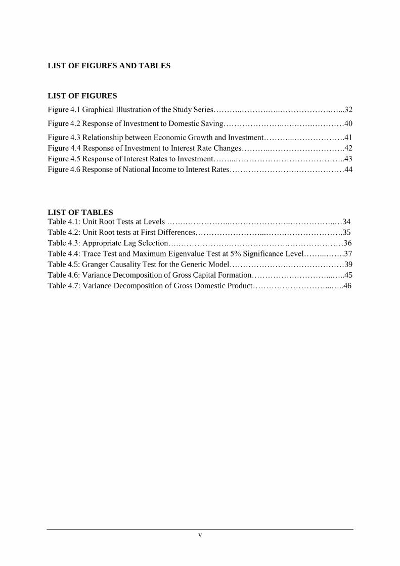
LIST OF FIGURES AND TABLES

LIST OF FIGURES

Figure 4.1 Graphical Illustration of the Study Series………..……….…..……………….…...32

Figure 4.2 Response of Investment to Domestic Saving…………………..….…….…………40

Figure 4.3 Relationship between Economic Growth and Investment………...……………….41

Figure 4.4 Response of Investment to Interest Rate Changes………..……………………….42

Figure 4.5 Response of Interest Rates to Investment……...…………………………………..43

Figure 4.6 Response of National Income to Interest Rates…………………….………………44

LIST OF TABLES

Table 4.1: Unit Root Tests at Levels …….……………..…………………..……………..…34

Table 4.2: Unit Root tests at First Differences……………………...…….………………….35

Table 4.3: Appropriate Lag Selection….……………….………………….…………………36

Table 4.4: Trace Test and Maximum Eigenvalue Test at 5% Significance Level……...…….37

Table 4.5: Granger Causality Test for the Generic Model………………….…………………39

Table 4.6: Variance Decomposition of Gross Capital Formation…………….…………...…..45

Table 4.7: Variance Decomposition of Gross Domestic Product………………………...…..46

vi

LIST OF ACRONYMS

GDP Gross Domestic Product

GCF Gross Capital Formation

GDS Gross Domestic Saving

NSA Namibia Statistics Agency

OECD Organisation for Economic Cooperation and Development

RR Real Interest Rate

TIPEEG Targeted Intervention Programme for Employment and Economic Growth

VAR Vector Autoregression

VECM Vector Error Correction Model

vii

ACKNOWLEDGEMENT

My special appreciation goes to my research supervisor, Dr. Ailie Charteris, she has been very

helpful and supportive and hands on during my research. Her professional guidance and her

knowledge in the field of research has directed and encouraged me to complete my research.

Special gratitude goes to my family, especially my dear wife and our children for

understanding, and affording me time and space during my research.

I am very grateful to the National Youth Council of Namibia for the financial support towards

my study.

Above all my thanks goes to my heavenly Father, the creator and giver of life and all blessings

of all kinds and in all forms. Thank you Lord for the wisdom!

1

1. INTRODUCTION

1.1 Background of the Research

Since 1990, Namibia’s economy has been characterised by low economic growth, high income

inequality and unemployment (National Development Plan 4, 2012). Given these challenges,

the government implemented the National Development Plan (NDP) as a guiding framework

to achieve its macroeconomic objectives of high and sustained economic growth, lower income

inequality and employment creation. However, economic growth remains below the desired

level of 5% for the country to achieve its growth targets by 2030 (NDP4, 2012). According to

the Organization for Economic Cooperation and Development (OECD) (2012) prior to 2012,

economic growth averaged around 3.3%. Although economic growth increased to 3.8% in

2011, it has decreased to 1.2% in 2016 (Word Bank, 2017). The statistics show that economic

growth has continued to deteriorate despite the government’s continued expansionary fiscal

policies which have widened the government deficit (OECD, 2016). The Namibian

macroeconomic framework is built on enhancing investment as the key to unlocking economic

growth. The NDP4 (2012) highlights that mobilising domestic savings and creating a conducive

environment for foreign direct investment are critical in increasing the investment levels in the

economy.

To understand the interaction between saving, investment and economic growth, it is important

to understand what constitutes the three variables and the underlying relationships between the

three series. Parkin (2012) defines saving as the amount of income that is not spent in paying

taxes or on the consumption of goods and services. He highlights that saving in the economy

can be split into two categories - private and public. Private savings consists of income

remaining after households and firms pay for expenditures in the current period, while public

saving is the tax revenue that is left unspent after the government implements its fiscal

initiatives.

These two forms of saving play a critical role in the achievement and maintenance of

sustainable growth and development. This is particularly so for developing countries like

Namibia, where domestic borrowing finances public sector expenditures. This is because

external capital flows to the private sector continue to decline (Uanguta, Haiyambo, Kadhikwa,

& Chimana, 2017). In 2017, Namibia’s long-term senior unsecured bond rating was

downgraded to junk status which will make it more expensive and difficult to access capital

2

from international credit markets. As such, further development initiatives may need to be

financed from domestic savings.

Gross Domestic Saving (GDS) in Namibia mainly comprises private savings (Mwinga, 2012).

This is because the government has maintained a consistent expansionary fiscal policy over

time leading to a widening of the budget deficit (Mwinga, 2012). Households and firms in

Namibia usually keep proceeds from economic activities at depository institutions. When

depository institutions invest these proceeds in the domestic market, they produce a multiplier

effect which results in the increase in national income. The Bank of Namibia (BON)’s (2004)

occasional paper postulates that the effects of saving and investment on economic growth are

two-fold: Firstly, demand for investment goods forms part of aggregate demand in the

economy. Thus, a rise in investment demand will stimulate production of investment goods

which in turn leads to high economic growth and development. Secondly, capital formation

improves the productive capacity of the economy in a way that the economy can produce more

output. Patrick (2017) highlights that GDS has fluctuated significantly over the past decade;

from 2003 to 2006, it increased from 10.28% of GDP to 26.17% after which it followed a

downward trajectory due to the global recession of 2007 and 2008. The latter has serious

implications for Namibia’s GDP where the growth rates have been consistently below the

targeted levels. The Namibian government needs to implement policies aimed at encouraging

national saving and ensure that this saving is invested into the domestic economy to enhance

economic growth.

Uanguta and Shimi (2015) concur that Namibia has seen a reduction in private savings over the

past decade while borrowing by individuals and firms has increased. This has resulted in an

increase in the ratio of household debt to disposable income. In 2014, household debt was a

staggering 86% of disposable income and this increased to 90% of disposable income in 2015.

However, the increase in household debt can also be a result of people taking credit for

investment purposes, as evidenced by the consistent growth of the property market over the

past decade. Similarly, these statistics can be an indication that firms are borrowing more to

expand their existing businesses. The use of credit to finance domestic investment can create

employment opportunities which result in economic growth since some growth theories

postulate that economic growth is a function of capital and labour (Stigliz & Walsh, 2006).

Technological progress from firms investing in better technologies can significantly improve

labour productivity and consequently economic growth. It is therefore important to critically

3

analyse the interaction between macroeconomic fundamentals to inform policies which results

in the optimal growth outcomes.

According to the neoclassical economic model, household saving is used to finance investment

(Solow, 1956). This implies that capital accumulation is best enhanced through the

implementation of policies that encourage household saving and capital flows from foreign

markets. The neoclassical reasoning implies that, capital flows from rich countries to poor

countries because of the higher returns provided in poorer countries. However, empirical

studies have questioned this relationship. Flassbeck (2012) argues that in a complex economy,

investment and saving decisions are made independently and hence a higher saving rate may

result in a fall in investment. The mobility of capital also contributes to the fact that despite

high domestic saving, investment rates may be low. Nikoforos (2015) further suggests that the

household saving rates for households at the bottom of the pyramid vary over time and adjust

endogenously to maintain a level of economic growth. He added that an increase in income

inequality or government deficit in an economy results in a decrease in the saving rate.

Given the above argument, growing inequalities and excessive expenditures have characterized

the Namibian economy for the past decade. The interaction between saving and investment is

hence, very important at this juncture, given that a significantly large proportion of the

population lives below the poverty datum line (NSA, 2012). The NSA reports that the poverty

incidence level in Namibia is 30%. Parking (2012) highlights that the major determinant of

saving is disposable income. Disposable income is defined as the portion of income that is left

after tax has been deducted. If disposable income is high, people tend to save more. Policies

aimed at encouraging saving across the population may not be effective since the majority of

Namibians have relatively low levels of disposable income. From the Keynesian theory,

consumers face liquidity constraints, thus it is difficult for them to interact with longer term

saving products when their income is not enough to cover for their day to day needs.

Another important factor that determines saving in Namibia is inflation. Uanguta and Shimi

(2015) highlight that the continuous erosion of household income by inflation reduces the

purchasing power of the Namibian dollar and the incentive to save. A high inflation rate also

reduces the return to saving because a dollar in the future will be worth less than a dollar today,

even when the discount rate is zero. The ability of Namibia to mobilise savings for investment

purposes is questionable given the income dynamics. For a developing country like Namibia to

4

finance the required investment, the economy needs to create adequate financial resources

through saving to fuel economic development. If local saving is insufficient, the country has to

rely on borrowing from external sources. However, borrowing from abroad may have adverse

effects on the country’s balance of payments in the long run.

Uangata and Shiimi (2015) point out that this increase in government expenditure in Namibia,

is largely financed through borrowing from both domestic and international debt markets, hence

the fiscal stance might have negative effects on the economy if maintained. Financing a deficit

through external debt diverts public resources to loan repayments and debt service. This reduces

public investment in areas that are relevant to private sector development such as infrastructure

(Greene and Villanueva, 1991). The current deficit of 6% of GDP is higher than Sub-Saharan

Africa’s average deficit of 4% (World Bank, 2017. These statistics show that the fiscal stance

in Namibia has been widely expansionary but the dividends in terms of growth have been low.

Namibia’s economic growth rate is too low to achieve the macroeconomic objectives set in the

vision 2030. Theory suggests that investment should spur economic growth. Investment is

expected to be higher when saving is high. However, empirical evidence shows that this

relationship does not hold all the time. The aim of this study is to determine the relationship of

these variables in Namibia and the policy implications of the relationships.

1.2 Problem Statement

Since independence, Namibia has struggled with low levels of economic growth, high levels of

inequality and unemployment. The guiding macroeconomic framework, the NDP4, has focused

on these three areas as a means to improve the welfare of Namibians. However, current statistics

show that Namibia’s growth rates have been consistently below targeted levels hence the

country is likely to miss the growth targets outlined in the vision 2030. The country has been

exploring ways to stimulate domestic saving to enhance investment and economic growth. The

relationship between saving, investment and economic growth in Namibia is not well

understood; thus, there is a need to investigate whether a pro-saving policy is an effective cure

for stunted growth as suggested by government policy.

Harbaugh (2004) highlights that when investment demand is high and capital flows are

constrained, the returns to saving are usually high; hence saving and investment are positively

correlated. He explained that the return to capital in most developing economies is usually high

5

because of scarce capital. However, contrasting evidence from Kaykci (2012) shows that there

are possibilities of short run divergence in the saving and investment relationship when there is

capital mobility. Due to the conflicting empirical evidence, understanding the relationship

between saving and investment is key in implementing appropriate policies to achieve

macroeconomic objectives.

Most developing economies focus on massive investment in infrastructure in pursuit of

economic progress. The NDP4 (2012) outlines that the government aims to stimulate income

growth through public investment programmes such as the Targeted Intervention for

Employment and Economic growth (TIPEEG). This programme was implemented between

2011 and 2014. Central to this programme was a massive investment in the provision of public

infrastructure. The National Planning Commission reported that the implementation of TIPEEG

would resolve the challenges the nation was facing in terms of unemployment and low

economic growth. Despite the implementation of TIPEEG, unemployment and low levels of

economic growth are still major challenges in Namibia, hence this brings into doubt the linkages

between investment and economic growth. Mwinga (2012) analysed secondary data from

Namibia’s Labour Force Surveys (NLFS for 1997, 2000, 2004 and 2008) and the 1993/94 &

2003/04 National Housing Income & Expenditure Surveys (NHIES), the results showed that

investment in public infrastructure had not been able to deliver outcomes in terms of economic

growth and improved welfare.

1.3 Purpose and Significance of the Research

International empirical studies on the relationship between saving, investment and economic

growth have produced varied results, suggesting that the relationship between the three

variables largely depends on the country context. Overall, there is a perception that high saving

leads to increased investment and ultimately economic growth. Namibia has also formulated its

guiding macroeconomic objectives based on this underlying relationship. However, there is a

dearth of research in this area in Namibia, with only a few briefing papers on the historical

trends of saving and investment rather than an econometric investigation of the relationship

between saving, investment and economic growth. As such, it is critical to ascertain whether

the government is indeed embarking on the correct path to achieve economic growth. This study

will thus provide answers to policy questions on the effectiveness of mobilizing domestic

saving to enhance investment and economic growth.

6

1.4 Research Questions and Scope

This study will attempt to answer the following questions:

Is there a causal relationship between saving and investment in Namibia?

What is the impact of saving and investment on economic growth in Namibia?

1.5 Objectives of the Study

The objectives of the study will be to:

investigate whether there is a causal relationship between saving and investment in

Namibia and

to determine the impact of saving and investment on economic growth in Namibia.

1.6 Layout of the Study

This study consists of five chapters. Chapter one provided the background to the study and

elaborated on the problem statement. This chapter also presented the research questions and the

guiding objectives of this study. Chapter two contains the literature review including both the

theoretical framework of the relationship between saving and investment and economic growth

as well as the results of empirical studies that have investigated the determinants of these

variables and their relationship in various countries. The methodology employed in this study

to answer the research questions is described in chapter three, and chapter four presents the

findings from the empirical analysis. The conclusion of the study is presented in chapter five,

along with recommendations from the findings of the study.

7

2. LITERATURE REVIEW

2.1 Introduction

This chapter reviews the literature relevant to this study, including the theoretical framework

and empirical studies on the determinants of saving and investment, the relationship between

saving and investment and the link to economic growth. The relationship between public and

private investment is also discussed as this relationship has strong implications for growth.

2.2 Theoretical Review

2.2.1 Determinants of Saving

As previously defined, saving is the amount of income that is not spent in paying taxes or on

the consumption of goods and services. The determinants of saving can thus be understood

from the determinants of consumption. Keynes argued that saving is an increasing function of

income (Keynes, 1936). The Keynesian consumption function has two components - an

autonomous component, which is the minimum consumption level an individual consumes that

is independent of their economic status, and a component that increases marginally as income

increases.

Following the Keynesian approach to consumption, Duesenberry (1949) argued that the

relationship between consumption and income is not as simple as Keynes had postulated.

Duesenberry (1949) argued that consumption depends on an individual’s percentile position in

an income distribution. The second hypothesis is that consumption is not merely a function of

absolute income but is affected by relative income measures attained in the past. The

implication of this theory is that consumption does not decrease as income decreases.

According to Duesenberry (1949), the utility obtained from any given consumption level

depends on the magnitude of the level of consumption relative to what the rest of the society is

consuming rather than the absolute consumption level. As such Duesenberry (1949) argued that

the saving rate does not increase proportionately with the rate of income growth but rather that

the propensity to save increases proportionately with increases in an individual’s percentile

position in the income distribution.

Friedman (1957) departs from both Keynes and Duesenberry’s approach to consumption. In his

theory of permanent income, he proposes that saving does not depend on long-term current

income but permanent income. He argues that short-term windfalls or capital gains do not

influence the consumption decisions of individuals as they wish to smooth consumption over

8

their lifetime. Instead temporary windfalls will affect an individual’s saving behavior

(Friedman, 1957). In his theory, he attempts to explain how consumption smoothing is the main

motivation of individuals spreading their incomes almost uniformly over their life cycle. He

stated that a person’s current consumption is affected by changes in permanent income rather

than temporary changes in income. He highlights that people spread out transitory changes in

income over time to derive uniform consumption. This theory departs from the traditional

Keynesian marginal propensity to consume approach to consumer behaviour.

An extension of the permanent income hypothesis is the life cycle hypothesis which assumes

that the objective of saving is to smooth consumption levels over an individual’s lifetime. Ando

and Modigliani (1963), in their ‘life cycle hypothesis of saving’, consider that economic agents

save money depending on the stage of the life cycle they are in. That is, they borrow when they

are young, save during working years and spend during retirement. Kohl and O’Brien (1998)

highlighted that the life cycle model assumes that an individual’s utility depends solely on their

given level of consumption and their time horizons. The extended life cycle model postulates

that the primary effect of income on consumption is offset by secondary factors such as induced

labour supply. This argument is based on the assumption that labour supply changes in response

to income and other substitutes such as leisure. When the income effect dominates, individuals

will increase their supply for labour and retire early. This results in them saving more to cater

for longer retirement periods. When the income effect is low, individuals consume more leisure

and supply less labour. This results in lower saving levels as individuals anticipate longer

working periods (Kohl & O’Brien, 1998).

Income, however, is not the only contributing factor to saving within a country. Interest rates,

economic expectations and government taxes are among the factors that have an impact on

saving decisions. From the liquidity preference theory of Keynes (1936), the quantity of money

people desire to hold is inversely proportional to the prevailing interest rates. Keynes argues

that when interest rates are high, people prefer to hold their wealth in interest-bearing assets.

Higher interest rates induce people to save more since interest rates are the opportunity cost of

holding money. This is also similar to the Mackinon and Shaw hypothesis which argues against

interest rate ceilings after establishing a positive relationship between interest rates and saving.

However, some counter arguments on the relationship between saving and interest rates have

been proposed in the literature. For example, Schmidt-Hebbel and Serv´en (1999) argued that

due to behavioral factors such as hyperbolic discounting and loss aversion, the relationship

9

between saving and interest rates becomes very weak. Keynes, in his liquidity preference

theory, also documented that high interest rates may not result in high saving levels because

economic agents face liquidity constraints resulting in a tradeoff between short-term

gratification and long-term goals.

Economic expectations also play a major role in influencing consumption and saving decisions.

One of the main reasons for saving is the precautionary motive. Households save in anticipation

of uncertain and difficult times where there is a risk of decreasing income. These uncertainties

may come from macroeconomic instability and inflation, exchange rate volatility or the

financial system. Inflation anticipation by economic agents may lead them to discourage saving

because inflation reduces the purchasing power of the amounts they hold in savings (Fischer,

1993).

The size of the fiscal deficit or surplus is another factor that could affect national saving. A low

fiscal deficit or surplus promotes public saving and hence national saving. This effect is greater

in developing countries with subsistence consumption and liquidity constraints (Corbo and

Schmidt-Hebbel, 1991). The level of taxes and government spending can also influence saving

(Blanchard & Johnson, 2013). Increased government spending is usually followed by an

increase in taxes or government borrowing. The increase in taxes lowers the disposable income

in the economy thus economic agents will save less, according to Keynesian theory. However,

Barro (1974) presents an alternative theory, the Ricardian equivalence theory, that increasing

public deficits leads to an anticipation of future tax increases by economic agents, leading to an

increase of saving.

2.2.2 Determinants of Investment

Early theories of investment, were based on the work of Clark (1917) in what was referred to

as the accelerator theory. The accelerator theory is based on the basis that an increase in national

income leads to an increase in investment. Under this theory, an increase in national income

causes an increase in investment by a multiple amount. The larger increase in investment

spending from a smaller increase in national income is known as the multiplier process (Clark,

1917).

This was further developed by Jorgensen and Hall (1967) under the neoclassical school of

thought. The neoclassical school views the stock of capital (i.e. investment) as a positive

function of income (Bernomi, 1945). The neoclassical theory highlights that investment at

equilibrium is determined by price factors of production which is represented by the interest

10

rate (Schmidt-Hebbel, Corbo, Vittorio & Klaus, 1999). Neoclassical theory highlights that there

is a negative relationship between real interest rates and investment; high interest rates imply

that the cost of borrowing is high and thus the return on investment is eroded by the cost of

servicing debt (Benoni, 1945).

According to Kopcke (1985) the main distinguishing factor between the accelerator model and

the neoclassical model is that the neoclassical models moves away from the bivariate

specification of the investment function by including prices, interest rates and proxies of tax

laws. The neoclassical models postulate that factor prices especially the cost of capital should

be accounted for when explaining investment behavior.

Following the neoclassical school of thought, many governments used interest rate ceilings to

ensure that capital is affordable to investors. This resulted in interest rates being pegged at low

rates which were at times lower than the rate of inflation. This eroded the incentive to save and

the result was a lack of funds in the formal financial system. The result was a phenomenon

termed by MacKinnon and Shaw (1973) as financial repression. MacKinnon and Shaw (1973)

argued against the neoclassical reasoning which postulated that lower interest rates resulted in

higher levels of investment. According to MacKinnon and Shaw (1973), low interest rates in

economies result in capital shortages as money moves to countries where capital returns are

higher. McKinnon and Shaw (1973) argued that high interest rates, by encouraging saving,

increase the volume of available domestic credit, which increases investment. The McKinnon

and Shaw hypothesis highlights that it is not the cost of financial resources that hinder

investment, but rather the lack of available financial resources for investment. McKinnon and

Shaw (1973) suggest that financial development can foster investment and thus economic

growth through the reduction of credit constraints for investment. That is, low financial

development creates credit constraints which may negatively affect private investment. In

countries with poorly developed financial systems and equity markets, bank loans are the only

sources of credit available to people. Consistent with this view, in the traditional endogenous

growth models, Greenwood and Jovanovic (1990), Saint-Paul (1992) and Pagano (1993)

highlight the importance of increased financial intermediation through opening up the financial

sector to increase competition. Competition in the financial sector will result in lower costs of

borrowing therefore affording entrepreneurs greater access to credit to finance private

investment.

11

The institutional environment is widely recognized as a key factor that influences investment

especially in developing countries (Stigliz & Walsh, 2006). North and Thomas (1973) argue

that the fundamental explanation of the differences in paths of long-term growth lies in the

institutional differences between countries. It is the institutions, defined by North (1990) as the

set of rules in a society that allow greater appropriation of the gains from individual activity,

which determines investment, innovation and ultimately economic growth.

Another factor that has a strong impact on investment and that is closely linked to the

institutional environment is uncertainty and instability. Weak institutional structures lead to

lack of predictability of the macroeconomic environment and policy inconsistencies (Barro,

1974). The lack of continuity and stability in long-term economic policies leads to permanent

instability in the economic environment and hence to less incentives to invest. Instabilities and

uncertainties can also affect investment (Brue, McConnell, & Fynn, 2014). If investors expect

good economic conditions, then investment is likely to increase. If, however, they expect harsh

economic conditions, then investment may fall. Lack of institutional structures, instabilities and

uncertainties increase the risk of losing invested capital. In addition, the risk of war and the

absence of institutions protecting property rights discourage investment.

Risk is widely recognised as an important determinant of investment (Stiglitz & Walsh, 2006).

Investors usually want investments that will guarantee them of a profit. They only invest in

risky projects if the returns are high. Firms with lower credit ratings find it very difficult to

finance their investments through borrowing. The uncertainty and instability in the

macroeconomic environment described above can also be seen as a component of risk.

Another factor that impacts investment is government spending; however, it is unclear whether

the effect is positive or negative. Proponents of government spending, particularly the

Keynesian school of thought, argue that an increase in government spending leads to an increase

in investment spending. This increases the aggregate demand in an economy thus increasing

national income (Keynes, 1936). A common argument against persistent government spending

is the crowding-out phenomenon. According to Blanchard and Johnson (2013), crowding-out

occurs when government spending in the economy results in lower private investment in an

economy. The impact of spending intervention can be either at the supply or demand side.

Crowding-out occurs when government implements an expansionary fiscal policy by increasing

its spending or reducing taxes. The government has to finance the increase in expenditure

through borrowing and hence it will compete with the private sector for available funds in the

12

market. The increase in demand for loanable funds results in an increase in interest rates and

thus it becomes more expensive for the private sector to implement investment projects due to

the high cost of borrowing. Another form of crowding-out is resource crowding-out (Sloman,

Wride, & Garratt, 2015). This occurs when the government competes with the private sector

for labour and raw materials. If the economy is operating near full employment, resources used

by the government become unavailable to the private sector.

On the other hand, Crowding-in refers to the increase in private sector investment which is

caused by government activities. This arises from a reduction in government spending or an

increase in taxes which leads to the reduction in interest rates in the loanable funds market and

thus an increase in investments. This is so because a fall in interest rates makes it favourable

for borrowing which will in turn increase investment. Within the framework of restrictive fiscal

policy, a government can reduce its deficit by increasing taxes or reducing government

spending (Obrien, 2013)

The degree of trade openness is another important determinant of investment. This is typically

measured by trade flows (exports minus imports), which may have a positive effect on

investment (Levine and Renelt, 1992), as it can expand the opportunities for firms to achieve

greater economies of scale and efficiency in investment (Krueger, 1978). Trade liberalization

also allows ideas and technology transfers with the import of high value added products, which

promotes the adoption of these technologies and new working methods and standards in

domestic production (Edwards, 1992). However, openness to trade may, in certain situations,

adversely affect domestic investment. Indeed, poor countries would not have all the

prerequisites to withstand international competition with multinational companies from rich

countries. Openness could result in flooding these countries with imported products that

predominantly consist of consumer goods, while they have all the difficulties in exporting their

manufactured goods (Ndikumana, 2000). This can cause a collapse of their domestic sector.

The exchange rate may also affect the investment decisions of firms. In theory, there may be

two opposing effects. When the domestic currency depreciates, exports are likely to increase

because the goods become cheaper, which encourages investment due to greater demand. But

this effect may be offset by the rising cost of imported goods. The currency appreciation

produces the opposite effect (Campa and Goldberg, 1999).

13

2.2.3 The Impact of Saving and Investment on Economic Growth

The flagship Keynesian approach to economic progress is the Domar (1946) model which

assumes that aggregate demand grows at the same rate as national income (Gardner, 2005).

Investment is one of the components in the aggregate demand function and the investment-

output ratio is defined as the rate of capital accumulation. Domar (1946) explains that there is

a linear relationship between capital and output and economic growth is achieved when the

saving rate increases, increasing the level of productivity of capital or decreasing the

depreciation of capital stock. Commendatore, Panico and Pinto (2011) highlighted that the

fundamental Keynesian approach to growth is based on three distinguishing principles. Firstly,

the economy may not operate at full employment; secondly, saving and investment decisions

are independent of each other and as such, there is no causal link between saving and

investment; and thirdly, the presence of autonomous demand in the economy may affect the

rate of income growth.

The neoclassical school of thought on economic growth assumes that consumers always save a

fixed amount of income and allocate this towards investment. This school of thought gave

prominence to the Solow (1956) growth model which states that output is a function of labour

and the level of capital stock. The Solow model assumes that the level of capital stock depends

on the discounted levels of capital stock and investment in the previous year (Solow, 1956). An

increase in saving implies an increase in investment hence this results in national income

growth in the short-run. However, Solow (1956) argues that in the long-run, higher saving and

investment have no effect on economic growth. That is, in the long-run there is a tradeoff

between capital accumulation and capital depreciation. The result is that the economy maintains

equilibrium at a steady state when the rate of capital accumulation is equal to the depreciation

of capital, hence there is no contribution of investment to national income. The income at this

steady state is called the natural rate of income (Guo, Dall’erba, & Gallo, 2013).

2.2.4 Public Investment Spending and Economic Growth

The government stance on taxes has a significant impact on consumption levels and ultimately

saving (Barnheim, 1989). There are three theoretical explanations as to how taxation affects

consumption and saving (Manuel, 2004). The first is the neoclassical theory which postulates

that economic agents forecast future economic conditions and make decisions based on their

perception of the future. The link between government investment spending and economic

14

growth can be explained by the tax smoothing theory. This school of thought is known as the

Ricardian view which assumes that the government is a responsible social planner. The ultimate

objective of the government is to increase social welfare by maximizing the utility of the public.

The government achieves this by financing its initiatives through taxes. The welfare in the

economy improves through private consumption and leisure consumption.

The tax smoothing theory assumes that social welfare is improved when expenditure is

increased on leisure and private goods. However, the public will experience welfare losses

when investment spending on public goods increases. Spending on public goods is

characterized under defense spending. When the government increases its spending from

borrowing, the public anticipates higher future taxes hence will save more to finance higher

taxes in the future. Government expenditure under this model will have no effect on national

income since the public does not adjust their consumption behaviors in response to fiscal policy

initiatives. Under this view, the main motivation to save is consumption smoothing which

means individuals want to maintain their consumption levels over their lifetime. A tax policy

which results in tax cuts will result in no change in consumption but increase saving behavior

among individuals. This is because economic agents understand that a tax cut today simply

means that government must raise taxes in future to close the deficit resulting from the

expansionary fiscal policy. The implication is that fiscal policy in the form of reduced taxes

does not have an effect on consumption, aggregate demand and income in the economy.

The second school of thought is the model of opportunistic behavior. Under this model,

economic agents are myopic hence they overestimate the benefits from an expansionary fiscal

policy while underestimating the burden of increased taxes in the future (Manuel, 2004). He

added that under models of opportunistic behavior, expansionary fiscal policies can be used to

artificially alter economic progress during election periods to gather political support. Once a

government is elected, it will have to deal with servicing the debt and hence government

investment expenditure will have to be aligned to economic objectives.

Models of opportunistic behavior are consistent with the Ricardian view. Barnheim (1989)

explains that deficits merely shift the payment of taxes to future generations hence they leave

dynastic resources unaffected. Thus, deficit policy is a matter of indifference. This follows the

Keynesian view which assumes that individuals face liquidity constraints which result in a high

propensity to consume from their incomes. This assumption provides a distinct deviation from

neoclassical reasoning because temporary tax reduction in this case will cause an immediate

15

increase in consumption and ultimately aggregate demand. From the Keynesian theory,

government investment expenditure has been seen as a critical tool to achieve national growth.

The adoption of Keynesian reasoning led to most countries implementing expansionary policies

to stimulate aggregate demand. This resulted in increases in inflation levels without real change

in output (Friedman, 1956). This view was also supported by Mitchell (2005) who argued that

previous studies which concluded that persistent expansionary policies can be used to pursue

growth objectives were often characterized by methodological flaws in their analysis. Mitchell

(2005) highlighted that correcting for these errors would often show that government spending

does not stimulate economic growth. Mitchell (2005) juxtaposes the Keynesian view by

presenting an alternative argument that government can only implement expansionary fiscal

policies through withdrawing money from the economy through taxes. He highlighted that

often the government withdraws money from more productive sectors to channel it towards

unproductive social objectives. Mitchell (2005) argues that in the 1970s government investment

expenditure to stimulate economic growth was associated with economic stagnation while

higher growth in the 1980s was achieved by lowering taxes and reducing government

expenditure.

Similar to models of opportunistic behavior, Manuel (2004) proposes the third model which

seeks to explain the effect of taxes on consumption and investment, which he terms ideological

behavior. He argues that this model can be used to distinguish governments into two categories:

capitalist or socialist. A government’s approach to investment expenditure and economic

growth entails a tradeoff between efficiency and equity; predominantly capitalist governments

tend to channel investment towards the most productive sectors of the economy leading to

economic growth while socialist governments channel resources towards the greater good. The

main challenge is that capitalist governments tend to achieve economic growth without

economic development while socialist governments tend to achieve equality at the cost of

economic stagnation (Manuel, 2004).

Theory has produced divergent views on the role of the government in the economy. Proponents

of the classical school of thought often argue that government should not intervene in the

economy. This is based on the views of Smith (1977) who brought forward the concept of the

invisible hand in the market. Smith argues that markets can efficiently allocate resources on

their own to the most productive sectors and that government cannot use policy instruments to

maintain macroeconomic variables above their natural rate. This reasoning is challenged by

16

Keynes (1936) who argued that government must intervene in the economy to cure market

failures and pursue growth objectives.

2.3 Empirical Literature

Several studies have estimated the saving and investment function in developing countries,

particularly in sub-Saharan Africa (Schmidt-Hebbel, Corbo, Vittorio & Klaus, 1999). Many of

these studies have used national saving and investment figures while only a few have focused

on private saving and investment. However, it is of great importance to determine factors that

influence changes in private saving and investment, as these are the main components of

aggregate saving and investment in many countries. This is particularly true in Namibia where

aggregate saving consists of only private saving due to the fact that the government has

consistently maintained a budget deficit since independence. Further, policies that are geared

to raise the level of saving and investment generally focus on these two aggregates. Typically,

a number of macroeconomic variables have been included in the saving and investment models

to account for the effects of monetary, fiscal and exchange rate policies. The inclusion of

macroeconomic stability factors in the saving and investment models is done on recognition

that these factors have significant influences on saving and investment. This section provides

an overview of the empirical approaches used by researchers in trying to understand the

relationship between saving, investment and economic growth.

2.3.1 Empirical Studies on Saving and Investment

Studies on the investment and saving relationship have yielded different results even when

researchers used the same methodological approaches. Furthermore, the results vary even when

the study samples consider countries that are similar in terms of their development progress.

The genesis of the study of the saving-investment relationship in the empirical economics

literature is typically attributed to the seminal study by Feldstein and Horioka (1980). Following

their findings, the relationship between saving and investment has been the subject of intense

research over the past three decades. Feldstein and Horioka (1980) interrogated the question

about whether saving remains in the country of origination to finance domestic investment. In

addition, they analysed the optimal tax and saving rates by drawing in elements of capital

mobility. Using data for 21 OECD countries for the period 1960 to 1974, they found that nearly

all incremental saving remains in its country of origin. Incremental saving is the increase in

GDS from an increase in saving rate. The countries under consideration were industrialised

17

countries and the researchers point out that under perfect capital mobility, there should be no

relationship between domestic saving and private investment. The results of the study revealed

that the differences between private investment in the countries under study was proportionate

to the differences in saving rates between countries. This contrasts the view that capital should

flow to countries with the highest return. The study findings are consistent with the view that

portfolio preference and institutional rigidities often result in additional saving being channeled

towards domestic investment.

The implementation of capital liberalisation in Turkey in 1989 provided a strong basis for

testing the findings of Feldstein and Horioka (1980) that under capital mobility there would be

no relationship between saving and investment. For this purpose, Kaya (2010) used private

investment and national quarterly data on saving for the period 1984Q1 to 2007Q3. The

analytical technique used in this study was the Autoregressive Distributed Lag (ARDL) bounds

testing. The study found that there was a strong long-run relationship between national saving

and private investment. These results are inconsistent with Feldstein and Horioka’s (1980)

views that under capital liberalization there is no relationship between saving and investment.

However, this does not invalidate Feldstein and Horioka’s (1980) claim because even under a

liberalized capital market, investors may still prefer to hold domestic portfolios compared to

foreign ones resulting in a positive relationship between domestic saving and investment.

Dritsaki (2015) investigated the saving and investment relationship in Greece. He used data on

saving and investment rates from 1980 to 2012. The empirical analysis involved unit testing

using the Augmented Dickey Fuller (ADF) tests while cointegration tests were conducted using

ARDL bounds testing. The analysis revealed that there was a short- and long-run relationship

between saving and investment. The cointegration tests were complemented by Granger

causality tests which revealed that saving Granger-causes investment and this relationship is

unidirectional. Further to this, variance decompositions revealed that domestic saving is the

main determinant of investment in the long-run. This is consistent with the Keynesian theory

which assumes that investment is financed from investment thus an increase in saving implies

an increase in investment.

18

2.3.2 Public Investment and Private Investment

The relationship between public and private investment is also important to illustrate the

theoretical arguments explored in this study. A study conducted in Zimbabwe by Ndovorwi

(1997) investigated the impact of public policy on private capital formation. Ndovorwi (1997)

used annual data for the years 1980 to 1990, which is decomposed into quarterly observations

using interpolation. Private investment is regressed on public investment, bank credit to the

private sector, the inflation rate, output growth rate and lagged private investment. In the short

run, Ndovorwi (1997) revealed that public investment, whether infrastructural or non-

infrastructural, crowds out private investment. However, in the long-run Ndovorwi (1997)

concluded that public infrastructure investment is positively related to private investment.

Ndovorwi’s (1997) findings of a crowding in effect of public investment spending in the long-

run are broadly consistent with the findings of most studies. For example, a study in Turkey by

Chibber and Wijnbergen (1992) found that, with a three-year lag, an increase in the share of

infrastructure investment in public investment has a positive impact on private investment.

Furthermore, Mataya and Veeman (1996) analysed the investment behaviour in Malawi’s

private and public goods sectors between 1967 and 1988, considering partial liberalisation and

contractionary fiscal and monetary policies associated with the International Monetary Fund

supported Economic Structural Adjustment Programmes (ESAP). A Granger causality test was

employed to assess whether one- or two-way causality exists between private and public

investment. A two-way causality was found between the two types of investment. The effect of

private investment on public investment and vice versa was established as a positive

relationship. However, their results suggested that public investment is not influenced by

expected output. Contractionary fiscal and monetary policies had a negative effect on public

investment and a negative effect on private investment.

Another study by Pereira (2001) tested the effects of public investment on the evolution of

private investment in the United States using the Vector Autoregression (VAR) model and

impulse response functions. The empirical results showed that at the aggregate level public

investment crowds in private investment.

2.3.3 Empirical Evidence on the Relationship between Investment and Economic Growth

An important study which depicts the Namibian macroeconomic context by Manner (2014)

investigated whether infrastructure spending by governments, which is typical of developing

19

economies, can be used to accelerate economic growth. The study focused on big capital

investments by government and how these explained economic growth. Manner (2014) focused

on low income countries using data on expenditure and economic growth between 1992 and

2012. Panel regression analysis was conducted and the results revealed a weak positive

relationship between public investment spending and national income growth. The findings

showed that government spending in the previous year did not have a significant impact on

growth realized in the current year. The weak positive relationship between investment

spending and economic growth was only realized in the current year and was not sustained into

the future, suggesting that investments should result in improved long-term productivity in

order to improve a country’s growth prospects. Improvements in long-term productivity are

difficult to attain over a short period thus resulting in a weak link between investment and

economic growth. Manner (2014) explains that public investment expenditure in most

developing countries tends to be financed by borrowing and has often been ineffective in

improving economic growth because of incentive problems, poor investment analysis and

divergent personal and political interests. These findings are consistent with the results from

Ndovorwi (1997) and Perreira (2001) who showed that public investment crowds out private

investment resulting in a weak relationship between investment and economic growth.

Verma (2007) investigated the relationship between investment and economic growth in India

over the period 1950 to 2003 using the ARDL approach. The results showed that there is no

relationship between investment and economic growth in both the short and long-run which

contrasts with the commonly accepted growth models. In a similar study, Watson, Ilegbinosa

and Micheal (2015) explored the impact of domestic investment (both public and private) on

economic growth in Nigeria. The sample consisted of data from 1970 to 2013. The econometric

analysis included a multivariate regression and cointegration testing. The results showed firstly

that government investment had a crowding out effect on private investment and secondly that

public investment had no effect on economic growth.

It is worthwhile to note that some empirical studies show that investment has been a key driver

of economic progress. For example, Mehanna (2003) conducted a study on the causality

between investment and national income growth. He used a sample of 80 developing economies

over the period 1982 to 1997. The methodology used in this study was simultaneous equation

modelling based on the new growth model. The findings revealed a strong positive link between

investment and national income growth suggesting that investment predetermines economic

20

growth. Moreover, trade openness was not significant in explaining economic growth once

investment was included in the model. However, the results revealed that trade openness was a

significant predictor of investment and thus affected economic growth through the investment

channel.

Another study conducted in Arab states showed that in some countries, increases in investment

levels have been coupled with increases in levels of economic growth (Roudet, Lahreche &

Zaher, 2016). However, he notes that the relationship between national income growth and

investment is weakening over time. This is evidenced by the decrease in total factor

productivity’s contribution to economic growth. Wong (2012) also looked at the association

between economic growth and investment. He used panel regression using a sample of both

advanced and less advanced economies. In his approach, they adopted the neoclassical growth

theory as the framework which assumes a concave production function and positive returns to

capital but they exhibit diminishing returns as the ratio of capital to output rises. This

relationship implies as the level of capital increases, the effect of lagged investment on

economic growth decreases and could turn negative. Wong (2012) documented a negative

relationship between investment and economic growth in high income countries. This was

consistent with Getty (2010) who argued that despite the fact that the United States managed

to consistently increase its investment and saving rate, there was still no evidence to show that

this resulted in improved economic growth. However, in low income countries the results

showed a positive relationship between investment and economic growth consistent with

Keynesian theory.

Aghion, Comin and Howitt (2009) explored the question of whether a country can grow faster

by saving more from both a theoretical and empirical perspective. The theoretical model

postulated that economic growth is attained through innovation that enables local sectors to

advance so as to catch up with frontier technologies. Under this theoretical model, saving plays

an important role in financing innovation and consequently economic growth. The empirical

approach used a cross-country regression (including both advanced and developing economies)

on saving, investment and economic growth for the period 1992 to 2005. The study concluded

that national saving is positively associated with investment and economic growth in

developing economies but not in advanced economies.

21

A study focusing on the dynamic interaction between domestic investment, foreign direct

investment (FDI) and economic growth in Pakistan was conducted by Ullah, Shah and Khan

(2011) over the period 1976 to 2010. The econometric analysis included Johansen cointegration

test to examine the relationship between variables in both the short- and long-run. The Toda-

Yamamoto methodology was used to test for causal linkages between variables. The

econometric analysis revealed that there was a long-run relationship between domestic

investment, FDI and economic growth while the causality analysis revealed that FDI and

domestic investment have a two-way causal relationship.

Zafar (2011) investigated the relationship between domestic investment, export and economic

growth in Saudi Arabia. The study used data from 1970 to 2007. Cointegration analysis was

done to test for the existence of a long-run relationship between the study variables. The results

revealed that there was a long-run relationship between the three variables. The findings also

demonstrated that only domestic investment significantly contributed to economic growth in

both the long- and short-run.

A study by Tien (2016) in Vietnam looked at the relationship between FDI, domestic

investment and the exchange rate. The sample included data from 1985 to 2015. The Johansen

cointegration test was used to examine the long-run relationships of the variables while Granger

causality tests were undertaken and a VAR model estimated to investigate the interaction

between the variables in the short-run. The study showed that domestic investment and export

growth Granger caused FDI inflows and economic growth. The study revealed that FDI inflows

did not increase economic growth in Vietnam.

The above empirical evidence produces contrasting views on the relationship between

investment and economic growth. Studies conducted in low income countries tend to reveal a

weak relationship between investment and economic growth. Evidence from Arab countries

leans towards a positive relationship between investment and economic growth. The studies

that split investment into domestic and FDI show that domestic investment is the main driver

of economic growth compared to FDI.

2.4 Summary

In summary, the evidence learned from the past research and economic theories shows that the

link between saving, investment and economic growth is still elusive. The empirical analysis

showed that the link between saving and investment is strongly dependent on capital mobility

22

hence this relation differs across countries. The empirical literature review showed that in some

cases, public investment crowds out private investment thus reducing the impact on economic

growth. As such, this compromises the impact of investment on economic growth. In light of

this uncertainty, this study seeks to investigate the interaction between saving, investment and

economic growth in Namibia. The following chapter describes the research methodology used

to answer this question.

23

3. RESEARCH METHODOLOGY

3.1 Introduction

This section describes the methodology that was followed to answer the research questions. An

overview of the data sources, the model specification and justification for the choice of

variables is provided.

3.2 Research Approach and Strategy

To achieve the objectives of this empirical study, secondary data was collected from the

Namibian National Accounts published by the Word Bank for the twenty-four-year period

1992-2015. Annual data was collected on GDS, Gross Capital Formation (GCF), GDP and the

real interest rate (RR). Quarterly data would have been ideal given the time period but only

annual data was available for the study variables. The E-Views software package was used to

analyse the data because of its efficacy in examining time-series data.

3.3 Econometric Model

As indicated in chapter 2, all growth theories indicate that saving and investment play a critical

role in economic growth (Dritsaki, 2015). As indicated previously, the goal of this research was

to assess the impact of these two variables on economic growth in Namibia while also looking

at the direct interaction between saving and investment in the country. Alongside saving and

investment, the interest rate was also included as an explanatory variable following the

MacKinnon and Shaw (1973) hypothesis that interest rates tie saving and investment together,

as discussed in chapter 2. The equation which forms the basis of this analysis can thus be

expressed as follows:

𝐺𝐷𝑃𝑡 = 𝛼0 + 𝛼1𝐺𝐷𝑆𝑡 + 𝛼2𝐺𝐶𝐹𝑡 + 𝛼3𝑅𝑅𝑡 + 𝑒𝑡 (4.1)

The variables used to estimate these equations are described in detail below.

3.3.1 GDP

The OECD (2016) defines GDP as the monetary value of the final goods and services produced/

rendered in a country for a given time period. The OECD (2016) adds that GDP can be defined

24

as the value added by all actors involved in production activities within a country. An increase

in real GDP is a measure of economic growth and hence it is used for this purpose in this study

to analyse the relationship between investment and economic growth in Namibia. The real GDP

series for Namibia was obtained from the World Bank, expressed in constant local currency

units. The natural logarithm of real GDP (LGDP) is used in the analysis.

3.3.2 GDS

GDS is defined as national income minus final consumption expenditure (Patrick, 2017). This

represents the aggregate saving level in the economy. The nominal GDS series for Namibia,

denominated in local currency units, which was obtained from the World Bank, was converted

to real GDS using the GDP deflator series. The GDP deflator series, from the World Bank

database, was used for this conversion because the Consumer Price Index (CPI) inflation series

did not cover the full period of the study. The logarithm of real GDS (LGDS) was used as a

measure of saving in the economy.

3.3.3 Gross Capital Formation

Yanovsky (1965) defined GCF as the addition to the physical capital stock of a country while

the World Bank (2016) defines it as the share of investment in total production. In this study,

the logarithm of real GCF (GCF), obtained from the World Bank in constant local currency

units, was used as a proxy measure of investment in the Namibian economy.

3.3.4 Real Interest Rate

The RR is the return that an investor receives after adjusting for inflation; that is, the nominal

interest rate less the inflation rate. The real interest rate is the accurate measure of return on

capital (World Bank, 2016). From the literature, the real interest rate is one of the important

variables which explains both saving and investment. The real interest rate was computed from

the nominal interest rate and inflation rate from the world bank using the Fisher Equation: Real

Interest Rate = Nominal Interest rate -Inflation Rate.

25

3.4 Data Analysis Methods

3.4.1 Tests for Stationarity

To use the appropriate model to investigate the causal relationship, it is necessary to determine

the stochastic properties of the individual time series. Prior knowledge of the stochastic

properties of time-series data is important because regressing non-stationary variables in level

form will lead to non-standard distributions resulting in spurious regression results (Brooks,

2008). Unit root testing was conducted in order to determine the order of integration of the

series. The Augmented Dickey Fuller (ADF) and Phillips-Perron (PP) tests were used to test

for stationarity in this study. The ADF test is useful in detecting unit root processes which have

growing means over time (Said & Dickey, 1984). To ensure the reliability of the conclusions

drawn regarding the order of integration of the series, the ADF test was complemented with the

PP test. The strength of the PP test is that it corrects for autocorrelations and heteroscedasticity

in its estimation. Both the PP and ADF tests have a null hypothesis that the series has a unit

root (integrated of order one) against an alternative hypothesis that the series is stationary. The

tests were conducted using an intercept only and an intercept and trend to allow for cases where

the mean in time-series may be increasing or decreasing over time but the means converge to

the changing mean (trend stationarity) (Phillips & Perron, 1988). In the case that the series

were found to contain a unit root in the levels, the unit root tests were repeated for the series in

first difference to ensure that the series were stationary in first differences and that all the

variables were integrated of the same order; a necessary requirement for the cointegration tests

performed.

3.4.2 Optimal Lag Length Selection

According to Guterez, Souza and Guillèn (2007), inferences from simultaneous equation

modelling approaches based on cointegration testing and Vector Auto Regression (VAR)

modelling are sensitive to the correct selection of the optimal lag length. To correctly select the

optimal lag length, information criteria are typically used. The Schwarz information criterion

(SIC) is consistent, which means that asymptotically it will select the correct lag order while it

also has the strictest penalty term for the inclusion of more parameters meaning that it tends to

identify under-parameterized models (Guterez, Souza & Guillèn, 2007). However, it is not

efficient reflecting that the average variation in the selected model orders from different

samples within a given population will be high (Brooks, 2008). The Hannan-Quinn information

criterion (HQIC), like SIC, is consistent but inefficient but it has a less strict penalty term than

26

SIC. AIC, in contrast, is efficient but is inconsistent (Brooks, 2008). It also has the least strict

penalty term which means it tends to select over-parametrised models (Brooks, 2008).

Guterez, Souza and Guillèn (2007) highlighted that the SIC and HQIC are not suitable for lag

length selection in small samples, where consistency is not applicable due to the small sample

size, and instead recommend the use of AIC as it is efficient is therefore likely to select the

correct lag length for the VAR model. This is because the AIC estimates the information lost

when a model is used to represent the data generating process and thus provides a good

comparison of the tradeoff between goodness of fit and model complexity (Burnham, Anderson

& Huyvaert, 2011). Given the small sample size used in this study, AIC was considered

appropriate.

3.4.3 Tests for Cointegration

The data series considered for this study were all found to be non-stationary at levels and

stationary in first differences (as is discussed in more detail in chapter 4). It is therefore

appropriate to test for cointegration to ascertain whether a long-run relationship exists between

GDP, GDS, GCF, and RR. This study utilises the multivariate cointegration test of Johansen as

all the variables are integrated of the same order which is the prerequisite for this test. This test

is based on maximum likelihood estimation instead of relying on ordinary least estimation

procedures (Brooks, 2008). The model is selected based on three studies reviewed in the

empirical literature which sought to answer similar research questions. The study of Ndovorwi

(1997), discussed in section 2.3.2, employed the Johansen Cointegration test on a sample which

consisted of quarterly data between 1980 and 1990. The study focused on the short-run and

long-run analysis of public spending on GCF and economic growth in Zimbabwe. Aghion,

Comin and Howitt (2009) also used the Johansen cointegration testing procedure and VAR

modelling to analyse the saving-investment relationship in Cameroon using annual data

between 1980 to 2014. Another study by Tien (2016) in Vietnam looked at the relationship

between foreign and domestic investment and the exchange rate using annual data from 1985

to 2015. The study used the ADF test for unit roots and the Johansen cointegration test to

examine the long-run relationships of the variables included in this study. The Granger causality

test was also conducted to investigate the short-run interaction between the variables.

27

Equation 4.2 forms the basis for understanding and testing for cointegration in time series data

(Sjö, 2008):

𝑋𝑡 = 𝛼₀ + 𝛼₁𝑌𝑡 + 𝜀𝑡 (4.2)

Variables 𝑋𝑡 and 𝑌𝑡 which are non-stationary are cointegrated if the error term, 𝜀𝑡, is stationary

(Sjö, 2008). If the variables in a regression system are cointegrated, then an error correction

model can be used to examine the relationship between variables (Sjö, 2008). This enables the

short-run relationship between the variables to be examined while also accounting for the

correction of the disequilibrium in the long-run relationship in each period. The variables in the

model are in first difference to eliminate trends. The model takes the form of:

Δ𝑌𝑡 = 𝛽0 + 𝛽1Δ𝑋𝑡 + 𝛽2𝜀𝑡−1 + 𝑢𝑡 (4.3)

where: Δ𝑌𝑡 is the differenced dependent variable, Δ𝑋𝑡 is the differenced explanatory variable

and 𝑢𝑡 is the error term. 𝜀𝑡−1 is the error correction mechanism estimated from the long-run

analysis (Brooks, 2008).

The cointegration approach of Johansen extends this framework to account for multiple

equation system with the VAR as the base. Both the trace and the maximum eigenvalue tests

are used to test for the cointegration ranks of the VAR model. These tests are both likelihood

ratio tests but they rely on different assumptions on the deterministic part of the data generation

process. The trace test is a joint test where the null hypothesis is that a cointegration relationship

exists with r cointegrating vectors or less. The alternative hypothesis is that there are more than

r cointegrating vectors (Brooks, 2008). The maximum eigenvalue test, in contrast, uses separate

tests on individual eigenvalues. The null hypothesis is that there is r cointegrating vectors

against an alternative of (r+1) cointegrating vectors (Brooks, 2008). The two statistics are

computed as:

𝜆𝑇𝑟𝑎𝑐𝑒(𝑟) = −𝑇 ∑ ln (1 − �̂�𝑖𝑔𝑖=𝑟+1 ) (4.4)

𝜆𝑀𝑎𝑥(𝑟, 𝑟 + 1) = −𝑇ln (1 − �̂�𝑟+1) (4.5)

where �̂�𝑖is the estimated value for the ith ordered eigenvalue. These statistics, are compare to

the appropriate critical values from MacKinnon (1999) to ascertain whether the null hypothesis

can be rejected (Brooks, 2008).

28

Both tests are performed so as to ensure the robustness of the conclusions regarding the finding

of any long-run relationship; however, according to Lütkepohl, Saikkonen and Trenkler (2001)

Monte Carlo comparisons show that the maximum eigenvalue test is more superior to the trace

test in small samples.

The main criticism of the Johansen approach is that it assumes that the cointegrating

relationship is constant in the period under study. This might be a challenge when there are

drastic changes in the policy environment that may affect the underlying relationships. The

study uses the period after independence hence which has been characterised by a relatively

stable macroeconomic environment and thus no structural breaks are expected in the data.

3.4.4 Model Specification

If the variables are found to be cointegrated, the Vector Error Correction Model (VECM) can

be estimated to analyse the interaction between saving, investment and economic growth. The

VECM is an econometric framework that is useful in capturing linear interdependencies in

multivariate time-series models (Keating, 1992). This model is an extension of a basic VAR

where each equation is an autoregression plus distributed lag, with p lags of each variable

included in the model. The VECM is a restricted VAR model which includes an error correction

specification to the general VAR model. This captures the short run and long dynamics in a

system of equations. The VECM methodology also provides structural analysis that is useful in

depicting causal linkages between variables (Keating, 1992). An error correction model is

estimated as part of the VECM to account for short-run dynamics which are influenced by the

long-run equilibrium (Keating, 1992). The error correction model estimates the speed of

convergence to equilibrium after an exposure to an exogenous shock. A basic VECM is

represented below (Keating, 1992)

Δ𝑌𝑡 = 𝛾Δ𝑋𝑡−1 − 𝜆(𝑌𝑡−1 − θ𝑋𝑡−1) + 𝑢𝑡 (4.6)

where: variables in bold denote a vector (Keating, 1992).

3.4.5 Granger Causality Test

The Granger causality test was used to establish the causal relationships between GDS and GCF

in Namibia. Causality testing is done to gain insights on the response of GCF to GDS to

examine if saving is channelled towards investment in Namibia. In addition, the response of

GDP to GCF is important to understand the link between investment and economic growth.

29

The Granger causality test is conducted by examining the lagged coefficients of the explanatory

variables in the causal analysis (Engle & Granger, 1987). The Ordinary Least Squares technique

is used as an estimation procedure in the Granger Causality test. This procedure is conducted

in first difference given that the series under this study are non-stationary in first levels but

stationary in first difference.

The following system of equations is estimated in first difference to conduct causal analysis

using Granger’s approach (Chen, 2009):

p

n

p

nttptnptnt

ECZYBXAY1 1

)()(

(4.6)

p

n

p

nttptnptnt

EZCXBYAX1 1

'''

)(

''

)(

'

(4.7)

Variables tX and tY are the two variables considered for causal analysis at time t. nB and '

nB

are autoregression coefficients. If the coefficients are zero it implies there is no causal

relationship between variables X and Y (Chen, 2009). The null hypothesis for the Granger test

assumes the coefficients are equal to zero (no causal relationship). An F test is then conducted

to test this hypothesis against the alternative of causality.

3.4.6 Impulse Response Functions

Following the Granger causality test, the causal linkages between variables was also examined

using impulse response functions which trace out the effect on a variable of a one standard

deviation shock to another variable in the system (Stock and Watson, 2001). They provide

additional information as to whether the causal relationship identified under the Granger

causality test is positive or negative as well as providing an indication of the magnitude of the

relationship.

In computing the impulse response functions, two approaches can be used - the Cholesky

technique or the generalised impulse response function (GIRF) technique. The Cholesky

technique is sensitive to the ordering of variables in the VECM (Keating, 1992). The GIRF, on

the other hand, does not require orthogonalisation of shocks and hence is not sensitive to the

ordering of variables in the VECM (Mousa, 2010). As such, in this study, the GIRF approach

30

is used to avoid the ordering restrictions posed by the Cholesky approach (Pesaran & Shin,

1998).

3.4.7 Variance Decomposition

Along with the Granger causality tests and impulse response functions, variance decomposition

was also conducted. These measure the contribution of a shock to each of the independent

variables to the forecast error variance of the dependent variable (Brooks, 2008). Like impulse

responses, variance decompositions are useful in assessing how shocks to economic variables

reverberate through a system.

3.4 Summary

This chapter outlined the data that was used in the study, including the time period, frequency

and source of the data on GDP, GDS, GCF and RR. Following this, the econometric method

that was applied was described, with justifications provided for the choice of approaches

implemented. In light of the similarity in the research objectives and sample frequency of

available data to the studies of Aghion, Comin and Howitt (2009), Tien (2016) and Ndovorwi

(1997), this study employs the VECM model as an analytical framework after preliminary

checks revealed a long-run equilibrium. The results of the model are analysed and interpreted

in the next chapter.

31

4. RESEARCH FINDINGS, ANALYSIS AND DISCUSSION

4.1 Introduction

The previous chapter presented the methodology employed in this study to determine the

relationship between saving, investment and economic growth in Namibia. This chapter

presents the empirical analysis and findings. Firstly, the unit root tests for each of the series are

examined and thereafter the cointegration tests presented to assess the existence of a long-run

relationship between GDP, GDS, GCF and the RR. Considering these findings, the econometric

model is presented. The results from the model are discussed, including the Granger causality

tests, the impulse response functions and the variance decompositions. Finally, the inferences

drawn from these tests are compared to the results from previous studies.

4.2 Graphical Analysis

The preliminary graphical inspection was conducted on the four series to ensure that they

exhibited sufficient variability to be used in a regression analysis. In addition, the graphical

inspection was done to gain greater insight on the data such as whether they are stationary or

not. The graphs show that GDS, RR, GDP and GCF showed enough variability for regression

analysis.

As evidenced in the graph, since 1992 there has been a consistent increase in national income

as represented by the LGDP series. This growth is consistent with a relatively stable

macroeconomic environment that has characterized the Namibian economy since

independence. From 1990 to 1995, the GCF series showed a sharp decrease which may be

attributed to investors responding to uncertainty brought about by the change in government

after independence in 1990, by reducing investment. The chart shows that there was a sharp

increase in GCF as the macroeconomic environment stabilized between 1995 and 1996. As

highlighted in chapter 1, from 2004 to 2008, Namibia pursued a growth-oriented

macroeconomic policy framework under the NDP 2 which resulted in higher investment levels

due to economic and political stability (NDP4, 2012). From 2008 onwards, Namibia was

reclassified into an upper-level-medium income country. This development resulted in a

decrease in donor support in the government’s fiscal expenditures thus the GCF series is

relatively flat during this period as the government reduced its investment expenditure. The

GCF series shows a great degree of fluctuation compared to the other three series suggesting

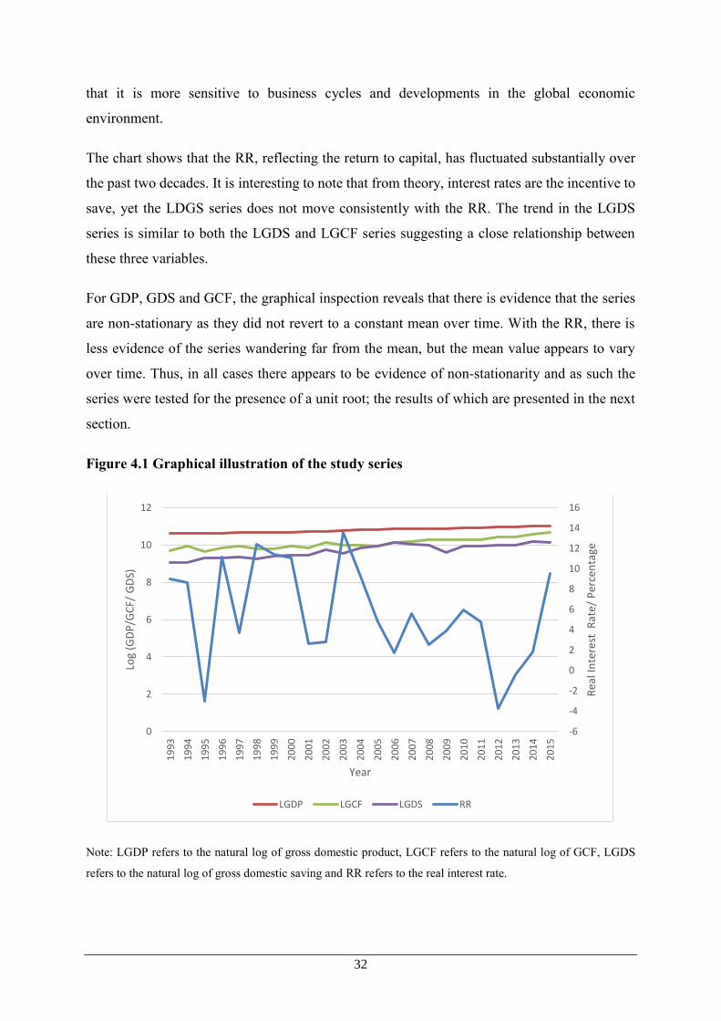
32

that it is more sensitive to business cycles and developments in the global economic

environment.

The chart shows that the RR, reflecting the return to capital, has fluctuated substantially over

the past two decades. It is interesting to note that from theory, interest rates are the incentive to

save, yet the LDGS series does not move consistently with the RR. The trend in the LGDS

series is similar to both the LGDS and LGCF series suggesting a close relationship between

these three variables.

For GDP, GDS and GCF, the graphical inspection reveals that there is evidence that the series

are non-stationary as they did not revert to a constant mean over time. With the RR, there is

less evidence of the series wandering far from the mean, but the mean value appears to vary

over time. Thus, in all cases there appears to be evidence of non-stationarity and as such the

series were tested for the presence of a unit root; the results of which are presented in the next

section.

Figure 4.1 Graphical illustration of the study series

Note: LGDP refers to the natural log of gross domestic product, LGCF refers to the natural log of GCF, LGDS

refers to the natural log of gross domestic saving and RR refers to the real interest rate.

-6

-4

-2

0

2

4

6

8

10

12

14

16

0

2

4

6

8

10

12

19

93

19

94

19

95

19

96

19

97

19

98

19

99

20

00

20

01

20

02

20

03

20

04

20

05

20

06

20

07

20

08

20

09

20

10

20

11

20

12

20

13

20

14

20

15

Rea

l In

tere

st R

ate/

Per

cen

tage

Log

(GD

P/G

CF/

GD

S)

Year

LGDP LGCF LGDS RR

33

4.3 Unit Root Tests

As indicated in the preceding chapter, the ADF and PP tests were used to formally test for

stationarity. The study employed both tests because the two tests at times yield conflicting

results for the same data sets due to differences in approach to estimation. If the tests yield

conflicting results, this warrants further investigation into the asymptotic properties of the time

series using alternative unit root tests. The stationarity tests are conducted using a constant

variable and then a trend variable is added to the tests to ensure robustness of results since the

data in this series can exhibit a trend.

The decision rule for both the ADF and PP tests is that we reject the null hypothesis of a unit

root if the tau statistic is more negative than the critical value. The results from the unit root

tests are presented in table 4.1. The results show that in all cases, the calculated tau values are

less negative than the critical values. Thus, as shown in the last column of table 4.1, both the

ADF and PP tests indicate that all the series considered in this study are non-stationary in levels

and contain at least one unit root. As explained in the previous chapter, given this finding, the

first differences of the series were then examined to test for the presence of a unit root.

The unit root tests were conducted on the study variables in first difference. The results of the

unit root tests are shown in table 4.2. The results show that all the calculated tau statistics are

more negative than the critical values at the 5% level of significance. The conclusion is that the

null hypothesis is rejected for all the series in first difference and thus it can be concluded that

all the series in this study are stationary in first difference and hence are integrated of order one.

34

Table 4.1 Unit Root Tests in Levels

Variable in Levels Test Tau-Test Tau-Critical

Value (5%)

Conclusion

LGDS

PP

Intercept -1.367

-3.005

Non-stationary

Trend and

Intercept

-3.075 -3.633

ADF

Intercept -1.475 -3.005

Trend and

Intercept

-3.038 -3.633

LGCF

PP

Intercept 0.081 -3.005

Non-stationary

Trend and

Intercept

-3.487 -3.633

ADF

Intercept 1.104 -3.005

Trend and

Intercept

-3.527 -3.633

LGDP

PP

Intercept 1.657 -3.005

Non-stationary Trend and

Intercept

-3.551 -3.633

ADF

Intercept 1.608 -3.005

Trend and

Intercept -3.543 -3.633

RR

PP

Intercept -2.765 -3.005

Non-stationary Trend and

Intercept

1.234 -3.633

ADF

Intercept 0.097 -3.005

Trend and

Intercept

-2.789 -3.633

35

Table 4.2 Unit Root Tests in First Differences

Variable in First

Difference

Test Tau-Test Tau-Critical

(5%)

Conclusion

DLGDS

PP

Intercept -6.763

-3.012

Stationary Trend and

Intercept

-6.650 -3.645

ADF

Intercept -6.796 -3.012

Trend and

Intercept

-6.688 --3.645

DLGCF

PP

Intercept -8.981 -3.012

Stationary Trend and

Intercept

-18.472 -3.645

ADF

Intercept -8.330 -3.012

Trend and

Intercept

-6.013 -3.645

DLGDP

PP

Intercept -4.841 -3.012

Stationary Trend and

Intercept

-4.959 -3.645

ADF

Intercept -4.758 -3.012

Trend and

Intercept

-4.915 -3.645

DRR

PP

Intercept -10.693 -3.012

Stationary Trend and

Intercept

-8.957 -3.645

ADF

Intercept -4.458 -3.012

Trend and

Intercept

-4.117 -3.645

36

4.4 Lag Length Selection

The next step is to test for the existence of a long-run relationship using the Johansen

cointegration approach. However, before carrying out this test, which uses a VAR system of

equations, the correct lag specification of the VAR is required. The results from this test are

shown in Table 4.3.

Table 4.3 Appropriate lag selection

Lag LR FPE AIC SIC HQIC

0 NA 4.57E-05 1.358 1.558 1.397

1 104.422* 2.24e-07* -4.003* -3.007* -3.809*

2 16.156 3.23E-07 -3.872 -2.080 -3.522

3 7.466 1.14E-06 -3.338 -0.749 -2.833

*indicates lag order selected by the criterion Likelihood Ratio (LR): sequential modified LR test statistic (each

test at 5%); FPE: Final prediction error, AIC: Akaike information criterion, SIC: Schwarz information criterion,

HQIC: Hannan-Quinn information criterion.

The results show that the AIC selects an optimal lag length of one; the information criterion

which was deemed most appropriate for this study based on the sample size. However, it is of

value to note that this lag length was confirmed by the other two information criteria – HQIC

and SIC, while two other measures, the final prediction error (FPE) and the log-likelihood ratio

test (LR) also indicate the same lag length. This lag length was applied in the cointegration test

and VAR analysis in the next section.

4.5 Cointegration Tests

Time series may have a long-run equilibrium relationship even if they exhibit a stochastic trend

over time. Given that the unit root tests revealed that the data used in this study is non-

stationary, the Johansen cointegration test was used to test for the existence of a long-run

relationship. A lag length of one, as informed by the information criterion, was specified in the

Johansen cointegration test. The results of both the trace and maximum eigenvalue tests are

used to ensure that the inferences drawn about the existence of a long-run relationship are

robust.

37

Table 4.4: Trace Test and Maximum Eigenvalue Test at the 5% Significance Level

Trace Test Maximum Eigenvalue Test

Cointegrating

Equations Eigenvalue Statistic

Critical

Value Prob. Eigenvalue Statistic

Critical

Value Prob.

None * 0.787 71.013 47.856 0.000 0.787 34.074 27.584 0.006

At most 1 * 0.704 36.939 29.797 0.006 0.704 26.771 21.132 0.007

At most 2 0.329 10.168 15.495 0.268 0.329 8.780 14.265 0.305

At most 3 0.061 1.388 3.8415 0.239 0.061 1.388 3.841 0.239

For both the trace and maximum-eigenvalue tests, the first test has a null hypothesis that there

are no cointegrating relationships, with the alternative hypothesis for the trace test being that

there are more than zero relationships while that for the maximum-eigenvalue test is that there

is at least one cointegrating equation. The test statistics are compared with the critical values

and if the calculated statistics are higher than the test critical values, the null hypothesis is

rejected. As shown in the table, the maximum eigenvalue test statistic of 34.074 is greater than

the critical value of 27.584 thus revealing that the null hypothesis of no cointegration is rejected

and there is at least one cointegrating equation. This conclusion is further supported by the trace

test where the calculated statistic of 71.013 is also greater than the critical value (47.856). The

conclusion is that there is evidence of cointegration in the series.

A second test was then performed with the null hypothesis of one cointegrating relationship

against the alternative of more than one relationship (trace) or at least two (maximum-

eigenvalue). The results for these tests show that the test statistics for the maximum eigen value

test of 26.771 was greater than the critical value of 21.132. The results of the trace test were

also consistent with those from the maximum eigenvalue test as the statistic (36.939) is greater

than the critical value (29.797). The conclusion is that the null hypothesis of at most one

cointegrating equation is rejected.

Given that the first two hypotheses were rejected, a third test was performed with the null

hypothesis of two cointegrating vectors. The results above show that the maximum eigenvalue

test statistic (8.78) is less than the critical value (14.265). The results of the trace test confirm

the maximum eigenvalue test. The conclusion is that the null hypothesis of at most two

cointegrating equations cannot be rejected.

The results from the cointegration test show that the VECM is suitable for analysing the

relationship between GDS, GCF, RR and GDP rather than a VAR because the series are

cointegrated.

38

4.6 Econometric Model

4.6.1 Long Run Analysis

The VECM is included in Appendix 1. The coefficients of the cointegrating equation represent

the long-run relationship in the VECM. This can be written as follows:

𝐿𝐺𝐷𝑃 = 14.023 + 0.5043𝐿𝐺𝐶𝐹 + 0.0271𝑅𝑅 (5.1)

𝐿𝐺𝐷𝑆 = 1.354 + 1.0796𝐿𝐺𝐶𝐹 + 0.1659𝑅𝑅 (5.2) Given that these variables are non-stationary, the equations are spurious so it is not possible to

ascertain whether the relationships are significant, but the size and signs of the coefficients can

be interpreted. The first cointegrating relationship, equation 5.1, shows a long-run positive

relationship between GCF and GDP. Thus, for a 1% increase in investment, GDP increases by

0.5% and a 1% rise in the real interest rate will lead to a 0.03% increase in GDP. GDP is thus

seen to be quite sensitive to investment in the long-run and the positive relationship is consistent

with theory. Overall, the results show that investment does impact GDP over the long-run. The

figure above shows a positive relationship between interest rates and national income in the

long run. For every 1% increase in the RR, GDP increases by 0.02%.

The second cointegrating equation, shown in equation 5.2, shows that there is a positive

relationship between investment and saving, with a 1% increase in GCF, GDS increases by

1.08%. In addition, the results show a positive relationship between saving and the interest rate;

a 1% increase in the real interest rate increases saving by 0.17%. The results show that

investment and saving affect each other in the long-run. These findings are discussed in further

detail in section 4.7.

4.6.2 Short Run Analysis

The error correction components in the VECM represent the speed of adjustment to the

equilibrium. Typically, the error correction term should lie between zero and one and should

be negative in value (Brooks, 2008). The error correction equations in the VECM and 5.2 are

denoted by EC1 and EC2 respectively.

The short run relationship is a follow:

𝐷𝐺𝐷𝑃𝑡 = −0.12𝐸𝐶1𝑡−1 − 0.19𝐷𝐺𝐷𝑃𝑡−1 (5.3)

𝐺𝐷𝑆 = −0.15 − 0.78𝐸𝐶2𝑡−1 − 1.94𝐷𝐺𝐷𝑃𝑡−1 − 0.09𝐷𝐺𝐷𝑆𝑡−1 + 0.57𝐷𝐺𝐶𝐹𝑡−1 (5.4)

39

𝐺𝐶𝐹 = 0.15 − 0.13𝐸𝐶2𝑡−1 − 2.18𝐷𝐺𝐷𝑃𝑡−1 + 0.14𝐷𝐺𝐷𝑆𝑡−1 + 0.11𝐷𝐺𝐶𝐹𝑡−1 (5.5)

The equations above only include significant terms from the VECM estimation at 0.05 level of

significance. The error correction terms are only included when they are negative and have

values between 0 and 1 which is the significance criteria (Brooks, 2008). The results above

show the short-run relationships between the variables of interest. Equation 5.3 shows that GDP

is only explained by lagged values of GDP short run. Equation 5.2 shows that an increase in

1% in GCF results in an increase of 0.57% in GDS. The results show that 78% of the

disequilibrium in the long-run relationship between investment and saving is adjusted within

one year. This shows that disequilibrium is corrected for quickly.

Equation 5.5 shows that there is a short-run relationship between GCF and GDS. The results

show that an increase of 1% in saving results in an increase in investment of 0.14%. The VECM

analysis shows that EC2 adjusts 13% of the disequilibrium between investment, saving and

gross domestic product within one year which is relatively slow.

4.6.3 Granger Causality Tests

Table 4.5: Granger Causality Test

Dependant Variable in the Regression

Independent Variable DRR DLGCF DLGDP DLGDS

DRR n/a 0.4419 0.4587 0.7962

DLGCF 0.0832 n/a 0.9894 0.0061*

DLGDP 0.0102* 0.781 n/a 0.0319*

DLGDS 0.1679 0.0065* 0.5869 n/a

Values in the table represent corresponding p-values, * denotes significance at the 5% level.

Table 4.5 above shows the calculated p-values for the F-test of Granger causality. The results

show that lagged values of GDP Granger-cause the real interest rate. Of particular interest to

this study are the findings related to GDP and GCF. There is no evidence to suggest that lags

of the differenced RR explain GCF or GDP which thus refutes the hypothesis of MacKinnon

and Shaw (1973) that higher interest rates by encouraging saving, increase the volume of

available domestic credit, which increases investment and ultimately economic growth.

Similarly, no relationship is found between either GCF or GDS and GDP. Therefore, in contrast

with Domar’s (1946) model, saving and capital accumulation do not appear to be important

variables in explaining economic growth in Namibia. A bi-directional relationship is found

40

between GCF and GDS suggesting that lags of saving Granger cause domestic investment while

lags of domestic investment also Granger cause domestic saving. Lags of GDP are also

identified to Granger cause GDS while the RR has no causal relationship with saving in

Namibia. The impulse response functions discussed in the next subsection will establish

whether the causal relationship between variables is positive or negative as well as the

magnitude of these relationships.

4.6.4 Impulse Response Functions

Figure 4.2 Response of GCF to GDS

The chart above depicts the relationship between saving and additions to capital stock in

Namibia. The results show that there is no immediate response of GCF to a one standard

deviation shock to GDS, with the impact only felt one year after the shock with this response

positive. However, two periods after the shock, GCF declines with the effect tapering out

thereafter. The increases in GCF wears off after five years suggesting that the increase in saving

is completely absorbed in investment and consumption during that period. The above

relationship is consistent with prior expectations as saving in expected to be translated to

investment and also mirrors the finding observed in the Granger causality tests. The positive

relationship between saving and investment above is consistent with the results of Aghion,

Comin and Howitt (2009) who explored the question of whether a country can grow faster by

-.05

.00

.05

.10

.15

.20

1 2 3 4 5 6 7 8 9 10

Response of DLGCF to DLGDS

Year

DLGCF

41

saving more. The results of the study revealed a positive relationship between saving and

investment in developing countries.

Figure 4.3 Response of GDP to GCF

The figure above shows the response of GDP to a one standard deviation shock in GCF. While

there is a small initial response in GDP to the shock in GCF, the first notable impact on the

Namibian economy occurs one year after and results in a surprsing decrease in GDP. However,

two years after the shock, there is a substantial increase in GDP. This is consistent with

Keynesian theory which argues that demand side policies in the form of expansionary fiscal

policies may be used to pursue growth objectives. However, it is important to note that after

two years, the shock’s contribution to GDP wears off resulting in a decrease in GDP in year 4.

This might be evidence that financing of investment through external borrowing results in a

debt burden which results in a decrease in income growth. The difference in the results observed

from the impulse response functions and the Granger causality tests can possibly be attributed

to the fact that the response of GDP to GCF is not immediate and the Granger causality tests

only consider a one period lag; thus, the ipulse response functions demonstrate that there is a

relationship between economic growth and investment in Namibia. These results are consistent

with Vemar’s (2007) findings which revealed that there is a positive relationship between

investment and economic growth.

-.004

-.002

.000

.002

.004

.006

.008

.010

.012

1 2 3 4 5 6 7 8 9 10

Response of DLGDP to DLGCF

Year

DLGDP

42

Figure 4.4 Response of GCF to RR

The chart above shows the response of GCF to an interest rate shock. The results show that a

one standard deviation shock in interest rates will only cause changes in investment after one

year and this response is very small. The results above show that an increase in interest rates

causes a transient increase in GCF which wears off after about ten years. These results are

consistent with the findings from the Granger causality test where no causality was found.

Figure 4.5 The Response of RR to GCF

-.05

.00

.05

.10

.15

.20

1 2 3 4 5 6 7 8 9 10

Response of DLGCF to DRR

Year

DLGCF

43

Figure 4.5 captures the relationship between the interest rate and GCF in Namibia. An increase

in GCF results in an increase in the real interest rate. This is consistent with the views of

McKinnon and Shaw (1973) who argued that high interest rates, by encouraging saving,

increase the volume of available domestic credit, which increases investment. The McKinnon

and Shaw hypothesis highlights that it is not the cost of financial resources that hinders

investment, but rather the lack of available financial resources for investment. The increase in

interest rates as a result of a one standard deviation shock on GCF is sustained over a long

period of time. This suggests that interest rates are sticky downwards. Research has shown that

markets are quick to increase interest rates in response to market forces (EPW Research

Foundation, 2009). Markets are however slow in adjusting to market forces that result in

decreases in interest rates. This might explain why increases in GCF cause a permanent increase

in interest rates over time.

Figure 4.6 Response of GDS to RR

-2

0

2

4

6

8

1 2 3 4 5 6 7 8 9 10

Response of DRR to DLGCF

Year

DRR

44

The line graph above tries to capture the impact of interest rates on saving in Namibia. The

chart shows like other shocks discussed earlier, an interest rate shock only impacts on saving

after one year. The results show that after the first year, there is an increase in saving. The

increase in saving after an increase in the interest rate decreases after year two and wears off

near the steady state after about 6 years. This is consistent with the Keynesian theory which

highlights that economic agents face liquidity constraints which constrain long-term saving

behaviour (Keynes, 1936). The small positive relationship between saving and interest rates

documented here, along with the absence of a relationship identified in the Granger causality

tests is consistent with empirical findings by Ogbokor (2014) who, using the VECM

methodology, examined the determinants of saving in Namibia and found that the deposit rate

has no effect on long term saving behaviour in Namibia.

4.6.5 Variance Decomposition

Variance decomposition was conducted on GCF first to reveal whether an increase in national

saving would lead to an increase in investment. Furthermore, variance decomposition on GDP

was also conducted to examine the relationship between investment and economic growth in

Namibia.

Table 4.6: Variance Decomposition of GCF

-.20

-.15

-.10

-.05

.00

.05

.10

.15

.20

1 2 3 4 5 6 7 8 9 10

Response of DLGDS to DRR

Year

DLGDS

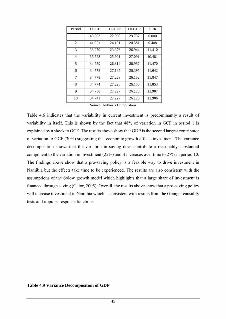
45

Period DGCF DLGDS DLGDP DRR

1 48.203 22.060 29.737 0.000

2 41.021 24.191 24.381 0.408

3 38.270 23.376 26.944 11.410

4 36.528 25.901 27.091 10.481

5 34.759 26.814 26.957 11.470

6 34.778 27.185 26.395 11.642

7 34.778 27.223 26.152 11.847

8 34.774 27.223 26.150 11.853

9 34.738 27.227 26.128 11.907

10 34.741 27.227 26.126 11.906

Source: Author’s Compilation

Table 4.6 indicates that the variability in current investment is predominantly a result of

variability in itself. This is shown by the fact that 48% of variation in GCF in period 1 is

explained by a shock to GCF. The results above show that GDP is the second largest contributor

of variation to GCF (30%) suggesting that economic growth affects investment. The variance

decomposition shows that the variation in saving does contribute a reasonably substantial

component to the variation in investment (22%) and it increases over time to 27% in period 10.

The findings above show that a pro-saving policy is a feasible way to drive investment in

Namibia but the effects take time to be experienced. The results are also consistent with the

assumptions of the Solow growth model which highlights that a large share of investment is

financed through saving (Galor, 2005). Overall, the results above show that a pro-saving policy

will increase investment in Namibia which is consistent with results from the Granger causality

tests and impulse response functions.

Table 4.9 Variance Decomposition of GDP

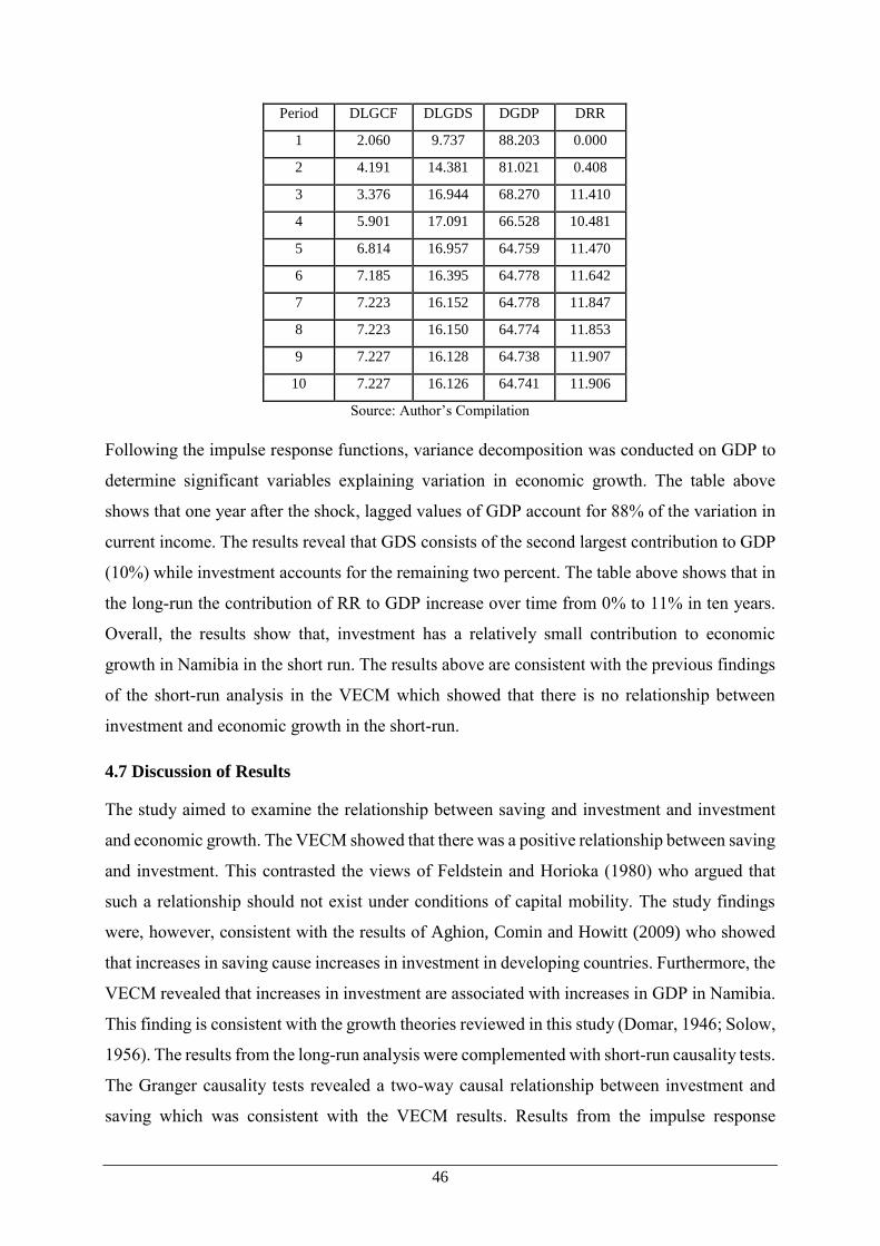
46

Period DLGCF DLGDS DGDP DRR

1 2.060 9.737 88.203 0.000

2 4.191 14.381 81.021 0.408

3 3.376 16.944 68.270 11.410

4 5.901 17.091 66.528 10.481

5 6.814 16.957 64.759 11.470

6 7.185 16.395 64.778 11.642

7 7.223 16.152 64.778 11.847

8 7.223 16.150 64.774 11.853

9 7.227 16.128 64.738 11.907

10 7.227 16.126 64.741 11.906

Source: Author’s Compilation

Following the impulse response functions, variance decomposition was conducted on GDP to

determine significant variables explaining variation in economic growth. The table above

shows that one year after the shock, lagged values of GDP account for 88% of the variation in

current income. The results reveal that GDS consists of the second largest contribution to GDP

(10%) while investment accounts for the remaining two percent. The table above shows that in

the long-run the contribution of RR to GDP increase over time from 0% to 11% in ten years.

Overall, the results show that, investment has a relatively small contribution to economic

growth in Namibia in the short run. The results above are consistent with the previous findings

of the short-run analysis in the VECM which showed that there is no relationship between

investment and economic growth in the short-run.

4.7 Discussion of Results

The study aimed to examine the relationship between saving and investment and investment

and economic growth. The VECM showed that there was a positive relationship between saving

and investment. This contrasted the views of Feldstein and Horioka (1980) who argued that

such a relationship should not exist under conditions of capital mobility. The study findings

were, however, consistent with the results of Aghion, Comin and Howitt (2009) who showed

that increases in saving cause increases in investment in developing countries. Furthermore, the

VECM revealed that increases in investment are associated with increases in GDP in Namibia.

This finding is consistent with the growth theories reviewed in this study (Domar, 1946; Solow,

1956). The results from the long-run analysis were complemented with short-run causality tests.

The Granger causality tests revealed a two-way causal relationship between investment and

saving which was consistent with the VECM results. Results from the impulse response

47

functions were consistent with the VECM results as they revealed that a saving innovation

results in transient increases in investment. In addition, the impulse response functions showed

that investment innovations are associated with increases in economic growth. This was in

contrast with the Granger causality test which showed that there was no causal relationship

between GCF and GDP. The differences in results can be attributed to the fact that the Granger

causality tests only included one lag whereas the relationship appears to take longer to manifest

as the impulse response functions and variance decompositions showed. Finally, variance

decomposition was conducted on GDP and GCF. This was done to understand whether Namibia

can achieve economic growth by saving more. The variance decomposition showed a strong

link between saving and investment but a weak link between investment and economic growth.

These results are consistent with findings from the Granger causality tests. Overall, the results

show that even though a pro-saving policy can drive investment levels in Namibia, it takes a

longer time period for the investment to increase gross domestic product as revealed by the long

run relationship between GCF and GDP.

4.8 Summary

This chapter presented the findings from the empirical analysis. The relationship between

saving and investment was found to be consistent with the findings by Aghion, Comin and

Howitt (2009) who revealed that saving had a positive effect on investment in developing

countries. Furthermore, the analyses showed that there is only a long run relationship between

investment and economic growth in Namibia. The next chapter concludes this study based on

the research findings.

48

5. RESEARCH CONCLUSIONS

5.1 Conclusions

This study examined the interaction between saving, investment and economic growth in

Namibia. The specific objectives of the study were to investigate the causal relationship

between saving and investment in Namibia. Furthermore, the study sought to reveal the impact

of the saving-investment relationship on economic growth in the country.

The study utilised GCF, GDS, GDP and the real interest rate. The diagnostic testing using the

Johansen cointegration test revealed a long-run relationship between the study variables with

two cointegrating equations. The VECM analysis showed that there is a long run relationship

between GDS and GCF. The second run relationship exists between GDP and GCF. The long-

run analysis was followed by a causal analysis using the Granger causality test. The tests

revealed that there was a bi-causal relationship between GDS and GCF. Furthermore, a causal

relationship between GCF and GDS was also identified. This relationship is one way with GDS

Granger causing GCF. To determine whether the relationship between variables is positive or

negative, impulse responses were estimated from the VECM model.

The impulse response analysis showed that GCF has a positive impact on national income in

the first two years. However, the effect of GCF on income growth steadily decreases and results

in reduced income growth after a period of about three years. This is associated with increased

debt burden and low returns from public infrastructure which is typical of public investment in

Namibia. The results are consistent with the Granger causality test which showed there is no

causal relationship between GCF and GDP.

Insights from the impulse response functions show that there is a sustained positive contribution

of GDS to GDP. This may be attributed to the fact that GDS is mostly private saving. This is

because the government has operated on a sustained budget deficit since 2010. Private savings

are mostly channelled towards more productive investments, hence this results in increased

national income. This was consistent with the Granger causality analysis which showed that

there was a causal relationship between GDS and GCF.

The study concludes that there is a causal relationship between GCF and GDS in Namibia. The

decrease in savings’ contribution to investment over time is consistent with growth theory.

According to the Solow growth model, increases in capital stock wear off over time due to

49

capital depreciation hence in the absence of further additions in the capital stock, the

contribution of saving to capital formation reduces over time (Galor, 2005).

The study also concludes that based on the VECM analysis, there is a positive relationship

between investment and economic growth in Namibia. Based on the VECM, impulse response

analysis and variance decomposition the study concludes that there is no short run relationship

between investment and economic growth.

5.2 Recommendations

Given the results discussed in the previous chapter and the conclusions, the study recommends

that to achieve economic growth, there is need to implement policies that encourage long term

investment in Namibia. This is achieved through encouraging the acquisition of capital goods

through giving duty exemptions on capital goods. In addition, tax exemptions can be offered to

strategic sectors of the economy to encourage investment in such sectors.

Overall, a pro-saving policy is effective in achieving economic growth in Namibia, the

government can implement policies that give incentives to saving. This can be achieved through

tax relief for individuals who save in long term financial products such as pension funds. Given

the relatively low levels of education in Namibia, compared to other countries in the region,

provision of financial education through financial literacy initiatives would be effective in

mobilising saving.

The relationship between GCF and real interest rate shows that increases in GCF causes

increases in RR. Higher interest rates imply that higher costs of borrowing have negative long

run effects on GCF. The implication is that depending on the way investment is financed, there

might be long run negative effects on growth because of debt financed infrastructural spending.

It is therefore recommended that government encourages market driven approaches to pursue

economic growth. This can be done through promoting private sector participation in

infrastructural investment, thus reducing the debt burden on the economy

5.3 Recommendations for future research

Given the findings of the study, the researcher recommends a detailed analysis of the effects of

different deficit regimes on economic growth in Namibia. This would shed light on the

effectiveness of predominantly Keynesian economic policies implemented by the Namibian

government, which is coming at a cost of a widening budget deficit. A detailed cost-benefit

50

analysis of government infrastructural spending and cost of servicing debt is therefore required

to establish if the country will meet its vision 2030 target.

51

REFERENCES

African Development Bank. (2014). Namibia Country Strategy Paper 2014-20.

Aghion, P., Comin, D. & Howitt, P. (2009). When Does Domestic Saving Matter for Economic

Growth? Journal of Economic Literature, 7(4): 34-42.

Atangana, I. (2015). Savings-Investment Relationship in Cameroon: Vector Auto Regressive

Analysis. International Journal of Humanities, Arts and Social Sciences, 2(3): 33-43.

Adeniyi, O. & Egwaikhide, F. (2013). Saving-Investment Nexus in Developing Countries:

Does Financial Development Matter? Journal of Economic Development, 119(38): 56-

78.

Roudet, S., Lahreche, A., & Zaher, M. (2016). Investment and Growth in the Arab World.

International Monetary Fund Scoping Note.

(https://www.imf.org/external/np/pp/eng/2016/050216.pdf

Bank of Namibia. (2004). Namibia Macroeconomic Model. Accessed April 21, 2017, from

https://www.bon.com.na%2fPublications%2fOther-Publications%2fOccasional-

Papers.aspx%3fpage%3d2&p=DevEx,5072.

Bank of Namibia. (2015). The Structure and Nature of Savings in Namibia. Accessed April 21,

2017, from: https://www.bon.com.na%2f&p=DevEx,5064.

Barro, D. (1974). On the Determination of the Public Debt. Journal of Political Economy,

87(7): 240- 271.

Bennion, E.G. (1945). The multiplier, the acceleration principle and fluctuating autonomous

investment. Review of Economic Statistics, 56(2): 67-78.

Berndt, E. (1990). The practice of econometrics: Classic and contemporary. MIT. Reading,

Massachusetts.

Bernheim, D. (1989). A Neoclassical Perspective on Budget Deficits. Journal of Economic

Perspectives, 3(2): 55-72.

Blanchard, O. & Johnson, D.R. (2013). Macroeconomics. Boston: Pearson.

Brooks, C. (2008). Introductory econometrics for finance. Cambridge: Cambridge University

Press.

52

Brue, S.L., McConnell, C.R., & Fynn, S.L. (2014). Essentials of Economics. New York:

McGraw Hill.

Burnham, K.P., Anderson, D.R., & Huyvaert, K.P. (2011). AIC model selection and

multimodel inference in behavioral ecology. Behavioral Ecology and Sociobiology, 65

(1): 23 –35.

Campa, J.M., & Goldberg, L. S. (1999). Investment, Pass-Through and Exchange Rates: A

Cross-Country Comparison. International Economic Review, 40 (2): 287-314.

Chen, G. (2009). Granger Causality via Vector Auto-Regression Tuned for FMRI Data

Analysis. Proceedings of the International Society for Magnetic Resonance in Medicine

Scientific Meeting and Exhibition, 23(4): 32-45.

Chibber, A., & Wijnbergen, S.V. (1992). Public Policy and Private Investment in Turkey.

World Bank Working Paper Series 27.

Clark, J. (1917). Business Acceleration and the Law of Demand: A Technical Factor in

Economic Cycles. Journal of Political Economy, 25(1): 217-235.

Corbo, V., & Schmidt-Hebbel, K. (1991). Public policies and saving in developing countries.

Journal of Development Economics, 36(1): 89-11.

Commendatore, P., Panico, C., & Pinto, A. (2011). Government Spending, Effective Demand,

Distribution and Growth: A Dynamic Analysis. Institutional and Social Dynamics of

Growth and Distribution. Metroeconomica, 62(1): 1–23.

Cyrille, S.M. (2010). Saving-Investment Correlation and Capital Mobility in Sub-Saharan

African Countries: A Reappraisal through Inward and Outward Capital Flows’

Correlation. International Journal of Economics and Finance, 2(2): 18-24.

Dritsaki, C. (2015). The long-run relationship between savings and investments in Greece.

International Journal of Economics and Finance, 7(9): 15-21.

Duesenberry, J.S. (1949). Income, Saving and the Theory of Consumer Behavior. Cambridge,

MA: Harvard University Press.

Edwards, S. (1992). Trade orientation, distortions and growth in developing countries. Journal

of Development Economics, 39(1): 31-57.

53

Engle, R.F., & Granger, C.W.J. (1987). Co-integration and Error Correction: Representation,

Estimation and Testing. Econometrica, 55(2): 251-276.

EPW Research Foundation. (2009). Sticky Lending Rates. Economic and Political Weekly

Journal. 44(25): 25-33.

Feldstein, M., & Horioka C. (1980). Domestic Saving and International Capital Flows. The

Economic Journal. 90(358): 314-329.

Fischer, S. (1993). Debt Deflation Theory of Great Depressions. Econometrica, 1:77-57.

Flassbeck, H. (2012). Savings, investment and growth: theory and reality. G-24 Policy Brief

No. 35.

Friedman, M. (1978). Crowding Out or Crowding in: Economic Consequences of Financing

Government Deficits. Brookings Papers on Economic Activity, 3(23):593-642.

Friedman, M. (1957). The Permanent Income Hypothesis: A Theory of the Consumption

Function. Princeton University Press. .

Friedman, M. (1957). Studies in the Quantity Theory of Money. Economica, 24(96): 366-372.

Gardner, B.L. (2005). Causes of rural economic development. Agricultural Economics, 32(1):

21-41.

Galor, O. (2005). From Stagnation to Growth: Unified Growth Theory. Journal of Economic

Literature. 1(1):171-293.

Getty, G. (2010). Growth of Total Capital. Accessed from:

https://www.ifalstaff.com/neweconomics/index.php/board,2.0.html

Greene, J., & Villaneuva, D. (1991). Private Investment in Developing Countries: An Empirical

Analysis. IMF Staff Papers, 38(1): 33-58.

Greenwood, J., & Jovanovic, B. (1990). Financial Development, Growth, and the Distribution

of Income. Journal of Political Economy. 98 (5): 1076-1107.

Guo, D., Dall’erba, S., & Gallo, J. L. (2013). The leading role of manufacturing in China’s

regional economic growth: A spatial econometric approach of Kaldor’s

laws. International Regional Science Review, 36(2): 139-166.

54

Guterez, C., Souza, R., & GuillÈn, O. (2007). Selection of Optimal Lag Length in Cointegrated

VAR Models with Weak Form of Common Cyclical Features. Journal of Economic

Literature, 32(53): 1-24.

Henrikson, K., & Herzog, R. (2015). Saving-Investment: A Spacey Relationship. The Journal

of Business Inquiry, 14(2155): 53-78.

Hull, J.C. (2015). Options, Futures and other Derivatives. Pearson: Boston.

Ilegbinosa, A., Abuo, M., & Ipalibo, S. (2015). Domestic Investment and Economic Growth

in Nigeria from 1970-2013: An Econometric Analysis. Canadian Social Science, 11(6):

70-79.

Johansen, S., & Juselius, S.G. (1990). Maximum Likelihood Estimation and Inference on

Cointegration, with Applications to the Demand for Money. Oxford Bulletin for

Economics and Statistics, 55(2): 169-184.

Jorgenson, D., & Hall, R. (1967). Tax Policy and Investment Behaviour. American Economic

Review, 57(7): 33-41.

Kaya, H. (2010). Saving Investment Association in Turkey. Journal of Economic Literature,

45(23):.34-42.

Kayıkçı, F. (2012). Saving Investment Correlations and Capital Mobility: Evidence from

Transition Economies. International Journal of Social Sciences and Humanity Studies,

4(2): 1309-1321.

Keating, J. (1992). Structural Approaches to Vector Auto-regressions. Federal Reserve Bank

Working Papers, 37-57.

Keynes, J.M. (1936). The General Theory of Employment. Quarterly Journal of Economics,

51(7): 209-23.

Khumalo, J. (2014). Interest Rate: Private Capital Formation Nexus in South Africa: Bounds

Test Approach. Mediterranean Journal of Social Sciences, 5(1): 22-13.

Kohl, R., & O'Brien, P. (1998). The Macroeconomics of. Ageing, Pensions and Savings: A

Survey. OECD Working Papers No 200.

Kopcke, R.W. (1985). The Determinants of Investment Spending. New England Economic

Review, 23(7): 19-35.

55

Krueger, A. (1978). Liberalization Attempts and Consequences (1978). National Bureau of

Economic Research.

Levine, R., & Renelt, D. (1992). A Sensitivity Analysis of Cross-Country Growth Regressions.

American Economic Review, 82(1): 942-963.

Lütkepohl, H., Saikkonen, P., & Trenkler, C. (2001). Maximum eigenvalue versus trace tests

for the cointegrating rank of a VAR process, The Econometrics Journal. 4(2): 287-310.

Mannor, D. (2014). Effective Spending: The Case of Infrastructure. Journal of Development

Economics, 41(8): 13-26.

Manueal, M. (2004). Political Models of Budget Deficits: a literature review.

PinhoInvestigação Trabalhos em curso. 138 (23): 1645-1738.

Mataya, S.C., & Veeman, M.M. (1996): The Behaviour of Private and Public Investment in

Malawi. The Canadian Journal of Economics, 29: 438-442.

McKinnon, R.I., & Shaw, E. (1973). Money and Capital in Economic Development.

Washington DC: The Brookings Institution.

Mehanna, R.A. (2003). The Temporal Causality between Investment and Growth in

Developing Economies. Journal of Business and Economics Research, 1(3): 13-26.

Ministry of Finance. (2016). Budget 2015-2016. Accessed April 21, 2017, from

http://www.bing.com/cr?IG=34512D2D18774FDB99719673A3617488&CID=30E459

B99DB16C6D21B753D29C216DD5&rd=1&h=N97VxfX78a_uepHyzaCsP-

y2TXF0pxbqbaqyWDEimfI&v=1&r=http%3a%2f%2fwww.mof.gov.na%2fbudget-

2015-2016&p=DevEx,5128.1.

Mitchell, D. (2009). The Impact of Government Spending on Economic Growth Heritage

foundation.

Mitchell, D. J. (2005). The impact of government spending on economic growth. The Heritage

Foundation, 1813: 1-18.

Mishkin, F. (2009). The Economics of Money, Banking, and Financial Markets. Prentice Hall.

Mousa, N.Y.A. (2010). Monetary Policy and the Role of Exchange Rate a Case of Jordan

(Unpublished PhD thesis). University of Birmingham, United Kingdom.

56

Mwinga, M. (2012). Unemployment in Namibia: Measurement Problems, Causes & Policies.

First Capital research. Accessed April 21, 2017 from:

http://www.nmanamibia.com/fileadmin/user_upload/pdf/Unemployment_in_Namibia_

May_2012.pdf.

Namibia Statistics Agency (NSA) (2012). Namibia Household Income & Expenditure Survey

(NHIES) 2009/2010.

Tien, D. (2016). The Interrelationship Among Foreign Direct Investment, Domestic Investment

and Export In Vietnam: A Causality Analysis. Duong Hanh Tien Faculty of Commerce,

Da Nang University of Economics, Da Nang.

National Development Plan (NDP) 4. (2012). Accessed April 21, 2017 from

http://www.npc.gov.na/?page_id=202.

Ndikumana, L. (2000): Financial Determinants of Domestic Investment in Sub-Saharan Africa.

World Development, 28(7): 381-400.

Ndovorwi, B.E. (1997). Public Policy and Private Investment in Zimbabwe. University of

Zimbabwe, Harare.

Nikiforos, M. (2015). A Nonbehavioral Theory of Saving. Levy Economics Institute. Working

Paper No 844.

Nindi, A., & Odhiambo, A. (2014). Savings and investment in Malawi: A causality test.

Investment Management and Financial Innovations, 11(4): 14-28.

North, D.C. (1990). Institutions, Institutional Change, and Economic Performance. Cambridge

University Press: New York.

North, D.C., & Thomas, R.P. (1973). The Rise of the Western World: A New Economic History.

Cambridge University Press: Cambridge.

O'Brien, R.H (2013). Economics. Boston: Pearson.

Ogbokor, C.A., & Samahiya, O. M. (2014). A time series analysis of determinants of savings

in Namibia. Journal of Economics and Sustainable Development, 5(8): 52-64.

Organisation for Economic Co-operation and Development (OECD). 2012). Development Co-

operation Report 2012. Accessed April 21, 2017, from

http://www.oecd.org/dac/dcr2012.htm

57

Organisation for Economic Co-operation and Development (OECD). (2016). Tax Policy

Reforms in the OECD 2016. Annual Report.

Pagano, M. (1993). Financial Markets and Growth: An Overview. European Economic Review,

37 (1): 613-622.

Parkin, M. (2012). Macroeconomics. Boston: Addison-Wesley.

Patrick, L. (2017). Gross Domestic Savings in Namibia. Accessed April 21, 2017 from:

http://www.tradingeconomics.com/namibia/gross-domestic-savings-percent-of-gdp-wb-

data.html

Pesaran, M. H., & Shin, Y. (1998). Generalized Impulse Response Analysis in Linear

Multivariate Models. Economics Letter, 58(1): 17-29.

Pereira, A.M. (2001). On the effects of Public Investment on Private Investment: What Crowds

in What? Public Finance Review. 29(8):17-21.

Phillips, P., & Perron, P. (1988). Testing for Unit Root in Time Series Regression. Biometrica,

34(12): 116-137.

Said, E.S., & Dickey, A.D. (1984). Testing for Unit Root in Autoregressive- moving Average

models of unknown Order. Biometrika, 71(3): 599-607.

Saint-Paul, G. (1992). Technological choice, financial markets and economic development.

European Economic Review, 36(1992): 763-781.

Schelettwein, C. (2015). Budget Statement for 2015/2016 Financial Year. Windhoek: Ministry

of Finance.

Schmidt-Hebbel, K., & Servén, L. (1999). What Drives Private Saving Across the World?

Working Papers Central Bank of Chile 47. Central Bank of Chile.

Schmidt-Hebbel, K., Corbo, F., Vittorio, B., & Klaus, B. (1999). Public Policies and Saving in

Developing Countries. Journal of Development Economics, 36(1):89–115.

Sjö, B. (2008). Testing for unit roots and cointegration. Lectures in Modern Econometric Time

series Analysis.

Sloman, J., Wride, A., & Garratt, D. (2015). Economics. London: Pearson.

58

Solow, R.M. (1956). A contribution to the theory of economic growth. The Quarterly Journal

of Economics, 70(1): 65-94.

Smith, A. (1977). An Inquiry into the Nature and Causes of the Wealth of Nations. University

of Chicago Press.

Stiftung, B. (2014) Namibia Country Report. Gütersloh.

Stiglitz, J.E., & Walsh, C. E. (2006). Aggregate Expenditures and Income. In Economics. New

York: WW Norton and Company.

Stock, J.H., & Watson, M. W., (2001). Vector Auto-regressions. The Journal of Economic

Perspectives, 15(4): 115-120.

Tobin, J. (1969). A General Equilibrium Approach to Monetary Theory. Journal of Money,

Credit and Banking, 1 (1): 15–29.

Uanguta, E., & Shiimi, I.W. (2016). Namibia Financial Stability Report. Windhoek: Bank of

Namibia.

Uanguta, E., Haiyambo, E., Kadhikwa, G., & Chimana, S. (2017). The Structure and Nature of

Savings in Namibia. Khomas: Windhoek.

Ullah, I., Shah, M., & Khan, F.U. (2011) Domestic Investment, Foreign Direct Investment, and

Economic Growth Nexus: A Case of Pakistan. Economics Research International,

2014(1): 1-5.

Verma, R. (2007). Savings, investment and growth in India: An application of the ARDL

bounds testing approach. South Asia Economic Journal, 8(1): 87-98.

Waner, A. (2014). Public Investment as an Engine of Growth. IMF Working Paper WP/14/148.

Watson S. I., Ilegbinosa, I. A., & Micheal, A. (2015). Domestic Investment and Economic

Growth in Nigeria From 1970-2013: An Econometric Analysis. Canadian Social

Science, 11(6): 70-79.

Wong, M. (2012). Investment and Growth In Rich And Poor Countries. Working Paper 17788.

National Bureau of Economic Research.

Yanovsky, M. (1965). Social accounting systems. Transaction Publishers.

59

Zafar, A (2011). The Estimation of the Cointegration Relationship between Growth, Domestic

Investment and Exports: The Indian Economy. International Journal of Economics and

Finance, 3(4):11.

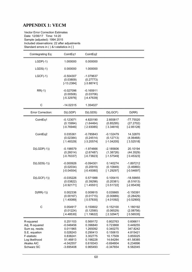
60

APPENDIX 1: VECM

Vector Error Correction Estimates Date: 12/06/17 Time: 14:20 Sample (adjusted): 1994 2015 Included observations: 22 after adjustments Standard errors in ( ) & t-statistics in [ ]

Cointegrating Eq: CointEq1 CointEq2 LGDP(-1) 1.000000 0.000000

LGDS(-1) 0.000000 1.000000

LGCF(-1) -0.504307 -1.079637 (0.03809) (0.27773) [-13.2384] [-3.88741]

RR(-1) -0.027096 -0.165911 (0.00508) (0.03706) [-5.32976] [-4.47639]

C -14.02315 1.354027 Error Correction: D(LGDP) D(LGDS) D(LGCF) D(RR) CointEq1 -0.123071 4.820190 2.855817 -77.75520 (0.15994) (1.64464) (0.85295) (27.2702) [-0.76946] [ 2.93085] [ 3.34816] [-2.85128]

CointEq2 0.035361 -0.785843 -0.132479 14.32870 (0.02384) (0.24514) (0.12713) (4.06468) [ 1.48329] [-3.20574] [-1.04205] [ 3.52518]

D(LGDP(-1)) -0.198579 -1.974666 -2.185606 20.10194 (0.26014) (2.67487) (1.38726) (44.3529) [-0.76337] [-0.73823] [-1.57549] [ 0.45323]

D(LGDS(-1)) -0.000926 -0.094301 0.140274 -1.897212 (0.02034) (0.20919) (0.10849) (3.46860) [-0.04554] [-0.45080] [ 1.29297] [-0.54697]

D(LGCF(-1)) -0.035226 0.571988 0.105415 -18.59955 (0.03822) (0.39298) (0.20381) (6.51613) [-0.92171] [ 1.45551] [ 0.51722] [-2.85439]

D(RR(-1)) 0.002336 0.009915 0.035665 -0.150391 (0.00167) (0.01715) (0.00889) (0.28429) [ 1.40089] [ 0.57830] [ 4.01092] [-0.52900]

C 0.054917 0.150602 0.152100 1.180192 (0.01224) (0.12590) (0.06529) (2.08756) [ 4.48530] [ 1.19622] [ 2.32947] [ 0.56535] R-squared 0.251103 0.569172 0.802763 0.606611

Adj. R-squared -0.048456 0.396840 0.723868 0.449255 Sum sq. resids 0.011965 1.265092 0.340275 347.8242 S.E. equation 0.028243 0.290413 0.150615 4.815421 F-statistic 0.838241 3.302775 10.17509 3.855025 Log likelihood 51.46813 0.198228 14.64284 -61.58385 Akaike AIC -4.042557 0.618343 -0.694804 6.234896 Schwarz SC -3.695408 0.965493 -0.347654 6.582045

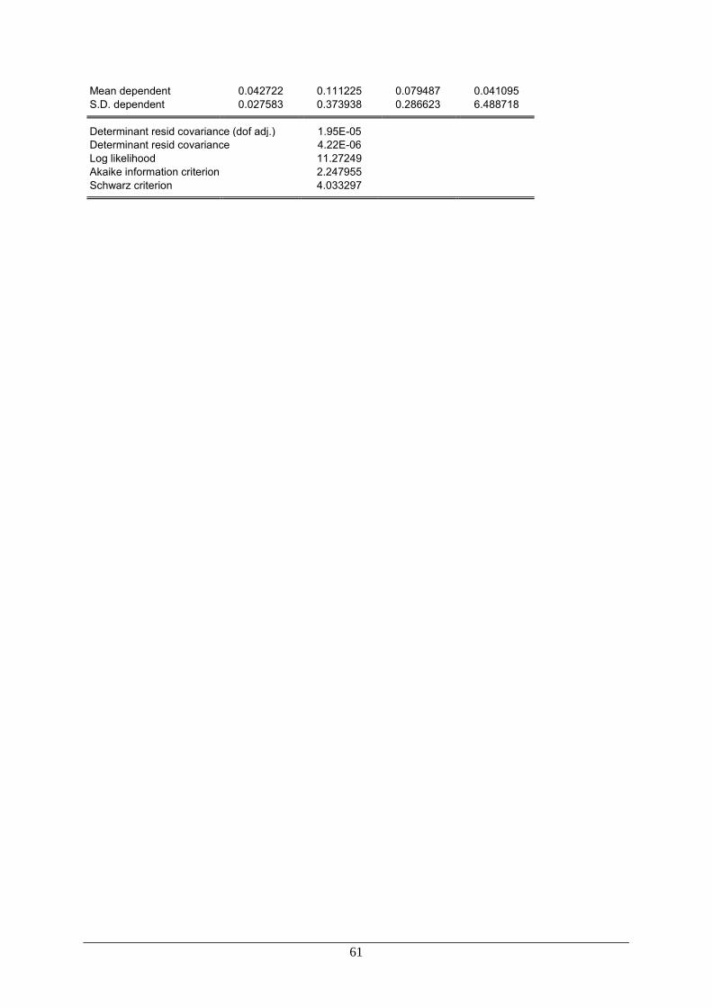
61

Mean dependent 0.042722 0.111225 0.079487 0.041095 S.D. dependent 0.027583 0.373938 0.286623 6.488718

Determinant resid covariance (dof adj.) 1.95E-05

Determinant resid covariance 4.22E-06 Log likelihood 11.27249 Akaike information criterion 2.247955 Schwarz criterion 4.033297