Savings in Location Management Costs Leveraging User Statistics
20
International Journal of UbiComp (IJU), Vol.2, No.3, July 2011 DOI:10.5121/iju.2011.2301 1 S AVINGS IN LOCATION M ANAGEMENT COSTS LEVERAGING USER S TATISTICS E. Martin and R. Bajcsy Department of Electrical Engineering and Computer Science University of California, Berkeley California, USA [email protected] A BSTRACT The growth in the number of users in mobile communications networks and the rise in the traffic generated by each user, are responsible for the increasing importance of Mobility Management. Within Mobility Management, the main objective of Location Management is to enable the roaming of the user in the coverage area. In this paper, we analyze the savings in Location Management costs obtained leveraging the users’ statistics, in comparison with the classical strategy. In particular, we introduce two novel algorithms to obtain the β parameters (useful terms in the calculation of location update costs for different Location Management strategies), utilizing a geographical study of relative positions of the cells within the location areas. Eventually, we discuss the influence of the different network parameters on the total Location Management costs savings for both the radio interface and the fixed network part, providing useful guidelines for the optimum design of the networks. K EYWORDS Mobility Management, Location Management, User statistics, Mobile Communications Networks. 1. INTRODUCTION Mobile communications networks operators need to solve difficult aspects regarding the mobility of the users and their interaction with the networks. Mobility Management is responsible for Handoff and Location Management. The former enables the continuation of a call while the user is on the move and changes cell, while the later enables the roaming of the user in the coverage area, with the main tasks involved being location update and paging [1-6]. The location update procedure consists of informing the network about every new location the mobile terminal enters, while paging is employed by the network to deliver incoming calls to the user. The signaling messages involved in these two procedures consume a significant proportion of the available radio resources [7-10]. In order to minimize this signaling burden, the location area concept (a set of cells) is used, whereby the mobile terminal will inform the network about a change in its position only when the location area’s border has been crossed. The employment of the call and mobility patterns of the user can help optimize the location area’s dimensions and minimize signaling costs [11]. In fact, mobile network operators often leverage handover statistics to improve the structure of their networks, with a strong impact on service performance and signaling load [12]. In this sense, user statistics-based algorithms for Location Management have proved to significantly reduce signaling costs [13-15]. In this type of algorithms, the most frequently visited location areas are assigned a probability coefficient consistent with the user’s residence time in each one of them. Subsequently, the network creates a list to order the location areas according to those probabilities, and in the case of an incoming call, the location areas will
-
Upload
ijujournal -
Category
Documents
-
view
222 -
download
0
Transcript of Savings in Location Management Costs Leveraging User Statistics
8/6/2019 Savings in Location Management Costs Leveraging User Statistics
http://slidepdf.com/reader/full/savings-in-location-management-costs-leveraging-user-statistics 1/20
International Journal of UbiComp (IJU), Vol.2, No.3, July 2011
DOI:10.5121/iju.2011.2301 1
S AVINGS IN LOCATION M ANAGEMENT COSTS
LEVERAGING USER S TATISTICS
E. Martin and R. Bajcsy
Department of Electrical Engineering and Computer ScienceUniversity of California, Berkeley
California, [email protected]
A BSTRACT
The growth in the number of users in mobile communications networks and the rise in the traffic generated
by each user, are responsible for the increasing importance of Mobility Management. Within Mobility Management, the main objective of Location Management is to enable the roaming of the user in the
coverage area. In this paper, we analyze the savings in Location Management costs obtained leveraging
the users’ statistics, in comparison with the classical strategy. In particular, we introduce two novel
algorithms to obtain the β parameters (useful terms in the calculation of location update costs for different
Location Management strategies), utilizing a geographical study of relative positions of the cells within the
location areas. Eventually, we discuss the influence of the different network parameters on the total
Location Management costs savings for both the radio interface and the fixed network part, providing
useful guidelines for the optimum design of the networks.
K EYWORDS
Mobility Management, Location Management, User statistics, Mobile Communications Networks.
1. INTRODUCTION
Mobile communications networks operators need to solve difficult aspects regarding the mobilityof the users and their interaction with the networks. Mobility Management is responsible forHandoff and Location Management. The former enables the continuation of a call while the useris on the move and changes cell, while the later enables the roaming of the user in the coveragearea, with the main tasks involved being location update and paging [1-6]. The location updateprocedure consists of informing the network about every new location the mobile terminal enters,while paging is employed by the network to deliver incoming calls to the user. The signalingmessages involved in these two procedures consume a significant proportion of the availableradio resources [7-10]. In order to minimize this signaling burden, the location area concept (a setof cells) is used, whereby the mobile terminal will inform the network about a change in itsposition only when the location area’s border has been crossed. The employment of the call and
mobility patterns of the user can help optimize the location area’s dimensions and minimizesignaling costs [11]. In fact, mobile network operators often leverage handover statistics toimprove the structure of their networks, with a strong impact on service performance andsignaling load [12]. In this sense, user statistics-based algorithms for Location Management haveproved to significantly reduce signaling costs [13-15]. In this type of algorithms, the mostfrequently visited location areas are assigned a probability coefficient consistent with the user’sresidence time in each one of them. Subsequently, the network creates a list to order the locationareas according to those probabilities, and in the case of an incoming call, the location areas will
8/6/2019 Savings in Location Management Costs Leveraging User Statistics
http://slidepdf.com/reader/full/savings-in-location-management-costs-leveraging-user-statistics 2/20
International Journal of UbiComp (IJU), Vol.2, No.3, July 2011
2
be paged sequentially following their decreasing order of probability. When the mobile user exitsthe predetermined set of location areas, it will perform a location update operation in the firstvisited cell. Therefore, a profile in the form of a list is needed for each user, containing theidentification of the most frequently visited location areas. In a simplified approach of thisalgorithm, only long term statistics (weeks or months) are memorized by the system, ignoringshort term statistics (hours or days). And even this basic approach considering only long termstatistics can bring important savings in location update operations. Recent examples making useof this approach can be found in reference [16], which describes an algorithm leveraging the userprofile history to reduce location update costs, utilizing cascaded correlation neural networkstrained on historical data of the user’s movements. This approach can be further improvedthrough the consideration of detailed data from the activity of the user, which can be extractedwith the sensors embedded in current state-of-the-art smart phones [17, 18].
In this paper, we analyze the savings in Location Management costs obtained leveraging theusers’ statistics, in comparison with the classical strategy. In particular, we introduce two novelalgorithms to obtain the β parameters (useful terms in the calculation of location update costs fordifferent Location Management strategies), utilizing a geographical study of relative positions of the cells within the location areas. Additionally, we discuss the influence of the different network
parameters on the total Location Management costs savings for both the radio interface and thefixed network part, providing useful guidelines for the optimum design of the networks.
The rest of this paper is organized as follows. In Section 2, we focus on the analysis of thelocation update costs for the user statistics-based algorithm and the classical strategy, making useof two new algorithms for the calculation of the β parameters. In Section 3, we analyze the pagingcosts for the user statistics-based algorithm and the classical strategy, while Section 4 is devotedto the study of the costs derived from maintaining the list of location areas managed by the userstatistics-based algorithm. In Section 5, we examine the total Location Management costs savingsof the user statistics-based algorithm in comparison with the classical strategy for both the radiointerface and the fixed network parts. Conclusions are drawn in Section 6.
2. CALCULATION OF LOCATION UPDATE COSTS
Assuming that a user of a mobile communications network follows a random movement and thatall the location areas under study have the same area, the frequency of the location updates willdepend on the speed of the mobile user [19-26], v, and the surface and perimeter length of thelocation areas [27-32]. Taking into account that the location update operations can take placewithin a same VLR (case 1, with probability 1 β ), or between two VLRs, making use of the
Temporary Mobile Subscriber Identity (case 2.1, with probability 21 β ), or making use of the
International Mobile Subscriber Identity (case 2.2, with probability 22 β ), the location updatecosts for the classical strategy in mobile communications networks with a two-tier architecturecan be expressed as follows [7-9]:
[ ])()()(8
_ 22cos,2221cos,211cos,1_ i Nbli Nbli Nbl
N R
vCost casecasecaseCSupdate ⋅+⋅+⋅⋅= β β β
π
(1)
Where R is the hexagonal cell side, N is the number of cells per location area, and )(cos, i Nbl case isthe number of bytes generated by a location update at interface i for any of the three differentcases explained before. Defining a parameter called 2 β as the probability of location update
using different VLRs, 21 β can be approximated by 80% of 2 β [33], and 22 β by 20% of 2 β . InSection 2.1, we will introduce two new algorithms for the calculation of these parameters.
8/6/2019 Savings in Location Management Costs Leveraging User Statistics
http://slidepdf.com/reader/full/savings-in-location-management-costs-leveraging-user-statistics 3/20
International Journal of UbiComp (IJU), Vol.2, No.3, July 2011
3
For a typical user statistics-based algorithm, also called “Alternative Strategy (AS)” by someauthors [7-8], the location update costs can be expressed as follows:
CSupdate
k
i
i ASupdate Cost Cost _
1
_ _1_ ⋅
−= ∑
=
α (2)
Where iα is the probability of finding a mobile user in the location area ai, and k is the number of location areas administered by this strategy.
2.1. Determination of the ββββ parameters
Assuming densely populated areas, with an average number of cells per location area of 10 [34],and an average number of location areas managed by a VLR of 5, the calculation of the β parameters to obtain the location update costs will be tackled next.
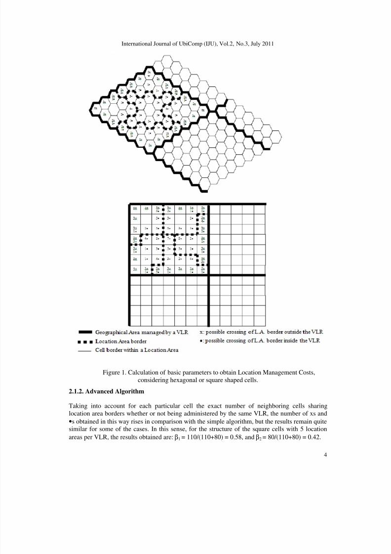
Different algorithms can be used to obtain the values for the β parameters. In this paper weanalyze the cells in the network one by one and determine the probabilities of a mobile terminalwith random movement entering a new location area, whether within the same VLR or not, so
that each cell is assigned a set of values, marked with a cross (denoted by “x”) or a dot (denotedby “•”) in Figure 1, to reflect respectively the probabilities of crossing the location area borderand moving outside the actual VLR administered zone or remaining within it. This approach canbe enhanced further leveraging the information obtainable from the sensors embedded in smartphones about the users’ location [5, 10, 15, 25], velocity [19, 21-24, 26], and activity [17-18].
The x and • numbers could be obtained through the mobile terminal’s mobility parameters ownedby the network operator, or through a geographical study of relative positions of the cells withinthe different location areas and the VLR administered zone itself. Considering this last option, thedifferent numbers assigned to each cell can be made dependant upon the designer’s criteria, forinstance in the two following ways: first, if the designer just wants to reflect the fact that a cell isneighboring a different VLR administered zone/location area, or second, if the designer wants toreflect the exact proportionality between the number of neighboring cells from a different VLRadministered zone and the number of neighboring cells from different location areas within thesame VLR administered zone. These two alternatives lead to a couple of methods that werespectively name simple and advanced algorithms.
2.1.1. Simple Algorithm
Taking for example a squared geographical area of dimensions 7·7=49 cells, so that the cellsadministered by a VLR can be grouped in 5 location areas with 10 cells each but one of them with9, considering that every cell in the border of the VLR administered zone as a whole can beassigned an x, and every cell sharing border with another location area within the same zone canbe assigned a •, the proportion between the number of •s and the sum of the number of xs and •swill represent the β1 parameter, while the proportion between the number of xs and the sum of thenumber of xs and •s will represent the β2 parameter. The results obtained for the referred
deployment are: β1 = 40/(40+24) = 0.625, and β2 = 24/(40+24) = 0.375.
Considering now the same VLR administered area but with lower number of cells per locationarea (9,7,6), so that the number of location areas increases to 6, the results obtained are verysimilar: β1=41/(41+24)=0.63 and β2=24/(41+24)=0.37. Now taking a VLR area composed of 7·7hexagonal cells, with 5 location areas of 11, 10 and 9 cells, the results obtained are:β1=34/(34+24)=0.59 and β2=24/(34+24)=0.41, similar to the previous case, although β2 becomesnoticeably larger.
8/6/2019 Savings in Location Management Costs Leveraging User Statistics
http://slidepdf.com/reader/full/savings-in-location-management-costs-leveraging-user-statistics 4/20
International Journal of UbiComp (IJU), Vol.2, No.3, July 2011
4
Figure 1. Calculation of basic parameters to obtain Location Management Costs,considering hexagonal or square shaped cells.
2.1.2. Advanced Algorithm
Taking into account for each particular cell the exact number of neighboring cells sharinglocation area borders whether or not being administered by the same VLR, the number of xs and•s obtained in this way rises in comparison with the simple algorithm, but the results remain quitesimilar for some of the cases. In this sense, for the structure of the square cells with 5 locationareas per VLR, the results obtained are: β1 = 110/(110+80) = 0.58, and β2 = 80/(110+80) = 0.42.
8/6/2019 Savings in Location Management Costs Leveraging User Statistics
http://slidepdf.com/reader/full/savings-in-location-management-costs-leveraging-user-statistics 5/20
International Journal of UbiComp (IJU), Vol.2, No.3, July 2011
5
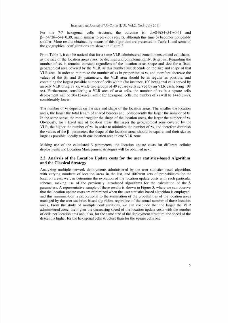
For the 7·7 hexagonal cells structure, the outcome is: β1=84/(84+54)=0.61 andβ2=54/(84+54)=0.39, again similar to previous results, although this time β2 becomes noticeablysmaller. More results obtained by means of this algorithm are presented in Table 1, and some of the geographical configurations are shown in Figure 2.
From Table 1, it can be noticed that for a same VLR administered zone dimension and cell shape,as the size of the location areas rises, β1 declines and complementarily, β2 grows. Regarding thenumber of xs, it remains constant regardless of the location areas shape and size for a fixedgeographical area covered by the VLR, as this number just depends on the size and shape of thatVLR area. In order to minimize the number of xs in proportion to •s, and therefore decrease thevalues of the β21 and β22 parameters, the VLR area should be as regular as possible, andcontaining the largest possible number of cells within (for instance, 100 hexagonal cells served byan only VLR bring 78 xs, while two groups of 49 square cells served by an VLR each, bring 108xs). Furthermore, considering a VLR area of m·m cells, the number of xs in a square cellsdeployment will be 20+12·(m-2), while for hexagonal cells, the number of xs will be 14+8·(m-2),considerably lower.
The number of •s depends on the size and shape of the location areas. The smaller the location
areas, the larger the total length of shared borders and, consequently the larger the number of •s.In the same sense, the more irregular the shape of the location areas, the larger the number of •s.Obviously, for a fixed size of location areas, the larger the geographical zone covered by theVLR, the higher the number of •s. In order to minimize the number of •s, and therefore diminishthe values of the β1 parameter, the shape of the location areas should be square, and their size aslarge as possible, ideally to fit one location area in one VLR zone.
Making use of the calculated β parameters, the location update costs for different cellulardeployments and Location Management strategies will be obtained next.
2.2. Analysis of the Location Update costs for the user statistics-based Algorithm
and the Classical Strategy
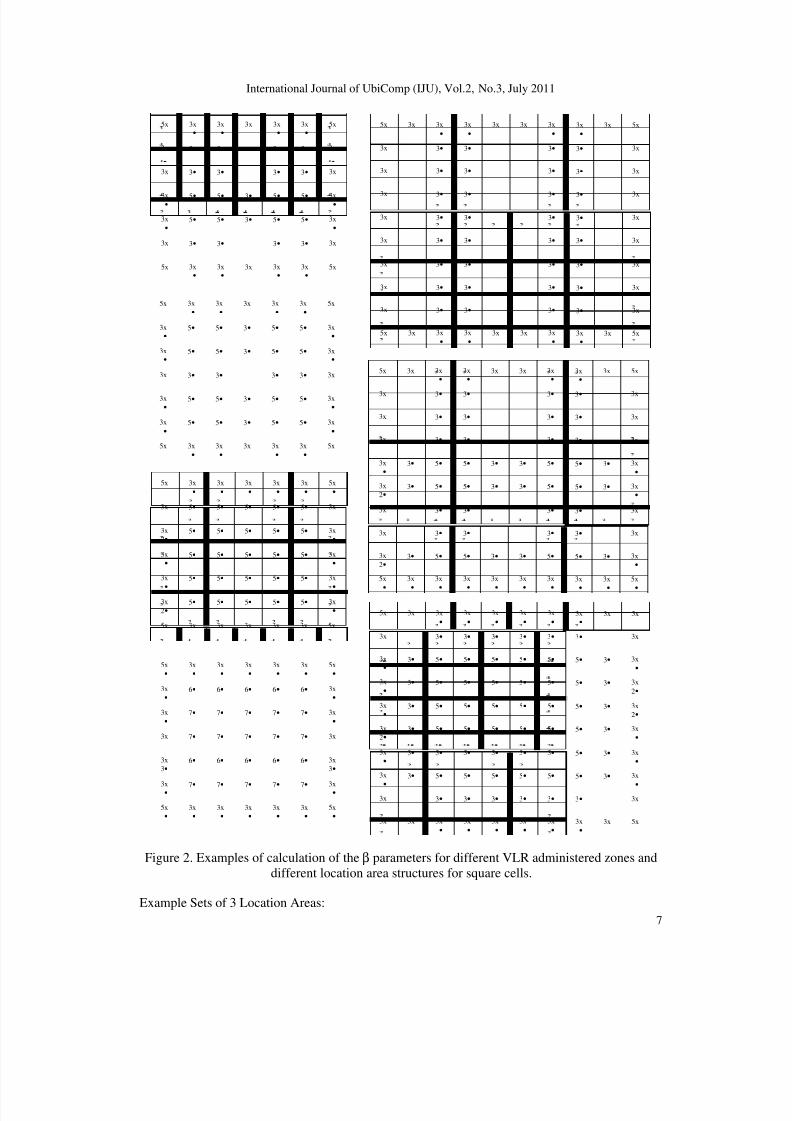
Analyzing multiple network deployments administered by the user statistics-based algorithm,with varying numbers of location areas in the list, and different sets of probabilities for thelocation areas, we can determine the evolution of the location update costs with each particularscheme, making use of the previously introduced algorithms for the calculation of the β parameters. A representative sample of these results is shown in Figure 3, where we can observethat the location update costs are minimized when the user statistics based algorithm is employed,and this minimization is proportional to the summation of the probabilities of the location areasmanaged by the user statistics-based algorithm, regardless of the actual number of those locationareas. From the study of multiple configurations, we can conclude that the larger the VLRadministered zone, the higher the decreasing speed of the location update costs with the numberof cells per location area and, also, for the same size of the deployment structure, the speed of thedescent is higher for the hexagonal cells structure than for the square cells one.
8/6/2019 Savings in Location Management Costs Leveraging User Statistics
http://slidepdf.com/reader/full/savings-in-location-management-costs-leveraging-user-statistics 6/20
International Journal of UbiComp (IJU), Vol.2, No.3, July 2011
6
Table 1. Calculation of β parameters for different network deployments.
Cell
Shape
VLR
administered
zone
dimension
Number
of L.A.s
per VLR
Number
of cells
per L.A.
Regularity
of shape of
L.A.s
No.
x
No.
••••
ββββ1 ββββ2 ββββ21 ββββ22
Hexagonal 7cells·7cells 5 9,10,11 Good 54 84 0.61 0.39 0.312 0.078
Hexagonal 7cells·7cells 4 9,12,16 Very good 54 50 0.48 0.52 0.416 0.104
Hexagonal 10cells·10cells 9 9,12,16 Very good 78 144 0.65 0.35 0.28 0.07
Hexagonal 10cells·10cells 4 25 Very good 78 74 0.49 0.51 0.408 0.102
Hexagonal 10cells·10cells 2 50 Very good 78 38 0.33 0.67 0.536 0.134
Square 7cells·7cells 17 2,3 Good 80 248 0.76 0.24 0.192 0.048
Square 7cells·7cells 16 1,2,4 Very good 80 191 0.7 0.3 0.24 0.06
Square 7cells·7cells 9 4,6,9 Very good 80 136 0.63 0.37 0.296 0.074
Square 7cells·7cells 6 6,8,9,12 Very good 80 106 0.54 0.41 0.328 0.082
Square 7cells·7cells 5 9,10 Medium 80 110 0.58 0.42 0.336 0.084
Square 7cells·7cells 4 9,12,16 Very good 80 72 0.47 0.53 0.424 0.106
Square 7cells·7cells 3 12,16,21 Good 80 50 0.38 0.62 0.496 0.124
Square 7cells·7cells 2 21,28 Very good 80 38 0.32 0.68 0.544 0.136
Square 10cells·10cells 33 3,4 Good 116 550 0.83 0.17 0.136 0.034
Square 10cells·10cells 16 4,6,9 Very good 116 300 0.72 0.28 0.224 0.056
Square 10cells·10cells 9 3,4,12,15 Good 116 208 0.64 0.36 0.288 0.072
Square 10cells·10cells 9 9,12,16 Very good 116 208 0.64 0.36 0.288 0.072
Square 10cells·10cells 4 25 Very good 116 108 0.48 0.52 0.416 0.104
Square 10cells·10cells 3 30,40 Very good 116 112 0.49 0.51 0.408 0.102
Square 10cells·10cells 2 50 Very good 116 56 0.33 0.67 0.536 0.134
8/6/2019 Savings in Location Management Costs Leveraging User Statistics
http://slidepdf.com/reader/full/savings-in-location-management-costs-leveraging-user-statistics 7/20
International Journal of UbiComp (IJU), Vol.2, No.3, July 2011
7
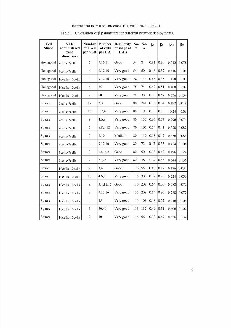
Figure 2. Examples of calculation of the β parameters for different VLR administered zones anddifferent location area structures for square cells.
Example Sets of 3 Location Areas:
5x 3x•
3x•
3x 3x•
3x•
5x
3x 3• 3• 3• 3• 3x
3x 3• 3• 3• 3• 3x
3x• 5• 5• 3• 5• 5• 3x
•
3x•
5• 5• 3• 5• 5• 3x•
3x 3• 3• 3• 3• 3x
5x 3x•
3x•
3x 3x•
3x•
5x
5x 3x•
3x•
3x 3x•
3x•
5x
3x•
5• 5• 3• 5• 5• 3x•
3x•
5• 5• 3• 5• 5• 3x•
3x 3• 3• 3• 3• 3x
3x•
5• 5• 3• 5• 5• 3x•
3x•
5• 5• 3• 5• 5• 3x•
5x 3x•
3x•
3x 3x•
3x•
5x
5x 3x•
3x•
3x•
3x•
3x•
5x•
3x 5• 5• 5• 5• 5• 3x
3x2•
5• 5• 5• 5• 5• 3x•
3x•
5• 5• 5• 5• 5• 3x•
3x
•
5• 5• 5• 5• 5• 3x
• 3x2•
5• 5• 5• 5• 5• 3x•
5x 3x 3x 3x 3x 3x 5x
5x•
3x•
3x•
3x•
3x•
3x•
5x•
3x•
6• 6• 6• 6• 6• 3x•
3x•
7• 7• 7• 7• 7• 3x•
3x 7• 7• 7• 7• 7• 3x
3x3•
6• 6• 6• 6• 6• 3x3•
3x• 7• 7• 7• 7• 7• 3x•
5x•
3x•
3x•
3x•
3x•
3x•
5x•
3x 3• 3• 3• 3• 3x
3x 3• 3• 3• 3• 3x
5x 3x 3x•
3x•
3x 3x 3x•
3x•
3x 5x
3x 3• 3• 3• 3• 3x
3x 3• 3• 3• 3• 3x
3x 3• 3• 3• 3• 3x
3x 3• 3• 3• 3• 3x
5x 3x 3x•
3x•
3x 3x 3x•
3x•
3x 5x
3x 3• 3• 3• 3• 3x
3x 3• 3• 3• 3• 3x
3x 3• 3• 3• 3• 3x
3x 3• 3• 3• 3• 3x
5x 3x 3x•
3x•
3x 3x 3x•
3x•
3x 5x
3x 3• 3• 3• 3• 3x
3x•
3• 5• 5• 3• 3• 5• 5• 3• 3x•
3x2•
3• 5• 5• 3• 3• 5• 5• 3• 3x•
3x2•
3• 5• 5• 3• 3• 5• 5• 3• 3x•
5x
•
3x
•
3x
•
3x
•
3x
•
3x
•
3x
•
3x
•
3x
•
5x
•
3x 3• 3• 3• 3• 3x
3x 3• 3• 3• 3• 3x
3x•
3• 5• 5• 5• 5• 5• 5• 3• 3x•
3x•
3• 5• 5• 5• 5• 5• 5• 3• 3x2•
5x 3x 3x•
3x•
3x•
3x•
3x•
3x•
3x 5x
3x 3• 3• 3• 3• 3• 3• 3x
3x•
3• 5• 5• 5• 5• 5• 5• 3• 3x2•
3x2•
3• 5• 5• 5• 5• 5• 5• 3• 3x•
3x 3• 3• 3• 3• 3• 3• 3x
5x 3x 3x•
3x•
3x•
3x•
3x•
3x•
3x 5x
3x•
3• 5• 5• 5• 5• 5• 5• 3• 3x•
3x
•
3• 5• 5• 5• 5• 5• 5• 3• 3x
•
8/6/2019 Savings in Location Management Costs Leveraging User Statistics
http://slidepdf.com/reader/full/savings-in-location-management-costs-leveraging-user-statistics 8/20
International Journal of UbiComp (IJU), Vol.2, No.3, July 2011
8
Probabilities: α1=0.4, α2=0.1, α3=0.05Probabilities: α1=0.5, α2=0.1, α3=0.05Probabilities: α1=0.6, α2=0.1, α3=0.05Probabilities: α1=0.7, α2=0.1, α3=0.05Probabilities: α1=0.8, α2=0.1, α3=0.05
Example Sets of 5 Location Areas:Probabilities: α1=0.4, α2=0.1, α3=0.05, α4=0.02, α5=0.01Probabilities: α1=0.5, α2=0.1, α3=0.05, α4=0.02, α5=0.01Probabilities: α1=0.6, α2=0.1, α3=0.05, α4=0.02, α5=0.01Probabilities: α1=0.7, α2=0.1, α3=0.05, α4=0.02, α5=0.01Probabilities: α1=0.8, α2=0.1, α3=0.05, α4=0.02, α5=0.01
Example Sets of 9 Location Areas:Probabilities: α1=0.4, α2=0.05, α3=0.03, α4=0.02, α5=0.01, α6=0.008, α7=0.005, α8=0.003, α9=0.002Probabilities: α1=0.5, α2=0.05, α3=0.03, α4=0.02, α5=0.01, α6=0.008, α7=0.005, α8=0.003, α9=0.002Probabilities: α1=0.6, α2=0.05, α3=0.03, α4=0.02, α5=0.01, α6=0.008, α7=0.005, α8=0.003, α9=0.002Probabilities: α1=0.7, α2=0.05, α3=0.03, α4=0.02, α5=0.01, α6=0.008, α7=0.005, α8=0.003, α9=0.002Probabilities: α1=0.8, α2=0.05, α3=0.03, α4=0.02, α5=0.01, α6=0.008, α7=0.005, α8=0.003, α9=0.002
10 20 30 40 50
7000
8000
9000
10000
11000
12000
Number of cells per location area
Bytes
Location Update Costs
10 20 30 40 500
1000
2000
3000
4000
5000
6000
7000
Number of cells per location area
Bytes
Location Update Costs
First Set o f Probabilities
Second Set of Probabilities
Third Set of Probabilities
Fourth Set of Probabilities
Fifth Set of Probabilities
a) Classical Strategy b) User Statistics and 3 Location Areas
10 20 30 40 500
1000
2000
3000
4000
5000
6000
7000
Number of cells per location area
Bytes
Location Update Costs
First Set of ProbabilitiesSecond Set of ProbabilitiesThird Set of Probabilities
Fourth Set of ProbabilitiesFifth Set of Probabilities
10 20 30 40 500
2000
4000
6000
8000
Number of cells per location area
Bytes
Location Update Costs
First Set of Probabilities
Second Set of Probabilities
Third Set of Probabilities
Fourth Set of Probabilities
Fifth Set of Probabilities
c) User Statistics and 5 Location Areas d) User Statistics and 3 Location Areas
Figure 3. Example of location update costs for the classical strategy and the user statistics-basedalgorithm considering different numbers of Location Areas managed.
The fact that hexagonal cells deliver lower location update costs than square cells (in agreementwith [2-4]) can be reasoned making use of the advanced algorithm for the calculation of the β parameters: the percentage reduction in the hexagonal cell structures with respect to the square
8/6/2019 Savings in Location Management Costs Leveraging User Statistics
http://slidepdf.com/reader/full/savings-in-location-management-costs-leveraging-user-statistics 9/20
International Journal of UbiComp (IJU), Vol.2, No.3, July 2011
9
cells structures is always higher for the number of xs than for the number of •s, as shown in Table2.
Table 2. Comparison of the percentage reduction of xs and •s in the advanced algorithm for thehexagonal cells with respect to the square cells.
VLR administered
zone size
No. Location
Areas
No. cells
per L. A.
Percentage of
reduction in x
Percentage of
reduction in ••••
10·10 9 11 32.76 30.7710·10 4 25 32.76 31.4810·10 2 50 32.76 32.147·7 5 10 32.5 23.637·7 4 11 32.5 30.55
Therefore, the hexagonal cells structures will present relatively lower values of β21 and β22, whichaccount for the highest terms in the location update costs, and consequently the costs will belower. However, from Table 2, it can be inferred that as the number of cells per location areaincreases, the difference in the percentage reduction between xs and •s tends to decline, andconsequently the reduction in the location update costs will diminish.
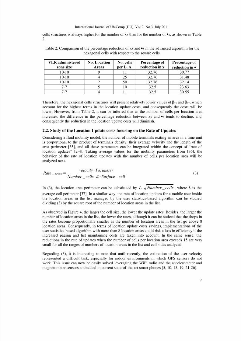
2.2. Study of the Location Update costs focusing on the Rate of Updates
Considering a fluid mobility model, the number of mobile terminals exiting an area in a time unitis proportional to the product of terminals density, their average velocity and the length of thearea perimeter [35], and all these parameters can be integrated within the concept of “rate of location updates” [2-4]. Taking average values for the mobility parameters from [36], thebehavior of the rate of location updates with the number of cells per location area will beanalyzed next.
cellSurfacecells Number
Perimeter velocity Rate update
___
⋅⋅
⋅=
π (3)
In (3), the location area perimeter can be substituted by cells Number L _⋅ , where L is the
average cell perimeter [37]. In a similar way, the rate of location updates for a mobile user insidethe location areas in the list managed by the user statistics-based algorithm can be studieddividing (3) by the square root of the number of location areas in the list.
As observed in Figure 4, the larger the cell size, the lower the update rates. Besides, the larger thenumber of location areas in the list, the lower the rates, although it can be noticed that the drops inthe rates become proportionally smaller as the number of location areas in the list go above 8location areas. Consequently, in terms of location update costs savings, implementations of theuser statistics-based algorithm with more than 8 location areas could risk a loss in efficiency if theincreased paging and list maintaining costs are taken into account. In the same sense, the
reductions in the rate of updates when the number of cells per location area exceeds 15 are verysmall for all the ranges of numbers of location areas in the list and cell sides analyzed.
Regarding (3), it is interesting to note that until recently, the estimation of the user velocityrepresented a difficult task, especially for indoor environments in which GPS sensors do notwork. This issue can now be easily solved leveraging the WiFi radio and the accelerometer andmagnetometer sensors embedded in current state-of-the-art smart phones [5, 10, 15, 19, 21-26].
8/6/2019 Savings in Location Management Costs Leveraging User Statistics
http://slidepdf.com/reader/full/savings-in-location-management-costs-leveraging-user-statistics 10/20
International Journal of UbiComp (IJU), Vol.2, No.3, July 2011
10
0 10 20 30 40 500
5
10
15
20
25
Number of cells per Location Area
u n
i t s / t i m e
Evolution of the rate of location updates
Cell side=0.15 KmCell side=0.30 Km
Cell side=0.45 KmCell side=0.60 Km
0 10 20 30 40 500
5
10
15
20
Number of cells per Location Area
u n
i t s / t i m e
Evolution of rate of location updates. Cell side=0.15km
2 Location Areas in the list4 Location Areas in the list6 Location Areas in the list8 Location Areas in the list10 Location Areas in the list12 Location Areas in the list
14 Location Areas in the list
a) Outside the L.A.s in the list b) Inside the list, cell side=0.15 km
0 10 20 30 40 500
2
4
6
8
10
Number of cells per Location Area
u n i t s /
t i m e
Evolution of rate of location updates. Cell side=0.30km
2 Location Areas in the list4 Location Areas in the list6 Location Areas in the list8 Location Areas in the list10 Location Areas in the list12 Location Areas in the list14 Location Areas in the list
0 10 20 30 40 500
1
2
3
4
5
6
Number of cells per Location Area
u n i t s / t i m e
Evolution of rate of location updates. Cell side=0.45km
2 Location Areas in the list4 Location Areas in the list6 Location Areas in the list8 Location Areas in the list10 Location Areas in the list12 Location Areas in the list14 Location Areas in the list
c) Inside the list, cell side=0.30 km d) Inside the list, cell side=0.45 km
Figure 4. Rate of location updates outside and inside the location areas in the list.
3. ANALYSIS OF THE PAGING COSTS
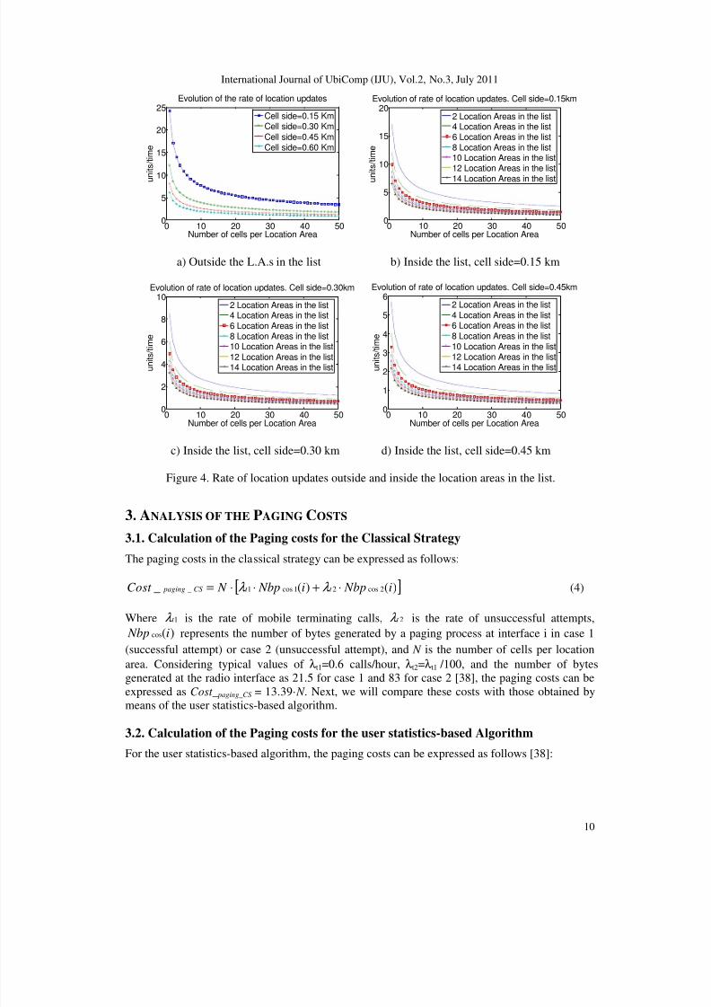
3.1. Calculation of the Paging costs for the Classical Strategy
The paging costs in the classical strategy can be expressed as follows:
[ ])()(_ 2cos21cos1_ i Nbpi Nbp N Cost t t CS paging ⋅+⋅⋅= λ λ (4)
Where 1t λ is the rate of mobile terminating calls, 2t λ is the rate of unsuccessful attempts,)(cos i Nbp represents the number of bytes generated by a paging process at interface i in case 1
(successful attempt) or case 2 (unsuccessful attempt), and N is the number of cells per locationarea. Considering typical values of λt1=0.6 calls/hour, λt2=λt1 /100, and the number of bytesgenerated at the radio interface as 21.5 for case 1 and 83 for case 2 [38], the paging costs can beexpressed as Cost_ paging_CS = 13.39· N . Next, we will compare these costs with those obtained by
means of the user statistics-based algorithm.
3.2. Calculation of the Paging costs for the user statistics-based Algorithm
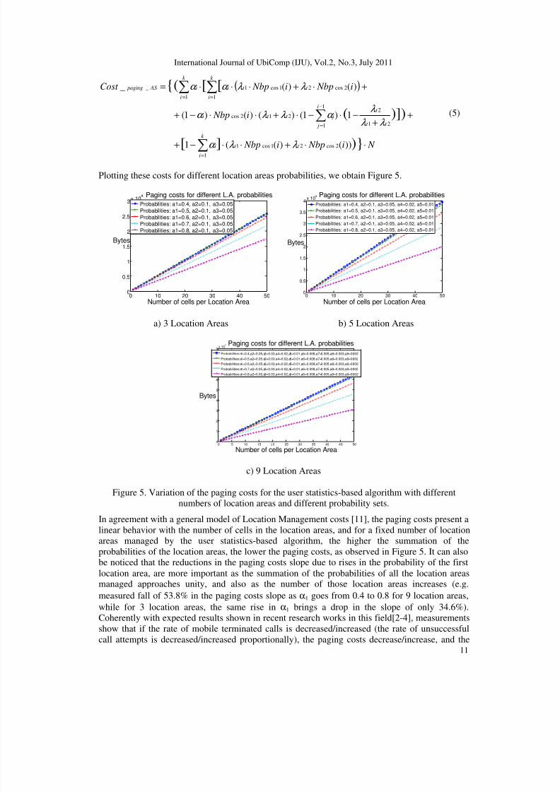
For the user statistics-based algorithm, the paging costs can be expressed as follows [38]:
8/6/2019 Savings in Location Management Costs Leveraging User Statistics
http://slidepdf.com/reader/full/savings-in-location-management-costs-leveraging-user-statistics 11/20
International Journal of UbiComp (IJU), Vol.2, No.3, July 2011
11
( )
∑
∑
∑ ∑
=
−
=
= =
⋅⋅+⋅⋅−+
++
−⋅−⋅+⋅⋅−+
+⋅+⋅⋅⋅=
k
i
t t i
i
j t t
t jt t i
k
i
k
i
t t ii AS paging
N i Nbpi Nbp
i Nbp
i Nbpi NbpCost
1
2cos21cos1
1
1 21
2212cos
1 1
2cos21cos1_
)}][
)])(
[[{(
))()((1
1)1()()()1(
)()(_
λ λ α
λ λ
λ α λ λ α
λ λ α α
(5)
Plotting these costs for different location areas probabilities, we obtain Figure 5.
0 10 20 30 40 500
0.5
1
1.5
2
2.5
3x 10
4
Number of cells per Location Area
Bytes
Paging costs for different L.A. probabilities
Probabilities: a1=0.4, a2=0.1, a3=0.05
Probabilities: a1=0.5, a2=0.1, a3=0.05
Probabilities: a1=0.6, a2=0.1, a3=0.05Probabilities: a1=0.7, a2=0.1, a3=0.05
Probabilities: a1=0.8, a2=0.1, a3=0.05
0 10 20 30 40 500
0.5
1
1.5
2
2.5
3
3.5
4x 10
4
Number of cells per Location Area
Bytes
Paging costs for different L.A. probabilities
Probabilities: a1=0.4, a2=0.1, a3=0.05, a4=0.02, a5=0.01
Probabilities: a1=0.5, a2=0.1, a3=0.05, a4=0.02, a5=0.01
Probabilities: a1=0.6, a2=0.1, a3=0.05, a4=0.02, a5=0.01
Probabilities: a1=0.7, a2=0.1, a3=0.05, a4=0.02, a5=0.01
Probabilities: a1=0.8, a2=0.1, a3=0.05, a4=0.02, a5=0.01
a) 3 Location Areas b) 5 Location Areas
0 5 10 15 20 25 30 35 40 45 500
1
2
3
4
5
6
7
8
9x 10
4
Number of cells per Location Area
Bytes
Paging costs for different L.A. probabilities
Probabilities:a1=0.4,a2=0.05,a3=0.03,a4=0.02,a5=0.01,a6=0.008,a7=0.005,a8=0.003,a9=0.002
Probabilities:a1=0.5,a2=0.05,a3=0.03,a4=0.02,a5=0.01,a6=0.008,a7=0.005,a8=0.003,a9=0.002
Probabilities:a1=0.6,a2=0.05,a3=0.03,a4=0.02,a5=0.01,a6=0.008,a7=0.005,a8=0.003,a9=0.002
Probabilities:a1=0.7,a2=0.05,a3=0.03,a4=0.02,a5=0.01,a6=0.008,a7=0.005,a8=0.003,a9=0.002
Probabilities:a1=0.8,a2=0.05,a3=0.03,a4=0.02,a5=0.01,a6=0.008,a7=0.005,a8=0.003,a9=0.002
c) 9 Location Areas
Figure 5. Variation of the paging costs for the user statistics-based algorithm with differentnumbers of location areas and different probability sets.
In agreement with a general model of Location Management costs [11], the paging costs present alinear behavior with the number of cells in the location areas, and for a fixed number of locationareas managed by the user statistics-based algorithm, the higher the summation of the
probabilities of the location areas, the lower the paging costs, as observed in Figure 5. It can alsobe noticed that the reductions in the paging costs slope due to rises in the probability of the firstlocation area, are more important as the summation of the probabilities of all the location areasmanaged approaches unity, and also as the number of those location areas increases (e.g.measured fall of 53.8% in the paging costs slope as α1 goes from 0.4 to 0.8 for 9 location areas,while for 3 location areas, the same rise in α1 brings a drop in the slope of only 34.6%).Coherently with expected results shown in recent research works in this field[2-4], measurementsshow that if the rate of mobile terminated calls is decreased/increased (the rate of unsuccessfulcall attempts is decreased/increased proportionally), the paging costs decrease/increase, and the
8/6/2019 Savings in Location Management Costs Leveraging User Statistics
http://slidepdf.com/reader/full/savings-in-location-management-costs-leveraging-user-statistics 12/20
International Journal of UbiComp (IJU), Vol.2, No.3, July 2011
12
previously described behavior of the slopes, related to the location areas probabilities, ismaintained. In comparison with the classical strategy, the paging costs for the user statistics-basedalgorithm for all the cases analyzed are higher; and the larger the number of cells per locationarea and the number of location areas managed, the higher the difference. Specifically,considering the best performance cases in the user statistics-based algorithm for each one of thelocation areas sets, the angle of the paging costs line with the abscissa axis rises as the number of managed location areas grows, and for 3, 5 and 9 location areas, this angle is respectively 89.83°,89.85° and 89.90°, while for the classical strategy the referred angle remains constant at 85.72°.
3.3. Analysis of the Paging costs focusing on the Rate of Paging
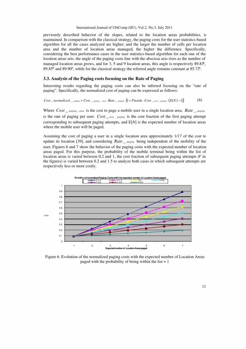
Interesting results regarding the paging costs can also be inferred focusing on the “rate of paging”. Specifically, the normalized cost of paging can be expressed as follows:
( )[ ]1][_1____ __ −⋅⋅+⋅⋅= N E Cost Pinside RateCost normalized Cost pagingnext pagingarea paging paging (6)
Where area pagingCost __ is the cost to page a mobile user in a single location area, paging Rate _
is the rate of paging per user, pagingnext Cost __ is the cost fraction of the first paging attempt
corresponding to subsequent paging attempts, and E[ N ] is the expected number of location areaswhere the mobile user will be paged.
Assuming the cost of paging a user in a single location area approximately 1/17 of the cost toupdate its location [39], and considering paging Rate _ being independent of the mobility of theuser, Figures 6 and 7 show the behavior of the paging costs with the expected number of locationareas paged. For this purpose, the probability of the mobile terminal being within the list of location areas is varied between 0.2 and 1, the cost fraction of subsequent paging attempts (F inthe figures) is varied between 0.2 and 1.5 to analyze both cases in which subsequent attempts arerespectively less or more costly.
0
0.1
0.2
0.3
0.4
0.5
0.6
0.7
0.8
0.9
1
1 2 3 4 5 6 7Expected number of Location Areas paged
Evolutio n of normalized Paging Costs with the expected number of Location Areas pagedF=1.5 F=1.2 F=1 F=0.8F=0.6 F=0.4 F=0.2
Figure 6. Evolution of the normalized paging costs with the expected number of Location Areas
paged with the probability of being within the list = 1
Costs
8/6/2019 Savings in Location Management Costs Leveraging User Statistics
http://slidepdf.com/reader/full/savings-in-location-management-costs-leveraging-user-statistics 13/20
International Journal of UbiComp (IJU), Vol.2, No.3, July 2011
13
0
0.05
0.1
0.15
0.2
0.25
0.3
1 2 3 4 5 6 7
Expected number of Location Areas paged
Evolution of normalized Paging C osts with the expected number of Location Areas paged
F=1.5 F=1.2 F=1 F=0.8
F=0.6 F=0.4 F=0.2
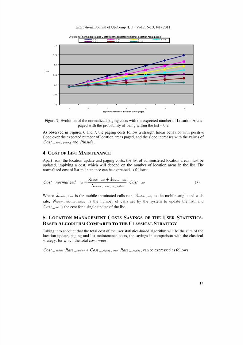
Figure 7. Evolution of the normalized paging costs with the expected number of Location Areaspaged with the probability of being within the list = 0.2
As observed in Figures 6 and 7, the paging costs follow a straight linear behavior with positiveslope over the expected number of location areas paged, and the slope increases with the values of
pagingnext Cost __ and Pinside .
4. COST OF LIST MAINTENANCE
Apart from the location update and paging costs, the list of administered location areas must beupdated, implying a cost, which will depend on the number of location areas in the list. Thenormalized cost of list maintenance can be expressed as follows:
list
updatetocallsumber
origmobiletermmobilelist Cost
N normalized Cost ___
___
__
⋅+= λ λ (7)
Where termmobile _λ is the mobile terminated calls rate, origmobile _λ is the mobile originated callsrate, updatetocallsumber N ___ is the number of calls set by the system to update the list, and
list Cost _ is the cost for a single update of the list.
5. LOCATION MANAGEMENT COSTS SAVINGS OF THE USER STATISTICS-
BASED ALGORITHM COMPARED TO THE CLASSICAL STRATEGY
Taking into account that the total cost of the user statistics-based algorithm will be the sum of thelocation update, paging and list maintenance costs, the savings in comparison with the classical
strategy, for which the total costs were
updateupdate RateCost __ ⋅ + pagingarea paging RateCost __ _ ⋅ , can be expressed as follows:
Costs
8/6/2019 Savings in Location Management Costs Leveraging User Statistics
http://slidepdf.com/reader/full/savings-in-location-management-costs-leveraging-user-statistics 14/20
International Journal of UbiComp (IJU), Vol.2, No.3, July 2011
14
list
updatetocallsumber
origmobiletermmobile
pagingnext pagingarea paging
updateupdate
Cost N
N E Cost RateCost
N RateCost PinsideSavings
_
1][___
11__
___
__
__ )](
[
⋅+
−−⋅⋅
−
−⋅⋅=
⋅
⋅
λ λ
(8)
By means of (8), the performance of the user statistics-based algorithm can be evaluated in boththe radio interface and the fixed network parts.
5.1. Location Management costs savings in the radio interface
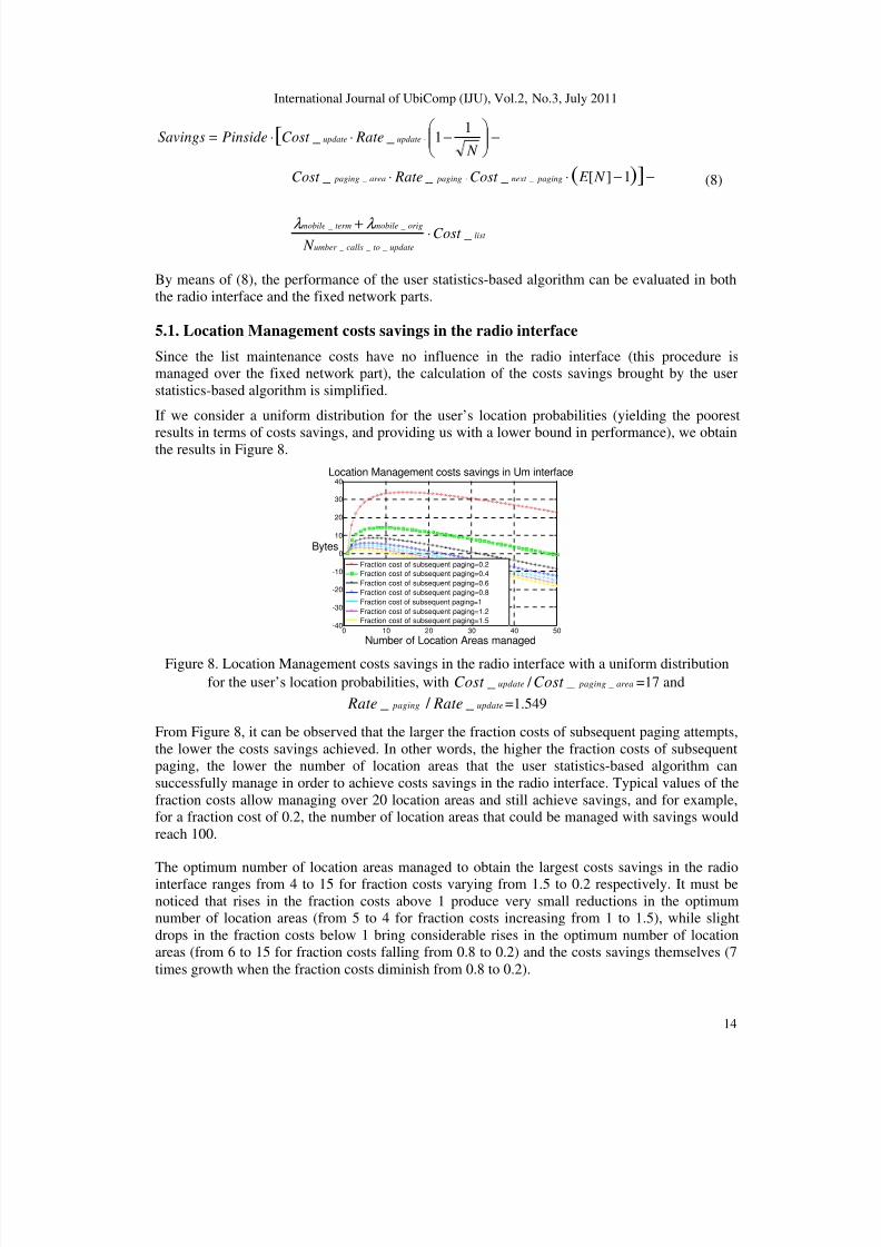
Since the list maintenance costs have no influence in the radio interface (this procedure ismanaged over the fixed network part), the calculation of the costs savings brought by the userstatistics-based algorithm is simplified.
If we consider a uniform distribution for the user’s location probabilities (yielding the poorest
results in terms of costs savings, and providing us with a lower bound in performance), we obtainthe results in Figure 8.
0 10 20 30 40 50-40
-30
-20
-10
0
10
20
30
40
Number of Location Areas managed
Bytes
Location Management costs savings in Um interface
Fraction cost of subsequent paging=0.2
Fraction cost of subsequent paging=0.4
Fraction cost of subsequent paging=0.6
Fraction cost of subsequent paging=0.8
Fraction cost of subsequent paging=1
Fraction cost of subsequent paging=1.2
Fraction cost of subsequent paging=1.5
Figure 8. Location Management costs savings in the radio interface with a uniform distributionfor the user’s location probabilities, with updateCost _ / area pagingCost __ =17 and
paging Rate _ update Rate _ / =1.549
From Figure 8, it can be observed that the larger the fraction costs of subsequent paging attempts,the lower the costs savings achieved. In other words, the higher the fraction costs of subsequentpaging, the lower the number of location areas that the user statistics-based algorithm cansuccessfully manage in order to achieve costs savings in the radio interface. Typical values of thefraction costs allow managing over 20 location areas and still achieve savings, and for example,for a fraction cost of 0.2, the number of location areas that could be managed with savings wouldreach 100.
The optimum number of location areas managed to obtain the largest costs savings in the radiointerface ranges from 4 to 15 for fraction costs varying from 1.5 to 0.2 respectively. It must benoticed that rises in the fraction costs above 1 produce very small reductions in the optimumnumber of location areas (from 5 to 4 for fraction costs increasing from 1 to 1.5), while slightdrops in the fraction costs below 1 bring considerable rises in the optimum number of locationareas (from 6 to 15 for fraction costs falling from 0.8 to 0.2) and the costs savings themselves (7times growth when the fraction costs diminish from 0.8 to 0.2).
8/6/2019 Savings in Location Management Costs Leveraging User Statistics
http://slidepdf.com/reader/full/savings-in-location-management-costs-leveraging-user-statistics 15/20
International Journal of UbiComp (IJU), Vol.2, No.3, July 2011
15
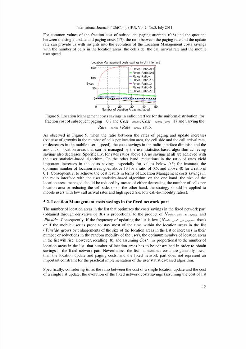
For common values of the fraction cost of subsequent paging attempts (0.8) and the quotientbetween the single update and paging costs (17), the ratio between the paging rate and the updaterate can provide us with insights into the evolution of the Location Management costs savingswith the number of cells in the location areas, the cell side, the call arrival rate and the mobileuser speed.
0 10 20 30 40 50
0
50
100
150
Number of Location Areas managed
Bytes
Location Management costs savings in Um interface
Rates Ratio=0.1
Rates Ratio=0.5Rates Ratio=1
Rates Ratio=1.5
Rates Ratio=2Rates Ratio=5
Rates Ratio=10
Figure 9. Location Management costs savings in radio interface for the uniform distribution, for
fraction cost of subsequent paging = 0.8 and updateCost _ / area pagingCost __ =17 and varying the paging Rate _ update Rate _ / ratio.
As observed in Figure 9, when the ratio between the rates of paging and update increases(because of growths in the number of cells per location area, the cell side and the call arrival rate,or decreases in the mobile user’s speed), the costs savings in the radio interface diminish and theamount of location areas that can be managed by the user statistics-based algorithm achievingsavings also decreases. Specifically, for rates ratios above 10, no savings at all are achieved withthe user statistics-based algorithm. On the other hand, reductions in the ratio of rates yieldimportant increases in the costs savings, especially for values below 0.5; for instance, theoptimum number of location areas goes above 13 for a ratio of 0.5, and above 40 for a ratio of 0.1. Consequently, to achieve the best results in terms of Location Management costs savings inthe radio interface with the user statistics-based algorithm, on the one hand, the size of the
location areas managed should be reduced by means of either decreasing the number of cells perlocation area or reducing the cell side, or on the other hand, the strategy should be applied tomobile users with low call arrival rates and high speed (i.e. low call-to-mobility ratios).
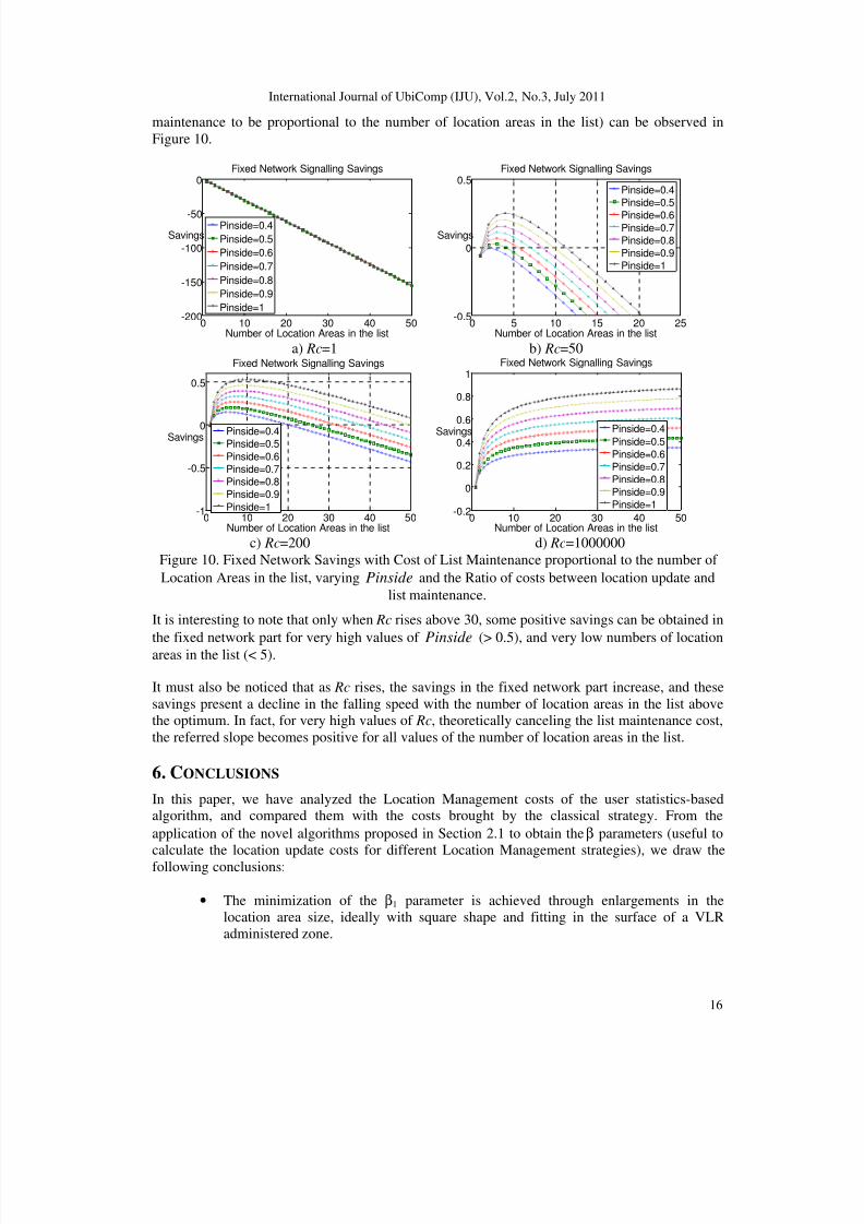
5.2. Location Management costs savings in the fixed network part
The number of location areas in the list that optimizes the costs savings in the fixed network part(obtained through derivative of (8)) is proportional to the product of updatetocallsumber N ___ andPinside . Consequently, if the frequency of updating the list is low ( updatetocallsumber N ___ rises)or if the mobile user is prone to stay most of the time within the location areas in the list( Pinside grows by enlargements of the size of the location areas in the list or increases in theirnumber or reductions in the random mobility of the user), the optimum number of location areasin the list will rise. However, recalling (8), and assuming list Cost _ proportional to the number of
location areas in the list, that number of location areas has to be constrained in order to obtainsavings in the fixed network part. Nevertheless, the list maintenance costs are generally lowerthan the location update and paging costs, and the fixed network part does not represent animportant constraint for the practical implementation of the user statistics-based algorithm.
Specifically, considering Rc as the ratio between the cost of a single location update and the costof a single list update, the evolution of the fixed network costs savings (assuming the cost of list
8/6/2019 Savings in Location Management Costs Leveraging User Statistics
http://slidepdf.com/reader/full/savings-in-location-management-costs-leveraging-user-statistics 16/20
International Journal of UbiComp (IJU), Vol.2, No.3, July 2011
16
maintenance to be proportional to the number of location areas in the list) can be observed inFigure 10.
0 10 20 30 40 50-200
-150
-100
-50
0
Number of Location Areas in the list
Savings
Fixed Network Signalling Savings
Pinside=0.4
Pinside=0.5
Pinside=0.6
Pinside=0.7
Pinside=0.8
Pinside=0.9
Pinside=1
0 5 10 15 20 25-0.5
0
0.5
Number of Location Areas in the list
Savings
Fixed Network Signalling Savings
Pinside=0.4Pinside=0.5
Pinside=0.6Pinside=0.7Pinside=0.8Pinside=0.9Pinside=1
a) Rc=1 b) Rc=50
0 10 20 30 40 50-1
-0.5
0
0.5
Number of Location Areas in the list
Savings
Fixed Network Signalling Savings
Pinside=0.4Pinside=0.5
Pinside=0.6Pinside=0.7Pinside=0.8Pinside=0.9
Pinside=10 10 20 30 40 50
-0.2
0
0.2
0.4
0.6
0.8
1
Number of Location Areas in the list
Savings
Fixed Network Signalling Savings
Pinside=0.4Pinside=0.5Pinside=0.6Pinside=0.7Pinside=0.8Pinside=0.9Pinside=1
c) Rc=200 d) Rc=1000000
Figure 10. Fixed Network Savings with Cost of List Maintenance proportional to the number of Location Areas in the list, varying Pinside and the Ratio of costs between location update and
list maintenance.
It is interesting to note that only when Rc rises above 30, some positive savings can be obtained in
the fixed network part for very high values of Pinside (> 0.5), and very low numbers of locationareas in the list (< 5).
It must also be noticed that as Rc rises, the savings in the fixed network part increase, and thesesavings present a decline in the falling speed with the number of location areas in the list abovethe optimum. In fact, for very high values of Rc, theoretically canceling the list maintenance cost,the referred slope becomes positive for all values of the number of location areas in the list.
6. CONCLUSIONS
In this paper, we have analyzed the Location Management costs of the user statistics-basedalgorithm, and compared them with the costs brought by the classical strategy. From theapplication of the novel algorithms proposed in Section 2.1 to obtain the β parameters (useful tocalculate the location update costs for different Location Management strategies), we draw thefollowing conclusions:
• The minimization of the β1 parameter is achieved through enlargements in thelocation area size, ideally with square shape and fitting in the surface of a VLRadministered zone.
8/6/2019 Savings in Location Management Costs Leveraging User Statistics
http://slidepdf.com/reader/full/savings-in-location-management-costs-leveraging-user-statistics 17/20
International Journal of UbiComp (IJU), Vol.2, No.3, July 2011
17
• The minimization of the β21 and β22 parameters requires reductions in the size of thelocation areas and rises in the number of cells within the VLR administered zone,whose shape should be as regular as possible.
From the analysis of the location update costs for the user statistics-based algorithm, we can inferthe following guidelines:
• Increases in the VLR administered zone size (keeping the number of cells per locationarea fixed) bring declines in the location update costs and rises in their decreasing speedwith the number of cells per location area.
• Hexagonal cells schemes deliver lower location update costs and higher decreasingspeeds in those costs than the square ones, although the difference is reduced as thenumber of cells per location area grows.
• The larger the summation of the probabilities controlled by the user statistics-basedalgorithm, the lower the location update costs, regardless of the actual number of thoselocation areas.
Regarding the paging costs in the user statistics-based algorithm, we can observe the followingtrends:
• The paging costs decline as the summation of the probabilities of the location areasadministered by the user statistics-based algorithm grows.
• The slope of the paging costs grows with the value of the fraction costs for subsequentpaging attempts ( pagingnext Cost __ ) and the probability of the user being within the
location areas in the list ( Pinside ).
In connection with the Location Management costs savings of the user statistics-based algorithmfor the radio interface, we can highlight the following interesting points:
• The optimum number of location areas to keep in the list ranges from 4 to 15 for valuesof pagingnext Cost __ varying from 1.5 to 0.2 respectively.
• Increases in pagingnext Cost __ above unity produce very small declines in the optimum
number of location areas (e.g. from 5 to 4 as pagingnext Cost __ grows from 1 to 1.5),
while reductions in pagingnext Cost __ under 1 deliver noticeable rises in the optimum
number of location areas (e.g. from 6 to 15 when pagingnext Cost __ drops from 0.8 to 0.2)
and the costs savings themselves (e.g. 7 times growth as pagingnext Cost __ falls from 0.8to 0.2).
• The performance of the user statistics-based algorithm in comparison with the classicalstrategy improves as the users’ call-to-mobility ratios drop (preferably below 0.5).
And for the Location Management costs savings in the fixed network part, assuming the cost of asingle update of the list ( list Cost _ ) to be proportional to the number of location areas in the list,we can draw the following conclusions:
8/6/2019 Savings in Location Management Costs Leveraging User Statistics
http://slidepdf.com/reader/full/savings-in-location-management-costs-leveraging-user-statistics 18/20
International Journal of UbiComp (IJU), Vol.2, No.3, July 2011
18
• For values of the ratio between the costs of a single location update and a single listupdate ( Rc) underneath 30, no savings are obtained in the fixed network part, and thelarger the number of location areas administered, the larger the losses.
• For a particular value of Rc, the lower Pinside , the bigger the losses or the smaller the
savings, depending on the particular value of Rc.• The optimum number of location areas in the list rises with Pinside , and this growth is
emphasized with increases in Rc.
• For the highest achievable values of Rc (over 50), the optimum number of location areasin the list to obtain savings in the fixed network part ranges between 3 and 10, dependingon Pinside (preferably above 0.4).
In conclusion, the user statistics-based algorithm outperforms the classical strategy, especially forthe highest values (> 0.5) of the mobility predictability level of the location areas most frequentlyvisited by the user. And in order to optimize its performance, the most favorable number of location areas to maintain in the list would range from 4 to 8, keeping the number of cells per
location area for densely populated areas below 15.
REFERENCES
[1] Vijayakumar, H.; Ravichandran, M.; “Efficient location management of mobile node in wirelessmobile ad-hoc network”, Proceedings of National Conference on Innovations in EmergingTechnology, NCOIET'11, p 77-84, 2011
[2] E. Martin, R. Bajcsy, “Variability of Location Management Costs with Different Mobilities andTimer Periods to Update Locations”, International Journal of Computer Networks &Communications, 2011.
[3] E. Martin; “Characterization of the Costs provided by the Timer-based method in LocationManagement”, 7th International Conference on Wireless Communications, Networking andMobile Computing, 2011.
[4] E. Martin; “A graphical Study of the Timer Based Method for Location Management with theBlocking Probability”, 7th International Conference on Wireless Communications, Networkingand Mobile Computing, 2011.
[5] E. Martin, and R. Bajcsy; “Enhancements in Multimode Localization Accuracy Brought by aSmart Phone-Embedded Magnetometer”, IEEE International Conference on Signal ProcessingSystems, 2011.
[6] Almeida-Luz, Sónia M.; Vega-Rodríguez, Miguel A.; Gómez-Púlido, Juan A.; Sánchez-Pérez,Juan M.; “Differential evolution for solving the mobile location management”, Applied SoftComputing Journal, v 11, n 1, p 410-427, January 2011
[7] Gállego, José Ramón; Canales, María; Hernández-Solana, Ángela; Valdovinos, Antonio;“Adaptive paging schemes for group calls in mobile broadband cellular systems”, IEEEInternational Symposium on Personal, Indoor and Mobile Radio Communications, PIMRC, p
2444-2449, 2010[8] Lee, Jong-Hyouk; Pack, Sangheon; You, Ilsun; Chung, Tai-Myoung; “Enabling a paging
mechanism in network-based localized mobility management networks”, Journal of InternetTechnology, v 10, n 5, p 463-472, 2009
[9] Goel, Ashish; Gupta, Navankur; Kumar, Prakhar; “A speed based adaptive algorithm for reducingpaging cost in cellular networks”, Proceedings - 2009 2nd IEEE International Conference onComputer Science and Information Technology, ICCSIT 2009, p 22-25, 2009.
8/6/2019 Savings in Location Management Costs Leveraging User Statistics
http://slidepdf.com/reader/full/savings-in-location-management-costs-leveraging-user-statistics 19/20
International Journal of UbiComp (IJU), Vol.2, No.3, July 2011
19
[10] E. Martin; “Multimode radio fingerprinting for localization”, IEEE Radio and Wireless Week,IEEE Topical Conference on Wireless Sensors and Sensor Networks, Phoenix, Arizona, January2011, pp. 383-386.
[11] Martin, E.; Lin, G.; Weber, Matt; Pesti, Peter; Woodward, M.; “Unified analytical models forlocation management costs and optimum design of location areas”, 5th International Conferenceon Collaborative Computing: Networking, Applications and Worksharing, CollaborateCom, 2009,pp. 1-10.
[12] Toril, Matías; Luna-Ramírez, Salvador; Wille, Volker; Skehill, Ronan; “Analysis of user mobilitystatistics for cellular network re-structuring”, IEEE 69th Vehicular Technology Conference, VTCSpring 2009, pp. 1-9.
[13] Tabbane, S., “An alternative strategy for location tracking” IEEE Journal on Selected Areas inCommunications, v.13, n.5, pp. 880-892, 1995.
[14] Tabbane, S., “Comparison between the alternative location strategy (AS) and the classical locationstrategy (CS)” WINLAB, Rutgers Univ., Piscataway, NJ, Technical Report 37, Sept. 1992.
[15] E. Martin, and T. Lin, “Probabilistic Radio Fingerprinting Leveraging SQLite in Smart Phones”,IEEE International Conference on Signal Processing Systems, 2011.
[16] Amar Pratap Singh, J.; “Intelligent location management using soft computing technique”, 2nd
International Conference on Communication Software and Networks, pp. 343-346, 2010.[17] E. Martin, and R. Bajcsy, “Analysis of the Effect of Cognitive Load on Gait with off-the-shelf
Accelerometers”, Cognitive 2011, Rome, Italy.
[18] E. Martin et al., “Enhancing Context Awareness with Activity Recognition and RadioFingerprinting”, International Conference Semantic Computing, 2011.
[19] E. Martin; “Solving training issues in the application of the wavelet transform to precisely analyzehuman body acceleration signals”, Proceedings of the 2010 IEEE International Conference onBioinformatics and Biomedicine, 2010, pp. 427-432.
[20] Xiao, Y., “Optimal location management for two-tier PCS networks”, Computer Communications,v 26, n 10, pp. 1047-1055, 2003.
[21] E. Martin; “Real time patient’s gait monitoring through wireless accelerometers with the wavelettransform”, IEEE Radio and Wireless Week, IEEE Topical Conference on Biomedical WirelessTechnologies, Networks, and Sensing Systems, Phoenix, Arizona, January 2011, pp. 23-26.
[22] E. Martin; “Novel method for stride length estimation with body area network accelerometers”,IEEE Radio and Wireless Week, IEEE Topical Conference on Biomedical Wireless Technologies,Networks, and Sensing Systems, Phoenix, Arizona, January 2011, pp. 79-82.
[23] E. Martin; “Optimized Gait Analysis Leveraging Wavelet Transform Coefficients from BodyAcceleration”, 2011 International Conference on Bioinformatics and Biomedical Technology,March 2011.
[24] E. Martin, and R. Bajcsy; “Considerations on Time Window Length for the Application of theWavelet Transform to Analyze Human Body Accelerations”, International Conference SignalProcessing Systems, 2011.
[25] E. Martin et al., “Linking Computer Vision with off-the-shelf Accelerometry through KineticEnergy for Precise Localization”, International Conference Semantic Computing, 2011.
[26] E. Martin, V. Shia, R. Bajcsy; “Determination of a Patient’s Speed and Stride Length MinimizingHardware Requirements”, Body Sensor Networks, May 2011.
[27] CCIR “Future public land mobile telecommunications systems” Doc. 8/1014-E, December 1989.
[28] Yuen, W., Wong, W., “Dynamic location area assignment algorithm for mobile cellular systems”,IEEE International Conference on Communications, v 3, pp. 1385-1389, 1998.
8/6/2019 Savings in Location Management Costs Leveraging User Statistics
http://slidepdf.com/reader/full/savings-in-location-management-costs-leveraging-user-statistics 20/20
International Journal of UbiComp (IJU), Vol.2, No.3, July 2011
20
[29] Lei, Z., Rose, C., “Probability criterion based location tracking approach for mobility managementof personal communications systems”, Conference Record / IEEE Global TelecommunicationsConference, v 2, p 977-981, 1997.
[30] Chang, R., Chen, K., “Dynamic mobility tracking for wireless personal communication networks”,Annual International Conference on Universal Personal Communications - Record, 1997, v 2, pp.448-452, 1997.
[31] Watanabe, Y., Yabusaki, M., “Mobility/traffic adaptive location management”, IEEE VehicularTechnology Conference, v 56, n 2, pp. 1011-1015, 2002.
[32] Cao, P., Wang, X., Huang, Z., “Dynamic location management scheme based on movement-state”,Acta Electronica Sinica, v 30, n 7, p 1038-1040, 2002.
[33] Tabbane, S., “Location management methods for third-generation mobile systems”, IEEECommunications Magazine, pp. 72-84, August 1997.
[34] D. MacFarlane and S. Griffin, “The MPLA Vision of UMTS”, CODIT/BT/PM-005/1.0, Feb.1994.
[35] Seskar, I., Maric, S., “Rate of location area updates in cellular systems” Proceedings IEEEVehicular Technology Conference 92, May 1992, Denver, CO.
[36] Meier-Hellstern, K. S., “The use of SS7 and GSM to support high density personalcommunications” Proceedings IEEE ICC’92, June 1992, Chicago, IL, paper 356.2.
[37] Kourtis, S.; Tafazolli, R., “Modelling cell residence time of mobile terminals in cellular radiosystems”, Electronics Letters, Jan 2002, v 38, n 1, p. 52-54.
[38] Tabbane, S., “An alternative strategy for location tracking” IEEE Journal on Selected Areas inCommunications, 1995, v.13, n.5, p. 880-892.
[39] Thomas, R., Gilbert, H., and Mazziotto, G., “Influence of the moving of the mobile stations on theperformance of a radio mobile cellular network”, Proceedings 3rd Nordic Seminar, Sept. 1988,Copenhagen, Denmark, paper 9.4.
Authors
E. Martin is carrying out research in the Department of Electrical Engineering and Computer Science atUniversity of California, Berkeley. He holds a MS in Telecommunications Engineering from Spain and aPhD from England within the field of location management for mobile telecommunications networks. Hehas research experience in both industry and academia across Europe and USA, focusing on wirelesscommunications, sensor networks, signal processing and localization.
R. Bajcsy received the Master’s and Ph.D. degrees in electrical engineering from the Slovak Republic, andthe Ph.D. in computer science from Stanford University, California. She is a Professor of ElectricalEngineering and Computer Sciences at the University of California, Berkeley. Prior to joining Berkeley,she headed the Computer and Information Science and Engineering Directorate at the National ScienceFoundation. Dr. Bajcsy is a member of the National Academy of Engineering and the National Academy of Science Institute of Medicine as well as a Fellow of the Association for Computing Machinery (ACM) andthe American Association for Artificial Intelligence. In 2001, she received the ACM/Association for theAdvancement of Artificial Intelligence Allen Newell Award, and was named as one of the 50 mostimportant women in science in the November 2002 issue of Discover Magazine.


![RetainingWomen [Read-Only] · SAVINGS FACULTY RETENTION Estimated savings associated with retaining a faculty member in one STEM field: $383,000 Costs of replacement: $78,516 Costs](https://static.fdocuments.us/doc/165x107/5f56cca92aaa8d233631db6f/retainingwomen-read-only-savings-faculty-retention-estimated-savings-associated.jpg)