
Savings and Tax Incentives: Semiparametric Estimation of the
32
Savings and Tax Incentives: Semiparametric Estimation of the Household Savings Impact of RRSPs. Kevin S. Milligan * Department of Economics, University of Toronto May, 1998 - This revision: July 1998 Abstract Tax incentives to encourage saving constitute an increasingly important component of gov- ernment pension policy worldwide. Empirical evidence of their ability to raise household savings levels, however, is conflicting. This paper employs a semiparametric estimator to explore this problem through the study of the RRSP program in Canada. Several interesting results emerge. First, RRSP savings are found to partially, yet not fully, crowd out savings in other forms. Sec- ond, comparing different methods of controlling for observable characteristics reveals insights about the magnitude of selection bias. Third, little evidence of substitution between RRSPs and illiquid forms of savings is found. * The author thanks, but does not implicate, Rajeev Dehejia, Keith Horner, Jack Mintz, Abigail Payne, Michael Smart, and Jeffrey Smith for helpful comments and assistance. The support of the Social Sciences and Humanities Research Council is acknowledged. 1
Transcript of Savings and Tax Incentives: Semiparametric Estimation of the

Savings and Tax Incentives: Semiparametric Estimation of theHousehold Savings Impact of RRSPs.
Kevin S. Milligan∗
Department of Economics, University of Toronto
May, 1998 - This revision: July 1998
Abstract
Tax incentives to encourage saving constitute an increasingly important component of gov-ernment pension policy worldwide. Empirical evidence of their ability to raise household savingslevels, however, is conflicting. This paper employs a semiparametric estimator to explore thisproblem through the study of the RRSP program in Canada. Several interesting results emerge.First, RRSP savings are found to partially, yet not fully, crowd out savings in other forms. Sec-ond, comparing different methods of controlling for observable characteristics reveals insightsabout the magnitude of selection bias. Third, little evidence of substitution between RRSPsand illiquid forms of savings is found.
∗The author thanks, but does not implicate, Rajeev Dehejia, Keith Horner, Jack Mintz, Abigail Payne, MichaelSmart, and Jeffrey Smith for helpful comments and assistance. The support of the Social Sciences and HumanitiesResearch Council is acknowledged.
1

1 Introduction
In response to demographic, economic, and political pressures, governments worldwide have been
moving away from large public pension plans in the direction of systems based on individual saving.
This movement has been explicit in some countries, while in others it has occurred more quietly
through the atrophy of public programs. Common to many countries is an increasing reliance on
tax assisted savings programs as a central feature of government pension policy. Strikingly, the
effectiveness of such programs in raising household savings remains unclear. Simple theory suggests
an ambiguous effect on household savings, while empirical evidence has been indecisive. This paper
will take a fresh empirical approach to this question in hope of providing new insight.
Tax deferred savings plans are the most common type of tax assistance for savings. Typically,
investments placed within the plan, as well as income from those investments, are not subject to
taxation until withdrawal. This allows savings to accumulate at the tax-free rate of interest, as
well as deferring taxes on the principal. The Individual Retirement Account (IRA) and 401(k)
programs in the United States, and the Registered Retirement Savings Plan (RRSP) program in
Canada, are representative examples.
Most analysis of tax assisted savings is firmly rooted in a life cycle savings paradigm. In this
framework, a change in the after tax return to saving is a change in the relative price of future to
current consumption. As with any change in relative prices, the increase in the return to saving
leads to a substitution and an income effect. The lower relative price of future consumption induces
substitution from current to future consumption,1 which increases current savings. However, the
increase in the return to saving will cause net savers to feel wealthier. This increases current
consumption and decreases savings, so long as consumption is a normal good. These competing
income and substitution effects imply that the overall effect on savings should be ambiguous.2
As well, empirical evidence regarding the interest elasticity of consumption suggests that house-
holds do not have strong savings responses to changes in interest rates. (See, for example, Hall1Ragan (1994) develops a model that delivers a substitution effect toward current consumption in the presence of
a progressive income tax.2If there is a statutory limit to contributions, then households desiring to save more than the limit will have only
an income effect, since the change in the return to savings is inframarginal. In this case, the predicted effect onsavings is unambiguously negative.
2

1988 or Campbell and Mankiw 1989.) This invites skepticism to the suggestion that households
make large adjustments to levels of savings in response to a change in the rate of return.
The source of the empirical difficulty in estimating the savings impact of tax deferred savings
programs is a missing data problem. Because the econometrician cannot observe what contributing
households would have saved in the absence of the program, the missing data must be inferred from
elsewhere. Most have approached this problem by making inferences from the savings behaviour
of noncontributing households. Such inferences become appreciably more difficult if the two sets
of households differ in the relevant characteristics that determine savings behaviour. Different
strategies to account for this heterogeneity underlie the disparate empirical findings.
Venti and Wise (1986, 1990) developed a formal model to describe savings behaviour in the pres-
ence of IRAs, finding that up to 65 cents of each dollar saved within the program represented net
new savings. Their method was criticised in Gale and Scholz (1994) for, among other things, impos-
ing identical coefficients and error structures on both contributing and noncontributing households.
With an alternative model, they found that IRAs were close substitutes for other forms of savings,
implying that IRAs created an insignificant amount of new net savings. Poterba, Venti, and Wise
(1996) responded by highlighting the sensitivity of the Gale and Scholz method to the definitions
of types of savers. Using a slightly modified version of the Gale and Scholz specification, they find
the model can deliver a prediction of substantial net new savings. This empirical imbroglio failed
to produce a clear consensus.
More recently, a number of authors have taken to the problem with approaches requiring fewer
parametric assumptions. Venti and Wise (1995, 1996) have turned to the use of a cohort estimation
method. By comparing the asset holdings of households reaching a given age in different years, a
difference in difference estimator is suggested. The household reaching the given age in the later
year has had a longer period of exposure to the program. This difference in exposure is assumed
to be a source of exogenous variation that generated the observed changes in assets. Engelhardt
(1996) makes use of a more lucid natural experiment by examining the cancellation of the RHOSP3
program in Canada, looking at differences between contributing and noncontributing households
before and after its cancellation. These papers find little evidence of crowding out other forms of
savings. Venti and Wise (1995, p. 1) conclude that “in virtually no instance do the micro data3The Registered Home Ownership Savings Plan (RHOSP) provided tax exempt savings for qualifying households.
It was cancelled in 1986.
3
show substitution between RRSP and other forms of personal saving.”
Nevertheless, methodological problems linger. Not enough care is taken to account for differ-
ences in savings behaviour caused by observable differences between contributing and noncontribut-
ing households. Some inferences are made on the basis of unconditional means, while others rely
on methods imposing identical coefficients and error structures on all observations. In addition,
savings behaviour is estimated during the turbulent macroeconomic era of the late 1970s to mid
1980s, which imperils inferences predicated on a stable experimental environment.
The present paper will take a new approach in the hope of addressing some of these criticisms.
Bernheim (1997) describes an ideal experiment in which eligible households are randomly assigned
to one of two groups: one group is permitted to contribute to the savings program, while the other
group is not. This creates exogenous variation in eligibility that could be exploited to measure
the savings impact of the program. Recent work in the program evaluation literature (Heckman,
Ichimura, and Todd 1997; Heckman, Ichimura, Smith and Todd 1998; Dehejia and Wahba 1998;
Angrist 1998) has advanced the use of nonexperimental estimators to replicate the results of exactly
the type of fictitious social experiment described by Bernheim.
Viewing the measurement of savings program effects as a program evaluation problem, this
paper will adopt a nonexperimental estimator to examine the differences in savings behaviour
of contributors and noncontributors to the RRSP program in Canada. By comparing different
methods of controlling for observable characteristics, the evidence suggests that unobservable char-
acteristics may not have strong influence on the results. As well, the estimator facilitates the
analysis of different measures of savings, allowing for some inferences about substitutability among
different classes of assets. Finally, the estimates of the net new savings created by participation in
the RRSP program suggest that previous estimates have been overstated.
2 Empirical method
Fully randomized experiments have many desirable properties.4 If households could be assigned
in some random way to participate in a savings incentive program, then the distribution of house-
hold characteristics relevant to the savings decision, both observable and unobservable, would be
identical for contributing and noncontributing households. Without access to such an experiment,4Heckman and Smith (1995) provide a comprehensive comparison of experimental and nonexperimental estimation.
4
however, nonexperimental estimators can provide results with similar properties to those from a
fully controlled random experiment. This section will describe an estimator that matches obser-
vations with similar observable characteristics in order to obtain a measurement of the effect of
participation on household saving.
2.1 Matching on the Propensity Score
Matching facilitates comparisons between like contributing and noncontributing households, with-
out forcing strong assumptions on parameters. Gale and Scholz (1994, p. 1250) justify the exclusion
of households with extreme levels of savings from their data set with allusion to evidence that there
may be “different saving responses to observed characteristics among the wealthy.” This argument
captures a certain wariness concerning parametric assumptions about households with dissimilar
observables. The matching estimator described below takes their argument to heart by ensuring
that inferences are made only from households with similar characteristics.
The notation used here is adapted from that appearing in Heckman et al. (1997). Each house-
hold has a desired level of savings for each of two possible mutually exclusive contingencies. In
states in which it chooses to contribute, the household saves Scon. In states in which it does not
contribute, the household saves Snon. Of course, only one of these will be revealed in the data.
The household is assigned C = 1 if it contributes and C = 0 if it does not. The relevant observ-
able characteristics for the household’s savings decision are contained in X. The propensity score
p(X) represents the probability a household will participate in the program, given its observable
characteristics, or
p(X) ≡ prob(C = 1 | X) . (1)
Rosenbaum and Rubin (1983) show that, under certain conditions, controlling for observables
using p(X) is sufficient. This means that conditioning on one-dimensional p(X) is equivalent to
conditioning on multi-dimensional X. This dimensional reduction substantially eases the burden of
conditioning on observable characteristics. A more detailed discussion of this estimator is provided
in Appendix A.
We want to know what contributing households would have saved if there had been no program.
In other words, the parameter of interest is the impact of participation on the participants. Given
5
a propensity score, the net savings impact of contributing to the program is defined in this way:
δ[p(X)] ≡ E[Scon − Snon | p(X), C = 1] (2)
Moving the expectations operator through the bracket yields
δ[p(X)] = E[Scon | p(X), C = 1]− E[Snon | p(X), C = 1]. (3)
The first term in the right hand side of (3) is observable. The second term represents what a
household that did contribute would have saved had there been no program. This is counterfactual,
so it must be inferred from another source. The obvious candidate for this job is the savings of
noncontributors, E[Snon | p(X), C = 0].
Making this substitution, the calculation that will be made from the data is
δ[p(X)] = E[Scon | p(X), C = 1]− E[Snon | p(X), C = 0]. (4)
Under the conditions outlined in Appendix A, δ[p(X)] will identify the amount of created savings
δ[p(X)]. This measurement will be well defined only over regions where the support of p(X) for
contributors overlaps with that for noncontributors. Let S represent this common support set. If
the parameter of interest is redefined to be the average effect of contributions on savings only in S,
then it can be calculated as
δS = ES{δ[p(X)]} =∫
Sδ[p(X)]× df [p(X) | p(X) ∈ S]. (5)
Concern over this redefinition of the parameter of interest should be inversely related to the
proportion of the support of (p(X) | C = 1) contained in S.
This estimator is similar in spirit to the two step estimator of Heckman (1979), with two
important differences. First, matching on the propensity score controls for observables in a non-
linear way. Second, it relaxes the assumption of a constant, additively separable treatment effect.
6

As with the traditional two step estimator, confidence in the procedure depends on developing a
good model of selection.
2.2 Implementation
In order to apply this empirical strategy, a method of conditioning on the propensity score must
be chosen. Heckman et al. (1997) and Dehejia and Wahba (1998) outline a variety of possibilities.
The two methods described below each have both benefits and drawbacks.
2.2.1 Stratified Matching
Rosenbaum and Rubin (1984) suggest a method in which observations are sorted into strata based
on their propensity scores. The aim is to find a set of strata that allows plausible inferences from
noncontributors to contributors. In a balanced stratification, the means of the explanatory variables
in each stratum are not significantly different for contributors and noncontributors. Dehejia and
Wahba (1998) provide an algorithm to guide this otherwise ad hoc process. This method can be
useful when there are large differences in the density of p(X) for contributors and noncontributors
for some intervals in S .
Once a balanced stratification is found, the mean difference in the savings of noncontributors
and contributors is calculated for each stratum. A weighted average of these differences is found,
using the number of contributors in each stratum as weights.
2.2.2 Direct Matching
A second approach matches each contributing household with a similar noncontributing household.
The difference in savings of the two households is found, and the mean of these differences across
all matched pairs is calculated to obtain δS . Direct matching works well if there is a large number
of noncontributing households at all intervals in S . If this is not the case, problems can ensue.
Using matching with replacement, the unique best match for each contributing household is
found. If a particular noncontributing household is the best match for many contributing house-
holds, that household may carry undue weight in the calculation of δS . On the other hand, if obser-
vations are discarded after having been matched, there can occur a shortage of suitable matches in
some intervals in S . If the shortage of noncontributing households in some intervals in S becomes
acute, the quality of the matches will deteriorate.
7

2.3 Comparison with Linear Estimators
In order to highlight the difference between this empirical approach and more traditional specifi-
cations, some simple OLS models will be estimated. These estimators will take the form
Si = β′Zi + αCi + εi, (6)
where Ci is the contribution status of household i, Zi is a vector of covariates, and εi is an error
term, with a normal (0, σε2) distribution. Zi will contain combinations of the household’s observable
characteristics and a polynomial in the propensity score.
The assumptions embodied in this specification can be placed in two groups. First, this spec-
ification assumes that participation is uncorrelated with unobservables; that there is no selection
bias. Second, the functional form of the model is assumed to be linear with constant parameters,
with the same distribution of errors for all observations. If these assumptions hold, then estimating
α from this equation may identify the effect of contribution on savings.
The analysis of the linear models has two goals. First, by progressively adding polynomial
terms in p(X) of higher degree, some intermediate steps linking the simple linear estimator to the
matching estimator will be filled in. This will help indicate the way in which p(X) controls for
observables. Second, examination of the intermediate steps may reveal insights about the relative
importance of violations of the selection bias and functional form assumptions.
3 Empirical Test
3.1 Dataset Description
This empirical strategy will be applied to participants in the RRSP program in Canada for the years
1986, 1990, and 1992. Contributions to RRSPs, and interest income from previously contributed
investments, are not subject to taxation until withdrawal. The RRSP program began in 1957, with
increasingly widespread participation and promotion since the expansion of the program in the mid
1970s. Any tax filer under the age of 71 was eligible to contribute up to 18% (20% before 1991) of
earned income each year, up to a limit.5 Contributions in taxation year 1992 were made by 24.9%
of tax filers, with an average contribution of $3057 (Canada 1994). The trends in participation,
contribution limits, and levels of contribution are presented in Figure (1).5Since 1991, those making contributions to eligible private pension plans have an adjustment made to their limit.
8

The RRSP program is an attractive case to consider for two reasons. First, because of its
relatively long history, it can be thought of as a mature program. This contrasts with studies
of IRAs that were constrained by the need to account for the diffusion of information about the
program through the years under study. Second, the breadth and depth of the available data allows
for the generation of desired explanatory variables.
Data was taken from the Survey of Family Expenditures (FAMEX) for each of the years under
consideration. The FAMEX is a questionnaire based survey which asks selected households from
each of the ten provinces to recall expenditures and transactions from the past calendar year.
Follow-up interviews are conducted, and responses checked for consistency. The means of the
variables used in this analysis for each of the three years are presented in Table I. The 1990
survey restricted the sample to include only households from 15 metropolitan areas, and so was
correspondingly smaller than the other two years under consideration. In both 1990 and 1986, the
household’s province of residence was not available. Instead, the region of residence was reported.
Some observations had to be excluded from consideration. First, households in which the
reference person6 was 71 or older were discarded, as they were ineligible for participation. As well,
a handful of observations with null responses in key variables were not kept.
3.2 Definition of Savings
An attractive feature of this estimation method is the ability to compare different measures of
saving. Once households have been matched, any available definitions of savings may be compared
with ease. This is exploited here through the use of three measures, with the hope of observing the
sensitivity of the results to the definition of savings. All three of these definitions measure the flow
of savings during a given year, rather than looking at the stock of savings at a particular point in
time.
3.2.1 broad
The first measure of savings, labelled broad, includes the change in total household assets less
liabilities during the year. For financial assets, only net purchases less sales is included, which
disregards unrealised capital gains. Looking at the financial tx variable in Table I, contributors are
roughly twice as likely as noncontributors to have made a transaction involving financial assets. If6The FAMEX defines the person who is “mainly responsible for the financial maintenance of the household” as
the reference person.
9

this ratio is also indicative of the holdings of financial assets by contributors and noncontributors,
then this exclusion of capital gains from consideration will systematically underestimate the increase
in savings of contributors.
Broad does include changes in housing equity, which is contentious. Bernheim (1997) discusses
evidence showing that households tend to think of housing equity as a very special form of sav-
ings, for which little substitution is likely. Gale (1997) enumerates several reasons why broader
asset definitions deliver more compelling results, with reference to evidence that broader measures
show more substitution. Separate from that debate, Canadian households might be more likely to
substitute housing equity for other forms of savings, since mortgage interest is not deductible in
Canada (Carroll and Summers 1987). Engelhardt (1996) used this same measure for his analysis
of the RHOSP program.
3.2.2 y-c
The second measure, y-c, subtracts household expenditures from income. It was used by Venti and
Wise (1995), who note that the probable understatement of expenditures in household surveys like
the FAMEX will cause this measure to overestimate savings.7 This also a broader measure, but
includes no unrealised gains or losses on assets held. Importantly, it does not include changes in
housing equity.
3.2.3 liquid
The third measure, liquid, focuses on the net change in liquid assets. The use of narrower measures
is justified if only liquid financial assets are displaced by contributions to a retirement savings plan.
Similar measures were used by Venti and Wise (1990, 1995, 1996). Engen, Gale, and Scholz (1996)
criticised this measure for failing to include changes in household debt. As well, households making
purchases or sales of large assets (such as houses or cars) may exhibit precipitous fluctuations in
this measure, since they are substituting to forms of savings not captured by liquid.
3.3 Model of Participation
A model of RRSP participation is needed to obtain the propensity score for each household. RRSP
participation was previously modelled by Venti and Wise (1988), while Engelhardt (1996) pre-7Since a difference between contributors and noncontributors will be taken, this potential overstatement is only
of concern to the extent that it varies systematically between contributors and noncontributors.
10

sented a similar model of RHOSP participation. Participation in 401(k) plans was studied in
Bassett, Fleming, and Rodrigues (1998). Using these models as a point of departure, a comparable
parsimonious model of participation is estimated. Following that, an extended set of explanatory
variables is introduced to enhance the predictive power of the model by using all available and
relevant observable characteristics.
There are two explanatory variables which may fail to be exogenous. First, because a contri-
bution to an RRSP might change a household’s marginal effective tax rate (METR), the METR
could be endogenous. This problem is resolved by using the METR facing the household for its
first dollar of contribution. The second potentially problematic variable is the household’s income.
Deaton (1987) scolds those using contemporaneous income instead of a measure of permanent in-
come for the estimation of savings behaviour. In spite of this, the use of current income continued
unabated in the literature. To confront this concern, some simple overidentification tests8 were per-
formed to gauge the importance of measuring the income variable with error. These tests showed
no significant impact on the estimates.
3.3.1 Simple Model
Following the program evaluation literature, a logit specification was estimated. The maximum
likelihood estimates appear as model (i) in Table II. Appendix B contains a description of each
explanatory variable, and Appendix C contains an overview of the construction of a household’s
METR.
For most variables, the signs and relative magnitudes of the coefficients are consistent with
previous findings. The estimated coefficients for the METR are 1.54, 1.39, and 3.14 for 1992, 1990,
and 1986 respectively. These are similar in magnitude to those from previous studies. The estimates
in Engelhardt (1996) however, were much less precise. The source of this difference is likely found
in the generation of the METR variable. By taking more care to account for clawbacks, deductions
and credits, the METR used here contains more information. The METR in Engelhardt (1996)
amounted to little more than a transformation of income through the tax tables. Bassett, Fleming,
and Rodrigues (1998) do not include the METR in their model of participation.
The estimated METR coefficient for 1986 is nearly twice the magnitude of the coefficient for8The number of bathrooms and the number of rooms in the dwelling served as instruments indicative of a house-
hold’s permanent income.
11

1990 and 1992. This may be caused by the differences in the tax structure resulting from the
Canadian tax reform of 1988.9 Since the number of tax brackets were reduced, it may have become
less likely that contributing could jump a household to a lower tax bracket. A contribution would
still lower the household’s total tax bill, but the importance of the marginal tax rate would be
diminished with fewer brackets.
The coefficients on married, income, age, and professional were all positive and strongly signif-
icant. This is consistent with expectations based on life cycle behaviour. Looking at the education
indicators, having a university degree does not make contribution more likely, but completing high
school and some post-secondary education do.
Those participating in private pension plans were more likely to contribute to an RRSP.10 This
result is counterintuitive, as future pension benefits ought to crowd out the need for current RRSP
saving. However, this apparent anomaly has occurred regularly in past studies.
3.3.2 Extended Model
The variables contained in the extended set of regressors can be placed in four classes. First, a
number of variables are introduced to capture a household’s taste for savings. These include an
indicator for making a purchase or sale of a financial asset, as well as a variable to measure the
proportion of a household’s income coming from investment income. Second, a number of sup-
plementary demographic variables will augment those found in model (i). These include variables
indicating the characteristics of the spouse and children in the household. Next, geographic indica-
tors may pick up taxation or fixed behavioural differences among residents of different provinces,
and between rural and urban dwellers. Finally, some interaction and polynomial terms were added
to ease the process of stratifying the observations. The maximum likelihood estimates are presented
as model (ii) in Table II.
Importantly, most of the coefficients on the variables intended to capture a household’s taste
for saving are significant. Financial tx had a very strong effect on participation, as did housing
equity. Investment income was significant only for 1986. This is crucial because the participation
model must minimize the impact of any unobservable characteristics that may be correlated with9The tax reform of 1988 replaced many deductions (that reduced taxable income) with tax credits (that reduce
tax payable), as well as decreasing the number of tax brackets from 10 to 3. RRSP contributions continued to betreated as a deduction from taxable income after the reform.
10Only a household’s employee contributions were available. This neglects households that are beneficiaries ofnoncontributory pension plans.
12

the participation decision. These strong, significant coefficients build confidence in the ability of
the model to account for a household’s taste for savings.
The addition of the extended set of variables affected the estimated coefficients from model (i)
in different ways for different variables. The estimated coefficient for other pension lost both size
and significance, falling from 0.24 to 0.11 in 1992, for example. This may have been due to the
inclusion of other variables reflecting a household’s taste for savings. The coefficient on METR
retained its magnitude and significance for all years. For the spouse of the reference person, age
and professional have the strongest influence. Finally, living in a large urban centre or in a rural
area does not seem to be an important factor for RRSP participation.
3.4 Digression: Assessing the Use of this Estimator for Savings Program Eval-uation.
Matching on the propensity score has not been used previously to evaluate savings programs. In
order to assess its applicability to this question, the comprehensive analysis of its use in evaluating
the JTPA11 found in Heckman et al. (1997, 1998) will be used as a benchmark. First, the model
of program participation is appraised, followed by a discussion of the ‘support problem.’
Heckman et al. (1997, p. 633) conclude that “matching on P (X) works well if it is based
on a good model of program participation.” The JTPA analysis benefits from a wealth of earlier
work on JTPA participation. For the RRSP program, fewer precedents are available. On the
other hand, JTPA participation analysis has been constrained by a lack of consistently available
explanatory variables. The model of RRSP participation presented here enjoys the luxury of a rich
set of explanatory variables, including some strong indicators of a household’s taste for savings.
This RRSP participation model is unlikely to be insuperable, but it does seem sufficient compared
with others used to generate propensity scores in other contexts.
The matching estimator defined in (5) can be interpreted only over the region of common
support S. If S excludes much of the support of contributing households, then the interpretation
of δS loses vigour. This ‘support problem’ manifested itself in the JTPA analysis presented in
Heckman et al. (1998), as the region of common support was limited to the interval [0, 0.225].
In contrast, the comparison of the histograms of the propensity scores for RRSP participation
presented in Figure (2) shows the extent of the region of overlapping support. In practice, no more11The Job Training Partnership Act (JTPA) is a job training program in the United States.
13
than a handful of contributors were excluded from S for any of the estimations presented here.
Any optimism must be tempered by the state of relative ignorance regarding the structure
of unobserved savings heterogeneity. There is no obvious relationship between the structure of
heterogeneity for labour market characteristics and that for savings characteristics. This limits the
inferences that can be made from the evaluation of matching in other contexts. Still, the relative
strength of the model of participation and the absence of a support problem provide some degree
of confidence.
4 Results
Table III displays the estimated impact of participation on household savings for contributing
households. Results are reported for five estimation methods using three measures of savings for
each year. The first column is included to show the importance of conditioning on observables.
It contains the unconditional mean difference of contributors and noncontributors. The second
and third columns display the results using stratified matching on the propensity score. The
regression adjusted results were obtained by estimating a simple OLS equation for each stratum
of noncontributors. These estimated coefficients were applied to the corresponding contributor
observations to obtain the reported regression adjusted savings estimates. The fourth and fifth
columns contain the results from direct pairwise matching on the propensity score, with and without
replacement. Since the best match for each contributor observation is not unique when matching
without replacement, the contributors were randomly ordered before matching occurred.
The average change in contributors’ savings must be adjusted for the impact on net savings of the
tax reduction received when contributing.12 Because the tax reduction will reduce public savings,
the standard approach is to subtract the tax reduction from the change in private savings to find
the overall change in net savings. Recognising that a contribution creates a future tax liability for
the household can lead to virtually the same calculation, although with a different interpretation.
If savings is defined as the change in household wealth, the future tax liability generated by a
contribution must be taken into consideration. With this interpretation, subtracting the present
value of future taxes from the change in savings to find the net savings impact is equally appropriate.
To the extent that households may face a lower tax rate upon retirement,13 the present value of12The tax reduction was calculated using the simple average of the MTR before and after the RRSP contribution.13In Canada, Old Age Security payments are clawed back at the rate of for those with family incomes exceeding
14

the future tax liability may be exceeded by the current tax savings. However, the effect of this on
current consumption behaviour is unlikely to be large.14
The tax reduction received when contributing is subtracted from the estimated difference in
savings in order to arrive at an estimate of net new savings. This is divided by the average
RRSP contribution to find the percentage of RRSP contributions that represents net new savings.
Displaced savings constitutes the percentage of the RRSP contribution that crowded out other
forms of savings. It is calculated as the remainder of the RRSP contribution unaccounted for by
the tax reduction or new savings.
For example, In Table III the 1992 regression adjusted estimate of the difference in savings
between contributors and noncontributors for the broad measure is $1535. The average tax reduction
received by contributors for their contribution was $993, leaving $542 as the estimate of net new
savings. The average contribution of $2615 can then be broken down into a tax reduction of $993
(38%) and net new savings of $542 (20.7%), with the remaining $1080 (41.3%) coming from other
forms of savings.
Using means to describe the effect of participation leaves the results susceptible to influential
outliers. To examine the sensitivity of the results to influential outliers, the models were estimated
using a data set excluding extreme15 savers. The excluded observations represented approximately
one percent of the total number of observations. There was no significant difference in the results
compared to the full data set.
4.1 How much of RRSP contributions represent new savings?
The results from the matching estimation show evidence of RRSPs crowding out other forms of
savings. The unconditional differences in the first column are obviously much larger than can
be explained by RRSP contributions, as the estimates generally show that more than 100% of
contributions represent new savings. However, by controlling for observable characteristics, the
next four columns of Table III do uncover evidence that some of the funds placed in RRSPs
displace savings in other forms. A summary of the results appears below in Table IV.
$53 215. The proposed Seniors’ Benefit has similar provisions, with a lower threshold for the clawback. This meansthat it is plausible that the tax smoothing motive for contributing may be diminished, or even reversed for manycontributing households.
14If the household’s behaviour is Ricardian, then this difference will have no effect on consumption.15Households saving more than 75,000 or dissaving more than 50,000 were excluded.
15
Table IV - Summary of ResultsYear Unadj. Strat. Adj. Strat. Matching with Repl. Matching without Repl.1992 50.3 20.7 41.1 39.01990 73.1 47.0 18.5 78.61986 52.2 45.4 52.9 35.7
cells indicate percentage of RRSP contribution that represents new saving.
The results range from 18.5% to 78.6%. The smaller sample size of the 1990 data set may have
contributed to the more extreme variation in results for that year. Looking only at the years with
the larger data set, the range of the estimates becomes 20.7% to 52.9%.
This evidence suggests partial, but not complete crowding out of other forms of savings by
RRSP contributions. Some, but certainly not all, of RRSP contributions do represent net new
savings. The claim of Venti and Wise (1995) that the micro data does not show substitution in
any instance appears to be false. At the same time, the assumption of complete crowding out
underlying Ragan’s (1996) call for the curtailment of the RRSP program must be reconsidered.
4.2 Linking Linear Models to Matching
In order to better understand the advantages of matching estimation over more traditional meth-
ods, the OLS models described in section 2.3 were estimated, with the results appearing in Table
V. These results are also useful to check some of the assumptions made to justify the matching
estimators. To focus the comparison, only the broad measure of savings is used. Regressions using
the other measures showed similar results.
To begin, comparing the results of models (i) and (ii) provides a check on the performance of
p(X) as a proxy for X. The propensity score appears to deliver comparable estimates to condition-
ing on X, although with slightly less precision. For example, the 1986 estimates of new savings are
29.4% and 27.8%, for conditioning on X and p(X) respectively. Since these are not significantly
different from each other, this provides grounds to have confidence in the index sufficiency condition
underlying matching on p(X).
Looking at model (i), the estimates of the impact of participation are conspicuously smaller
than the estimates obtained from matching. If unobservable characteristics are correlated with the
contribution decision, then estimates of the savings impact of participation α will overestimate any
constant linear treatment effect. However, the OLS estimate of α of 29.4% is smaller than matching
16
estimates of 35.7% to 52.9%. This is equally true for 1990 and 1992.
Since the removal of selection bias would lead to smaller estimates, the presence of larger es-
timates by matching suggests that it is the functional form assumptions that drive the disparity
between OLS and matching estimates. This could mean one of two things. First, it may be the case
that matching estimates make no improvement on simple linear models in controlling for selection
bias. On the other hand, a more encouraging interpretation is the possibility that the observable
characteristics employed here successfully capture the important elements of the participation de-
cision, leaving unobservables with little explanatory power. In this case, this evidence provides
confidence in the assumptions underlying matching on p(X).
The importance of allowing for more general functional forms can be seen clearly in Table
V. As more complicated polynomial terms in p(X) are added in models (iii), (iv) and (v), the
estimated difference in savings draws nearer to the matching estimates found in Table III. Inspecting
the results for 1986, the estimated net new savings is 35.8% when conditioning on a fifth degree
polynomial in p(X), while the corresponding matching estimates in Table III range from 35.7%
to 52.9%. As conditioning on observable variables takes place in more complicated and less linear
ways, the OLS estimates approach the matching estimates.
4.3 Comparing Measures of Savings
If some classes of assets are imperfect substitutes for others, changes in the value of a particular
class of assets may not lead to rebalancing of portfolios or changes in consumption-saving decisions.
For example, if housing equity is not a substitute for other forms of saving, then an appreciation
in the price of houses would not be reflected in liquid, but would be included in broad.16 Of course,
stickiness in portfolio transactions may fade over longer time periods, so inferences about asset
substitution made from examining savings over this 12 month period are limited. To guide the
interpretation of asset substitution for the years in question, the rates of return for several relevant
classes of assets are provided in Table VI.
Comparing the performance of different measures of savings in Table III, no clear patterns are
evident. For 1986 and 1990, the estimated net new savings using liquid is not noticeably different
than with the broader measures. This is contrary to the prediction of Gale (1997) that broader16The FAMEX reports the value of the household’s dwelling at December 31 of the year in question. In such a
survey, the accuracy of the response may be called into question
17

measures should show more substitution. If liquid shows the same degree of substitution as broader
measures, this would legitimize the use of narrower definitions of savings. In 1992, however, liquid
shows systematically less substitution than the other two measures. This may be explained by
the introduction in 1992 of a tax exemption on funds removed from RRSPs for the purpose of
purchasing a home. Any such substitution of housing equity for RRSP savings would affect broad
but not liquid. This would lead to greater observed substitution for broader measures of savings.
5 Conclusions
This paper has considered the study of RRSP savings as a program evaluation problem, delivering
several interesting results. First, the results indicate that some of each dollar contributed to the
RRSP program represents net new saving. Second, a comparison of the results of simple OLS
regressions and those from matching estimations may suggest that selection bias does not have
strong influence on the estimates of savings behaviour, given a reasonably rich set of observables.
Third, little evidence is found that broader measures show more substitution between RRSPs and
other household assets, at least over a one year period.
If, for example, only 40 cents of each dollar is new savings, then is the program worthwhile?
Hubbard and Skinner (1996) present simulation evidence indicating that new savings at this level
may be sufficient for the program to be self financing. Their computations are set in the framework
of Feldstein (1995), which relies on a country’s success in capturing the full return to new investment.
The new investment would spur higher corporate and personal tax revenues, eventually overtaking
the negative revenue impact of tax reductions for savings plan contributions. In an open economy
like Canada, complete domestic capture of the full return to investment is less likely to hold.
However, it may be the case that the levels of new savings found here are high enough to make the
program self financing.
Intractable measurement problems afflict empirical examination of savings. Classes of savings
differ in rates of return, tax treatment, and risk, meaning that a dollar of savings in one form may
not represent the same amount of expected future consumption as a dollar in another form.17 This
suggests that interpretations of aggregated savings be made with caution. Furthermore, explicit or17Intertemporal asset pricing models suggest that marginal reallocations of assets within a portfolio should leave
expected future consumption unchanged. However, these marginal conditions do not imply that the total amount ofsavings in different forms will provide the same future consumption.
18

implicit promises by government or family members to provide future consumption may represent
a substantial proportion of a household’s ‘savings’, defined very broadly. Changes in these forms
of savings that vary systematically across contributors and noncontributors may be important in
determining the level of observable savings, as well as the degree of substitution among observable
classes of assets. The intangible nature of these forms of savings makes their measurement very
difficult.
Notwithstanding these problems, the evidence presented here confirms that tax incentives to
encourage saving can be an effective policy tool. Even so, this empirical result lacks a convincing
theoretical context into which it may be placed. This constrains predictions about the effects of
marginal shifts of policy parameters. There remain many significant questions in the investigation
of this critical area of public policy.
19

A Appendix - Discussion of Matching on p(X)
This appendix describes in more detail the matching estimator used in this paper. If it is assumed
that selection into the program can be explained by observable characteristics, then the distribution
of savings will be independent (⊥) of contributor status, given the observable characteristics.
Scon, Snon⊥C | X (A-1)
This assumption may be cause for legitimate concern. If a household’s decision to participate
in the program is dependent on an unobservable taste for saving, then (A-1) will be violated. Of
course, completely controlling for covariates that are unobservable is a fundamentally insurmount-
able challenge without access to a randomized experiment. Accepting this, the problem becomes
one of choosing an estimator with the best properties for this task, relative to other potential
estimators.
A primary benefit of the semiparametric approach is that conditioning need not eliminate bias,
merely balance the bias across participants and nonparticipants (Heckman 1996 and Heckman and
Smith 1996). This is in contrast to the standard assumptions requiring that the expected value of
the error for both participants and nonparticipants be equal to zero in order to identify treatment
effects. The semiparametric assumption is weaker.
Rosenbaum and Rubin (1983) show that (A-1), along with the assumption that
0 < p(X) < 1, (A-2)
implies that conditioning on p(X) is sufficient. This means that given a propensity score, the
distribution of savings for contributors and noncontributors will be the same:
Scon, Snon⊥C | p(X). (A-3)
20

Heckman and Smith (1996) stress that assumption (A-3) is stronger than is necessary to justify
standard matching estimators. Since inferences will be made only from the observed behaviour of
noncontributors, it is necessary only to assume that the distribution of savings in noncontributing
states will be independent of contributor status, given the observable characteristics. This means
the following weaker assumption (A-3a) will suffice:
Snon⊥C | p(X). (A-3a)
This resembles the outcome of an experimental study in the sense that the distribution of
X for contributors and noncontributors with similar propensity scores is the same. This would
be equivalent to a randomized experiment in which the randomizing takes place with respect to
observables only. The assumptions in (A-3a) allow the identification of the net savings impact of
program participation.
If (A-3) holds, then expected savings in non-contributing states is independent of contributor
status given p(X), or
E[Snon | p(X), C = 1] = E[Snon | p(X), C = 0] = E[Snon | p(X)]. (7)
This means that, given (A-1) and (A-2), measuring δ[p(X)] as in (4) will identify the treatment
effect δ[p(X)] defined in (2).
Along with the relaxation of restrictions on parameters, the other key difference between match-
ing and regression estimators for program evaluation is the weight given to observations in calculat-
ing the treatment effect (Angrist 1998). Matching estimators weight the treatment effect at a given
level of X proportional to the probability of participation at that level of X. Regression estimators
weight proportional to the variance of participation at a particular level of X. This distinction
grows in importance as the probability of participation among participants grows.
B Marginal Tax Rate Calculations.
In order to model the participation decision, the marginal tax rate facing the household on its
first dollar of RRSP contribution must be approximated. The marginal tax rate (MTR) for the
21

individual in the household with the highest earnings was taken to be the MTR facing the household.
Because of the tax reform of 1988, the approach taken to estimating the MTR for 1992 and 1990
differed from that for 1986.
B.1 1992, 1990
In the federal tax reform of 1988, most deductions from taxable income were changed to credits
against taxes payable. So, for the purposes of this calculation, taxable income for most households
was taken to be earned income. The taxable income of the reference person was assigned one of
the three federal tax brackets (fedmtr). Next, federal tax credits were subtracted from federal tax
payable to determine if the threshold for federal surtax (fedsur) was reached. For each individual,
the basic personal amount, age amount, married amount, CPP/QPP contributions, UIC contribu-
tions, allowable transfers from the spouse, and child tax credit were calculated from the available
data. The average of credits not included in this calculation amounted to only a few hundred
dollars. Tax credits only affect MTRs to the extent that they determine on which side of the surtax
threshold the individual falls, as well as whether the MTR is zero. So, the number of cases where
this approximation will be in error, and the size of the error in those cases, is likely to be small.
The amount of some federal tax credits declines with income. The child tax credit, and the
Goods and Services Tax credit both begin to be ‘clawed back’ at a 5% rate when family income
reaches a certain threshold. Family allowance and Old Age Security are clawed back at a 15% rate
on the individual’s income. The inclusion of the total of these clawbacks (claw) can substantially
increase the marginal tax rate facing a household.
Provincial income taxes are levied as a percentage of federal tax payable, at a rate (provrate)
that varies across provinces. Some provinces also apply a surtax (provsur) on tax payable over a
certain threshold, and others apply a flat surtax (provflat) on taxable income. For 1990, the province
of residence is not available, so the provincial rate was calculated using a weighted average of the
provinces included in the region, with the number of tax filers in each province used as weights.
Combining all this information yields the following calculation for the marginal tax rate facing
the household on its first dollar of RRSP contribution:
MTR = fedmtr × (1 + provrate× (1 + provsur) + fedsur) + provflat + claw
22

Quebec is an exception. Federal tax is calculated in the same way, but with a 16.5% tax
abatement on federal tax payable. Provincial tax is calculated on a base of taxable income which
differs slightly from the federal taxable income base. It has a progressive structure, with 5 tax
brackets. The provincial marginal tax rate was added to the standard federal marginal tax rate to
obtain an approximation of the overall marginal tax rate facing a household from Quebec.
B.2 1986
Before the 1988 tax reform, individuals had access to many more deductions from earned income,
but faced a rate structure that had 10 brackets and somewhat higher rates. Provincial income
taxes in 1986 took the same structure as in 1992, but fewer provinces had surtaxes and the rates
were generally lower.
The deductions used to calculate the reference person’s taxable income were the basic personal
exemption, age exemption, married exemption, dependent children exemption, CPP/QPP contri-
butions, UIC contributions, interest and dividend income deduction, union and professional dues,
employment expense deduction, and eligible transfers from spouse. From this point, the calculation
proceeds in the same way as for 1992, although with different rates and thresholds.
C Variable Descriptions
broad - net change in household assets and liabilitiesy-c - household income less total household expenditureliquid - cash held in banks, etc. , financial assets (net purchases less sales), RRSP (net contributionsless withdrawals)RRSP - net contributions less withdrawalsincome - total household income before taxesMETR - first dollar marginal effective tax rate for reference personother pension - dummy variable indicating contribution to other (non-RRSP, non-CPP/QPP) pen-sion planhousing equity - value of dwelling owned by household on December 31 less principal owing onmortgageinvestment income - proportion of income derived from investmentsfinancial tx - dummy variable indicating household had non-zero level of net purchases less sales offinancial assetschildren - number of children in the household
reference person:married - dummy variable indicating whether reference person is marriedage - age of reference personmale - dummy variable indicating if reference person is malefarm/fish - dummy variable indicating reference person is employed as a farmer or a fisherman
23

professional - dummy variable indicating reference person is employed in Managerial and Admin-istrative, Professional and Technical, or Teaching fieldshigh school - dummy variable indicating reference person completed high schoolpost-secondary - dummy variable indicating reference person had some post-secondary educationuniversity - dummy variable indicating reference person has university degree
spouse:age to university - variables same as for reference personemployed - dummy variable indicating spouse had earned incomerural - dummy variable indicating household located in rural areabig urban centre - dummy variable indicating household located in city of 100,000 or moreAtlantic - dummy variable indicating household located in Newfoundland, New Brunswick, NovaScotia, or PEIPrairie - dummy variable indicating household located in Manitoba or Saskatchewan
D References
Angrist, Joshua D. (1998), “Estimating the Labor Market Impact of Voluntary Military ServiceUsing Social Security Data on Military Applicants,” Econometrica, Vol. 66, pp. 249-288.
Basset, William F., Michael J. Fleming, and Anthony P. Rodrigues (1998), “How Workers Use401(k) Plans: The Participation, Contribution, and Withdrawal Decisions,” National Tax Journal,Vol. 51 pp.
Bernheim, Douglas B. (1997), “Rethinking Saving Incentives,” in Alan J. Auerbach (ed.) FiscalPolicy: Lessons from Economic Research,” Cambridge, Mass.: MIT Press.
Campbell, John Y. and N. Gregory Mankiw (1989), “Consumption, Income, and Interest Rates:Reinterpreting the Time Series Evidence,” in NBER Macroeconomics Annual, Cambridge, Mass.:MIT Press.
Canada (1984-1994), Tax Statistics on Individuals, Revenue Canada.
Carroll, Chris and Lawrence H. Summers (1987), “Why Have Private Savings Rates in the UnitedStates and Canada Diverged?” Journal of Monetary Economics, Vol. 20, pp. 249-279.
Deaton, Angus (1987), “Comment - IRAs and Savings” in Martin S. Feldstein (ed.) The Effects ofTaxation on Capital Accumulation, Chicago, Ill.: The University of Chicago Press.
Dehejia, Rajeev H. and Sadek Wahba (1998), “Causal Effects in Non-Experimental Studies: Re-evaluating the Evaluation of Training Programs,” NBER Working Paper 6586.
Engen, Eric M, William G. Gale, and John Karl Scholz (1996), “The Illusory Effects of SavingsIncentives on Saving,” Journal of Economic Perspectives, Vol. 10, pp. 113-138.
Engelhardt, Gary V. (1996),“Tax Subsidies and Household Saving: Evidence from Canada,” Quar-terly Journal of Economics, Vol. 111, pp. 1237-1268.
24

Feldstein, Martin (1995), “The Effects of Tax-Based Saving Incentives on Government Revenueand National Saving,” Quarterly Journal of Economics, Vol. 110, pp. 475-494.
Gale, William G. (1997), “Comment - Rethinking Savings Incentives,” in Alan J. Auerbach (ed.)Fiscal Policy: Lessons from Economic Research,” Cambridge, Mass.: MIT Press.
Gale, William G. and John Karl Scholz (1994), “IRAs and Household Saving,” American EconomicReview, Vol. 84, pp. 1233-1260.
Hall, Robert E. (1988), “Intertemporal Substitution in Consumption,” Journal of Political Econ-omy, Vol. 96, pp. 339-357.
Heckman, James J. (1979), “Sample Selection Bias as a Specification Error.” Econometrica, Vol.47, pp. 153-161.
Heckman, James J. (1996), “Randomization as an Instrumental Variable,” Review of Economicsand Statistics, Vol. 56, pp. 336-341.
Heckman, James J., Hidehiko Ichimura, Jeffrey Smith, and Petra Todd (1998), “CharacterizingSelection Bias Using Experimental Data,” forthcoming in Econometrica.
Heckman, James J., Hidehiko Ichimura, and Petra E. Todd (1997), “Matching as an EconometricEvaluation Estimator: Evidence from Evaluating a Job Training Programme,” Review of EconomicStudies, Vol. 64, pp. 605-654.
Heckman, James J. and Jeffrey A. Smith (1995), “Assessing the Case for Social Experiments,”Journal of Economic Perspectives, Vol. 9, pp. 85-110.
Heckman, James J. and Jeffrey A. Smith (1996), “Experimental and Nonexperimental Evaluation”in Gunther Schmid, Jacqueline O’Reilly and Klaus Schomann (eds.) International Handbook ofLabour Market Policy and Evaluation Cheltenham, U.K.: Edward Elgar.
Hubbard, Glenn R. and Jonathan S. Skinner (1996), “Assessing the Effectiveness of Saving Incen-tives,” Journal of Economic Perspectives, Vol. 10, pp. 73-90.
Poterba, James M., Steven F. Venti, and David A. Wise (1996), “How Retirement Saving ProgramsIncrease Saving,” Journal of Economic Perspectives, Vol. 10, pp. 91-112.
Ragan, Christopher (1994), “Progressive Income Taxes and the Substitution Effect of RRSPs,”Canadian Journal of Economics, Vol. 27, pp. 43-57.
Ragan, Christopher (1996), ”A Case for Abolishing Tax-Deferred Savings Plans, ”in J. Richardsand William G. Watson (eds.) When We’re 65, Toronto: C.D. Howe Institute, pp. 57-92.
Rosenbaum, Paul R. and Donald B. Rubin (1983), “The Central Role of the Propensity Score inObservational Studies for Causal Effects,” Biometrika, Vol. 70, pp. 41-55.
25

Rosenbaum, Paul R. and Donald B. Rubin (1984), “Reducing Bias in Observational Studies UsingSubclassification on the Propensity Score,” Journal of the American Statistical Association, Vol.79, pp. 516-524.
Venti, Steven F. and David A. Wise (1986), “Tax-Deferred Accounts, Constrained Choice, andEstimation of Individual Saving,” Review of Economic Studies, Vol. 53, pp. 579-601.
Venti, Steven F. and David A. Wise (1988), “The Determinants of IRA Contributions and theEffect of Limit Changes,” in Zvi Bodie, John B. Shoven, and David A. Wise (eds.) Pensions in theU.S. Economy, Chicago, Ill.: The University of Chicago Press.
Venti, Steven F. and David A. Wise (1990), “Have IRAs Increased U.S. Saving?: Evidence fromConsumer Expenditure Surveys,” Quarterly Journal of Economics, Vol. 105, pp. 661-698.
Venti, Steven F. and David A. Wise (1995), “RRSPs and Saving in Canada,” Mimeo.
Venti, Steven F. and David A. Wise (1996), “The Wealth of Cohorts: Retirement Saving and theChanging Assets of Older Americans,” NBER Working Paper 5609.
26
Table I
Unconditional Means of Contributors and Noncontributors
1992 1990 1986all cons. noncons. all cons. noncons. all cons. noncons.
observations 8153 3081 5072 4039 1489 2550 9123 2550 6573broad 1835 5023 -102 2608 5995 630 1273 4669 -45y-c 1761 5046 -234 2474 5842 508 1168 4596 -162liquid 1096 3549 -394 1341 3472 97 798 3150 -114RRSP 991 2622 0 949 2575 0 624 2233 0income 48238 65187 37943 49811 63668 41720 37259 51736 31643METR(%) 32.0 37.7 28.5 32.9 37.2 30.3 28.9 36.7 25.8other pension(%) 17.7 25.3 13.1 19.0 24.4 15.8 16.8 24.8 13.7housing equity 58518 84845 42526 63110 87207 49039 41753 65254 32636investment inc.(%) 3.2 3.7 2.9 3.3 3.9 3.0 4.2 5.6 3.6financial tx(%) 23.4 36.4 15.4 29.0 40.7 22.2 28.3 44.4 22.0children 0.77 0.78 0.76 0.78 0.70 0.83 0.81 0.71 0.85reference person:married(%) 65.8 76.3 59.4 65.5 72.7 61.3 67.2 76.3 63.6age 43.7 44.2 43.4 42.7 44.1 41.9 42.9 44.9 42.1male(%) 58.7 64.3 55.4 58.3 62.3 56.0 71.6 78.2 69.1farm/fish(%) 2.8 2.3 3.1 0.9 1.3 0.7 3.3 2.2 3.7professional(%) 26.0 38.2 18.6 31.1 42.4 24.6 25.3 39.4 19.9high school(%) 87.3 93.5 83.5 90.5 94.0 88.5 83.7 90.8 81.0post-secondary(%) 44.7 58.2 36.5 49.7 59.4 44.1 38.8 52.8 33.3university(%) 14.5 22.5 9.7 16.3 22.8 12.5 12.8 22.2 9.2spouse:age 42.6 43.4 42.1 41.3 42.9 40.3 42.7 43.6 42.3farm/fish(%) 2.1 1.5 2.5 0.7 0.8 0.7 0.8 0.9 0.7professional(%) 78.3 64.2 86.8 79.2 72.9 82.8 74.7 56.5 81.8high school(%) 88.0 93.5 84.6 92.1 95.4 90.2 93.7 91.4 94.7post-secondary(%) 42.2 53.5 35.4 46.8 56.1 41.3 47.4 44.2 48.6university(%) 12.0 18.1 8.2 13.8 19.0 10.7 14.2 13.4 14.5employed(%) 66.7 73.8 62.5 69.9 74.4 67.3 58.0 63.4 55.9rural(%) 13.7 9.8 16.1 ** ** ** 11.7 8.5 12.9big urban centre(%) 63.5 69.5 59.9 100.0 100.0 100.0 64.9 70.4 62.7Atlantic(%) ** ** ** 17.5 14.6 19.2 19.5 15.2 21.2Newfoundland(%) 5.8 4.2 6.8 ** ** ** ** ** **P.E.I.(%) 3.2 3.2 3.3 ** ** ** ** ** **Nova Scotia(%) 6.3 5.0 7.1 ** ** ** ** ** **New Brunswick(%) 6.9 6.3 7.3 ** ** ** ** ** **Quebec(%) 20.9 18.0 22.7 17.7 13.7 20.0 20.0 17.7 20.9Ontario(%) 23.0 25.0 21.8 20.9 22.6 19.9 23.6 26.9 22.3Prairie(%) ** ** ** 18.7 21.1 17.3 13.7 13.6 13.8Manitoba(%) 27.8 64.6 5.5 ** ** ** ** ** **Saskatchewan(%) 8.3 9.9 7.4 ** ** ** ** ** **Alberta(%) 10.0 12.1 8.8 13.3 15.4 12.1 11.3 13.0 10.7British Columbia(%) 9.9 10.6 9.4 11.9 12.6 11.5 11.8 13.6 11.1
variable definitions found in Appendix C
27
Table II
Logit Models of Participation
1992 1990 1986(i) (ii) (i) (ii) (i) (ii)
intercept -3.78 (0.16) -4.21 (0.44) -3.29 (0.22) -4.32 (0.61) -4.57 (0.16) -5.80 (0.41)
income (x10000) 0.26 (0.013) 0.37 (0.04) 0.19 (0.02) 0.51 (0.07) 0.25 (0.02) 0.48 (0.05)
METR 1.54 (0.22) 1.62 (0.25) 1.39 (0.31) 1.60 (0.36) 3.14 (0.26) 2.24 (0.29)
other pension 0.24 (0.07) 0.11 (0.07) 0.14 (0.09) 0.01 (0.09) 0.19 (0.06) 0.13 (0.07)
house eq.(x10000) ** 0.29 (0.04) ** 0.18 (0.05) ** 0.21 (0.06)
investment inc. ** 0.37 (0.28) ** -0.19 (0.41) ** 0.91 0.25
financial dummy ** 0.57 (0.06) ** 0.43 (0.08) ** 0.47 (0.06)
reference person:married 0.15 (0.06) -0.54 (0.27) -0.08 (0.09) -0.54 (0.40) -0.13 (0.07) -0.95 (0.26)
age 0.018 (0.002) 0.05 (0.02) 0.021 (0.003) 0.019 (0.024) 0.028 (0.002) 0.08 (0.02)
children ** -0.14 (0.03) ** -0.23 (0.04) ** -0.20 (0.03)
male -0.08 (0.06) -0.06 (0.06) -0.060 (0.08) -0.053 (0.09) -0.043 (0.07) 0.013 (0.07)
farm/fish 0.15 (0.16) 0.14 (0.17) 1.01 (0.35) 0.95 (0.37) -0.12 (0.16) -0.12 (0.18)
professional 0.20 (0.07) 0.16 (0.07) 0.31 (0.09) 0.24 (0.09) 0.21 (0.07) 0.17 (0.07)
high school 0.41 (0.10) -0.11 (0.20) 0.24 (0.14) 0.43 (0.33) 0.36 (0.09) 0.44 (0.19)
post-secondary 0.36 (0.06) 0.73 (0.14) 0.25 (0.08) 0.36 (0.18) 0.31 (0.06) 0.29 (0.15)
university -0.03 (0.08) -0.016 (0.18) 0.029 (0.11) 0.22 (0.23) 0.073 (0.08) 0.27 (0.19)
spouse:age ** 0.010 (0.004) ** 0.005 (0.006) ** 0.019 (0.004)
farm/fish ** 0.09 (0.25) ** 0.71 (0.52) ** -0.04 (0.331)
professional ** -0.019 (0.08) ** 0.30 (0.12) ** 0.24 (0.09)
high school ** 0.07 (0.13) ** 0.31 (0.22) ** 0.28 (0.12)
post-secondary ** 0.15 (0.08) ** 0.18 (0.11) ** 0.009 (0.08)
university ** 0.07 (0.12) ** -0.14 (0.15) ** 0.00 (0.12)
employed ** 0.11 (0.08) ** 0.068 (0.115) ** -0.029 (0.075)
rural ** -0.026 (0.10) ** ** ** -0.03 (0.11)
urban centre ** 0.10 (0.07) ** ** ** 0.015 (0.07)
Newfoundland ** -0.54 (0.19) ** ** ** **Nova Scotia ** -0.33 (0.19) ** ** ** **New Brunswick ** -0.09 (0.18) ** ** ** **Quebec ** -0.26 (0.17) ** -0.21 (0.13) ** 0.13 (0.09)
Ontario ** -0.15 (0.17) ** 0.042 (0.12) ** 0.13 (0.09)
Prairie ** ** ** 0.62 (0.12) ** 0.19 (0.10)
Manitoba ** 0.30 (0.19) ** ** ** **Saskatchewan ** 0.34 (0.18) ** ** ** **Alberta ** 0.26 (0.17) ** 0.50 (0.13) ** 0.33 (0.10)
British Columbia ** -0.14 (0.18) ** 0.09 (0.14) ** 0.37 (0.10)
age squared ** -0.001 (0.0002) ** -0.0001 (0.0003) ** -0.001 (0.0002)
income squared ** -0.012 (0.002) ** -0.012 (0.002) ** -0.015 (0.003)
ref. high*income ** 0.062 (0.04) ** -0.13 (0.07) ** -0.08 (0.05)
ref. post*income ** -0.09 (0.02) ** -0.043 (0.03) ** -0.009 (0.03)
ref. univ.*income ** -0.002 (0.026) ** -0.032 (0.03) ** -0.036 (0.035)
standard errors are in parantheses
28

Table III
With All Observations
1992
unconditional means stratified matching direct matchingunadjusted regression adjusted with replacement without replacement*
broad y-c liquid broad y-c liquid broad y-c liquid broad y-c liquid broad y-c liquid
difference 5117 5280 3016 2307 2046 3405 1535 1284 2206 2074 2002 2343 1219 1035 1691std error (280) (288) (336) (475) (482) (462) (316) (313) (671) (554) (595) (930) (127) (134) (120)
tax reduction 996 996 996 993 993 993 993 993 993 996 996 996 672 672 672net new savings 4121 4284 2020 1314 1053 2412 542 291 1213 1077 1006 1347 547 364 1019
RRSP contribution 2622 2622 2622 2615 2615 2615 2615 2615 2615 2622 2622 2622 1887 1887 1887of which:tax reduction(%) 38.0 38.0 38.0 38.0 38.0 38.0 38.0 38.0 38.0 38.0 38.0 38.0 35.6 35.6 35.6displaced savings(%) -95.2 -101.4 -15.0 11.8 21.7 -30.2 41.3 50.9 15.6 20.9 23.6 10.6 35.4 45.1 10.4
net new savings(%) 157.2 163.4 77.0 50.3 40.3 92.2 20.7 11.1 46.4 41.1 38.4 51.4 29.0 19.3 54.0
1990
unconditional means stratified matching direct matchingunadjusted regression adjusted with replacement without replacement*
broad y-c liquid broad y-c liquid broad y-c liquid broad y-c liquid broad y-c liquid
difference 5366 5334 3376 2851 2346 2293 2179 1542 1029 1451 719 725 2552 2059 2242std error (491) (504) (669) (700) (733) (1125) (572) (623) (842) (1237) (1226) (1279) (153) (172) (203)
tax reduction 975 975 975 971 971 971 971 971 971 975 975 975 821 821 821net new savings 4391 4359 2401 1880 1375 1322 1208 571 58 476 -256 -250 1731 1238 1421
RRSP contribution 2575 2575 2575 2572 2572 2572 2572 2572 2572 2575 2575 2575 2203 2203 2203of which :
tax reduction(%) 37.8 37.8 37.8 37.8 37.8 37.8 37.8 37.8 37.8 37.8 37.8 37.8 37.3 37.3 37.3displaced savings(%) -108.3 -107.1 -31.1 -10.9 8.8 10.8 15.3 40.0 60.0 43.7 72.1 71.8 -15.8 6.5 -1.7
net new savings(%) 170.5 169.3 93.2 73.1 53.5 51.4 47.0 22.2 2.3 18.5 -9.9 -9.7 78.6 56.2 64.5
1986
unconditional means stratified matching direct matchingunadjusted regression adjusted with replacement without replacement*
broad y-c liquid broad y-c liquid broad y-c liquid broad y-c liquid broad y-c liquid
difference 4714 4757 3264 2006 1781 1756 1855 1583 1964 2026 1642 1631 1467 1263 1543std error (241) (250) (272) (383) (377) (457) (263) (266) (328) (584) (582) (580) (109) (116) (139)
tax reduction 845 845 845 843 843 843 843 843 843 845 845 845 702 702 702net new savings 3869 3912 2420 1163 938 913 1012 740 1121 1181 797 787 765 561 841
RRSP contribution 2233 2233 2233 2229 2229 2229 2229 2229 2229 2233 2233 2233 2144 2144 2144of which :
tax reduction(%) 37.8 37.8 37.8 37.8 37.8 37.8 37.8 37.8 37.8 37.8 37.8 37.8 32.7 32.7 32.7displaced savings(%) -111.1 -113.1 -46.2 10.0 20.1 21.2 16.8 29.0 11.9 9.3 26.5 26.9 31.6 41.1 28.0
net new savings(%) 173.3 175.2 108.4 52.2 42.1 41.0 45.4 33.2 50.3 52.9 35.7 35.2 35.7 26.1 39.2
*displayed result is the mean of 10 replications
Difference is the estimated difference in savings of contributors. Tax reduction is the average tax reduction. Net new savings is calculated by subtracting tax reduction from difference . RRSP contribution is the average RRSP contribution. This is broken down into three parts: %tax reduction ,% displaced savings , and % net new savings , which sum to 100%.
The standard errors for the stratified matching are conditional on the partition structure. For direct matching, the standard errors werebootstrapped.
29

Table IV
Without Extreme Observations
1992
unconditional means stratified matching direct matchingunadjusted regression adjusted with replacement without replacement*
broad y-c liquid broad y-c liquid broad y-c liquid broad y-c liquid broad y-c liquid
difference 4690 4878 3711 1776 1593 2875 1613 1320 2808 1846 1685 3022 1272 1186 1839std. error (240) (253) (203) (385) (398) (346) (269) (286) (242) (500) (502) (537) (97) (105) (75)
tax reduction 954 954 954 951 951 951 951 951 951 954 1350 1350 661 661 661net new savings 3735 3924 2757 825 642 1924 662 369 1857 892 335 1672 611 525 1178
RRSP contribution 2520 2520 2520 2513 2513 2513 2513 2513 2513 2520 3595 3595 1856 1856 1856of which :
tax reduction(%) 37.9 37.9 37.9 37.8 37.8 37.8 37.8 37.8 37.8 37.9 37.5 37.5 35.6 35.6 35.6displaced savings(%) -86.1 -93.5 -47.2 29.3 36.6 -14.4 35.8 47.5 -11.7 26.7 53.1 15.9 31.5 36.1 0.9
net new savings(%) 148.2 155.7 109.4 32.8 25.6 76.6 26.3 14.7 73.9 35.4 9.3 46.5 32.9 28.3 63.5
1990
unconditional means stratified matching direct matchingunadjusted regression adjusted with replacement without replacement*
broad y-c liquid broad y-c liquid broad y-c liquid broad y-c liquid broad y-c liquid
difference 5308 5318 3809 2826 2298 2657 2330 1699 2079 2226 1850 2399 2349 2039 2279std. error (362) (383) (313) (510) (538) (464) (387) (411) (354) (687) (682) (518) (141) (130) (103)
tax reduction 942 942 942 943 943 943 943 943 943 942 942 942 804 804 804net new savings 4366 4375 2867 1883 1354 1714 1387 755 1135 1284 908 1457 1545 1235 1475
RRSP contribution 2501 2501 2501 2505 2505 2505 2505 2505 2505 2501 2501 2501 2166 2166 2166of which :
tax reduction(%) 37.7 37.7 37.7 37.7 37.7 37.7 37.7 37.7 37.7 37.7 37.7 37.7 37.1 37.1 37.1displaced savings(%) -112.2 -112.6 -52.3 -12.8 8.3 -6.1 7.0 32.2 17.0 11.0 26.0 4.1 -8.5 5.8 -5.2
net new savings(%) 174.6 175.0 114.7 75.2 54.1 68.4 55.4 30.1 45.3 51.4 36.3 58.3 71.4 57.0 68.1
1986
unconditional means stratified matching direct matchingunadjusted regression adjusted with replacement without replacement*
broad y-c liquid broad y-c liquid broad y-c liquid broad y-c liquid broad y-c liquid
difference 4671 4711 3542 2251 1969 2158 2015 1761 1955 1965 1722 1998 1948 1700 1799std error (206) (214) (187) (326) (336) (317) (236) (240) (225) (448) (434) (388) (84) (89) (87)
tax reduction 856 856 856 855 855 855 855 855 855 856 856 856 714 714 714net new savings 3815 3854 2686 1395 1114 1303 1160 905 1100 1108 865 1142 1234 986 1086
RRSP contribution 2260 2260 2260 2258 2258 2258 2258 2258 2258 2260 2260 2260 1977 1977 1977of which :
tax reduction(%) 37.9 37.9 37.9 37.9 37.9 37.9 37.9 37.9 37.9 37.9 37.9 37.9 36.1 36.1 36.1displaced savings(%) -106.7 -108.4 -56.7 0.3 12.8 4.4 10.8 22.0 13.4 13.1 23.8 11.6 1.5 14.0 9.0
net new savings(%) 168.8 170.5 118.8 61.8 49.3 57.7 51.3 40.1 48.7 49.0 38.3 50.5 62.4 49.9 54.9
*displayed result is the mean of 10 replications
Difference is the estimated difference in savings of contributors. Tax reduction is the average tax reduction. Net new savings is calculated by
subtracting tax reduction from difference. RRSP contribution is the average RRSP contribution. This is broken down into three parts: %tax reduction,% displaced savings , and % net new savings , which sum to 100%.
The standard errors for the stratified matching are conditional on the partition structure. For direct matching, the standard errors werebootstrapped.
30

Table V
OLS Dummy Regressions
1992
model: (i) (ii) (iii) (iv) (v) (vi)
r-squared 27.6% 11.6% 27.7% 15.2% 15.2% 28.0%estimated savings impact 1140 1113 1098 1422 1424 1181std. error (279) (307) (279) (302) (302) (279)
tax reduction 996 996 996 996 996 996net new savings 144 117 102 426 428 185
RRSP contribution 2622 2622 2622 2622 2622 2622of which :
tax reduction(%) 38.0 38.0 38.0 38.0 38.0 38.0displaced savings(%) 56.5 57.5 58.1 45.7 45.7 55.0
net new savings(%) 5.5 4.5 3.9 16.3 16.3 7.0
1990
model: (i) (ii) (iii) (iv) (v) (vi)
r-squared 32.3% 8.4% 32.3% 10.2% 10.4% 32.3%estimated savings impact 1828 1841 1808 2108 2078 1818std. error (456) (528) (456) (524) (524) (457)
tax reduction 975 975 975 975 975 975net new savings 853 867 833 1133 1103 844
RRSP contribution 2575 2575 2575 2575 2575 2575of which :
tax reduction(%) 37.8 37.8 37.8 37.8 37.8 37.8displaced savings(%) 29.0 28.5 29.8 18.2 19.3 29.4
net new savings(%) 33.1 33.7 32.4 44.0 42.8 32.8
1986
model: (i) (ii) (iii) (iv) (v) (vi)
r-squared 30.8% 11.1% 30.9% 12.8% 13.0% 31.0%estimated savings impact 1500 1465 1434 1631 1644 1463std. error (230) (261) (231) (259) (259) (231)
tax reduction 845 845 845 845 845 845net new savings 655 620 589 786 799 618
RRSP contribution 2233 2233 2233 2233 2233 2233of which :
tax reduction(%) 37.8 37.8 37.8 37.8 37.8 37.8displaced savings(%) 32.8 34.4 35.8 26.9 26.4 34.5
net new savings(%) 29.4 27.8 26.4 35.2 35.8 27.7
model regressors:(i) X(ii) p(X)(iii) X, p(X)(iv) p(X), [p(X)]^2, [p(X)]^3(v) p(X), [p(X)]^2, [p(X)]^3, [p(X)]^4, [p(X)]^5(vi) X, p(X), [p(X)]^2, [p(X)]^3, [p(X)]^4, [p(X)]^5
31
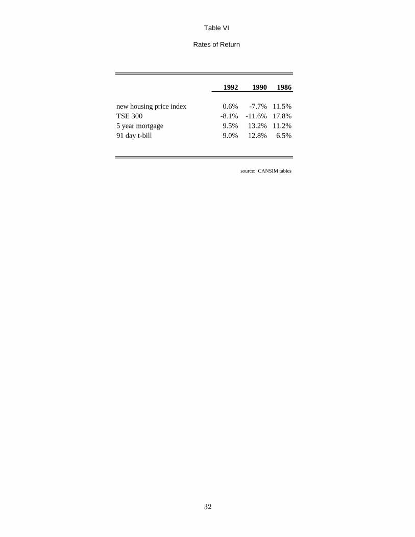
Table VI
Rates of Return
1992 1990 1986
new housing price index 0.6% -7.7% 11.5%TSE 300 -8.1% -11.6% 17.8%5 year mortgage 9.5% 13.2% 11.2%91 day t-bill 9.0% 12.8% 6.5%
source: CANSIM tables
32