SAVING OPENNESS AND GROWTH A PANEL DATA VAR …faculty.smu.edu/tosang/pdf/hoogstrate_osang.pdf · 5...

Saving, Openness, and Growth: A Panel Data VAR Approach 1

Chapter

SAVING, OPENNESS, AND GROWTH: A PANEL DATA VAR APPROACH

André Hoogstrate∗ and Thomas Osang∗∗

ABSTRACT

Using a country-level panel data set, we investigate the relationship between GDP growth, savings, and openness to trade in general and the link between openness and growth conditional on a country's savings rate in particular. We find that the current openness has a significant positive effect on GDP growth in all VAR models, even though the impact is small compared to the strong positive effect of current savings on growth. Based on the estimation of a threshold VAR model and the corresponding impulse response functions we find that for countries in the high savings regime, a shock to openness has a positive effect on GDP growth that is about three times the size of the growth effect for countries in the low saving regime, at least in the very short run. Keywords: endogenous threshold estimation, non-linear VAR, impulse response analysis.

∗ Ministry of Justice, Netherlands Forensic Institute, P.O. Box 3110, 2280 GC Rijswijk, The Netherlands. Tel:

+31-70-413-5142, Fax: +31-70-413-5454, E-mail: [email protected]. This research was sponsored by the Economics Research Foundation, which is part of the Netherlands Organization for Scientific Research (NWO).

∗∗ Corresponding author: Southern Methodist University, Department of Economics, Dallas, TX 75275, Tel: (214) 768-4398, Fax: (214) 768-1821, E-mail: [email protected].

André Hoogstrate and Thomas Osang 2

INTRODUCTION This paper brings together two important parts of the empirical literature on the

determinants of economic growth, namely growth and openness to trade on the one hand and growth and saving on the other. Over the last decade, numerous empirical studies have examined the relationship between growth and openness to trade (see, for example, Levine and Renelt (1992), Edwards (1993), Jorgenson and Ho (1993), Harrison (1996), Sachs and Warner (1995), and Frankel and Romer (l999)).1 Interestingly, the various studies yield conflicting results. While some find evidence for a strong positive effect of openness on growth (e.g. Sachs and Warner), others report a statistically insignificant or even inverse relationship between the two variables.2 In Ann Harrison's study, for example, only two of the six measures of openness are significant at the five percent level, while the sign of the trade share in GDP is negative though not significant (Table 6, p. 434). Furthermore, some studies find the estimated coefficient on openness to be sensitive to changes in the econometric model or data set. Levine and Renelt report that ''after controlling for the share of investment in GDP we cannot find an independent and robust relationship between any trade ... indicator and growth'' (p. 954).

In contrast to the results for the empirical relationship between openness and growth, the empirical literature provides solid evidence on the relationship between growth and saving (See, for example, Maddison (1992), Carroll and Weil (1993), and Bosworth (1993)). These studies find that countries with higher saving rates have significantly higher growth rates, a result that sensitivity tests show to be fairly robust (Levine and Renelt (1992), p. 946).3 The result that higher saving rates lead to higher long-term growth rates is also a key insight of the new growth literature.4

Interestingly, none of the empirical studies cited above considers in detail the triangular relationship between GDP growth, savings, and openness to trade including the obvious feedback effects between these variables, in particular the impact of openness on savings. By analyzing the relationship between these variables in a VAR framework, we take into account the potential endogeneity of variables such as openness and savings assumed to be exogenous in the typical cross-country growth regression. Furthermore, by using a panel data set instead of the usual cross-section approach, we are able to model the relationship between the three variables in both the time series and the cross section dimension. While panel data analysis in the empirical growth literature has been used before (see Harrison (1996)), it is still the exception. Finally, we also examine the potentially nonlinear relationship between GDP growth, openness, and saving. Such a nonlinear link has been the focus of a number of recent

1 Possible channels through which openness to trade may affect long-run growth are: access to lower priced

foreign capital goods; access to foreign intermediate inputs; removal of domestic bottlenecks to growth; access to foreign knowledge, etc.

2 It is interesting to note that the theoretical literature on trade and endogenous growth also comes out on both sides, although it seems that the majority of papers predict a positive relationship. See Lee (1995) and Turnovsky (1996), among others. For an overview of the endogenous growth literature in both open and closed economies, see Aghion and Howitt (1998).

3 Levine and Renelt show that the relationship between the investment share in GDP and GDP\ growth is strong and robust. Since it is well known that investment and saving rates are highly correlated within countries (see Gordon and Bovenberg (1996) for a recent investigation of this empirical regularity), we interpret their findings as indirect evidence for a robust link between saving and GDP\ growth.

4 See, again, Aghion and Howitt (1998).


theoretical models on trade and endogenous growth. These models indicate that certain model parameters linked to the consumption and savings behavior of households may play a key role in the interaction between growth and openness (Feenstra (1996), Kwark (1996), and Osang and Pereira (1996)). Feenstra shows that the instantaneous elasticity of substitution plays an important role for the interaction between trade and growth, while Kwark and Osang and Pereira point out that there exists a threshold level of the intertemporal elasticity of substitution that separates growth-enhancing from growth-reducing regimes of increased openness to trade.5 Since the intertemporal elasticity of substitution is a key parameter for saving in the endogenous growth literature, it seems naturally to test the hypothesis that the relationship between openness and growth changes once the saving rate exceeds a certain endogenously determined threshold level.

In order to tackle the above issues empirically, we proceed as follows. We first estimate a linear (non-threshold) VAR as a benchmark model and derive the impulse response functions for this case. We then test for the existence of a threshold saving rate separating high from low saving regimes. Based on these results, we estimate the threshold VAR model and derive the impulse response functions that correspond to each regime. The data set used in our analysis consists of 59 countries for the period from 1960 to 1995.

The main findings of the paper are as follows. First, we find that current openness has a statistically significant positive effect on GDP growth in all VAR models, even though the impact is relatively small compared to the strong positive effect of current savings on growth. Second, based on the linear VAR estimates, the impulse response functions show that a shock in openness has a positive and statistically significant effect on GDP growth although the impact is relatively small both given the size of the shock and relative to a shock in savings. Nevertheless, it is worth noting that, by applying a VAR approach to a panel data set, we find a positive effect of openness to trade on GDP growth. This result is independent of, and in addition to, the positive effect of savings (or investment) on GDP growth, a result that is in contrast to the findings of Harrison (1996) and Levine and Renelt (1992). Third, using different threshold test statistics we show the existence of an endogenous threshold separating high from low savings regimes. Finally, we find that the level of savings in a country indeed matters for the link between openness and growth. There are striking differences in both the estimation results and the impulse response functions between the two regimes. Among others, we find that a positive shock in openness leads to higher GDP growth in the first period but not in the subsequent periods in the high saving regime, while in the low savings regime the effect on GDP growth is substantially smaller in size in the first period but remains positive for a couple of periods. A similar result holds for the relationship between a shock in openness to trade and the response in the level of savings. While our results do not provide empirical evidence for the theoretical prediction that countries with low saving rates may actually see their GDP growth rates reduced as the result of increased exposure to foreign

5 A possible non-linear mechanism through which openness affects growth is as follows (see Osang and Pereira

(1996) for details). International differences in preferences and/or technologies lead to different steady state growth rates across countries. Assuming balanced trade and complete specialization, increasing the volume of trade (e.g. due to lower trade barriers or changes in consumer preferences) induces changes in the terms of trade. In this situation it is likely that a country with the weak attitude toward saving will experience an improvement in its terms of trade and, in turn, a decline in output growth, while a country with a strong saving performance will experience the opposite effect.


trade, the existing differences can nevertheless be interpreted as empirical evidence for a non-linear relationship between GDP growth, savings, and openness to trade.

The paper extends the existing literature in several ways. By estimating a VAR model instead of the standard single-equation approach we control for the feedback effects between the three variables. We employ a dynamic panel data model instead of the widely used cross-section analysis. We estimate the potentially non-linear relationship between saving rates, openness to trade, and growth, while the existing literature uses a linear relationship at best. Finally, estimating an endogenous threshold in a dynamic model raises some interesting questions concerning the underlying econometric theory since the estimation model is not well defined in the case of a non-existent threshold level. Most importantly, we use threshold test statistics recently developed by Andrews et al. (1996), Andrews and Ploberger (1994), and Hansen (1996, 2000) and modify them so that they can be applied to the case of a dynamic panel. To our knowledge, this is the first paper that uses these threshold tests in a dynamic panel data context.

The remainder of the paper is organized as follows. Section 2 describes the empirical model. Issues pertaining to the econometric methodology are discussed in section 3. Section 4 describes the data, while section 5 contains the empirical results. Section 6 concludes the paper.

THE EMPIRICAL MODEL The recent theoretical literature on endogenous growth in open economies suggests that

long-run GDP growth mainly depends on the following model parameters: − Technology parameters such as total factor productivity, A, and scale elasticities, α. − Taste parameters such as the intertemporal elasticity of substitution, σ, and the

discount rate, ρ. − Trade policy parameters, τ, representing both tariffs and non-tariff barriers to trade.6 The relation can thus be written as

( , , , , ).growth f A α σ ρ τ= (1) Unfortunately, we lack data that directly measure these parameters, especially over time

and for large sets of countries. Following the empirical growth literature, we approximate these parameters with data that are available across both countries and time.

Taste parameters reflect a country's willingness to postpone current consumption and determine the domestic supply of financial capital. Advanced production technologies are intensive in both physical and human capital and correspond to high levels of total factor productivity. Advanced production technologies are a major factor behind the domestic demand for financial capital. Given the fact that international capital is not sufficiently mobile

6 To simplify matters, we abstract from domestic fiscal and monetary policy parameters which also may affect

long-run growth rates.


(see, again, Gordon and Bovenberg (1996)) it seems reasonable to use the domestic saving rate of a country as a proxy for both sufficient supply and adequate demand in the market for financial capital. For ease of exposition, we restrict our attention to trade policy parameters which can be approximated either directly through some index of trade liberalization using country sources on trade barriers (see, for example, Thomas et al (1991) or indirectly through measures such as the black market premium in the currency market or an index measuring price distortions for consumption goods.7 Another widely used indirect measure for trade barriers is the ratio of exports plus imports to GDP. This proxy has the advantage that it is available for many countries for at least three decades. It is also relatively free of different definitions and data collection techniques between countries. Furthermore, Harrison (1996) shows that it has the highest correlation coefficient with trade reform compared to all other indirect openness measures (Table 2, p. 429). Its most severe disadvantage is that its value does not depend on trade barriers alone but may also depend on country size or foreign direct investment.8 However, most of the empirical analysis below uses differenced data. Since differenced trade shares are essentially uncorrelated with country size, the criticism does not apply here. Therefore, we use the share of trade in GDP as proxy for a country's openness to trade. This choice as the additional advantage that it allows us to directly compare our results with results from earlier studies. Finally, as in Harrison (1996), we assume that the technology parameters can be incorporated in the function f . This leaves us with the following estimable model for long-run growth:

( , ) with 0; 0,s ogrowth f s o f f= > > (2)

where s indicates the saving rate and o the level of openness. The sign of the partial derivatives reflects the predictions from the majority of theoretical models. Note that (2) is also a common result in the endogenous growth literature where output growth can be expressed as a function of the (endogenous) savings rate of the economy. Since (2) expresses a long-run equilibrium condition which may not hold exactly in the short run due to exogenous shocks, it is important to include dynamics in our empirical model. For this reason and because the functional form of f is unknown we use an unrestricted linear first-order VAR model as an approximation of (2),

, 1 , 1 , ,i t i t i tX c A X ε−= + + (3)

with , , , ,( , , )i t i t i t i tX O S Y ′= Δ where

, i tYΔ denotes GDP growth of country i at time t, ( , , , 1log( ) log( )i t i t i tY Y Y −Δ = − ).

7 See Harrison (1996) for other indirect measures of trade barriers as well as a detailed dicussion of measurement

problems associated with both direct and indirect proxies of trade barriers. 8 A refined trade share measure which is independent of country size is implied by a recent paper by Eaton and

Kortum (1999). A comparison between this new measure and the measure used in this study for the relationship between openness and growth is the topic of a separate paper we are currently working on.


,i tS denotes the gross domestic savings rate of country i at time t,

,i tO denotes the log ratio of imports plus exports to GDP of country i at time t,

and the disturbance term ,i tε is assumed to be independent Gaussian with E( ,i tε ) = 0 and

covariance , ,( )i t i t iE ε ε ′ = Ω . It is well known that the estimates of the structural parameters

of the VAR model are not independent of the ordering of the variables in ,i tX . The ordering

we have chosen is such that GDP growth is affected by contemporaneous changes of the other two variables, while openness to trade is only affected by lagged values of all variables. Given our definition of openness this seems to be sensible assumption which is also in line with the formulation of the GDP growth equation in Harrison (1996).

We assume that the intercept c in equation (3) captures the effects of the technology parameters. The assumption that c is identical across countries is rather restrictive. In section 5 below, we relax this assumption whenever possible and carefully compare the results between pooled and fixed effects models. Unfortunately, at this moment there is no technique available to determine an endogenous threshold in a dynamic panel data context with individual effects. However, a test statistic for a non-dynamic panel data model with individual effects was recently proposed by Hansen (1999). We discuss this test statistic and its application to our model in Section 5 as well. Because we are also interested in the contemporaneous effects (assuming them to be the same for each individual country), we rewrite (3) in the following structural form

, 0 , 1 , 1 ,i t i t i t i tX B X B X uμ −= + + + (4)

where ,i tu is again independent Gaussian with zero mean but with diagonal covariance matrix

2 2 2, , ,1 ,2 ,3( ) ( , , )i t i t i i i iE u u diag σ σ σ′ = ≡ Λ , where i i ′Ω = ΓΛ Γ and Γ is lower triangular

with ones on the main diagonal. We then have 1cμ −= Γ , 10 ( )B I −= − Γ and 1

1 1B A−= Γ .

Observe that 0B is lower triangular with zeros on the main diagonal.9 As described above, a number of recent endogenous growth models predict a non-linear

relationship between GDP growth, saving, and openness to trade. The long-run growth model based on these papers can be written as:

( , ) with 0; 0 iff s ogrowth f s o f f s γ> >= >

< <, (5)

where γ is the benchmark value of the saving rate that separates high- and low-saving regimes. To test the hypothesis that the relation between openness and GDP growth changes if the savings level exceeds a certain level we contrast the benchmark model in (4) with the following threshold VAR model:

9 For further details on the problem of identification, see Lütkepohl (1991).


, 0 , 1 , 1 , 1( ) ( )i t i t i t i tX B X B X I Sμ γ− −= + + ≤ (6)

0 , 1 , 1 , 1 ,( ) ( )i t i t i t i tB X B X I Sμ γ ω− −+ + + > +

where , 1( )i tI S γ− > is an indicator function which equals one when the inequality holds and

zero otherwise. Note that the threshold parameter γ is unknown and needs to be estimated as

well. The use of , 1i tS − instead of ,i tS in the indicator function allows us to consider the

savings level pre-determined. We proceed by introducing tests for the existence of an endogenous threshold as well as recently developed techniques for estimation of (6).

ECONOMETRIC CONSIDERATIONS The econometric analysis of the above models requires a number of non-standard

techniques which are discussed in detail in this section. In particular, we discuss the following topics: tests for the existence of a threshold, estimation and inference of the threshold VAR model, and nonlinear impulse response analysis.

The econometric analysis of the benchmark VAR model (4) is essentially the analysis of a vector autoregressive model with pooled coefficients. This analysis is similar to that of a large VAR with restrictions on the coefficients of the lag polynomial. Since we assume T to be large we can apply the standard asymptotic theory on stationary vector autoregressions taking into account the pooling restrictions.10

Testing for the Existence of a Threshold To test for the existence of a threshold we choose the following setup. Let the observable

variables be denoted by ( , )i iY X for 1,...,i N= . iX is a (1 )xk× vector and iY is a scalar variable. Let the following relation hold:

1 2Y ( )i i i i iX Z I qβ γ β ε= + > + (7)

where iZ is a (1 )zk× vector, iq is a one dimensional variable and γ is a scalar which we

assume to be contained in a compact subset Γ of R. We assume that the variables in iZ are

also contained in iX i.e., iZ is a subvector of iX and thus observable as well. Finally, we

assume iε to be a zero mean i.i.d distributed random variable with finite variance 2σ . As noted above, I(.) denotes an indicator function which determines a possible break between observations satisfying the inequality condition and those not satisfying the condition.

10 See Lütkepohl (1991) or Hamilton (1994) for an introduction to this analysis.


The main problem with threshold test statistics is that under the null hypothesis of no

threshold (i.e. 0 0 1 1, , )B B B Bμ μ= = = , the threshold parameter γ is not identified, and

we therefore cannot apply standard hypothesis testing theory. To address this issue, we use recently developed test statistics (see Andrews, Lee and Ploberger (1996), Andrews and Ploberger (1994) and Hansen (1996, 2000). Some of these test statistics were designed for time series and/or cross section data, in which case we modify them for the case of a panel data set.

Estimation and Inference on the Threshold If the above test statistics lead us to conclude that a threshold exists, we continue by

estimating the threshold, γ , as well as the other coefficients of the model, namely 1β and

2β The estimators for γ , 1β and 2β are the solution to the following nonlinear least squares problem:

1 21 2 1 ( ) 2 1 ( ) 2, ,

ˆ ˆˆ( , , ) arg min ( ) ( )Y X Z Y X Zγ γγ β βγ β β β β β β

∈Γ′= − − − − .

Finding the global minimum can be achieved in two steps. First, we minimize the sum of

squared errors for a fixed γ . Applying OLS gives us an estimate of the variance of the

residuals, 2ˆ ( )σ γ . Second, we minimize 2ˆ ( )σ γ over all γ ∈Γ . The final estimates are then

the OLS coefficients corresponding to the γ which minimizes 2ˆ ( )σ γ . Note that when the

iε are i.i.d 2(0, )N σ , this estimator is also the MLE. As is known from the literature (see, for example, Bai (1995), Picard (1985), and Chan

(1993)), the estimator for γ has a convergence rate of order n, which is much faster than the

order of convergence n for the other parameters of the model. The derivation of the asymptotic distribution of the estimator for γ is rather difficult, in particular when the change

between 1β and 2β is considered to be fixed or relatively large. In this case the distance

between the two parameters appears in the asymptotic distribution for γ which makes inference results almost impossible. However, under the assumption of a local alternative, i.e. a small difference between 1β and 2β , Hansen (1996) is able to derive the asymptotic

distribution of the Likelihood Ratio test statistic for 0γ γ= . He then uses this result to construct a confidence interval for γ . The confidence intervals presented in Table 1 and 4 below are based on his procedure.


Nonlinear Impulse Responses Computing impulse response functions for nonlinear dynamic models is more

complicated than computing impulse response functions for linear dynamic models for several reasons. Most complications arise from the fact that there are no analytical results in the nonlinear case. This means that the impulse responses must be obtained numerically or need to be simulated. Further, it is much harder to present and investigate all the information contained in the impulse response of a nonlinear system. This is due to the fact that the response of a nonlinear system to a shock at time 0t is path-dependent in a nonlinear way, i.e., it depends on the observations before the shock enters the system and on the disturbances which enter the system between time 0t and 0t k+ . Finally, the proportionality of a response to the size of the shock in a linear system does not hold in a nonlinear system.11

For the linear VAR we present the traditional impulse responses, including 2 standard-errors confidence bounds, based on 500 drawings from the distribution of the estimates of the parameters.

For the nonlinear threshold VAR we estimate an impulse response function corresponding to the Generalized Impulse Response function proposed by Potter (1995) and Koop, Pesaran, and Potter (1996):

0 0 0 0 0 00 1 1 1( , , , ) ( | , ) ( | )t t k t t t k tGI t k E X E Xδ ε δ− + − + −Ω = Ω = − Ω ,

where

0 1t −Ω is the history at time 0t , and δ is the shock given to the system at time 0t . To

obtain this impulse response function we need to integrate out the future shocks

0 01 ,...,t t kε ε+ + , that is

0 1 0 0 0 0 00 00 1 ,..., 1 1 ( , , , ) ( ( | , , ,..., )t t kt t k t t t t kGI t k E E Xε εδ ε δ ε ε+ +− + − + +Ω = Ω = (8)

0 0 0 01 1( | , ,..., ))t k t t t kE X ε ε+ − + +− Ω .

To do this we generate a large number of future zero mean i.i.d. normal shocks

0 01 ,...,i it t kε ε+ + , i = 1,...,R, and replace

00 1( , , , )tGI t k δ −Ω by

0 0 0 0 0 00 1 1 11

1 ( , , , ) ( | , , ,..., )R

i it t k t t t t k

iGI t k E X

Rδ ε δ ε ε− + − + +

=

Ω = Ω =∑%

0 0 0 01 11

1 ( | , ,..., )R

i it k t t t k

iE X

Rε ε+ − + +

=

− Ω∑

11 Further details on the issue of nonlinear impulse response analysis can be found in Gallant, Rossi and Tauchen

(1993) and Potter (1995).


i.e., we average the impulse response function over the future shocks. Next we notice that

00 1 ( , , , )tGI t k δ −Ω% depends on 0 1t −Ω . In a threshold model it makes a big difference

whether the system is close to the threshold level at 0t , the time of the shock, or not.

Therefore, we consider 00 1 ( , , , )tGI t k δ −Ω% conditional on different histories

0 1t −Ω . In our

case we are especially interested in the behavior of the system for the high and low saving regimes. Therefore, we calculate

00 1( , , , )tGI t k δ −Ω% , for the following three situations:

unconditional on the regime we are at time 0t , conditional on being in the high saving regime

at time 0t , and conditional on being in the low saving regime at time 0t . For each of the three situations we generate 2000 histories, simulate the model, and leave

out the first 500 observations to avoid initial observation problems. For each individual history we calculate the generalized impulse response function based on 50 sets of future shocks. Since the impulse response function of a threshold model can be asymmetric, we investigate both negative and positive unit shocks. We present figures for each of the three classes of histories. Each graph presents the average impulse response function as well as the 95% most centered realizations.

THE DATA All data are taken from World Bank publications (1996), (1997). GDP growth is the log

difference of real per capita GDP in constant 1987 value of the local currency. The saving rate is the ratio of nominal gross domestic savings to nominal GDP (both in local currency), while openness to trade is the ratio of nominal exports plus imports to nominal GDP (both again in local currency). These data are available for all OECD countries as well as a large number of developing countries. In our sample of 59 countries, high-income, middle-income and low-income countries are roughly equally represented. Non-market economies as well as countries with a population of less than one million (in 1995) are excluded.12 The sample period ranges from 1960 to 1995.

Figure 1 displays the empirical distributions of the data. Clearly, the saving rate displays a good deal of variability which is necessary to verify our hypothesis of a changing relation between output growth and openness. Without such variability, testing and estimation of a threshold level of saving would be futile.

12 The countries in our sample are: Algeria, Argentina, Australia, Austria, Bangladesh, Belgium, Bolivia, Brazil,

Canada, Chile, Colombia, Congo, Costa Rica, Cote d'Ivoire, Denmark, Egypt, El Salvador, Finland, France, Germany, Ghana, Greece, Guatemala, Hong Kong, India, Indonesia, Ireland, Israel, Italy, Jamaica, Japan, Kenya, South Korea, Madagascar, Malaysia, Mauritius, Morocco, Netherlands, New Zealand, Nigeria, Norway, Pakistan, Panama, Paraguay, Peru, Philippines, Portugal, Senegal, Singapore, South Africa, Spain, Sri Lanka, Sweden, Switzerland, Thailand, Turkey, United Kingdom, United States, and Uruguay.


Figure 1. Distribution of the data; frequencies are given on the vertical axis.

EMPIRICAL RESULTS

Long-run Effects We first consider the long-run relation between the saving rate, openness to trade, and

GDP growth. Using time-averaged variables for each country, i.e.,

, ,1 1, i i t i i tt t

Y Y S ST T

Δ = Δ =∑ ∑ and ,1

i i ttO O

T= ∑ , where T denotes the time

dimension of the sample, simple OLS yields the following result:

2 0.003 0.115 0.005 0.31, 59

(0.006) (0.028) (0.003)

i i iY S O R NΔ = + + = = (9)


Clearly, the effect of openness is small and insignificant. Misspecification tests show that we cannot reject normality nor homogeneity of the residuals (White's test yields

2 18.29R = ). Next we test for the existence of a threshold. We calculate three LM tests (denoted by

aveLM, expLM, supLM) as well as Hansen's F-test (1996) (denoted by HansenF). Since the regressors are averages over time, the threshold at a certain time would be conditioned on future values of the regressors producing inconsistent estimates. To avoid this problem we use the saving rate of 1960 as the threshold variable.

Table 1. Threshold Tests and Estimation: Long-Run Growth Model

Test Statistic p-value

expLM 7.04 p < 0.01 aveLM 12.36 p < 0.01 supLM 18.74 p < 0.01 HansenF 29.66 0.000 Estimate of threshold 95% conf. interval γ 0.164 (0.151, 0.235)

Table 1 contains the values for the four test statistics and their corresponding p-values.

The threshold estimate and its 95% confidence interval as derived from Hansen's testing procedure are also given. The trimming percentage π for all tests is 10%. Lower values for π do not lead to different estimates of the threshold. All tests reject the null of no threshold at the 1% significance level. The resulting estimate for the threshold is 0.164. We use this value to split the sample and reestimate the above equation for each subsample. For the low savings countries ( 0.164γ ≤ ) we find

2 0.011 0.216 0.001 0.63, 29

(0.008) (0.034) (0.004)

i i iY S O R NΔ = − + + = = (10)

and for the high savings countries ( 0.164γ > ) we obtain

2 0.007 0.118 0.0003 0.23, 30

(0.013) (0.052) (0.004)

i i iY S O R NΔ = − + − = = (11)

with a joined 2 0.56R = . Interestingly, the sign of the coefficient for openness varies between the two subgroups of countries, but both signs are insignificant. Also, compared to the benchmark model, the estimated coefficient for the average saving rate is larger for both subgroups.


VAR Analysis: Estimation, Identification and Testing Before we estimate any VAR model we need to investigate the stationarity of each

variable. For this we use the panel unit root test statistics recently developed by Im et al. (1996). This unit root test, specifically designed for heterogeneous panels, is specified as:

, , 1 ,(1 )i t i i i i t i tx xφ μ φ ε−= − + +

where 2

,( )i t iE ε σ= . The hypothesis 1iφ = for all i is tested against 1iφ < for all i. Since

we impose that iφ φ= and iμ μ= for all i in our model, we can use this procedure to test for unit roots. Furthermore, since their test is not based on these restrictions, it makes our results robust against this type of misspecification.

Table 2. Test for Unit Roots

Variable LR26(0,0) p-value

GDP growth 37.97 0.000 saving rate 4.51 0.000 openness -0.11 0.454

The results, given in Table 2, indicate that we can reject the hypothesis of a unit root in

GDP growth and the saving rate. For openness, however, we cannot reject the unit root null making first differencing a necessity to obtain stationarity. We thus use

, , , 1ln lni t i t i tO O O −Δ = − instead of ,i tO in all subsequent testing and estimation

procedures.13 We present the estimation results for the linear VAR model (4) in Table 3.14 Note that the results presented in the table as well as all subsequent estimation results and test statistics are based on transformed data. The transformation which removes the cross-country heterogeneity in the data is necessary because the threshold test statistics presented below are only valid for homoscedastic disturbance terms. To ensure compatibility between the test statistics and the estimates of the different VAR models, the latter are based on the transformed data as well.

In the first regression (with GDP growth as the dependent variable) all explanatory variables except for the constant and the lagged change in openness are significant at the 5% level. It is interesting to note that change in openness has a positive contemporaneous effect on GDP growth. As the next column in Table 3 reveals (with the savings rate as the dependent variable) a change in openness has a significant positive impact on the savings rate. Therefore, a change in openness has also a positive indirect impact on GDP growth through its effect on savings. All other explanatory variables including the constant are also significant at the 5% level. In the third regression (with the change of openness as dependent

13 Note that using first differences instead of the level of openness changes the correlation coefficient between

openness and country size from -.42 to .17. 14 Using Akaike's information criterion as well as the final prediction error criterion, we find that the optimal VAR

lag length is unity. The result can be obtained from the authors upon request.


variable) all variables except for the constant are insignificant at the 5% level although lagged GDP growth is positive and significant at the 10% level.

Table 3. Estimation results: Linear VAR

Dependent Variable:

Regressors ,i tYΔ ,i tS ,i tOΔ

c 0.001 (0.002)

0.008* (0.001)

0.018* (0.006)

,i tS 0.499* (0.041) -- --

,i tOΔ 0.035* (0.009)

0.013* (0.006) --

, 1i tY −Δ 0.358* (0.024)

0.071* (0.016)

0.108 (0.059)

, 1i tS − -0.436* (0.042)

0.953* (0.007)

-0.036 (0.026)

, 1i tO −Δ -0.009 (0.008)

0.012* (0.006)

0.03 (0.029)

N = 1947 2 0.39R = 2 0.98R = 2 0.01R = * significant at 5% level. Note: Heteroscedasticity consistent standard errors in parentheses.

Next, we test for the existence of a threshold in the VAR system using the same tests as

presented in Table 1. In a VAR system there are two ways to test for the existence of a breakpoint. A threshold test can be performed separately for each of the three equations. Not surprisingly, we may find a different threshold estimate for each equation in this case. Alternatively, we can restrict the test statistic so that the threshold will be the same for all equations. We pursue both approaches and present the results in Table 4.

Table 4. Threshold Tests and Estimation: VAR Equations

Threshold Test Statistics Unrestricted VAR Restricted VAR

,i tYΔ ,i tS ,i tOΔ

expLM 22.96* 17.59* 12.75* 54.61*

aveLM 25.60* 25.25* 13.66* 65.96*

supLM 52.92* 42.14* 33.08* 118.42*

HansenF 57.14* 46.67* 27.18* 66.50*

Threshold Estimation γ 0.184 0.241 0.205 0.188

95% conf. inter. (0.162, 0.194)

(0.196, 0.243)

(0.183, 0.217) (0.178, 0.204)

* significant at 1% level.


All test are based on trimming percentage of π = 0.10. Clearly, all four tests confirm the existence of a threshold at the 1% significance level. To further test for the existence of a threshold, we also calculate a new test statistic proposed by Hansen (1999). The new test allows to test for one (or more) thresholds in the context of a non-dynamic panel with individual specific effects. The estimated equation for this test is thus

, 0 1 , 1 2 , 1 ,i t i i t i t i tY S Oβ β β ε− −Δ = + + Δ +

The trade-off between this and the previous test statistics is clear: the new test statistic

allows for individual effects at the expense of excluding lagged dependent variables. The results are presented in Table 5.

Table 5. Threshold Test and Estimation: Non-dynamic Panel with Fixed Effects

Threshold Test Statistic

Hansen F 15.62 p-value 0.15

Threshold Estimation γ 0.214 95% conf. inter. (0.105, 0.245)

Note: Dependent variable: ,i tYΔ . The results indicate that in the context of a non-dynamic panel with fixed effects, the

existence of a threshold cannot be rejected at the 15% level.15 The significance level is somewhat higher than in the previous test results. However, the estimated threshold of 21% is very close to the estimate from Table 4. We therefore conclude that there is sufficient evidence for the existence of a threshold both with and without fixed effects. In the absence of a reasonable economic interpretation for the different threshold values, we base our subsequent analysis on the threshold estimate from the restricted VAR in Table 4. Based on the threshold level of 0.19, we estimate the resulting threshold model. The results are presented in Table 6 (robust standard errors are in parentheses).

There are 798 observations in the low savings regime and 1149 observations in the high savings regime. While eight countries are in the low saving regime at every point in time, 13 countries are always in the high saving regime. All other countries switch regimes at least once during the sample period.

15 There is no evidence for additional thresholds. The p-values for a second and third threshold are 39% and 55%,

respectively.


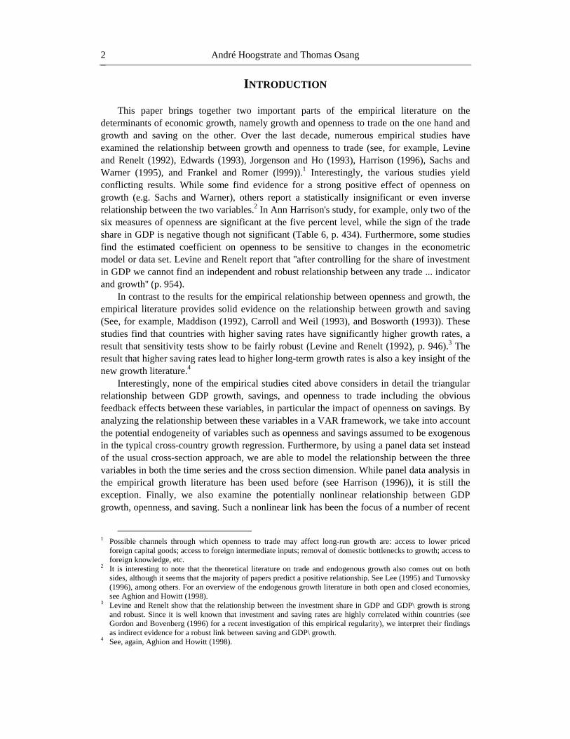
Table 6. Estimation Results: Threshold Model

, 1 0.19, 798i tS N− ≤ = , 1 0.19, 1149i tS N− > =

Dependent Variable: Regressors

,i tYΔ ,i tS ,i tOΔ ,i tYΔ ,i tS ,i tOΔ

c 0.002 (0.004)

0.009* (0.002)

-0.004 (0.001)

-0.009* (0.004)

0.008* (0.003)

-0.032* (0.012)

,i tS 0.323* (0.051) -- -- 0.608*

(0.057) -- --

,i tOΔ 0.024* (0.01)

-0.002 (0.008) -- 0.045*

(0.014) 0.027* (0.008) --

, 1i tY −Δ 0.367* (0.056)

0.032 (0.025)

-0.112 (0.102)

0.3421* (0.033)

0.092* (0.019)

0.231* (0.075)

, 1i tS − -0.25* (0.056)

0.95* (0.017)

0.161* (0.082)

-0.505* (0.047)

0.951* (0.012)

-0.108* (0.047)

, 1i tO −Δ 0.017 (0.01)

0.033* (0.009)

-0.027 (0.048)

-0.032* (0.011)

-0.007 (0.008)

0.07* (0.035)

2 0.30R = 2 0.93R = 2 0.01R = 2 0.41R = 2 0.98R = 2 0.023R =* significant at 5% level. Note: heteroscedasticity consistent standard errors in parentheses.

There are a number of important differences in the sign and size of the estimated coefficients between the two regimes. In the high savings regime, the positive contemporaneous effect of savings on GDP growth is roughly twice the size of the effect for countries in the low saving regime. A similar result holds for openness and growth: in the high saving regime, the direct contemporaneous effect of openness to trade on GDP growth is twice the size of that for the low saving regime. In addition, the indirect effect (through savings) is positive for the high savings regime but negative (though not significant) for the low saving regime. With regard to the impact of lagged variables, the situation is different. The direct effect of lagged openness of growth is negative for the high saving regime but positive though not significant for the low saving regime, while the indirect effect through savings is positive (though insignificant) for the high saving regime but negative for the low saving regime. Also, the lagged variables in the change in openness regression have opposite signs when compared across regimes. In particular, saving has a significant negative impact on openness growth in the high saving regime, but its impact is positive (significant at the 5% level) in the low saving regime.

To check the robustness of the estimates in Table 6 we also estimate a number of fixed effects models. To conserve space, we only present the results for the GDP growth equation of the VAR.16 Adding fixed effects to the linear VAR is not a problem as long as one takes account of the endogeneity problem created by the lagged dependent variable in the presence of country specific effects. To address this problem, we use the panel IV estimator presented in Anderson and Hsiao (1981) using GDP growth lagged twice ( , 2i tY −Δ ) as the instrument for

lagged change in GDP growth. In the nonlinear VAR, the Anderson-Hsiao estimator can only be applied to two subsets of countries, namely to those countries which have savings rates

16 The corresponding results for the other VAR equations can be obtained from the authors upon request.


that are either always above or always below the threshold. For all other countries, the time series data are no longer continuous in the nonlinear VAR case which precludes the use of the Anderson-Hsiao IV estimator. For a threshold value of 19%, there are 8 countries in the 'always below' and13 countries in the 'always above' regime.17 The test results for the IV estimator with fixed effects are presented in Table 7.

Table 7. Estimation Results: IV Estimator with Fixed Effects

All countries Countries with ,i tS

below threshold

Countries with ,i tS

above threshold

Regressors Dependent Variable: , 1i tY −ΔΔ

,i tSΔ 0.422* (0.05)

0.419* (0.113)

0.717* (0.114)

,i tOΔΔ 0.025* (0.009)

0.05* (0.016)

0.058* (0.02)

, 1i tY −ΔΔ 0.241* (0.059)

0.185 (0.132)

0.31* (0.129)

, 1i tS −Δ -0.438* (0.046)

-0.177 (0.111)

-0.876* (0.103)

, 1i tO −ΔΔ -0.028* (0.009)

0.008 (0.02)

-0.044* (0.014)

2 0.026R =% 2 0.006R =% 2 0.232R =% N = 1947 N = 264 N = 429

* significant at 5% level. Note: heteroscedasticity consistent standard errors in parentheses.

Comparing the results from Table 7 with the appropriate columns from Tables 3 and 6,

we notice that all estimated coefficients have the same sign and that the difference in size between most estimates is minimal.18 The biggest difference arises in the estimation of the coefficient on lagged GDP which is smaller in the IV regressions. However, since this is the variable which we instrument for, the availability of better instruments may also lead to estimates which are closer to the estimate from the pooled regression. Overall, we consider the similarity between the pooled and the fixed effect IV estimates in both the linear and the non-linear VAR as evidence for the empirical validity of pooling. We therefore proceed by using the estimates from the pooled VAR models for the derivation of the impulse response functions discussed in the next section.

17 The 'always below' countries are: Bangladesh, Egypt, Ghana, Guatemala, Israel, Madagascar, Pakistan, and

Senegal; the 'always above' countries are: Australia, Austria, France, Germany, Hong Kong, Italy, Japan, Malaysia, Netherlands, New Zealand, Norway, Spain, and Switzerland.

18 Note that, due to the lack of a constant in the IV regressions, 2R has been replaced with the squared correlation

between actual and predicted values of the dependent variable, 2R% , as a measure of goodness of fit.


VAR Analysis: Impulse Responses The impulse response analysis is based on the coefficient estimates presented in Table 3

for the linear model and in Table 6 for the nonlinear threshold model. Observe that the threshold tests presented in the previous section indicate the existence of

a threshold even if only one of the coefficients of μ , 0B or 1B changes significantly between the two regimes. Clearly, in this case one could obtain efficiency gains by restricting all other coefficients to be the same. Since we do not restrict the coefficients in this way, a potential efficiency loss is possible, not only for the coefficient estimates but for the impulse response functions as well. However, any potential efficiency loss does not affect the validity of our analysis or the possible outcomes.

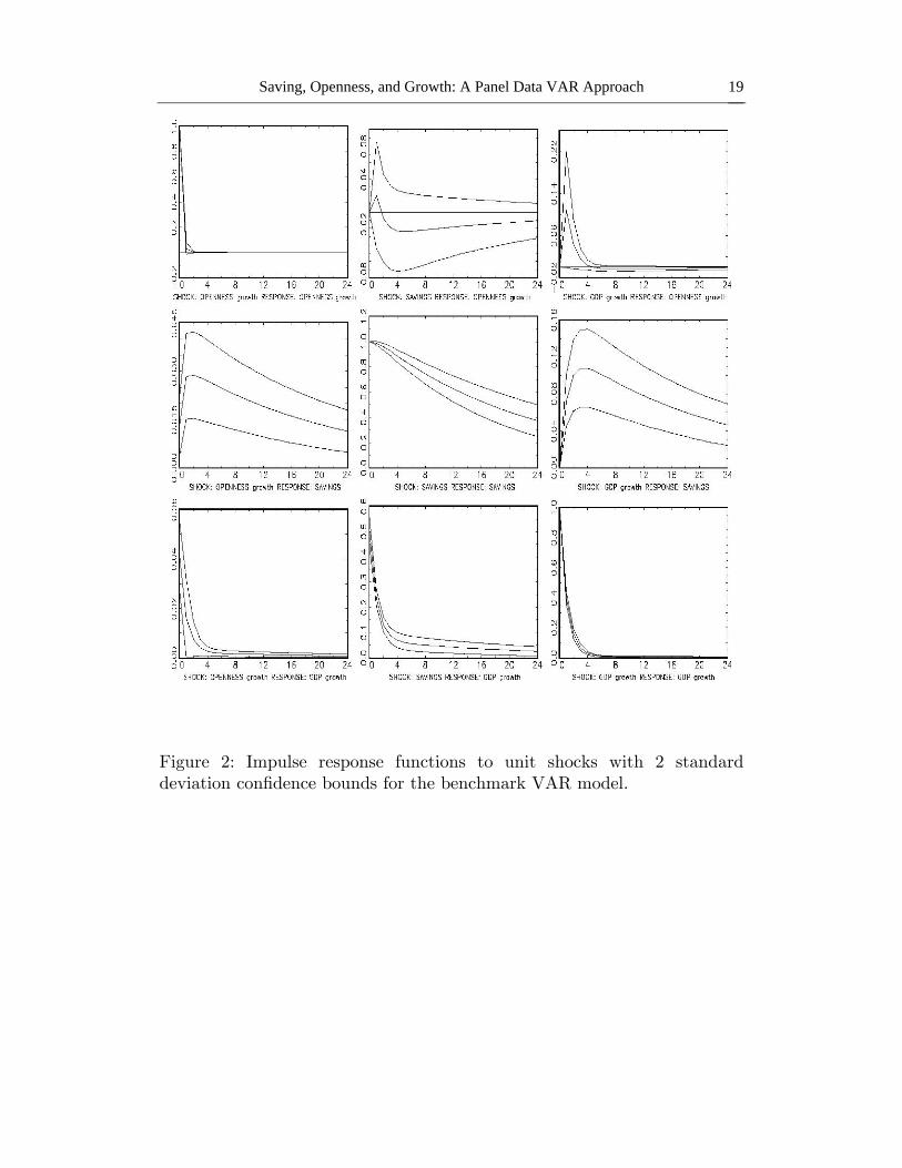
We start by analyzing the impulse responses to unit shocks in the linear model. Recall that in our model the innovations are already orthogonal. The impulse responses for the linear VAR from Table 3 are given in Figure 2. Due to the symmetry of the linear VAR, only positive shocks are being presented. Observe that there are statistically significant positive responses of both GDP growth and savings to a shock in openness growth. However, given the size of the shock, the size of the response is small. In addition, the positive effect on GDP growth is short-lived and becomes insignificant after a few periods. As expected, a shock in savings elicits a strong positive reaction of output growth which remains significant in all subsequent periods. Interestingly, the change in openness turns negative after a few periods as a result of a savings shock. A GDP growth shock has a short though barely significant effect on openness growth, while the positive impact of a GDP growth shock on savings is significant in all periods except for the first.

For the analysis of the nonlinear impulse responses we use one- or two-standard-

deviation shocks instead of unit shocks. The use of smaller shocks is required here in order to avoid that strong shocks force the system to be always in the low or high saving regime regardless of the starting level of savings. Figures 3 to 5 present the average nonlinear impulse responses as well as the 95% most centered realizations to positive and negative shocks in openness growth depending on the starting level of savings. Figure 3 gives the results unconditional on whether the starting level of savings is above or below the threshold, Figure 4 conditional on the level being above, and Figure 5 conditional on the level being below the threshold. In each figure, the first row gives the responses to a positive shock, while the second row traces the effects of a negative shock.


Figure 2: Impulse response functions to unit shocks with 2 standard deviation confidence bounds for the benchmark VAR model.


Figure 3: Impulse response functions (average and 95% most centered real-izations) to a one-standard deviation shock in openness growth for threshold VAR model: initial saving rates unconditional on saving regime


Figure 4: Impulse response functions (average and 95% most centered real-izations) to a one-standard deviation shock in openness growth for threshold VAR model: initial saving rates conditional on high saving regime


Figure 5: Impulse response functions (average and 95% most centered real-izations) to a one-standard-deviation shock in openness growth for threshold VAR model: initial saving rates conditional on low saving regime


Figure 6: Average impulse response functions to a one-standard deviation shock in openness growth for threshold VAR model: initial saving rates conditional on high saving regime


Figure 7: Average impulse response functions (average and 95% most cen-tered realizations) to a one-standard-deviation shock in openness growth for threshold VAR model: initial saving rates conditional on low saving regime


As expected, the magnitude of the unconditional response is somewhat between the two conditional responses. Further, we observe clear differences between responses originating from a high saving regime and responses originating from the low saving regime. Initially, a shock in openness growth has a much stronger positive effect on savings and GDP growth in the high than in the low saving regime. In subsequent periods, the relative impact of the shock on the two regimes is reversed: the response of GDP growth is close to zero in the high saving regime but positive in the high low saving regime. To demonstrate the differences between the low and high saving regime more clearly, we display only the average impulse response functions for the three variables to a shock in openness growth for both high and low saving regime (Figures 6 and 7, respectively). In the high saving regime the level of savings is higher in all periods as a result of a positive shock in openness. This is in contrast to the response initiated from a low saving regime where a positive shock has no immediate effect on the saving rate. However, after the second or third period, the positive impact on the saving rate in the low saving regime is higher than in the high saving regime. The differences in the response of GDP growth are even more dramatic. The response of GDP growth to a positive shock in openness is initially about three times as large in the high saving regime but falls more or less to zero in the 2nd period. In the low saving regime, the initial impact on GDP growth from a shock in openness growth is rather small but remains at that level for a few periods before it eventually tends to zero as well.

SUMMARY AND CONCLUSION In this paper we examine the empirical relationship between three of the most important

economic indicators, GDP growth, the level of savings, and the change in openness to trade, for a group of 59 countries over a period of 36 years. Using a panel data VAR approach instead of the standard cross-section single equation approach, we find that openness to trade has a small but significant positive impact on GDP growth. The impact of savings on growth is positive as well but substantially larger in magnitude. Both results are independent of whether or not fixed effects are included in the estimation of the VAR. Using recently developed threshold test statistics – which we modify so that they can be applied to a panel data VAR context – we test for the existence of an endogenous threshold separating high from low savings countries. This allows as to examine the question whether a country's saving rate matters for the link between openness and growth. We find that it matters indeed. For one, the estimates of the threshold VAR model show considerable differences in magnitude and sign across saving regimes. In addition, the corresponding impulse response function analysis reveals that a positive shock in openness leads to higher GDP growth in the first period but not in the subsequent periods in the high saving regime, while in the low savings regime, the effect on GDP growth is substantially smaller in size in the first period but remains positive for a couple of periods. A similar result holds for the relationship between a shock in openness to trade and the response in the level of savings. Again, the results remain the same if fixed effects are introduced which, in the threshold VAR model, requires the use of a much smaller data set.

In the context of the existing empirical literature on trade and growth, our results provide further evidence for a positive relationship between openness to trade and growth. This result


is in part due to our modeling choices: taking into account the full time-series dimension of the variables

as well as the feedback effects between all variables. With regard to the theoretical literature on endogenous growth and openness to trade, our results do not offer direct support for the theoretical prediction that countries with low saving rates may actually see their GDP growth rates reduced as the result of increased exposure to foreign trade. However, we do find striking differences in the size and time path of GDP\ growth rates and savings rates due to shocks in the change in openness when we control for the level of savings. In this sense, our results provide empirical evidence for a non-linear relationship between GDP growth, savings, and openness to trade.

Overall, our empirical findings have nontrivial policy implications. Clearly, the results show that low saving rates are a double curse for a country. On the one hand, a low national saving rate directly diminishes the domestic growth fundamentals of the economy. Furthermore, as our analysis indicates, it also undermines the potential growth effects of increased openness to world trade experienced by high saving countries, at least in the very short run.

REFERENCES Aghion, P. and P. Howitt, (1998), ''Endogenous growth theory'', Cambridge MA: MIT Press,

1998. Anderson, T.W. and C. Hsiao, (1981), ''Estimation of dynamic models with error

components,'' Journal of the Americal Statistical Association 76 (375), 598-606. Andrews, D.W.K., Lee, I. and W. Ploberger, (1996), ''Optimal change point tests for normal

linear regression'', Journal of Econometrics 70, 9-38. Andrews, D.W.K. and W. Ploberger, (1994), ''Optimal tests when a nuisance parameter is

present only under the alternative'', Econometrica 62, 1383-1414. Andrews, D.W.K., (1993), ''Tests for parameter instability and structural change with

unknown change point'', Econometrica 61, 821-856. Bai, J., (1997), ''Estimation of structural change based on Wald-type statistics'', Review of

Economics and Statistics 79, 551-563. Baltagi, B. H., (1995), ''Econometric analysis of panel data'', John Wiley and Sons,

Chichester. Bosworth, B., (1993), ''Saving and investment in a global economy'', Washington: Brookings

Institution. Carroll, C.D. and D.N. Weil, (1994), ''Saving and growth: a reinterpretation'', Carnegie-

Rochester Conference Series on Public Policy 40(0), 133-92. Chan, K.S., (1993), ''Consistency and limiting distribution of the least squares estimator of a

threshold autoregressive model'', Annals of Statistics 21, 4520-533. Davidson, R., and J.G. MacKinnon, (1993), ''Estimation and inference in econometrics'',

Oxford University Press, New York. Eaton, J., and S. Kortum, (2002), ''Technology, Geography, and Trade'', Econometrica 70(5)

1741-79.


Edwards, S., (1993), ''Openness, trade liberalization, and growth in developing countries,'' Journal of Economic Literature 31, 1358-1393.

Feenstra, R., (1996), ''Trade and uneven growth,'' Journal of Development Economics 49(1), 199-227.

Frankel, J.A., and D. Romer (1999), ''Does trade cause growth?,'' American Economic Review 89(3), 379-399.

Gallant, A., Rossi, P.E., Tauchen, G., (1993), ''Nonlinear dynamic structures'', Econometrica 61(4), 871-908.

Gordon, R.H., and A.L. Bovenberg, (1996), ''Why is capital so immobile internationally? Possible explanations and implications for capital income taxation'', American Economic Review 86(5), 1057-1075.

Hamilton, J.D., (1994), ''Time series analysis'', Princeton University Press; Princeton, NJ. Hansen, B.E., (1996), ''Inference when a nuisance parameter is not identified under the null

hypothesis'', Econometrica 64(2), 413-430. Hansen, B.E., (1999), ''Threshold Effects in Non-Dynamic Panels: Estimation, Testing, and

Inference'', Journal of Econometrics 93, 345-368. Hansen, B.E., (2000), ''Sample Splitting and Threshold Estimation'', Econometrica 68(3),

575-603. Harrison, A., (1996), ''Openness and growth: A time-series, cross-country analysis for

developing countries'', Journal of Development Economics 48, 419-447. Im, K., Pesaran, M. H., and Shin, Y., (2003), ''Testing for unit roots in heterogeneous panels'',

Journal of Econometrics 115(1), 53-74. Jorgenson, D. W. and M. S. Ho, (1999), ''Trade policy and U.S. economic growth'', Trade,

theory and econometrics: Essays in honor of John S. Chipman, Studies in the Modern World Economy 15, 17-43, London and New York: Routledge.

Koop, G., Pesaran, M.H., and S.M. Potter, (1996), ''Impulse response analysis in nonlinear multivariate models'', Journal of Econometrics 74(1), 119-147.

Kwark, Noh-Sun, (1996), ''Long-run comparative advantage and transitional dynamics after free trade in an endogenous growth model'', manuscript, Texas A&M University.

Lee, J.-L., (1995), ''Capital good imports and long-run growth'', Journal of Development Economics 48, 91-110.

Lütkepohl, H., (1991), ''Introduction to multiple time series analysis'', Springer Verlag, Berlin-Heidelberg.

Levine, R. and D. Renelt, (1992), ''A sensitivity analysis of cross-country growth regressions'', American Economic Review 82(4), 942-963.

Maddison, A., (1992), ''A long run perspective on saving'', in Saving Behavior: Theory, International Evidence, and Policy Implications, edited by E. Koskela and J. Paunio, Cambridge: Blackwell, 27-59.

Osang, T. and A. Pereira, (1997), ''Foreign growth and domestic performance in a small open economy'', Journal of International Economics 43(3/4), 499-512.

Picard, D., (1985), ''Testing and estimating change points in time series model'', Stochastic Processes and Their Applications 19, 297-303.

Potter, S., (1995), ''A non-linear approach to US GNP'', Journal of Applied Econometrics 10, 109-125.


Sachs, J.D. and A.M. Warner, (1995), ''Economic reform and the process of global integration'', Brookings Paper on Economic Activity, 1995, 1-118.

Thomas, V., N. Halevi and J. Stanton, (1991), ''Does policy reform improve performance?'' Background paper for World Development Report 1991.

Turnovsky, S.J. (1996), ''Fiscal policy, growth, and macroeconomic performance in a small open economy'', Journal of International Economics 40, 41-66.

White, H., (1980), ''A heteroscedasticity-consistent covariance matrix estimator and a direct test for heteroscedasticity'', Econometrica 48, 817-838.

World Data 1995, (1996), World Bank Indicators on CD-Rom, The World Bank, Washington, DC.

World Development Indicators 1997, (1997), World Development Indicators on CD-Rom, The World Bank, Washington, DC.

ACKNOWLEDGEMENTS Earlier versions of this paper were circulated under the title "Saving, Openness, and

Growth". We would like to thank Herman Bierens, Jean Pierre Urbain, Gerard Pfann, Paul Macquarie, Graham Elliott, Jim Hamilton, and Jim Harrigan as well as seminar participants at the University of Maastricht, University of Washington, UC San Diego, Erasmus University Rotterdam, the Mid-West International Economics Meetings, the ASSA Meetings, and the 4th Conference on Dynamics, Economic Growth, and International Trade for helpful comments and suggestions.

This research was supported by a grant from the University Research Council of SMU as well as a grant from the Economics Research Foundation of The Netherlands.

SAVING OPENNESS AND GROWTH A PANEL DATA VAR …faculty.smu.edu/tosang/pdf/hoogstrate_osang.pdf · 5...

Documents

Transcript of SAVING OPENNESS AND GROWTH A PANEL DATA VAR …faculty.smu.edu/tosang/pdf/hoogstrate_osang.pdf · 5...