Satellite Gravimetric Applications for Groundwater ...
121
Satellite Gravimetric Applications for Groundwater Resource Management in Indus Basin of Pakistan Naveed Iqbal Ph.D Geophysics Department of Earth Sciences Quaid-i-Azam University, Islamabad 2019
Transcript of Satellite Gravimetric Applications for Groundwater ...
i
Satellite Gravimetric Applications for
Groundwater Resource Management in Indus
Basin of Pakistan
Naveed Iqbal
Ph.D Geophysics
Department of Earth Sciences
Quaid-i-Azam University, Islamabad
2019
ii
AUTHOR’S DECLARATION
I, Naveed Iqbal, hereby state that my PhD thesis titled “Satellite Gravimetric
Applications for Groundwater Resource Management in Indus Basin of Pakistan” is my
own effort and has not been submitted previously by me for taking any degree from this
university, Quaid-i-Azam University or anywhere else in the country/world.
At any time, if my statement is found to be incorrect even after my graduation, the
university has the right to withdraw my PhD degree.
Naveed Iqbal
Date: ………………………..

iii
PLAGEARISM UNDERTAKING
I solemnly declare that research work presented in the thesis titled “Satellite
Gravimetric Applications for Groundwater Resource Management in Indus Basin of
Pakistan” is solely my research work with no significant contribution from any other person.
Small contribution/help wherever taken has been duly acknowledged and that complete thesis
has been written by me.
I understand the zero tolerance policy of the HEC and Quaid-i-Azam University
towards plagiarism. Therefore, I as an Author of the above titled thesis declare that no portion
of my thesis has been plagiarized and any material used as reference is properly referred/cited.
I undertake that if I am found guilty of any formal plagiarism in the above tiled thesis even
after award of PhD degree, the University reserves the rights to withdraw/revoke my PhD
degree and that HEC and the University has the right to publish my name on the
HEC/University website on which names of students are placed who submitted plagiarized
thesis.
Signature:
Name: Naveed Iqbal

iv
CERTIFICATE OF APPROVAL
This is to certify that the research work presented in this thesis, entitled “Satellite
Gravimetric Applications for Groundwater Resource Management in Indus Basin of
Pakistan” was conducted by Mr. Naveed Iqbal under the supervision of Prof. Dr.
Muhammad Gulraiz Akhter.
No part of this thesis has been submitted anywhere else for any other degree. This thesis
is submitted to the Department of Earth Sciences of Quaid-i-Azam Universtiy-45320
Islamabad in partial fulfillment of the requirements for the degree of Doctor of Philosophy in
field of Geophysics, Department of Earth Sciences, Quaid-i-Azam Universtiy-45320
Islamabad.
Student Name: Naveed Iqbal Signature:___________________
Examination Committee:
a) External Examiner I:
Name: Dr. Shahid Nadeem Qureshi Signature:___________________
(Designation & Office Address)
Associate Professor (Rtd.),
Department of Earth Sciences,
Quaid-i-Azam University, Islamabad
House No. 406, Street No. 17, Phase-III
Bahria Town, Rawalpindi
E-mail: [email protected]
b) External Examiner II:
Name: Dr. Muhammad Qaisar Signature:___________________
(Designation & Office Address)
Advisor for Earthquake Studies,
National Centre for Physics
Quaid-i-Azam University, Islamabad
E-mail: [email protected]
Supervisor Name: Dr. M. Gulraiz Akhter Signature:___________________
Associate Professor
Department of Earth Sciences,
Quaid-i-Azam University,
Islamabad
Name of Head/ HoD: Dr. M. Gulraiz Akhter Signature:___________________
Department of Earth Sciences,
Quaid-i-Azam University,
Islamabad
v
OFFICE OF THE CONTROLLER OF EXAMINATION
NOTIFICATION
No. Date:
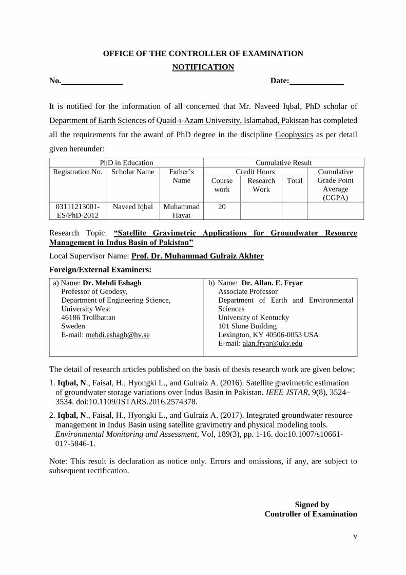
It is notified for the information of all concerned that Mr. Naveed Iqbal, PhD scholar of
Department of Earth Sciences of Quaid-i-Azam University, Islamabad, Pakistan has completed
all the requirements for the award of PhD degree in the discipline Geophysics as per detail
given hereunder:
PhD in Education Cumulative Result
Registration No. Scholar Name Father’s
Name
Credit Hours Cumulative
Grade Point
Average
(CGPA)
Course
work
Research
Work
Total
03111213001-
ES/PhD-2012
Naveed Iqbal Muhammad
Hayat
20
Research Topic: “Satellite Gravimetric Applications for Groundwater Resource
Management in Indus Basin of Pakistan”
Local Supervisor Name: Prof. Dr. Muhammad Gulraiz Akhter
Foreign/External Examiners:
a) Name: Dr. Mehdi Eshagh
Professor of Geodesy,
Department of Engineering Science,
University West
46186 Trollhattan
Sweden
E-mail: [email protected]
b) Name: Dr. Allan. E. Fryar
Associate Professor
Department of Earth and Environmental
Sciences
University of Kentucky
101 Slone Building
Lexington, KY 40506-0053 USA
E-mail: [email protected]
The detail of research articles published on the basis of thesis research work are given below;
1. Iqbal, N., Faisal, H., Hyongki L., and Gulraiz A. (2016). Satellite gravimetric estimation
of groundwater storage variations over Indus Basin in Pakistan. IEEE JSTAR, 9(8), 3524–
3534. doi:10.1109/JSTARS.2016.2574378.
2. Iqbal, N., Faisal, H., Hyongki L., and Gulraiz A. (2017). Integrated groundwater resource
management in Indus Basin using satellite gravimetry and physical modeling tools.
Environmental Monitoring and Assessment, Vol, 189(3), pp. 1-16. doi:10.1007/s10661-
017-5846-1.
Note: This result is declaration as notice only. Errors and omissions, if any, are subject to
subsequent rectification.
Signed by
Controller of Examination
vi
DEDICATION
Dedicated to my beloved Wife and Daughter whose unforgettable
sacrifice and unconditional support, motivated me to complete my PhD
vii
ACKNOWLEDGEMENTS
All praises are to Almighty Allah, the most merciful and the most beneficent, Who
created the universe for the human beings, and offered them to explore his master piece the
earth and to see the signs of his powerfulness. I am thankful to my ALLAH Who has blessed
me with courage and strength for the accomplishment of this thesis. Secondly, praises are for
the last and beloved Prophet Muhammad (Peace Be Upon Him) who is a continuous source of
guidance for mankind towards the righteous path.
I am very grateful to my respected supervisor, Prof. Dr. Muhammad Gulraiz Akhter for
his guidance, encouragement and inspiration, which has finally resulted in the compilation of
my dissertation. His continuous cooperation and encouragement provided me motivation to
accomplish my PhD.
I would like to express my immense gratitude to Dr. A. D. Khan, Ex-Director General,
Pakistan Council of Research in Water Resources (PCRWR) for his professional guidance. It
would not be the justice if I could not acknowledge the technical and financial supported
extended by Dr. Faisal Hossain, University of Washington, USA. His unconditional support
and enthusiasm provided me an opportunity to complete my research work well in time. I am
also thankful to Dr. Muhammad Ashraf, Chairman (PCRWR) for his encouragement to find
some economical and practically viable solution of the complex problem related to
groundwater resource management.
Scarp Monitoring Organization (SMO), WAPDA, Lahore, Punjab Irrigation
Department, Lahore, Pakistan Meteorological Department (PMD), Islamabad are greatly
acknowledged for the provision of related datasets. Finally, I wish to express my deepest
gratitude to my mother and brothers especially Muzaffar Iqbal (late), for their prayers,
encouragement and moral support during my studies. I am also pleased to extend my sincere
thanks to all my friends and colleagues specially Dr. Hammad Gilani and Dr. Waqas A. Qazi
for their well wishes and professional support for my success.
Naveed Iqbal
viii
ABSTRACT
The goal of this study is accurate quantification of groundwater storage changes for
effective groundwater resource management in Indus Basin of Pakistan. This study uses
satellite integrated physical modeling methodology to analyze the groundwater dynamics over
Upper Indus Plain (UIP), which covers Punjab Province of Pakistan. The GRACE (Gravity
Recovery and Climate Experiment) data has been used for the extraction of Terrestrial Water
Storage (TWS) changes and then Variable Infiltration Capacity (VIC) Model has been applied
to derive Groundwater Storage (GWS) changes from 2003-2010. The VIC model has been
specifically developed for Indus Basin at 0.1˚ × 0.1˚ grid scale to simulate daily soil moisture
and surface water fluxes. The evenly distributed ground observation data of about 150
piezometric water level changes has been used for the calibration (2003-2007) and validation
(2008-2010) purposes. In comparison with Indus Basin of Pakistan (IBP), the results suggest
that UIP is at the wave of more rapid variations both in terms of total water storage as well as
groundwater storage anomalies due to over exploitation of groundwater for anthropogenic
purposes. The intensity of these variations in terms of decrease either in TWS or GWS over
UIP is about three times higher than IBP. While investigation and analysis, it is estimated that
UIP has lost a stock of about 11.84 km3 of fresh groundwater storage in just 8 years of time
(2003-2010) through extensive groundwater abstraction. The projected scenario (2011-2014)
indicate further loss of fresh groundwater storage due to increasing dependence on
groundwater.
The potential of GRACE derived methodology has been evaluated at effective
groundwater management scales (doabs) using numerical downscaling technique. The
accuracy of GRACE derived GWS has been evaluated at each doab (the area bounded by two
rivers) scale and the phenomenon of groundwater depletion and recharge have been quantified.
The seasonal to annual changes have been analyzed to study the groundwater system behavior,
flooding impact and critical areas have been identified where; groundwater sustainability is at
risk. While studying the groundwater dynamics at local scales, the detailed investigation
reveals that GRCAE is more effective when the study area is comparable enough to the spatial
resolution of GRACE or the trends of groundwater recharge and depletion are significantly
persistent. Resultantly, GRACE has found more successful in two (Bari and Rechna doabs) out
of four doabs where groundwater depletion trends (depletion or recharge) are more prominent
and persistent enough. Subsequently, the vulnerability of groundwater sustainability is at the
verge of moderate to severe in Rechna and Bari doabs respectively. It is estimated that GWS
ix
has depleted at the rate of 0.38 km3/year in Bari and 0.21 km3/year in Rechna doabs over the
period 2003-2010. It is observed that the areas of Lower Bari (Multan, Lodhran, Khanewal
including Lahore) and some parts of Rechna doabs (Toba Tek Singh and parts of the Jhang
districts) are under stress where the excessive pumping dominates the recharge. Therefore,
immediate attention is required by the concerned departments with some remedial measures.
The designed methodology has been compared and found in good agreement with the
traditional approaches like piezometric monitoring and groundwater modeling in terms of
trends. Being an underground resource with dynamic nature, the integrated methodology
consisting of the GRACE, VMOD and piezometric monitoring is suggested quite useful, which
would help improve the accurate quantification of abstraction and recharge mechanisms. This
would impact the competency to plan effective management strategies. The evaluation of
statistical approach for future projection resulted an average standard error (SE) of 9 mm and
7 mm in Bari and Rechna doabs respectively with favorable correlation and found suitably
appropriate for 3-6 monthly future projection. However, this technique is not found appropriate
for Chaj and Bari doabs due to disagreement with Piezo-GWS over the calibration period.
The study also outlines the potential opportunities and challenges associated with
satellite gravimetric applications for operational groundwater management. This study has also
suggested appropriate management strategies to ensure the aquifer sustainability of Indus
Basin.
x
Table of Contents
CHAPTER 1 ............................................................................................................................. 1
INTRODUCTION.................................................................................................................... 1
1.1 BACKGROUND ................................................................................................................. 1
1.2 STUDY AREA .................................................................................................................. 2
1.3 HYDROLOGY ................................................................................................................... 6
1.4 LITERATURE REVIEW .................................................................................................... 16
1.5 PROBLEM STATEMENT .................................................................................................. 22
1.6 OBJECTIVES .................................................................................................................. 22
CHAPTER 2 ........................................................................................................................... 23
DATASETS AND METHODOLOGY ................................................................................. 23
2.1 GRACE DATASETS ...................................................................................................... 23
2.2 PIEZOMETRIC DATASETS............................................................................................... 24
2.3 VARIABLE INFILTRATION CAPACITY (VIC) MODEL DATASETS .................................... 24
2.4 METHODOLOGY ............................................................................................................ 25
CHAPTER 3 ........................................................................................................................... 29
GRACE DATA PROCESSING AND HYDROLOGICAL MODELING ........................ 29
3.1 RELATION BETWEEN SURFACE MASS AND GRAVITY .................................................... 29
3.2 PROCESSING OF SPHERICAL HARMONIC COEFFICIENTS ................................................ 32
3.2.1 Step-0: Rename Data Files................................................................................... 32
3.2.2 Step-1: Extract SHCs ........................................................................................... 33
3.2.3 Step-2 & 3: Geocentre & Truncation ................................................................... 34
3.2.4 Step-4 & 5: Average Calculation and Reference Subtraction ............................. 34
3.2.5 Step-6 & 7: Remove PGR and Decorrelation Filter ............................................ 35
3.2.6 Step-8 & 9: Transform SHCs to Mass and Mass to Grids ................................... 35
3.2.7 Step-10: Gaussian Smoothing and Leakage Reduction ....................................... 36
3.3 SIGNAL RESTORATION .................................................................................................. 36
3.4 VARIABLE INFILTRATION CAPACITY MODEL (VIC)...................................................... 37
3.4.1 VIC Model Simulation and Calibration ............................................................... 38
CHAPTER 4 ........................................................................................................................... 45
ESTIMATION OF GWS VARIATIONS OVER INDUS BASIN ..................................... 45
4.1 TOTAL WATER STORAGE VARIATIONS ......................................................................... 45
4.2 GROUNDWATER STORAGE VARIATIONS........................................................................ 46
4.3 GWS CALIBRATION ANALYSIS ..................................................................................... 48
4.4 FLOODING ANALYSIS .................................................................................................... 52
CHAPTER 5 ........................................................................................................................... 54
INTEGRATION OF SATELLITE GRAVIMETRY WITH PHYSICAL MODELING
TOOLS .................................................................................................................................... 54
5.1 GROUNDWATER MONITORING THROUGH GROUND OBSERVATIONAL NETWORK .......... 54
5.2 GROUNDWATER MODELING .......................................................................................... 57
5.3 SATELLITE GWS DOAB SCALE ESTIMATION ................................................................ 60
5.4 INTEGRATED GROUNDWATER MANAGEMENT ............................................................... 67
xi
5.5 GRACE – A SPATIAL DECISION SUPPORT TOOL .......................................................... 83
5.6 TRACKING GROUNDWATER FROM SPACE ...................................................................... 84
5.6.1 Opportunities........................................................................................................ 84
5.6.2 Challenges ............................................................................................................ 84
CHAPTER 6 ........................................................................................................................... 86
CONCLUSION AND RECOMMENDATIONS ................................................................. 86
6.1 CONCLUSIONS ............................................................................................................... 86
6.2 RECOMMENDATIONS ..................................................................................................... 88
REFERENCES ....................................................................................................................... 90
LIST OF PUBLICATIONS .................................................................................................. 95
SEMINAR PRESENTATIONS ............................................................................................ 95
CONFERENCE AND WORKSHOP PARTICIPATION ................................................. 95
REPRINTS OF PUBLICATIONS ....................................................................................... 97
APPENDIX ............................................................................................................................. 99
APPENDIX-A: EXAMPLES OF MODEL BUILDER TOOL FOR DATA PROCESSING AND ANALYSIS
IN ARC GIS SOFTWARE ......................................................................................................... 99
APPENDIX-B: VIC SIMULATION RESULTS OVER INDUS BASIN (2002-2010) ........................ 99
APPENDIX-C: OBSERVED ANNUAL RIVER INFLOWS (MAF) ............................................... 100
APPENDIX-D: ESTIMATION OF GROUNDWATER STORAGE VARIATIONS DERIVED FROM
GLDAS AND VIC ............................................................................................................... 101
APPENDIX-E: CALCULATION PROCEDURE FOR GROUNDWATER STORAGE ANOMALIES ..... 104
xii
LIST OF FIGURES
Figure 1.1: Location map of study area. AJK stands for Azad Jammu and Kashmir. ............... 3
Figure 1.2: Topographic variations over UIP. The contours (purple color) are derived from
SRTM 90 meter USGS-DEM with 5-meter interval. AJK stands for Azad Kashmir. .............. 5
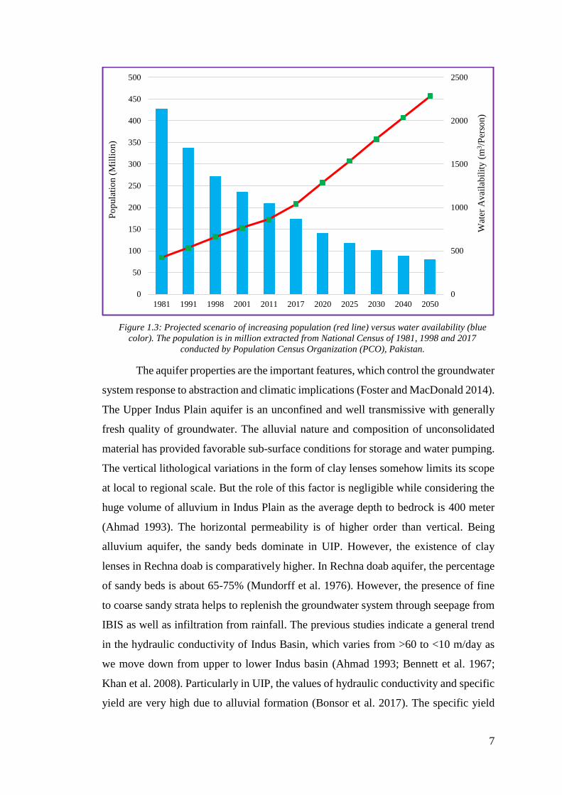
Figure 1.3: Projected scenario of increasing population (red line) versus water availability (blue
color). The population is in million extracted from National Census of 1981, 1998 and 2017
conducted by Population Census Organization (PCO), Pakistan. ............................................. 7
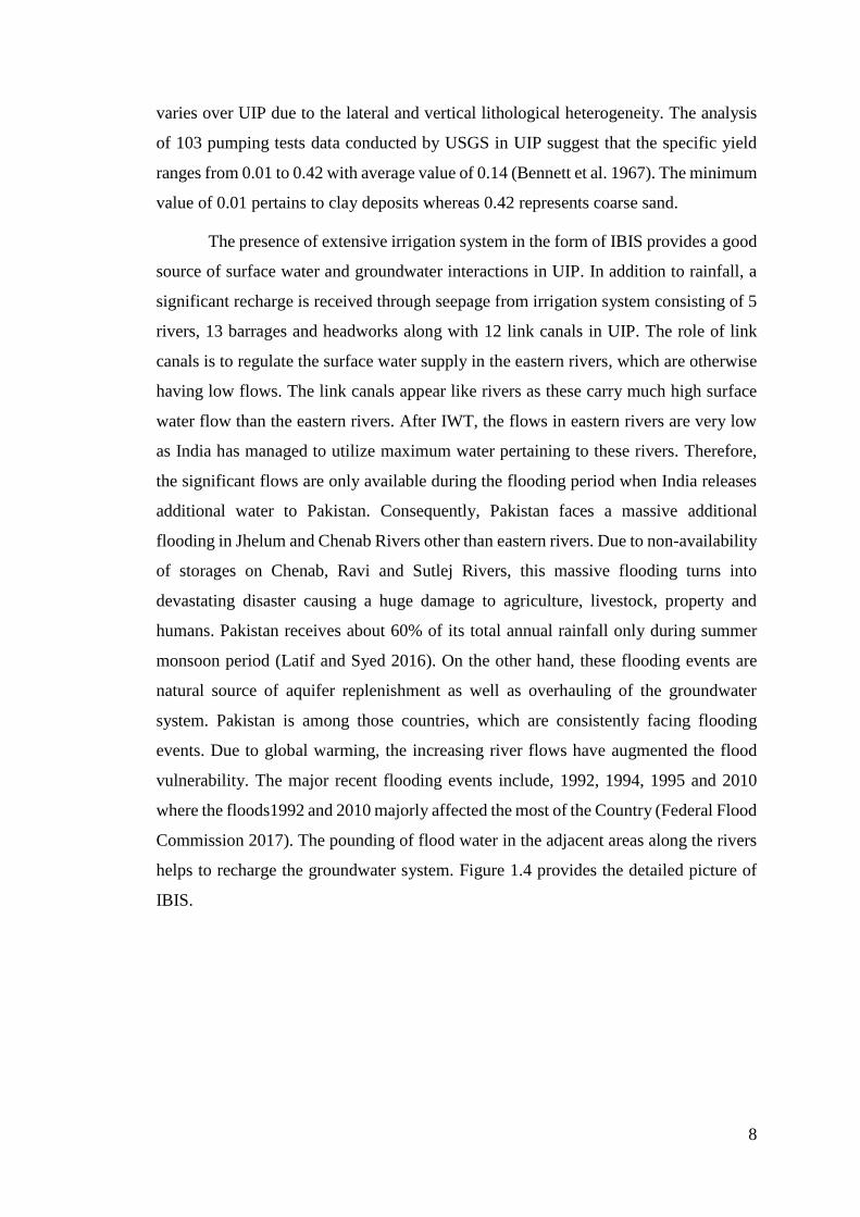
Figure 1.4: Indus Basin Irrigation System (IBIS) in UIP. The irrigation system (river and
canals) are in blue color whereas, the red dots are the locations of barrages. ........................... 9
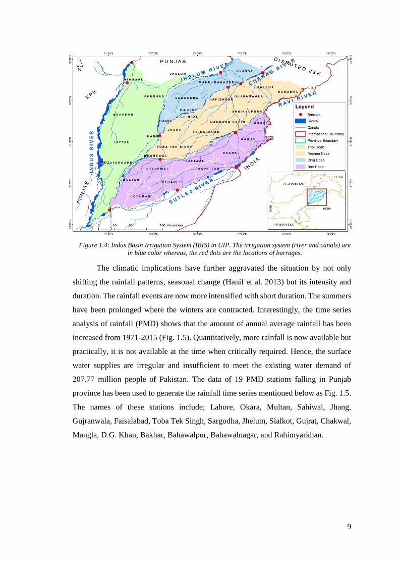
Figure 1.5: Annual average rainfall variations from 1971-2015 in Punjab Province. The blue
lines is the rainfall time series generated using PMD station data. The dotted line in red color
shows the overall rainfall trend. ............................................................................................... 10
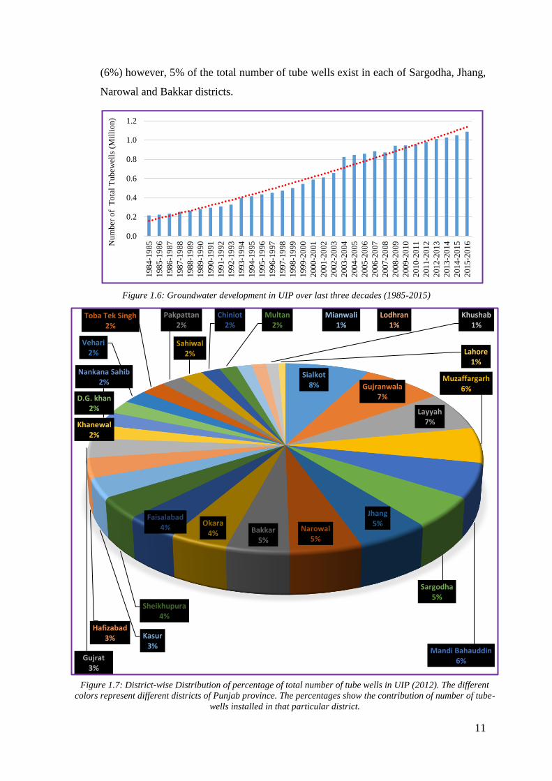
Figure 1.6: Groundwater development in UIP over last three decades (1985-2015) .............. 11
Figure 1.7: District-wise Distribution of percentage of total number of tube wells in UIP (2012).
The different colors represent different districts of Punjab province. The percentages show the
contribution of number of tube-wells installed in that particular district. ............................... 11
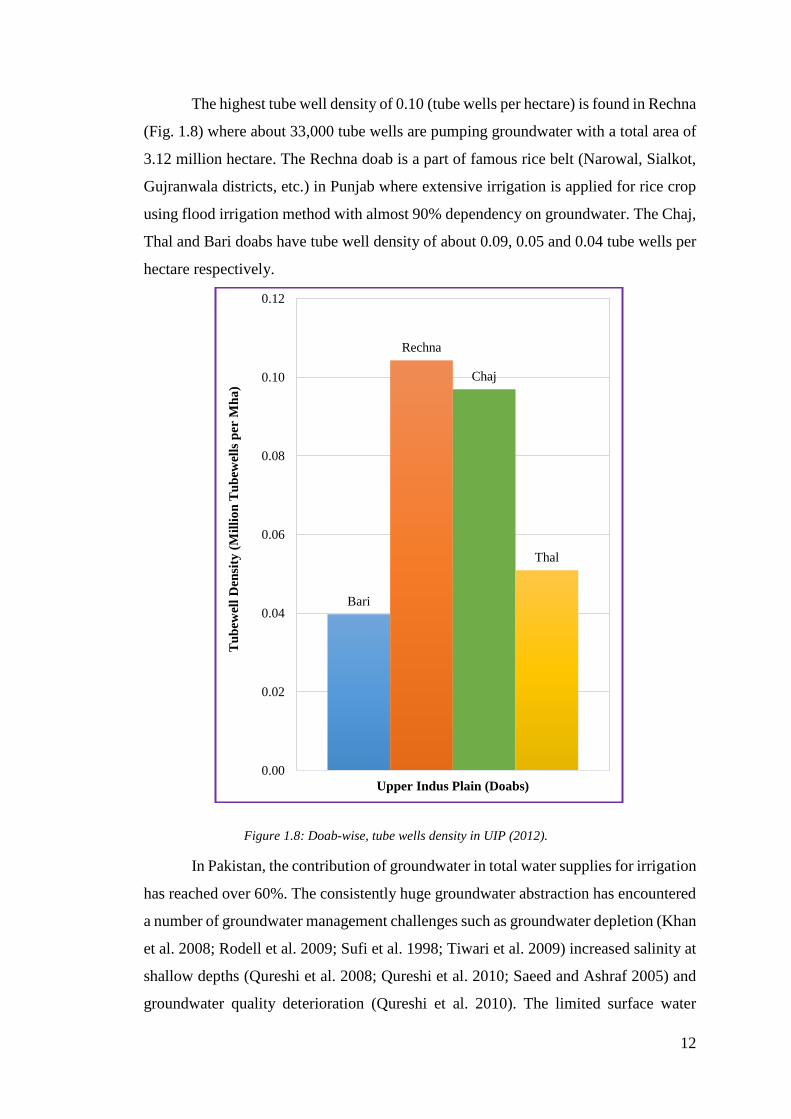
Figure 1.8: Doab-wise, tube wells density in UIP (2012)........................................................ 12
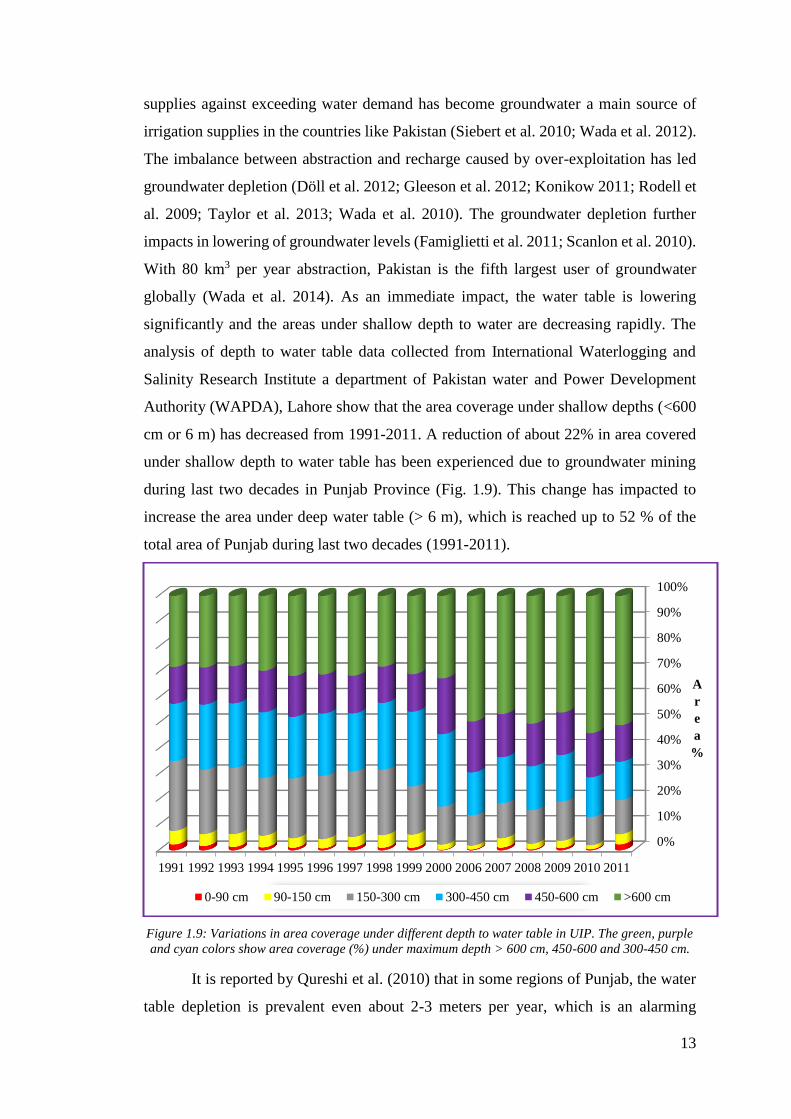
Figure 1.9: Variations in area coverage under different depth to water table in UIP. The green,
purple and cyan colors show area coverage (%) under maximum depth > 600 cm, 450-600 and
300-450 cm. ............................................................................................................................. 13
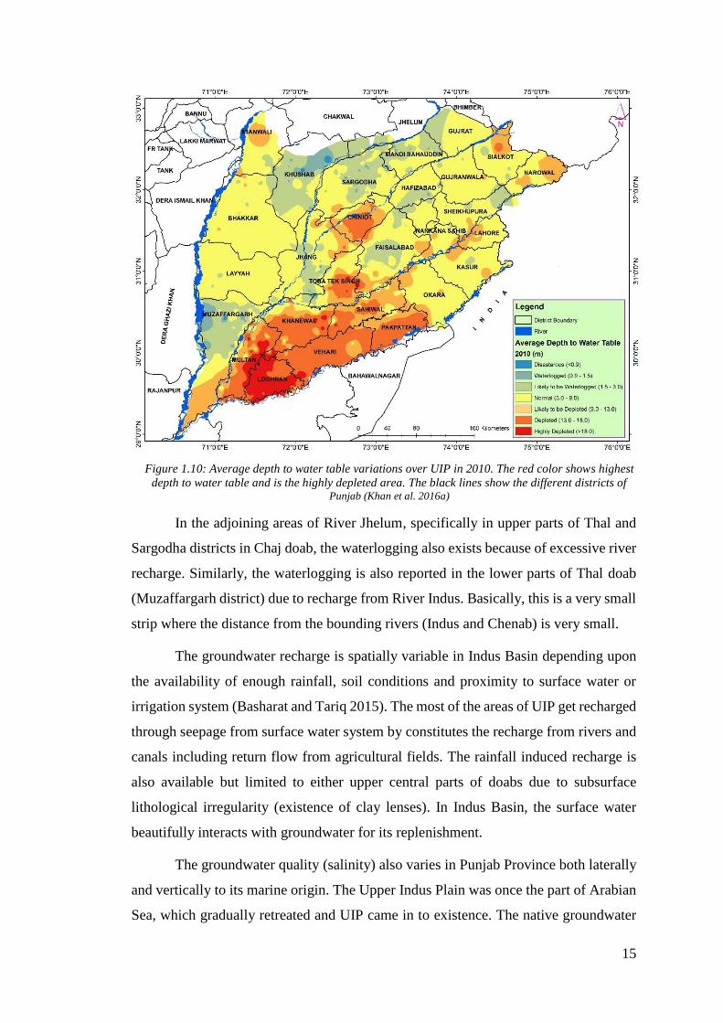
Figure 1.10: Average depth to water table variations over UIP in 2010. The red color shows
highest depth to water table and is the highly depleted area. The black lines show the different
districts of Punjab (Khan et al. 2016a)..................................................................................... 15
Figure 2.1: GRACE mission data flow describes the process of data collection and different
data processing levels (adopted from http://www.csr.utexas.edu/grace/) ................................ 23
Figure 2.2: Flow chart methodology for the estimation of groundwater storage anomaly ...... 26
Figure 3.1: Step by step methodological approach for the GRACE data processing .............. 32
Figure 3.2: Calibration stations, the numbers are the normalized RMSE at each station. The
Indus ......................................................................................................................................... 40
Figure 3.3: Variations of SMR anomalies during February 2003 over Indus Basin (0.1˚ × 0.1˚)
.................................................................................................................................................. 43
Figure 3.4: Variations of average SMR anomalies (2003-2010) over Indus Basin (1˚ × 1˚). . 43
Figure 3.5: Variations of average SMR anomalies (2003-2010) over UIP (0.1˚× 0.1˚) .......... 44
Figure 4.1: Mean trend map of TWS anomalies from 2003-2010 over Indus Basin. The red
color represents highest depletion in total water storage followed by yellowish, light green and
cyan colors ............................................................................................................................... 45
Figure 4.2: Comparison of TWS, GWS and SM from 2003-2010 over UIP........................... 46
Figure 4.3: Comparison of VIC based GRACE-GWS changes (blue) with GLDAS-1 based
GRACE-GWS changes (yellow) ............................................................................................. 48
xiii
Figure 4.4: Comparison of GRACE-GWS (red color) anomalies with piezometric-GWS (blue
color) over UIP (2003-2010) ................................................................................................... 48
Figure 4.5 Groundwater stock variations over UIP from 2003-2014 ...................................... 52
Figure 5.1: Piezometric network of water level monitoring in UIP. The reddish dots are the
water table measurement locations used for calibration purpose ............................................ 54
Figure 5.2: Variations in average depth to water table over UIP in 2010. .............................. 56
Figure 5.3: Average depth to water table variations in Lodhran, Multan and Khanewal from
2005-2010. LMK (yellow bar) is annual average trend of groundwater depletion in three
districts. .................................................................................................................................... 57
Figure 5.4: Doab scale annual average variations in groundwater simulated with Visual
ModFlow over UIP from 2000-2010 ....................................................................................... 58
Figure 5.5: ModFlow simulated annual average variations in groundwater over Bari and
Rechna doabs from 2000-2010 ................................................................................................ 59
Figure 5.6: ModFlow simulated annual average variations in groundwater over Chaj doab from
2000-2010 ................................................................................................................................ 59
Figure 5.7: ModFlow simulated annual average variations in groundwater over Thal doab from
2000-2010 ................................................................................................................................ 59
Figure 5.8: Annual average groundwater storage variations in 2003 over UIP. Dark red color
shows negative change representing depletion in groundwater storage .................................. 61
Figure 5.9: Annual average groundwater storage variations in 2004 over UIP....................... 62
Figure 5.10: Annual average groundwater storage variations in 2005 over UIP ..................... 62
Figure 5.11: Annual average groundwater storage variations in 2006 over UIP ..................... 63
Figure 5.12: Annual average groundwater storage variations in 2007 over UIP ..................... 63
Figure 5.13: Annual average groundwater storage variations in 2008 over UIP ..................... 64
Figure 5.14: Annual average groundwater storage variations in 2009 over UIP ..................... 64
Figure 5.15: Annual average groundwater storage variations in 2010 over UIP ..................... 65
Figure 5.16: Annual average groundwater storage variations from 2003-2009 over UIP ....... 65
Figure 5.17: Annual average groundwater storage variations from 2003-2010 over UIP ....... 66
Figure 5.18: Change in groundwater storage from July-August, 2010 over UIP .................... 66
Figure 5.19: Comparison of the GRACE along with Piezometric derived variations in
groundwater storage over Bari doab from 2003-2010 ............................................................. 69
Figure 5.20: Comparison of the GRACE along with Piezometric derived variations in
groundwater storage over Rechna doab from 2003-2010 ........................................................ 69
Figure 5.21: Seasonal changes in groundwater stock over Bari doab from 2003-2010 .......... 72
Figure 5.22: Seasonal changes in groundwater stock over Rechna doab from 2003-2010 ..... 72
Figure 5.23: Comparison of the GRACE along with Piezometric derived variations in
groundwater storage over Chaj doab from 2003-2010 ............................................................ 73
Figure 5.24: Comparison of the GRACE along with Piezometric derived variations in
groundwater storage over Thal doab from 2003-2010 ............................................................ 73
xiv
Figure 5.25: Seasonal changes in groundwater stock over Chaj doab from 2003-2010.......... 76
Figure 5.26: Seasonal changes in groundwater stock over Thal doab from 2003-2010 .......... 76
Figure 5.27: Correlation between the GRACE and piezometric groundwater storage variations
over Bari doab during calibration period (2003-2007) ............................................................ 78
Figure 5.28: Variations in standard error over Bari doab during projected period (January-June,
2011) ........................................................................................................................................ 78
Figure 5.29: Correlation between the GRACE and piezometric groundwater storage variations
over Rechna doab during calibration period (2003-2007) ....................................................... 79
Figure 5.30: Variations in standard error over Rechna doab during projected period (January-
June, 2011) ............................................................................................................................... 79
Figure 5.31: Correlation between the GRACE and piezometric groundwater storage variations
over Chaj doab during calibration period (2003-2007) ........................................................... 80
Figure 5.32: Variations in standard error over Chaj doab during projected period (January-June,
2011) ........................................................................................................................................ 80
Figure 5.33: Correlation between the GRACE and piezometric groundwater storage variations
over Thal doab during calibration period (2003-2007) ............................................................ 81
Figure 5.34: Variations in standard error over Thal doab during projected period (January-June,
2011) ........................................................................................................................................ 81
xv
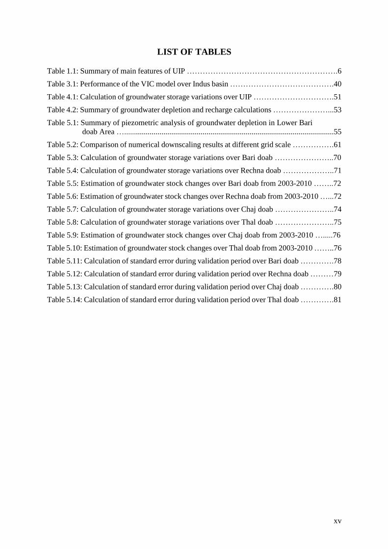
LIST OF TABLES Table 1.1: Summary of main features of UIP ………………………………………………….6
Table 3.1: Performance of the VIC model over Indus basin ………………………………….40
Table 4.1: Calculation of groundwater storage variations over UIP ………………………….51
Table 4.2: Summary of groundwater depletion and recharge calculations …………………...53
Table 5.1: Summary of piezometric analysis of groundwater depletion in Lower Bari
doab Area …...........................................................................................................55
Table 5.2: Comparison of numerical downscaling results at different grid scale …………….61
Table 5.3: Calculation of groundwater storage variations over Bari doab …………………..70
Table 5.4: Calculation of groundwater storage variations over Rechna doab ………………..71
Table 5.5: Estimation of groundwater stock changes over Bari doab from 2003-2010 ……..72
Table 5.6: Estimation of groundwater stock changes over Rechna doab from 2003-2010 …...72
Table 5.7: Calculation of groundwater storage variations over Chaj doab …………………..74
Table 5.8: Calculation of groundwater storage variations over Thal doab …………………..75
Table 5.9: Estimation of groundwater stock changes over Chaj doab from 2003-2010 ….....76
Table 5.10: Estimation of groundwater stock changes over Thal doab from 2003-2010 ……..76
Table 5.11: Calculation of standard error during validation period over Bari doab ………….78
Table 5.12: Calculation of standard error during validation period over Rechna doab ………79
Table 5.13: Calculation of standard error during validation period over Chaj doab ………….80
Table 5.14: Calculation of standard error during validation period over Thal doab ………….81
xvi
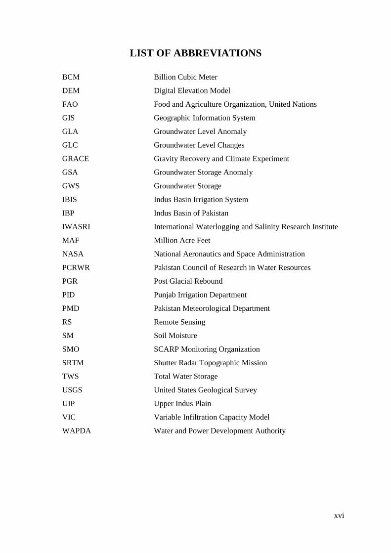
LIST OF ABBREVIATIONS
BCM Billion Cubic Meter
DEM Digital Elevation Model
FAO Food and Agriculture Organization, United Nations
GIS Geographic Information System
GLA Groundwater Level Anomaly
GLC Groundwater Level Changes
GRACE Gravity Recovery and Climate Experiment
GSA Groundwater Storage Anomaly
GWS Groundwater Storage
IBIS Indus Basin Irrigation System
IBP Indus Basin of Pakistan
IWASRI International Waterlogging and Salinity Research Institute
MAF Million Acre Feet
NASA National Aeronautics and Space Administration
PCRWR Pakistan Council of Research in Water Resources
PGR Post Glacial Rebound
PID Punjab Irrigation Department
PMD Pakistan Meteorological Department
RS Remote Sensing
SM Soil Moisture
SMO SCARP Monitoring Organization
SRTM Shutter Radar Topographic Mission
TWS Total Water Storage
USGS United States Geological Survey
UIP Upper Indus Plain
VIC Variable Infiltration Capacity Model
WAPDA Water and Power Development Authority
1
CHAPTER 1
Introduction
1.1 Background
Groundwater is a finite, dependable and life sustained resource. It is also a
renewable underground resource and an important component of hydrological cycle.
The aquifers help to ensure constant water supply throughout the year where, the
surface water supplies are inconsistent. The Indus Basin is one of the large basins of
the world and Pakistan is one of the countries who share this transboundary basin (Long
et al. 2014). In Pakistan, the groundwater has emerged as a main source to meet about
90% drinking water requirements and more than 60% irrigation water supplies are also
supplemented through groundwater (Cheema et al. 2014). The agriculture sector is
called the backbone of the country. It is not only contributing about 21% in GDP, but
also providing about 24% employment opportunities in the rural areas (Qureshi et al.
2003). Increasing population, inadequate storage capacity, inconsistent surface water
supplies, ineffective water management, traditional irrigation practices and climatic
variability has increased the dependence on groundwater. The abundance of fresh
groundwater availability and lack of groundwater regulation has further hampered the
groundwater sustainability. Thus, the farmers have the liberty to drill tube wells
anywhere and pump any quantity of groundwater. Consequently, the number of private
tube wells has exponentially increased over time. More than one million tube wells
(public & private) are pumping fresh groundwater in Upper Indus Plain – Punjab
Province (Bureau of Statistics 2012). As a result of unsustainable use of groundwater,
the water table is depleting along with groundwater quality deterioration (Qureshi et al.
2008; Qureshi et al. 2010). In Upper Indus Plain, some areas are under physical
groundwater mining due to imbalance between recharge and pumping. Under such
situation, the long-term agricultural productivity is directly linked with the
sustainability of groundwater aquifer.
The effective groundwater management requires accurate assessment of
recharge and discharge processes. For this purpose, the availability of frequent and
reliable information pertaining to groundwater behavior, utilization patterns and its
response to climatic implications, helps to devise better management strategies. Being
an underground resource, the estimation of such groundwater parameters becomes
challenging due to system complexities and dynamic nature of Indus Basin.
2
Additionally, the provision of such type of detailed information in spatio-temporal
domains is generally not available in developing countries like Pakistan. The
insufficient and sporadic ground monitoring networks, data sharing issues, week
institutional capacities and professional skills are the key challenges for groundwater
management. These challenges have not only hampered the efforts of national to basin-
wide groundwater budgeting but also limit the scope of traditional tools and methods
in space and time. In the context of Pakistan, the groundwater regulation requires
systematic monitoring mechanism for successful implementation, which is presently
not in place. Thus, the prevailing situation emphasizes the need for the exploration of
potential alternate technologies to bridge information gaps in spatio-temporal domains.
1.2 Study Area
Indus is a trans-boundary basin with total area of 1,143,000 km2 (Long et al.
2014) shared by Pakistan, India, China and Afghanistan. With 60% basin area coverage
in Pakistan, Indus Basin is playing major role by meeting irrigation requirements and
considered as backbone of the agriculture-based economy of Pakistan. Originating from
Tibetan Plateau, Indus River passes through high mountains in the north and then meets
the Arabian Sea by making its way through Indus Plain. The mighty Indus along with
its five tributaries (Kabul, Jhelum, Chenab, Ravi and Sutlej) irrigates the fertile land of
Punjab and Sindh Provinces to meet most of the food and fiber requirements of the
Country. The Upper Indus Plain (UIP) consisting of major part of Punjab Province is
blessed with plenty of fresh groundwater resource in the form of unconfined aquifer.
Being sandy in nature, the aquifer gets replenishment through seepage from Indus Basin
Irrigation System (IBIS) as well as infiltration from rainwater. The IBIS is more than a
half century’s old system of irrigation, which was developed after Indus Water Treaty
(IWT) in 1960. The IWT was signed between Pakistan and India by allocating the water
rights of western rivers (Indus, Jhelum and Chenab) to Pakistan whereas; the three
eastern rivers (Ravi, Sutlej and Bias) were given to India. In the eastern rivers, India
only releases surplus water mostly in monsoon (July-September) period whereas these
rivers remain dry for most of the period and flow like drains. To maintain the water
supplies in the eastern rivers, Pakistan has developed an interconnected system of
irrigation canals called as IBIS. The main objective of this IBIS was to maintain the
water supplies in the eastern rivers by diverting the additional water from western rivers
through a network of link canals. For this purpose, various structures like barrages and
3
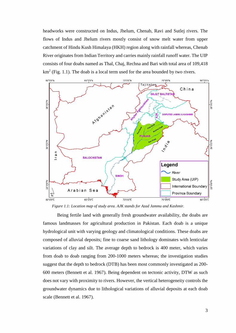
headworks were constructed on Indus, Jhelum, Chenab, Ravi and Sutlej rivers. The
flows of Indus and Jhelum rivers mostly consist of snow melt water from upper
catchment of Hindu Kush Himalaya (HKH) region along with rainfall whereas, Chenab
River originates from Indian Territory and carries mainly rainfall runoff water. The UIP
consists of four doabs named as Thal, Chaj, Rechna and Bari with total area of 109,418
km2 (Fig. 1.1). The doab is a local term used for the area bounded by two rivers.
Figure 1.1: Location map of study area. AJK stands for Azad Jammu and Kashmir.
Being fertile land with generally fresh groundwater availability, the doabs are
famous landmasses for agricultural production in Pakistan. Each doab is a unique
hydrological unit with varying geology and climatological conditions. These doabs are
composed of alluvial deposits; fine to coarse sand lithology dominates with lenticular
variations of clay and silt. The average depth to bedrock is 400 meter, which varies
from doab to doab ranging from 200-1000 meters whereas; the investigation studies
suggest that the depth to bedrock (DTB) has been most commonly investigated as 200-
600 meters (Bennett et al. 1967). Being dependent on tectonic activity, DTW as such
does not vary with proximity to rivers. However, the vertical heterogeneity controls the
groundwater dynamics due to lithological variations of alluvial deposits at each doab
scale (Bennett et al. 1967).
4
The geology of Thal doab is composed of unconsolidated quaternary alluvial
and aeolian deposits. A thick layer of the alluvial material is underlain by basement
rocks. These basement rocks are as old as Precambrian. The Salt Range covers one side
of upper part of Thal doab and consists of highly fractured, folded and fossiliferous
rocks of Cambrian to Pleistocene age (Bennett et al. 1967). The piedmont alluvial
deposits are found near the foothills of Salt Range whereas the central part of Thal doab
is covered with extensive surficial aeolian sand deposit. In Chaj and Rechna doabs, the
quaternary alluvium deposition is of Precambrian age, which extends on semi-
consolidated tertiary rocks. The northern part of Chaj doab is covered by Pabbi Hills,
which is a range belonging to the Himalayan foothills. Its upper part belongs to Siwalik
System with Tertiary age (Greenman et al. 1967). The Siwalik rocks form the lower
and outermost hills of the Himalayan mountain ranges with middle Miocene to early
Pleistocene age. The Kirana hills forms the oldest rocks in Rechna doab having
Precambrian age. Basically, Kirrana hills are a group of rocks found in the areas of
Sangla, Chiniot and Shah Kot. The geology of Bari doab is very much similar to Rechna
doab. The flood plains abandoned flood plains and bar upland are three dominant
physiographic features of Bari doab. The flood plain area is locally known as “Sailaba”.
It is a narrow strip of about 2-8 miles wide. The abandoned flood plains is the dominant
unit as it covers about two third area whereas the Bar Uplands forms the central part of
Bari doab.
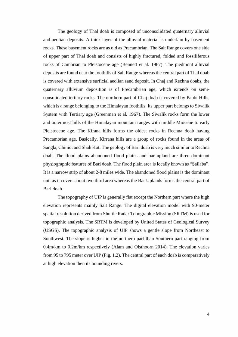
The topography of UIP is generally flat except the Northern part where the high
elevation represents mainly Salt Range. The digital elevation model with 90-meter
spatial resolution derived from Shuttle Radar Topographic Mission (SRTM) is used for
topographic analysis. The SRTM is developed by United States of Geological Survey
(USGS). The topographic analysis of UIP shows a gentle slope from Northeast to
Southwest. The slope is higher in the northern part than Southern part ranging from
0.4m/km to 0.2m/km respectively (Alam and Olsthoorn 2014). The elevation varies
from 95 to 795 meter over UIP (Fig. 1.2). The central part of each doab is comparatively
at high elevation then its bounding rivers.
5
Figure 1.2: Topographic variations over UIP. The contours (purple color) are derived from SRTM 90
meter USGS-DEM with 5-meter interval. AJK stands for Azad Kashmir.
The UIP is densely populated area with extensive agricultural activities. Wheat,
Rice, Sugarcane, Cotton and some other cash crops (pulses, vegetables, etc.) are the
major crops. The climate of UIP varies from semi-humid to arid. The summers are very
hot (> 45 C˚) whereas the temperature during winter seasons remains around 20 C˚. The
rainfall is very erratic and mostly received during monsoon period, which prevails from
July to September. The last forty years meteorological records indicate that annual
average rainfall over Punjab Province is 580 mm (Ahmad et al. 2014). The Chaj
followed by Rechna and Thal doabs receive maximum rainfall whereas, the annual
average rainfall in Bari doab is reported to be the least (varies from 100-500 mm)
(Ahmad et al. 2014). The major characteristics of UIP are summarized in Table 1.1.
6
1.3 Hydrology
In 1950, the surface water was adequate to meet the irrigation demand in
Pakistan with 5000 m3 per capita water availability, which has been decreased to <1000
m3 (Yu et al. 2013) due to increasing water demand caused by exponential population
growth. Over the time, the water demand has increased whereas the total water
availability remained the same. Under such situation, Pakistan is enlisted among water
scarce or water insecure countries. According to Falkenmark et al. (2007), any country
having <1000 m3 per capita water availability falls under the category of water insecure
countries. The reduced storage capacity of existing reservoirs due to siltation and
dramatic increasing in population of 207.77 million people has resulted imbalance
between demand and total water availability. The projected water scenarios show that
the situation will be worst in future if the storage enhancement remains at the same pace
(Fig. 1.3). Despite of the clear need, the lack of political consensus among provinces
and financial constraints are the major hindrance in the construction of medium to mega
dams such as Bhasha and Kalabagh. Additionally, the climatic implications such as
devastating flooding events has further aggravated the situation with variable surface
water supplies. Resultantly, the pressure on groundwater has gradually increased to
meet the deficit in overall water supplies.
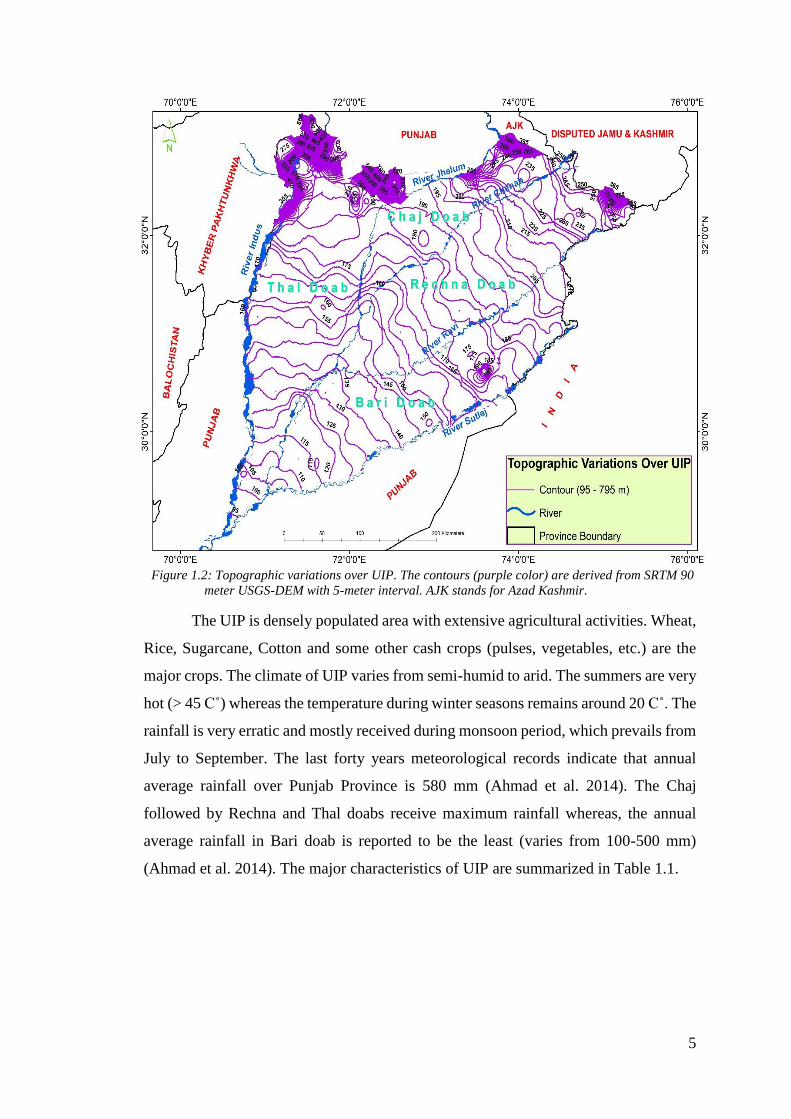
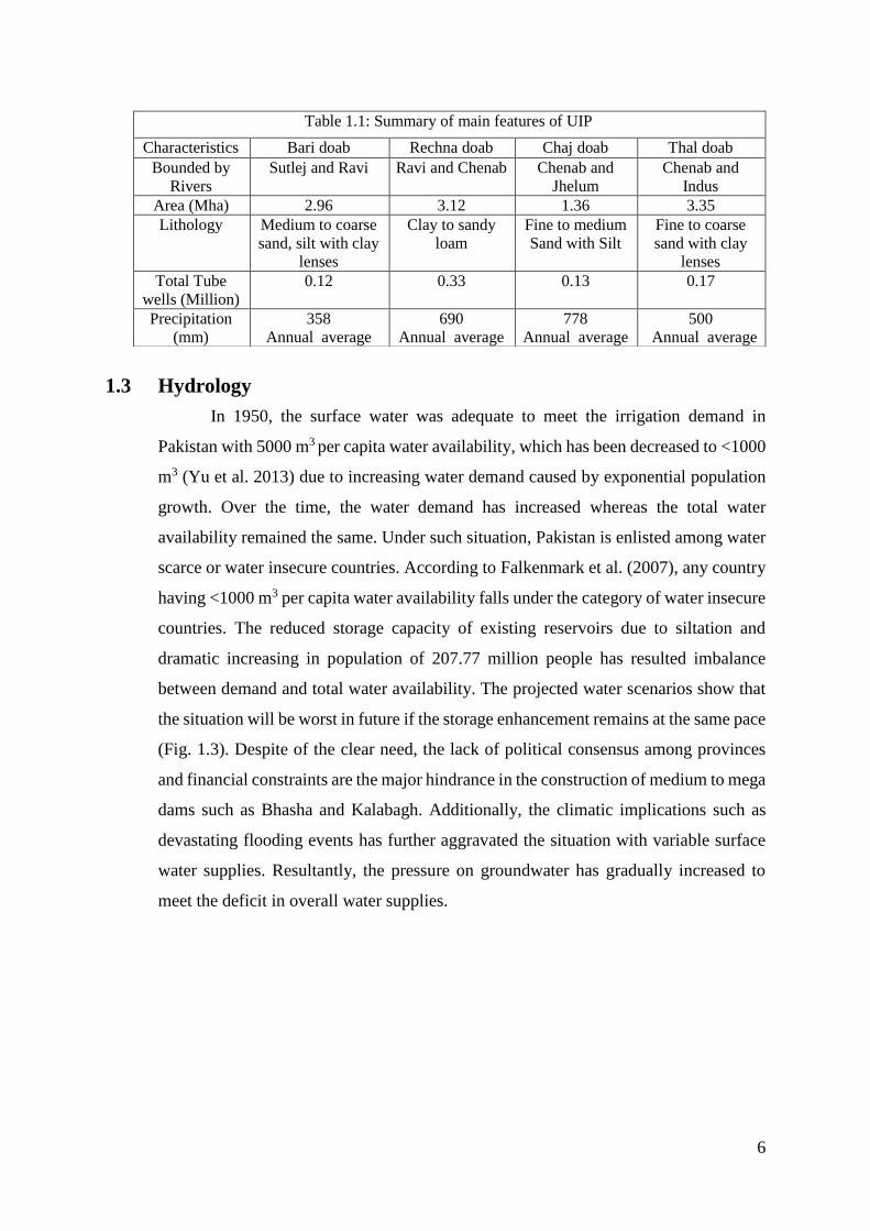
Table 1.1: Summary of main features of UIP
Characteristics Bari doab Rechna doab Chaj doab Thal doab
Bounded by
Rivers
Sutlej and Ravi Ravi and Chenab Chenab and
Jhelum
Chenab and
Indus
Area (Mha) 2.96 3.12 1.36 3.35
Lithology Medium to coarse
sand, silt with clay
lenses
Clay to sandy
loam
Fine to medium
Sand with Silt
Fine to coarse
sand with clay
lenses
Total Tube
wells (Million)
0.12 0.33 0.13 0.17
Precipitation
(mm)
358
Annual average
690
Annual average
778
Annual average
500
Annual average
7
Figure 1.3: Projected scenario of increasing population (red line) versus water availability (blue
color). The population is in million extracted from National Census of 1981, 1998 and 2017
conducted by Population Census Organization (PCO), Pakistan.
The aquifer properties are the important features, which control the groundwater
system response to abstraction and climatic implications (Foster and MacDonald 2014).
The Upper Indus Plain aquifer is an unconfined and well transmissive with generally
fresh quality of groundwater. The alluvial nature and composition of unconsolidated
material has provided favorable sub-surface conditions for storage and water pumping.
The vertical lithological variations in the form of clay lenses somehow limits its scope
at local to regional scale. But the role of this factor is negligible while considering the
huge volume of alluvium in Indus Plain as the average depth to bedrock is 400 meter
(Ahmad 1993). The horizontal permeability is of higher order than vertical. Being
alluvium aquifer, the sandy beds dominate in UIP. However, the existence of clay
lenses in Rechna doab is comparatively higher. In Rechna doab aquifer, the percentage
of sandy beds is about 65-75% (Mundorff et al. 1976). However, the presence of fine
to coarse sandy strata helps to replenish the groundwater system through seepage from
IBIS as well as infiltration from rainfall. The previous studies indicate a general trend
in the hydraulic conductivity of Indus Basin, which varies from >60 to <10 m/day as
we move down from upper to lower Indus basin (Ahmad 1993; Bennett et al. 1967;
Khan et al. 2008). Particularly in UIP, the values of hydraulic conductivity and specific
yield are very high due to alluvial formation (Bonsor et al. 2017). The specific yield
0
500
1000
1500
2000
2500
0
50
100
150
200
250
300
350
400
450
500
1981 1991 1998 2001 2011 2017 2020 2025 2030 2040 2050
Wat
er A
vai
lab
ilit
y (
m3/P
erso
n)
Po
pula
tio
n (
Mil
lio
n)
8
varies over UIP due to the lateral and vertical lithological heterogeneity. The analysis
of 103 pumping tests data conducted by USGS in UIP suggest that the specific yield
ranges from 0.01 to 0.42 with average value of 0.14 (Bennett et al. 1967). The minimum
value of 0.01 pertains to clay deposits whereas 0.42 represents coarse sand.
The presence of extensive irrigation system in the form of IBIS provides a good
source of surface water and groundwater interactions in UIP. In addition to rainfall, a
significant recharge is received through seepage from irrigation system consisting of 5
rivers, 13 barrages and headworks along with 12 link canals in UIP. The role of link
canals is to regulate the surface water supply in the eastern rivers, which are otherwise
having low flows. The link canals appear like rivers as these carry much high surface
water flow than the eastern rivers. After IWT, the flows in eastern rivers are very low
as India has managed to utilize maximum water pertaining to these rivers. Therefore,
the significant flows are only available during the flooding period when India releases
additional water to Pakistan. Consequently, Pakistan faces a massive additional
flooding in Jhelum and Chenab Rivers other than eastern rivers. Due to non-availability
of storages on Chenab, Ravi and Sutlej Rivers, this massive flooding turns into
devastating disaster causing a huge damage to agriculture, livestock, property and
humans. Pakistan receives about 60% of its total annual rainfall only during summer
monsoon period (Latif and Syed 2016). On the other hand, these flooding events are
natural source of aquifer replenishment as well as overhauling of the groundwater
system. Pakistan is among those countries, which are consistently facing flooding
events. Due to global warming, the increasing river flows have augmented the flood
vulnerability. The major recent flooding events include, 1992, 1994, 1995 and 2010
where the floods1992 and 2010 majorly affected the most of the Country (Federal Flood
Commission 2017). The pounding of flood water in the adjacent areas along the rivers
helps to recharge the groundwater system. Figure 1.4 provides the detailed picture of
IBIS.
9
Figure 1.4: Indus Basin Irrigation System (IBIS) in UIP. The irrigation system (river and canals) are
in blue color whereas, the red dots are the locations of barrages.
The climatic implications have further aggravated the situation by not only
shifting the rainfall patterns, seasonal change (Hanif et al. 2013) but its intensity and
duration. The rainfall events are now more intensified with short duration. The summers
have been prolonged where the winters are contracted. Interestingly, the time series
analysis of rainfall (PMD) shows that the amount of annual average rainfall has been
increased from 1971-2015 (Fig. 1.5). Quantitatively, more rainfall is now available but
practically, it is not available at the time when critically required. Hence, the surface
water supplies are irregular and insufficient to meet the existing water demand of
207.77 million people of Pakistan. The data of 19 PMD stations falling in Punjab
province has been used to generate the rainfall time series mentioned below as Fig. 1.5.
The names of these stations include; Lahore, Okara, Multan, Sahiwal, Jhang,
Gujranwala, Faisalabad, Toba Tek Singh, Sargodha, Jhelum, Sialkot, Gujrat, Chakwal,
Mangla, D.G. Khan, Bakhar, Bahawalpur, Bahawalnagar, and Rahimyarkhan.
10
Figure 1.5: Annual average rainfall variations from 1971-2015 in Punjab Province. The blue lines is
the rainfall time series generated using PMD station data. The dotted line in red color shows the
overall rainfall trend.
In Pakistan, the flood irrigation method is commonly used for irrigation. The
share of irrigation water (surface water) is allocated to farmers according to their land
holdings (Bandaragoda 1995). The farmers get their allocated share of irrigation water
once in a week (warabandi system). The increasing food and fiber requirements have
put the farmers naturally under pressure to increase the productivity. Under such
circumstances, the farmers are struggling hard by utilizing all the resources and
exercising all the available options. They are managing fertilizers and applying costly
pesticides/herbicides to increase per acre productivity. The farmers are supplementing
their irrigation demand through abstraction of groundwater (Alam and Olsthoorn 2014).
The ease of availability and flexibility for desired pumping of unregulated
groundwater resource has encouraged accelerated groundwater development in UIP.
Eventually, the cropping intensities have doubled since 1970s (Basharat and Tariq
2015) primarily through extensive groundwater abstraction. This over abstraction of
groundwater has helped significantly in achieving the food security in the Country but
has resulted a number of challenges related to both groundwater quantity and quality
(Khan et al. 2016b). Over time, the exponential growth of private tube-wells dominates
the total number of tube wells, which has reached over one million in UIP from 1985-
2015 (Fig. 1.6). This shows that the dependence on groundwater has significantly
increased over time. Figure 1.7 shows the district-wise distribution of the percentage of
total tube wells available for irrigation supplies (Bureau of Statistics 2012). The Sialkot
is top district with highest (8% of total) number of tube wells followed by Gujranwala
(7%) and Layyah (7%). The districts of Mandi Bahauddin, Muzaffargarh are at third
350
400
450
500
550
600
650
700
750
800
850
900
950
Annual
Aver
age
Rai
nfa
ll (
mm
)
11
(6%) however, 5% of the total number of tube wells exist in each of Sargodha, Jhang,
Narowal and Bakkar districts.
Figure 1.6: Groundwater development in UIP over last three decades (1985-2015)
0.0
0.2
0.4
0.6
0.8
1.0
1.2
198
4-1
985
198
5-1
986
198
6-1
987
198
7-1
988
198
8-1
989
198
9-1
990
199
0-1
991
199
1-1
992
199
2-1
993
199
3-1
994
199
4-1
995
199
5-1
996
199
6-1
997
199
7-1
998
199
8-1
999
199
9-2
000
200
0-2
001
200
1-2
002
200
2-2
003
200
3-2
004
200
4-2
005
200
5-2
006
200
6-2
007
200
7-2
008
200
8-2
009
200
9-2
010
201
0-2
011
201
1-2
012
201
2-2
013
201
3-2
014
201
4-2
015
201
5-2
016N
um
ber
of
To
tal
Tu
bew
ells
(M
illi
on
)
Sialkot8% Gujranwala
7%
Layyah7%
Muzaffargarh6%
Mandi Bahauddin6%
Sargodha5%
Jhang5%
Narowal5%
Bakkar5%
Okara4%
Faisalabad4%
Sheikhupura4%
Kasur3%
Hafizabad3%
Gujrat3%
Khanewal2%
Nankana Sahib2%
D.G. khan2%
Vehari2%
Toba Tek Singh2%
Pakpattan2%
Sahiwal2%
Chiniot2%
Multan2%
Mianwali1%
Lodhran1%
Khushab1%
Lahore1%
Figure 1.7: District-wise Distribution of percentage of total number of tube wells in UIP (2012). The different
colors represent different districts of Punjab province. The percentages show the contribution of number of tube-
wells installed in that particular district.
12
The highest tube well density of 0.10 (tube wells per hectare) is found in Rechna
(Fig. 1.8) where about 33,000 tube wells are pumping groundwater with a total area of
3.12 million hectare. The Rechna doab is a part of famous rice belt (Narowal, Sialkot,
Gujranwala districts, etc.) in Punjab where extensive irrigation is applied for rice crop
using flood irrigation method with almost 90% dependency on groundwater. The Chaj,
Thal and Bari doabs have tube well density of about 0.09, 0.05 and 0.04 tube wells per
hectare respectively.
Figure 1.8: Doab-wise, tube wells density in UIP (2012).
In Pakistan, the contribution of groundwater in total water supplies for irrigation
has reached over 60%. The consistently huge groundwater abstraction has encountered
a number of groundwater management challenges such as groundwater depletion (Khan
et al. 2008; Rodell et al. 2009; Sufi et al. 1998; Tiwari et al. 2009) increased salinity at
shallow depths (Qureshi et al. 2008; Qureshi et al. 2010; Saeed and Ashraf 2005) and
groundwater quality deterioration (Qureshi et al. 2010). The limited surface water
Bari
Rechna
Chaj
Thal
0.00
0.02
0.04
0.06
0.08
0.10
0.12
Upper Indus Plain (Doabs)
Tu
bew
ell
Den
sity
(M
illi
on
Tu
bew
ells
per
Mh
a)
13
supplies against exceeding water demand has become groundwater a main source of
irrigation supplies in the countries like Pakistan (Siebert et al. 2010; Wada et al. 2012).
The imbalance between abstraction and recharge caused by over-exploitation has led
groundwater depletion (Döll et al. 2012; Gleeson et al. 2012; Konikow 2011; Rodell et
al. 2009; Taylor et al. 2013; Wada et al. 2010). The groundwater depletion further
impacts in lowering of groundwater levels (Famiglietti et al. 2011; Scanlon et al. 2010).
With 80 km3 per year abstraction, Pakistan is the fifth largest user of groundwater
globally (Wada et al. 2014). As an immediate impact, the water table is lowering
significantly and the areas under shallow depth to water are decreasing rapidly. The
analysis of depth to water table data collected from International Waterlogging and
Salinity Research Institute a department of Pakistan water and Power Development
Authority (WAPDA), Lahore show that the area coverage under shallow depths (<600
cm or 6 m) has decreased from 1991-2011. A reduction of about 22% in area covered
under shallow depth to water table has been experienced due to groundwater mining
during last two decades in Punjab Province (Fig. 1.9). This change has impacted to
increase the area under deep water table (> 6 m), which is reached up to 52 % of the
total area of Punjab during last two decades (1991-2011).
Figure 1.9: Variations in area coverage under different depth to water table in UIP. The green, purple
and cyan colors show area coverage (%) under maximum depth > 600 cm, 450-600 and 300-450 cm.
It is reported by Qureshi et al. (2010) that in some regions of Punjab, the water
table depletion is prevalent even about 2-3 meters per year, which is an alarming
0%
10%
20%
30%
40%
50%
60%
70%
80%
90%
100%
1991 1992 1993 1994 1995 1996 1997 1998 1999 2000 2006 2007 2008 2009 2010 2011
A
r
e
a
%
0-90 cm 90-150 cm 150-300 cm 300-450 cm 450-600 cm >600 cm
14
situation for groundwater sustainability perspective. Out of 43 canal commands, the
water table depletion in 26 canal commands is reported by Bhutta and Sufi (2004) due
to extensive groundwater abstraction. Khan et al. (2008) has predicted a groundwater
mining situation in lower Rechna doab with water table depletion ranging from 10-20
m over the period 2002 to 2025. A similar situation of significant water table depletion
in central Chaj and lower Bari doabs is reported also due to over exploitation of
groundwater for irrigation supplies (Ashraf and Ahmad 2008; Basharat and Tariq 2013;
Basharat et al. 2014). In Punjab province, about 20% irrigated area is under
groundwater depletion where DTW is more than 12 m (Basharat et al. 2014).
Due to intensive irrigation and excessive groundwater pumping, the average
DTW ranges from 0.5-22.8 meter over UIP as recorded by Punjab Irrigation
Department (PID), Lahore in 2010. The average DTW is about 11.7 meter. The analysis
of spatial variations in DTW show that some regions of UIP aquifer are under stress
where abstraction exceeds the recharge. To analyze the extent of depletion, a
classification has been developed by International Waterlogging and Salinity Research
Institute (IWASRI)-Pakistan by considering the depth to water table, annual depletion
rate and energy requirements for groundwater pumping. According to IWASRI
classification, the areas where DTW >18 meter are considered as highly depleted.
Therefore, it is analyzed that the most of the area of UIP is normal (3-9 m depth)
whereas, some areas of Rechna and Bari doabs are under groundwater depletion (13-
18 m depth) as shown in Fig. 1.10. The lower parts of Bari doab are especially
experiencing the groundwater mining conditions where the groundwater sustainability
is under risk.
15
Figure 1.10: Average depth to water table variations over UIP in 2010. The red color shows highest
depth to water table and is the highly depleted area. The black lines show the different districts of Punjab (Khan et al. 2016a)
In the adjoining areas of River Jhelum, specifically in upper parts of Thal and
Sargodha districts in Chaj doab, the waterlogging also exists because of excessive river
recharge. Similarly, the waterlogging is also reported in the lower parts of Thal doab
(Muzaffargarh district) due to recharge from River Indus. Basically, this is a very small
strip where the distance from the bounding rivers (Indus and Chenab) is very small.
The groundwater recharge is spatially variable in Indus Basin depending upon
the availability of enough rainfall, soil conditions and proximity to surface water or
irrigation system (Basharat and Tariq 2015). The most of the areas of UIP get recharged
through seepage from surface water system by constitutes the recharge from rivers and
canals including return flow from agricultural fields. The rainfall induced recharge is
also available but limited to either upper central parts of doabs due to subsurface
lithological irregularity (existence of clay lenses). In Indus Basin, the surface water
beautifully interacts with groundwater for its replenishment.
The groundwater quality (salinity) also varies in Punjab Province both laterally
and vertically to its marine origin. The Upper Indus Plain was once the part of Arabian
Sea, which gradually retreated and UIP came in to existence. The native groundwater
16
of UIP is saline (Ashraf et al. 2012). However, a thin layer of fresh groundwater has
developed over the time due to the recharge from surface water and rainfall. The
thickness of this fresh groundwater layer varies spatially due to variability in recharge.
In center of the doabs, the layer of fresh quality groundwater is shallow in the center of
doabs whereas it is deeper along the rivers and canals. Generally, the central parts of
all doabs get recharge mainly through rainfall, which is less as compared to recharge
induced by rivers or canals.
1.4 Literature Review
The synthesis of available literature suggest that the most of work done in the
past related to groundwater resource management in Indus Basin, remained mainly
focused on water logging and salinity issue (Qureshi et al. 2008; Qureshi et al. 2010;
Saeed and Ashraf 2005; Sufi et al. 1998), conjunctive use of surface water and
groundwater (Basharat and Tariq 2015; Khan et al. 2008), groundwater modeling by
developing different scenarios (Awan and Ismaeel 2014; Chandio et al. 2012; Khan et
al. 2008). Ashraf and Ahmad (2008) has applied FeFlow groundwater model in
combination with Geographic Information Science (GIS) and Remote Sensing (RS)
techniques to study groundwater variations in Upper Chaj doab. The RS and GIS
derived data inputs such as digital elevation mode (DEM), landuse/landcover and soil
properties were used in the model. They developed different scenarios to analyze the
aquifer response under climatic implications in terms of extreme events
(floods/droughts). The variable patterns of groundwater abstractions were also studied
and groundwater budget was computed in Upper Chaj doab. Basharat and Tariq (2015)
studied fluctuations and analyzed the variations in irrigation pumping cost at head,
middle and tail end farmers of lower Bari doab canal (LBDC). The crop water deficit
approach was used to estimate the groundwater pumping in the study area. This study
concluded that the tail-end farmers bear 2.19 times higher cost for irrigation as
compared to head-end farmers. They highlight that the groundwater depletion is more
critical at tail-end due to less availability of surface water supplies. Resultantly, the
farmers will have to bear additional cost. As an outcome, appropriate management
strategies were proposed based on the development of future scenarios.
Similarly in Rechna doab, a comprehensive study was performed (Khan et al.
2008) by using a dynamic approach to study the groundwater dynamics in Rechna doab.
In the context of excessive groundwater pumping at escalating rate, this study was
17
conducted to assess the future groundwater trends. The major findings of this study
include; depletion of groundwater levels from 10-20 m due to the limited availability
of surface water supplies in the Lower Rechna doab whereas, the Upper Rechna doab
is projected under high risk to salinization due to salt-water upconing. This upward
movement of salinization is caused by overexploitation of groundwater. The study
further concluded that if the current trends of groundwater pumping persistently prevail
in future, the leakage from river would help decrease the groundwater salinity in the
lower and middle parts of Rechna doabs. Another study was conducted by Awan and
Ismaeel (2014) in Rechna doab with focus on the assessment of groundwater recharge
in Lower Chenab Canal (LCC). The study demonstrated a new technique to map
groundwater recharge through Soil and Water Assessment Tool (SWAT) model in
combination with Surface Energy Balance Algorithm (SEBAL). They estimated
groundwater recharge through SWAT model at high spatial scale whereas a comparison
of SWAT simulated evapotranspiration with SEBAL was also performed, which
resulted a good agreement. The study concluded that an increase of about 40% in
groundwater recharge is projected in the study area. These studies have provided a very
good insight details and contributed effectively for understating the complexities of
issues and appropriate management options. However, these studies are limited in their
spatial scope and remained only focused to case study scale by covering hardly a canal
command area or a portion of doab. Recently, efforts have been made for Indus basin
scale groundwater accounting and quantification of spatial abstraction (Cheema et al.
2014). To quantify the spatial abstraction in Indus Basin, Cheema et al. (2014) used
methodology consisting of remotely sensed evapotranspiration and precipitation
products, hydrological modeling and spatially derived information pertaining to canal
water supply. They applied SWAT model as a major tool for hydrological modeling
and simulated basin scale important hydrological components. This study demonstrated
the technique to quantify the spatial patterns of groundwater abstract at high spatial
resolution of 1 km. This study concluded that during a period of one-year 2007, the
groundwater of about 68 km3 was abstracted along with groundwater depletion of about
31 km3 in the whole Indus Basin. Furthermore, the areas of Pakistani and Indian Punjab
and Haryana (India) were declared as most vulnerable to groundwater depletion.
Khan et al. (2016a) conducted a comprehensive study of groundwater resource
assessment by applying an integrated methodology consisting of geophysical surveys
18
for the quantification of usable groundwater for irrigation and drinking requirements,
application of isotope hydrology for the identification of groundwater recharge
mechanism and groundwater modeling for doab scale water balance estimation. The
study reported that the lower parts of Bari and Chaj, some parts of Rechna and Upper
Thal doabs are under groundwater stress where the high groundwater depletion was
noted in Bari doab. Khan et al. (2016b) developed a first physical based groundwater
modeling of whole Punjab Province.
These studies have successfully accounted the basin-wide groundwater
budgeting at annual scale but their reliability has hampered due to input data scarcity
(Khan et al. 2016b). The physical groundwater modeling requires a lot of observational
input data sets on various parameters for model development as well as its calibration
and validation purpose, which is hardly available in developing countries like Pakistan
(Brunner et al. 2007; Moore and Fisher 2012). The availability of spatially well
distributed and reliable input information is primarily important for groundwater
modeling to produce reliable strategies (Singh 2014; Wondzell et al. 2009). The
reliability of input data is directly proportional to the accuracy of modeling results.
Traditionally, the hydrological observations are available in the form of point
measurements however; the models require more distributed type regional information
or picture for accurate simulation. Usually, the models accept point data and then it is
interpolated to generate spatially distributed information. The physical groundwater
modeling is very effective for the assessment, monitoring and devising management
strategies but input data scarcity limits its role for basin scale applications.
Despite of the selection of a very good groundwater model with high
professional expertise, the lack of sufficient and reliable input information could
hamper the credibility by producing under/over estimations of modeling results (Singh
2014). In developing countries like Pakistan, the data paucity is a big challenge for the
hydrologists. The ground observations are limited in their spatial and temporal domains
due to week measurement network related most of the critically required parameters
such as rainfall, temperature, groundwater levels, stream discharges, etc. In Pakistan,
Scarp Monitoring Organization (SMO), a department of Pakistan Water and Power
Development Authority (WAPDA), Lahore has maintained a network of piezometers
in the Indus Basin. They have installed these piezometers with the objective to cover
all canal command areas. SMO collect depth to water table (DTW) information along
19
with groundwater quality biannually. These piezometers were installed a long time ago
during 1980s. Most of them are now redundant due to lack of proper maintenance.
Those, which are still operational, the data is only available before and after monsoon
period. The role of summer monsoon in the groundwater hydrology of Indus Basin is
very imperative. It comes with heavy rainfalls and lasts for almost three months from
July to September. It facilitates to somehow in the replenishment of groundwater
system as a significant rise in water levels is observed. Such a data at biannual
frequency is practically insufficient to support any management strategy.
Another issue with piezometric point information is its sensitivity to local
events/phenomena. The point data is always good to capture the local events therefore,
the water level fluctuation method is not considered very accurate for regional
assessment of groundwater depletion. This is due to very reason that the regional
phenomenon dominates the local, which reduces the accuracy of results at regional
scale. Therefore, the hydrologist more relay on groundwater models for accurate
quantification of recharge or groundwater abstract and future predictions.
The geophysical and isotopic applications are also very good in performance
for the groundwater resource assessment and analyzing the recharge mechanism. The
environmental isotopes are very help to determine the groundwater flow patterns and
studying the long-term groundwater system behavior. The methods are field oriented
as the field surveys are their integral part. The field activities involve a lot of time,
human resource and financial requirements, which limits their role as a continuous
activity for basin scale groundwater monitoring and management.
The lack of centralized water resource information system is another challenge
for the hydrologist while analyzing the long-term system behavior and its dynamics
under climatic variabilities. Due to non-appreciable trend of data sharing, a lot of efforts
are required to gather required information form relevant agencies in Pakistan. The non-
availability of data in digital format (mostly in hardcopy) is another challenge.
Recently, Pakistan Council of Research in Water Resources (PCRWR), a national
research organization working under Ministry of Science and Technology, Government
of Pakistan has taken an initiative in collaboration with Asian Development Bank
(ADB) to develop a common water resource data platform. The objective of this effort
is to provide a centralize water resource information system to facilitate the researchers,
hydrologists and policy makers for long-term planning and management activities. As
20
per plans, it is initially started from Balochistan and further will be expanded to national
scale by bringing all the provinces together.
The remote sensing technology has become very popular among researchers and
is increasingly used in hydrological applications. The literature suggest that the remote
sensing based products have been used as input datasets for groundwater modeling in
Indus Basin (Ashraf and Ahmad 2008; Awan and Ismaeel 2014; Cheema et al. 2014)
and in Ganges Basin (Bhanja et al. 2017; Bhanja et al. 2016a; Bhanja et al. 2016b;
Mukherjee et al. 2015). In integration with groundwater modeling, remote sensing is
also used for the improvement (such as calibration and validation) of groundwater
models (Brunner et al. 2007). However, the researchers have not yet benefited fully
from the true potential of remote sensing technology.
The Gravity Recovery and Climate Experiment (GRACE) is the National
Aeronautics and Space Administration (NASA) twin gravity satellite, which was
launched in 2002 in collaboration with German Space Centre (GFZ). It very accurately
maintains its distance between two satellites through laser. The GRACE is very
sensitive to changes in gravity and if a small change in gravity happens on or below the
surface, it gets recorded as anomaly (Rodell et al. 2009). Very uniquely, it senses the
complete water cycle by all covering its all components. The GRACE is very effective
tool to get the information about complete vertical profile starting from snow/glaciers
down up to groundwater (Longuevergne et al. 2010). The GRACE is capable to provide
gravity anomalies, which are useful to extract changes in Total Water Storage (TWS)
at 10 daily to monthly scale. The GRACE has facilitated the research by bridging the
input data gaps and very useful for global hydrological applications due to its global
coverage (Famiglietti et al. 2011; Rodell et al. 2009; Tiwari et al. 2009). By design, the
GRACE is a coarse spatial resolution satellite (~300-350 km). It is said that the changes
in gravity are induced by the redistribution of mass under, on and above the earth
surface (Wahr et al. 1998). The basic principal of the GRACE based groundwater
monitoring is assumed that the changes in gravity are essentially induced by changes in
mass of subsurface rocks, which is dependent on water content. A water bearing rock
have higher density (mass) then dry rock and therefore, changes in density cause
variations in gravity to which the GRACE is sensitive enough.
The GRACE data collection mechanism is also unique. GRACE mission is a
combination of two satellite, which are about 220 km apart from each another with
21
altitude of about 450 km. The distance between two satellites is maintained through a
very precise laser system. When there is any change (more mass) in gravity due to
variations in mass over or under the earth surface, the leading satellite slows down
however, the following satellite continue its speed until it approaches the same region
of leading satellite. Due to this change in distance induced by change in gravity, it is
recorded as gravity anomaly. Similarly, when the leading satellite crosses the high mass
region, it again follows its normal speed by creating a variation in the distance with
following satellite. As the following satellite is still in the high mass and high density
region, so its speed is bit slower the leading satellite. Therefore, in a similar fashion,
GRACE collects the gravity data (anomalies) due to changes in distance induced by
variations in mass on the earth surface. The temporal frequency of GRACE data is 10
daily to monthly however, the data becomes publically available after 1-2 months as lot
of initial data processing is involved.
Having global coverage with reasonable spatio-temporal frequency, the
GRACE is potentially appropriate to apply for basin scale water accounting. It is widely
used as a credible tool for the quantification of groundwater abstraction and recharge
processes globally. Recently, many studies have demonstrated its potential as a
scientific tool for successful monitoring of groundwater resource, its abstraction,
groundwater dynamics, spatio-temporal changes in different components of water
cycle, drought monitoring and assessment of flooding impacts in relation to
groundwater recharge (Famiglietti et al. 2011; Feng et al. 2013; Rodell et al. 2009;
Scanlon et al. 2012; Strassberg et al. 2009; Strassberg et al. 2007; Tiwari et al. 2009).
The GRACE has been extensively used for groundwater depletion in various regions of
the world and famous river basins such as Indus Basin (Jin and Feng 2013; Rodell et
al. 2009; Tiwari et al. 2009), High Plain Aquifer (Strassberg et al. 2009; Strassberg et
al. 2007), Central Valley-California (Famiglietti et al. 2011; Scanlon et al. 2012),
Mississippi River Basin (Rodell et al. 2007), Illinois State (Swenson et al. 2006), Congo
Basin (Lee et al. 2011), North China (Feng et al. 2013), etc.
The situation analysis identifies the gaps to apply the GRACE satellite as a
scientific and cost-effective tool for groundwater resource management in Indus Basin
of Pakistan where the in-situ data and groundwater modeling tools are limited to large
spatial domains.
22
1.5 Problem Statement
The groundwater aquifers provide a cushion during extreme climatic events and
ensure the agricultural sustainability by regulating the irrigation supplies in agrarian
countries like Pakistan. Therefore, the agricultural sustainability is directly linked with
the sustainability of groundwater relating to food security perspective. For sustainable
groundwater resource management, the groundwater abstraction and recharge are the
primarily important parameters of groundwater budgeting. However, the non-
availability of reliable and frequent information in spatio-temporal domains, poses a
big challenge for basin wide accounting and devising appropriate management
strategies in developing countries like Pakistan. The input data paucity, limitations of
groundwater models, complexities of the groundwater system itself and climatic
implications, provides motivation to explore alternate tools. The situation analysis
identifies the gap to apply Gravity Recovery and Climate Experiment (GRACE)
satellite as a scientific and cost-effective tool for groundwater resource management in
Indus Basin of Pakistan where the in-situ data and groundwater modeling tools are
limited to cover large spatial domains. This study evaluates the potential of GARCE
satellite-based methodology as science grade tool for the monthly monitoring of
groundwater storage changes as well as its effectiveness at operational groundwater
management scales like doabs.
1.6 Objectives
The specific objectives of this study are;
a) To evaluate the GRACE satellite integrated VIC model approach for the
estimation of groundwater storage (GWS) at regional to sub-regional scales.
b) To assess the impact of the GRACE based GW storage estimation and
monitoring methodology to enable decision making over conventional
approaches.
c) To design statistical approach for the prediction of 30-180 days groundwater
storage variations and estimate its level of uncertainty to enable decision-
making.
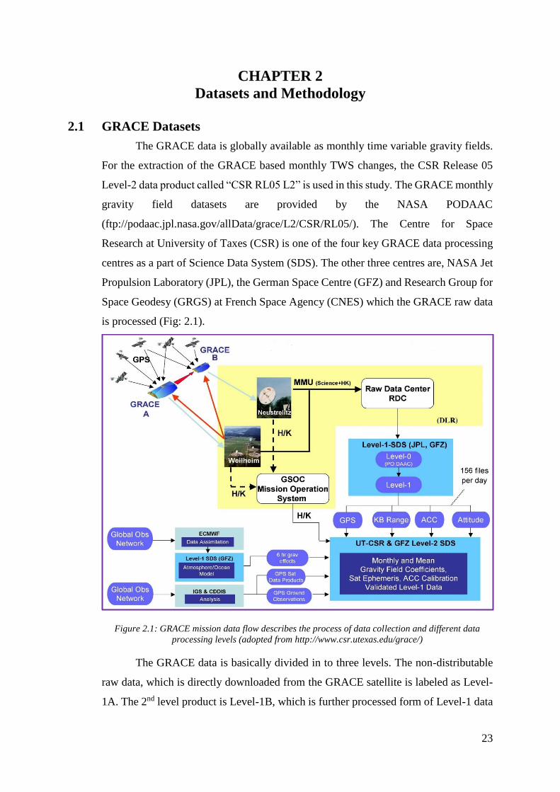
23
CHAPTER 2
Datasets and Methodology
2.1 GRACE Datasets
The GRACE data is globally available as monthly time variable gravity fields.
For the extraction of the GRACE based monthly TWS changes, the CSR Release 05
Level-2 data product called “CSR RL05 L2” is used in this study. The GRACE monthly
gravity field datasets are provided by the NASA PODAAC
(ftp://podaac.jpl.nasa.gov/allData/grace/L2/CSR/RL05/). The Centre for Space
Research at University of Taxes (CSR) is one of the four key GRACE data processing
centres as a part of Science Data System (SDS). The other three centres are, NASA Jet
Propulsion Laboratory (JPL), the German Space Centre (GFZ) and Research Group for
Space Geodesy (GRGS) at French Space Agency (CNES) which the GRACE raw data
is processed (Fig: 2.1).
Figure 2.1: GRACE mission data flow describes the process of data collection and different data
processing levels (adopted from http://www.csr.utexas.edu/grace/)
The GRACE data is basically divided in to three levels. The non-distributable
raw data, which is directly downloaded from the GRACE satellite is labeled as Level-
1A. The 2nd level product is Level-1B, which is further processed form of Level-1 data
24
to produce monthly gravity field estimates in form of spherical harmonic coefficients.
The 2nd level data is actually produced by combining the mean or static gravity
estimates based on several years. Under CSR RL05 Level-2 data products, there are
three types of monthly datasets available such as GSM, GAC and GAD. The GSM
contains the coefficients for the earth monthly gravity field with the highest coefficients
of degree and order 96. The GAC is just the average monthly solution of gravity fields
whereas, the GAD is an ancillary data product that represents the mean ocean bottom
pressure. The GRACE data (CSR-RL05 Level-2) in the form of monthly gravity fields
or anomalies from 2003-2010 is used in this study.
2.2 Piezometric Datasets
The piezometric water level data is used for the calibration and validation of the
GRACE derived groundwater storages information. This data is collected from SCARP
Monitoring Organization (SMO), Pakistan Water and Power Development Authority
(WAPDA). On the basis of long-term data availability and spatially well distributed,
about 167 piezometric locations have been selected and used covering the whole Upper
Indus Plain (Punjab Province). The water level measurements in the form of depth to
water table (DTW) are collected and available only on bi-annual frequency, which is
pre-monsoon (May-July) and post-monsoon (September-December). The SMO has
installed these piezometers strategically by covering all the canal command areas in
Punjab. There are two main reasons for this biannual data collection. Firstly, the data
collection form these piezometers is manual. Therefore, the data collection at 10-daily
to monthly scale will require lot of resources, which are not easy to manage. Secondly,
the groundwater system is mainly influenced by monsoon system. A considerable
change in the water levels appears while comparing pre-monsoon and post-monsoon
season. Another challenge is that even at biannual scale, the DTW data collection takes
2-3 months to cover whole UIP. Under such situation, those months have been selected
for comparison with the GRACE data during which most of the records were available.
2.3 Variable Infiltration Capacity (VIC) Model Datasets
In this study, the role soil moisture (SM) and surface runoff (SR) information is
very important. This information is required to separate groundwater signal from the
GRACE derived TWS. This information is derived through hydrological modeling by
25
applying the VIC model. The VIC model was developed by Liang et al. (1994). The
VIC simulated monthly SM and SR data from 2003-2010 is used in this study.
2.4 Methodology
The methodology of this study includes mainly two components. The first
component explains the data processing related GRACE gravity fields and then
extraction of TWS anomalies. However, the second component deals with the
hydrological modeling for the simulation of soil moisture information and surface water
fluxes. The detailed flow chart methodology is given at Fig. 2.2.
Under this satellite integrated numerically down-scaling techniques, it is
explained here that GRACE-TWS solution (1°×1° or 300 km × 300 km) has been first
retrieved from its original gravity anomalies by using CSR-RL05 data having 3°×3°
spatial resolution at monthly scale. This has been achieved by involving several
processing steps, filtering techniques and signal restoration. However, the third level of
GRACE-based GWS at 0.1°×0.1° (10 km × 10 km) has been derived by using numerical
down-scaling technique in which the VIC model simulated output of soil moisture and
surface fluxes (0.1°×0.1°) has been used. Finally, GRACE derived GWS anomalies
have been estimated to analyze the temporal changes in groundwater storage underlying
of Upper Indus Plain in Pakistan. This technique is called dynamic numerical
downscaling in with simulation of physical parameters through dynamic hydrological
has been integrated with satellite data to effectively estimate the changes in terms of
groundwater storage anomalies.
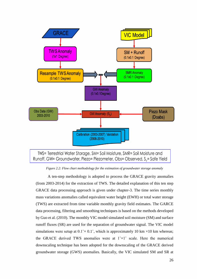
26
Figure 2.2: Flow chart methodology for the estimation of groundwater storage anomaly
A ten-step methodology is adopted to process the GRACE gravity anomalies
(from 2003-2014) for the extraction of TWS. The detailed explanation of this ten step
GRACE data processing approach is given under chapter-3. The time series monthly
mass variations anomalies called equivalent water height (EWH) or total water storage
(TWS) are extracted from time variable monthly gravity field estimates. The GARCE
data processing, filtering and smoothing techniques is based on the methods developed
by Guo et al. (2010). The monthly VIC model simulated soil moisture (SM) and surface
runoff fluxes (SR) are used for the separation of groundwater signal. The VIC model
simulations were setup at 0.1˚× 0.1˚, which is approximately 10 km ×10 km whereas;
the GRACE derived TWS anomalies were at 1˚×1˚ scale. Here the numerical
downscaling technique has been adopted for the downscaling of the GRACE derived
groundwater storage (GWS) anomalies. Basically, the VIC simulated SM and SR at
27
0.1˚× 0.1˚ scale has been used as guiding information for the downscaling of the
GRACE TWS available at 1˚×1˚ scale. For this purpose, the GRACE TWS (1˚×1˚) cell
were resampled to the resolution of the VIC to maintain the consistency. It is mentioned
here that before the separation of GWS, SM and SR have been added to make SMR and
then subtracted from long-term average to estimate SMR anomalies. This was helpful
to make the datasets comparable with the GRACE TWS anomalies.
According to Rodell et al. (2009) and Longuevergne et al. (2010), the changes
in TWS is a function of changes in Soil Moisture (SM), Surface Water (SW),
Groundwater Storage (GWS), Snow water Equivalent (SWE) and Biosphere (BIO).
ΔTWS =ΔGWS+ΔSM+ΔSW+ΔSWE+ΔBIO (2.1)
Based on the hydrological characteristics of the study area, it is assumed that
the soil moisture, surface runoff and groundwater abstraction are the dominant
components controlling the hydrology of Upper Indus Plain. Therefore, the equation
2.1 becomes;
ΔGWS =ΔTWS - (ΔSM+ΔSW) (2.2)
Finally, by following equation (2.2), the groundwater storage anomalies have
been extracted. For calibration and validation purpose, the DTW data is used from
2003-2010. Due to the lack of temporal uniformity in piezometric recordings, the
seasonal average method is used for both DTW and the GRACE-GWS. To compare the
GRACE derived groundwater storage anomalies with piezometric data, the depth to
water table information was converted in to water level and then estimated storage
change using average specific yield. The further details pertaining to the calculation of
the GRACE as well as piezomtric groundwater storage anomalies are available as
Appendix-E. According to Bennett et al. (1967), the value of average specific yield is
calculated as 0.14 for UIP which ranges from 0.01 to 0.42. As such, there is no
systematic spatial variability analyzed in the study area. However, the specific yield
varies with lithological changes especially decreases with clay content which is not
having any regular trend. The clay exists in the form of irregular clay lenses having
vertical and lateral heterogeneity (Bennett et al. 1967). Therefore, there is considerable
vertical hydrogeological heterogeneity in the UIP due to the presence of clay lenses.
28
Due to these uncertainties, the average value of safe yield as 0.12 has been used for
calculations on the safe side.
After the conversion of piezometric DTW into groundwater storage anomalies,
the calibration with the GRACE-GWS was performed from 2003-2010 at each doab
scale. Based on the calibration results, a statistical relationship (Figs. 5.27, 5.29, 5.31
& 5.33) has been developed, which is validated over the period 2008-2010 to make
groundwater projection for next 6 months. This is might be helpful for the groundwater
managers to devise appropriate strategies by knowing about the expected changes in
the groundwater system. This technique has been tested at each doab scale (Figs. 5.19,
5.20, 5.23 & 5.24) and its accuracy depends upon the accuracy of the GRACE-GWS.
By following this methodology, two different scenarios have been tested (Table
5.1). Under first scenario, the performance of the GRACE-GWS is evaluated with is-
situ water level observations at actual the GRACE resolution (1˚×1˚ scale) at the scale
of UIP. Whereas in second scenario, the GRACE-GWS anomalies are estimated at
0.1˚× 0.1˚ and then accuracy evaluation has been performed at each doab scale to see
the feasibility of the GRACE-GWS for operational groundwater resource management
in Indus Basin. These doabs are the effective operational scales in Pakistan referring to
sustainable groundwater management in Upper Indus Plain aquifer. For automatic data
processing and raster analysis, the model builder and spatial analyst extensions of Arc
GIS software (version 10.4) have been used. The “asci files” pertaining to TWS
anomaly and the VIC simulations have been converted in to raster format for further
spatial analysis. By using model builder utility, various models have been developed in
Arc GIS for automatic data processing, analysis and extraction of SMR, TWS and GWS
anomalies over UIP as well as doab scales over study area (Appendix-A).
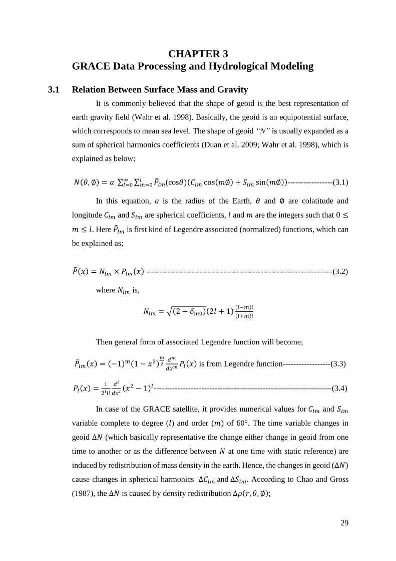
29
CHAPTER 3
GRACE Data Processing and Hydrological Modeling
3.1 Relation Between Surface Mass and Gravity
It is commonly believed that the shape of geoid is the best representation of
earth gravity field (Wahr et al. 1998). Basically, the geoid is an equipotential surface,
which corresponds to mean sea level. The shape of geoid “N” is usually expanded as a
sum of spherical harmonics coefficients (Duan et al. 2009; Wahr et al. 1998), which is
explained as below;
𝑁(𝜃, ∅) = 𝑎 ∑ ∑ �̃�𝑙𝑚𝑙𝑚=0
∞𝑙=0 (cos𝜃)(𝐶𝑙𝑚 cos(𝑚∅) + 𝑆𝑙𝑚 sin(𝑚∅)) -----------------(3.1)
In this equation, a is the radius of the Earth, 𝜃 and ∅ are colatitude and
longitude 𝐶𝑙𝑚 and 𝑆𝑙𝑚 are spherical coefficients, 𝑙 and 𝑚 are the integers such that 0 ≤
𝑚 ≤ 𝑙. Here �̃�𝑙𝑚 is first kind of Legendre associated (normalized) functions, which can
be explained as;
�̃�(𝑥) = 𝑁𝑙𝑚 × 𝑃𝑙𝑚(𝑥) ----------------------------------------------------------------------(3.2)
where 𝑁𝑙𝑚 is,
𝑁𝑙𝑚 = √(2 − 𝛿𝑚0)(2𝑙 + 1)(𝑙−𝑚)!
(𝑙+𝑚)!
Then general form of associated Legendre function will become;
�̃�𝑙𝑚(𝑥) = (−1)𝑚(1 − 𝑥2)𝑚
2𝑑𝑚
𝑑𝑥𝑚 𝑃𝑙(𝑥) is from Legendre function------------------(3.3)
𝑃𝑙(𝑥) =1
2𝑙𝑙!
𝑑𝑙
𝑑𝑥𝑙(𝑥2 − 1)𝑙-------------------------------------------------------------------(3.4)
In case of the GRACE satellite, it provides numerical values for 𝐶𝑙𝑚 and 𝑆𝑙𝑚
variable complete to degree (𝑙) and order (𝑚) of 60°. The time variable changes in
geoid ∆𝑁 (which basically representative the change either change in geoid from one
time to another or as the difference between 𝑁 at one time with static reference) are
induced by redistribution of mass density in the earth. Hence, the changes in geoid (∆𝑁)
cause changes in spherical harmonics ∆𝐶𝑙𝑚 and ∆𝑆𝑙𝑚. According to Chao and Gross
(1987), the ∆𝑁 is caused by density redistribution ∆𝜌(𝑟, 𝜃, ∅);
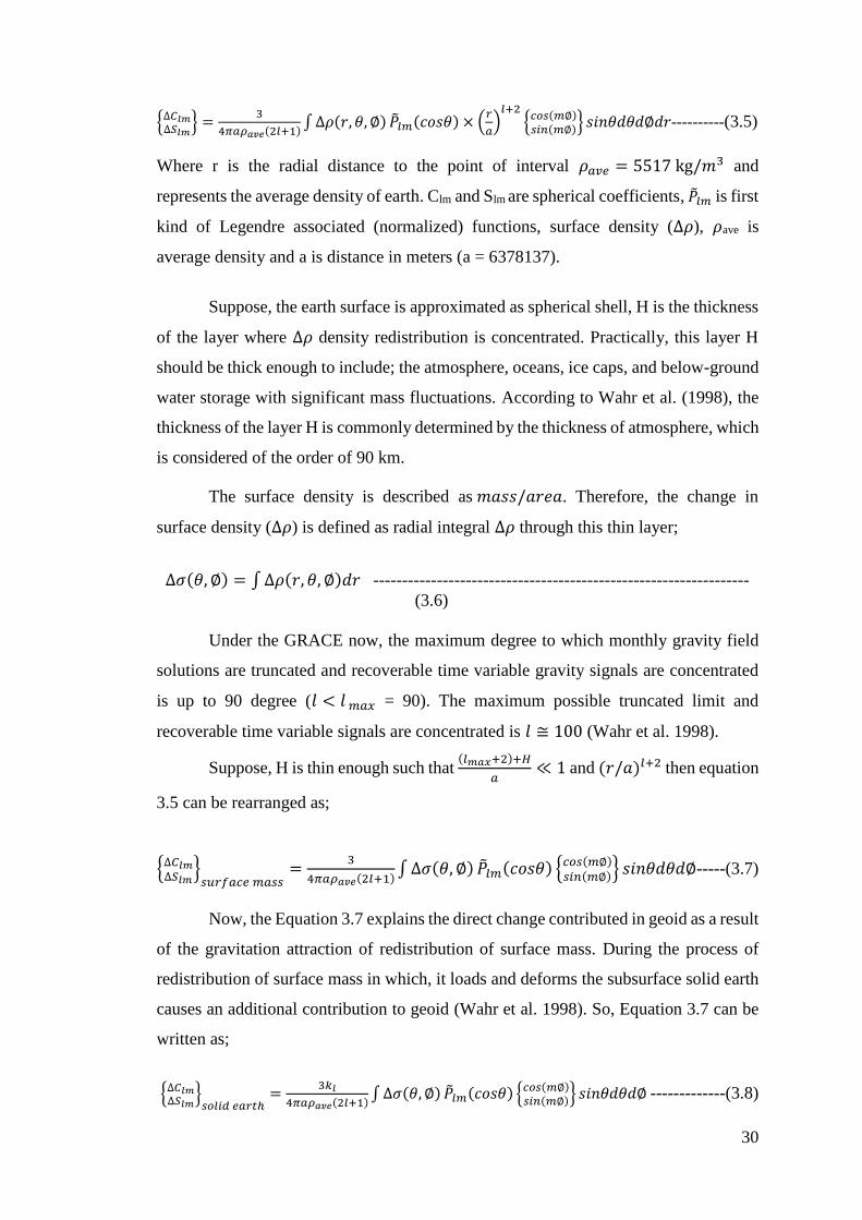
30
{∆𝐶𝑙𝑚∆𝑆𝑙𝑚
} =3
4𝜋𝑎𝜌𝑎𝑣𝑒(2𝑙+1)∫ ∆𝜌(𝑟, 𝜃, ∅) �̃�𝑙𝑚(𝑐𝑜𝑠𝜃) × (
𝑟
𝑎)
𝑙+2{𝑐𝑜𝑠(𝑚∅)
𝑠𝑖𝑛(𝑚∅)} 𝑠𝑖𝑛𝜃𝑑𝜃𝑑∅𝑑𝑟----------(3.5)
Where r is the radial distance to the point of interval 𝜌𝑎𝑣𝑒 = 5517 kg/𝑚3 and
represents the average density of earth. Clm and Slm are spherical coefficients, �̃�𝑙𝑚 is first
kind of Legendre associated (normalized) functions, surface density (∆𝜌), 𝜌ave is
average density and a is distance in meters (a = 6378137).
Suppose, the earth surface is approximated as spherical shell, H is the thickness
of the layer where ∆𝜌 density redistribution is concentrated. Practically, this layer H
should be thick enough to include; the atmosphere, oceans, ice caps, and below-ground
water storage with significant mass fluctuations. According to Wahr et al. (1998), the
thickness of the layer H is commonly determined by the thickness of atmosphere, which
is considered of the order of 90 km.
The surface density is described as 𝑚𝑎𝑠𝑠/𝑎𝑟𝑒𝑎. Therefore, the change in
surface density (∆𝜌) is defined as radial integral ∆𝜌 through this thin layer;
∆𝜎(𝜃, ∅) = ∫ ∆𝜌(𝑟, 𝜃, ∅)𝑑𝑟 -----------------------------------------------------------------
(3.6)
Under the GRACE now, the maximum degree to which monthly gravity field
solutions are truncated and recoverable time variable gravity signals are concentrated
is up to 90 degree (𝑙 < 𝑙 𝑚𝑎𝑥 = 90). The maximum possible truncated limit and
recoverable time variable signals are concentrated is 𝑙 ≅ 100 (Wahr et al. 1998).
Suppose, H is thin enough such that (𝑙𝑚𝑎𝑥+2)+𝐻
𝑎≪ 1 and (𝑟/𝑎)𝑙+2 then equation
3.5 can be rearranged as;
{∆𝐶𝑙𝑚∆𝑆𝑙𝑚
}𝑠𝑢𝑟𝑓𝑎𝑐𝑒 𝑚𝑎𝑠𝑠
=3
4𝜋𝑎𝜌𝑎𝑣𝑒(2𝑙+1)∫ ∆𝜎(𝜃, ∅) �̃�𝑙𝑚(𝑐𝑜𝑠𝜃) {𝑐𝑜𝑠(𝑚∅)
𝑠𝑖𝑛(𝑚∅)} 𝑠𝑖𝑛𝜃𝑑𝜃𝑑∅-----(3.7)
Now, the Equation 3.7 explains the direct change contributed in geoid as a result
of the gravitation attraction of redistribution of surface mass. During the process of
redistribution of surface mass in which, it loads and deforms the subsurface solid earth
causes an additional contribution to geoid (Wahr et al. 1998). So, Equation 3.7 can be
written as;
{∆𝐶𝑙𝑚∆𝑆𝑙𝑚
}𝑠𝑜𝑙𝑖𝑑 𝑒𝑎𝑟𝑡ℎ
=3𝑘𝑙
4𝜋𝑎𝜌𝑎𝑣𝑒(2𝑙+1)∫ ∆𝜎(𝜃, ∅) �̃�𝑙𝑚(𝑐𝑜𝑠𝜃) {𝑐𝑜𝑠(𝑚∅)
𝑠𝑖𝑛(𝑚∅)} 𝑠𝑖𝑛𝜃𝑑𝜃𝑑∅ -------------(3.8)
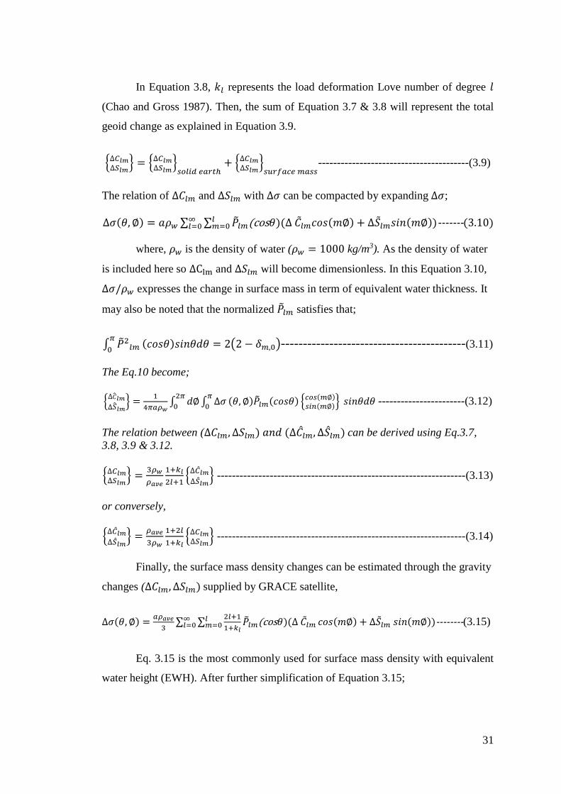
31
In Equation 3.8, 𝑘𝑙 represents the load deformation Love number of degree 𝑙
(Chao and Gross 1987). Then, the sum of Equation 3.7 & 3.8 will represent the total
geoid change as explained in Equation 3.9.
{∆𝐶𝑙𝑚∆𝑆𝑙𝑚
} = {∆𝐶𝑙𝑚∆𝑆𝑙𝑚
}𝑠𝑜𝑙𝑖𝑑 𝑒𝑎𝑟𝑡ℎ
+ {∆𝐶𝑙𝑚∆𝑆𝑙𝑚
}𝑠𝑢𝑟𝑓𝑎𝑐𝑒 𝑚𝑎𝑠𝑠
----------------------------------------(3.9)
The relation of ∆𝐶𝑙𝑚 and ∆𝑆𝑙𝑚 with ∆𝜎 can be compacted by expanding ∆𝜎;
∆𝜎(𝜃, ∅) = 𝑎𝜌𝑤 ∑ ∑ �̃�𝑙𝑚𝑙𝑚=0
∞𝑙=0 (cos𝜃)(∆ �̃�𝑙𝑚𝑐𝑜𝑠(𝑚∅) + ∆�̃�𝑙𝑚𝑠𝑖𝑛(𝑚∅))-------(3.10)
where, 𝜌𝑤 is the density of water (𝜌𝑤 = 1000 kg/m3). As the density of water
is included here so ∆Clm and ∆𝑆𝑙𝑚 will become dimensionless. In this Equation 3.10,
∆𝜎/𝜌𝑤 expresses the change in surface mass in term of equivalent water thickness. It
may also be noted that the normalized �̃�𝑙𝑚 satisfies that;
∫ �̃�2𝑙𝑚
𝜋
0(𝑐𝑜𝑠𝜃)𝑠𝑖𝑛𝜃𝑑𝜃 = 2(2 − 𝛿𝑚,0)------------------------------------------(3.11)
The Eq.10 become;
{∆�̂�𝑙𝑚
∆�̂�𝑙𝑚} =
1
4𝜋𝑎𝜌𝑤∫ 𝑑∅ ∫ ∆𝜎
𝜋
0
2𝜋
0(𝜃, ∅)�̃�𝑙𝑚(𝑐𝑜𝑠𝜃) {𝑐𝑜𝑠(𝑚∅)
𝑠𝑖𝑛(𝑚∅)} 𝑠𝑖𝑛𝜃𝑑𝜃 -----------------------(3.12)
The relation between (∆𝐶𝑙𝑚, ∆𝑆𝑙𝑚) 𝑎𝑛𝑑 (∆�̂�𝑙𝑚, ∆�̂�𝑙𝑚) can be derived using Eq.3.7,
3.8, 3.9 & 3.12.
{∆𝐶𝑙𝑚∆𝑆𝑙𝑚
} =3𝜌𝑤
𝜌𝑎𝑣𝑒
1+𝑘𝑙
2𝑙+1{
∆�̂�𝑙𝑚
∆�̂�𝑙𝑚} ------------------------------------------------------------------(3.13)
or conversely,
{∆�̂�𝑙𝑚
∆�̂�𝑙𝑚} =
𝜌𝑎𝑣𝑒
3𝜌𝑤
1+2𝑙
1+𝑘𝑙{∆𝐶𝑙𝑚
∆𝑆𝑙𝑚} ------------------------------------------------------------------(3.14)
Finally, the surface mass density changes can be estimated through the gravity
changes (∆𝐶𝑙𝑚, ∆𝑆𝑙𝑚) supplied by GRACE satellite,
∆𝜎(𝜃, ∅) =𝑎𝜌𝑎𝑣𝑒
3∑ ∑
2𝑙+1
1+𝑘𝑙
𝑙𝑚=0
∞𝑙=0 �̃�𝑙𝑚(cos𝜃)(∆ �̃�𝑙𝑚 𝑐𝑜𝑠(𝑚∅) + ∆�̃�𝑙𝑚 𝑠𝑖𝑛(𝑚∅))--------(3.15)
Eq. 3.15 is the most commonly used for surface mass density with equivalent
water height (EWH). After further simplification of Equation 3.15;
32
∆ℎ(𝜃, ∅) =𝑎𝜌𝑎𝑣𝑒
3𝜌𝑤∑ ∑
2𝑙+1
1+𝑘𝑙
𝑙𝑚=0
∞𝑙=0 �̃�𝑙𝑚(cos𝜃)(∆ �̃�𝑙𝑚𝑐𝑜𝑠(𝑚∅) + ∆�̃�𝑙𝑚𝑠𝑖𝑛(𝑚∅)) --------(3.16)
This is final expression used for the defining the relation between surface mass
density, gravity and water height.
3.2 Processing of Spherical Harmonic Coefficients
The codes developed by Duan et al. (2009) are used for the GRACE data
processing. The details of step by step data processing approach are shown in Fig. 3.1.
Figure 3.1: Step by step methodological approach for the GRACE data processing
3.2.1 Step-0: Rename Data Files
This step is merely to change the name and extension of data file to make them
end with _0.txt. The GRACE L2 monthly GSM-2 data files include the following date
span information;
GSM-2_2002095-2002121_0021_UTCSR_0096_0005
where,
GSM-2 = Data product level 2 containing highest monthly
gravity fields
2002095 = Starting date (95th day of 2002)
2002121 = End date (121st day of 2002)
33
0021 = Number of days with data: 21
UTCSR = University of Taxes, CSR data product
0096 = Maximum degree and order of SHCs
0005 = Number of release
The average of the starting and end dates is used as the date of the solution for
each month (for above example, 107 will be considered as solution date for this file).
The output files have the following format YYYY DDD XXX.txt, where YYYY is the
year, DDD is the median date of data span, and XXX is a user assigned suffix. The
input information is given in the file Rename L2 Files.txt. The first line (cp) is the
command for copying files of the OS. For example, windows: copy, Unix/Linux: cp.
The second line has two integers. The first one is the location of the first digit of year
in the original data file name and the second one is the number of digits of year. The
third line has two integers. The first one is the location of the first digit of the first day
in the original data file name. The second one is the number of digits for the first day.
The fourth line has two integers. The first one is the location of the first digit of the last
day in the original data file name. The second one is the number of digits for the last
day. Whereas, the fifth and sixth lines are string to be included as suffix in output file
names, i.e., XXX and number of data files. The following lines are the data files. One
file name per line. An example of the content of Rename L2 Files.txt is as under;
copy
6 4
10 3
18 3
_0
83
GSM-2_2002102-2002120_0018_UTCSR_0096_0005
GSM-2_2002121-2002139_0019_UTCSR_0096_0005
Rename L2 Files.cpp is the program name used for completing Step-0.
3.2.2 Step-1: Extract SHCs
This step is to process the data file for the extraction of Spherical Harmonics
Coefficients (SHCs) using the code Extract SHCs.cpp. Input and output file names are
assigned in the file Extract_SHCs.txt. The first line is the maximum degree and order.
34
The second line is the total number of data files, and the following are input and output
names for each data file. The following is an example of Extract_SHCs.txt file:
60
83
2002_289_0.txt 2002_289_1.txt
2002_319_0.txt 2002_319_1.txt
The output format is l m c s in each line. Data in output files are in the order m
= 0, 1, 2, and then l = m, m+1, ....
The output of this step is stored in the files as suffix _1.txt.
3.2.3 Step-2 & 3: Geocentre & Truncation
The step-2 is performed to replace degree 1 and 2 terms with Satellite Laser
Ranging (SLR) estimates. The 3rd step is to truncate the SHCs up to degree 60 by
eliminating the degrees from 61 to 96. The reason is that the higher degree and order
coefficients include larger error, which are preferred to be omitted in certain
applications. So, there is a need to truncate the SHCs to a lower maximum degree and
order. For Step-2 &3, Geocentre_J2_CSR.cpp and Truncate SHCs.cpp; codes are used
for data processing. The output file contains the following information;
The first line is the maximum degree of input SHCs. The second line is the
maximum degree of output SHCs. The third line is the number of files of SHCs. The
rest of the lines are the data lines.
3.2.4 Step-4 & 5: Average Calculation and Reference Subtraction
Under Step-4; the GRACE L2 data are normally used for studying mass
changes. So, a reference field is normally subtracted from all the monthly solutions. In
most cases, the reference field is the average in a certain time span and the same long-
term monthly average is calculated. The mean SHCs are calculated from all 140
monthly files from all 140 monthly SHCs. The Step-5 is performed to get the monthly
anomalies of SHCs by subtracting the average (Step-4) from all 140 monthly files. In
this way, Step-4&5 are to get monthly anomalies. The codes, Average_SHCs.cpp and
Subtract_Reference_SHCs.cpp are used to get output files. The output file after Step-5
is named as 2003_107_4.txt.
35
3.2.5 Step-6 & 7: Remove PGR and Decorrelation Filter
Step-6 is performed to remove Post Glacial Rebound (PGR) from signal using
PGR model or Glacial Isostatic Adjustment (GIA) called Paulson_60 (which is only
generated up to 60 degrees). PGR data is available in terms of crustal uplift and relative
sea level (RSL) rise. For PGR, sea surface is assumed equipotential and is referred to
as geoid. The PGR-geoid follows global sea level rise, it differs from the geodetic geoid
by an offset. Actually, in PGR models, RSL changes are equivalent to PGR-geoid
changes with respect to the crust, which are provided even on continent as well. The
geoid change is referred as the sum of crustal uplift and RSL changes.
The purpose of decorrelation filter is to remove the correlated errors in the data.
Based on Duan et al. (2009) the designed filter is very much capable to left portions of
lower degree and order unchanged whereas as the remaining are filtered using a moving
window with polynomial fit high pass filtering technique (Shum et al. 2011). The data
filtering by decorrelation is essentially required to remove the correlated errors
associated with spherical harmonic coefficients (SHCs) of higher degree and order.
These higher degree and order SHCs are affected more by correlated noises than lower
degree and order (Kummerow et al. 1998; Shum et al. 2011; Swenson et al. 2006;
Wouters et al. 2014). These correlated errors are further studied by Duan et al. (2009)
and revealed that the SHCs with same degree and parity are also correlated with each
other. The output fine was resulted as 2003_107_6.txt after Step-7.
3.2.6 Step-8 & 9: Transform SHCs to Mass and Mass to Grids
The Step-8 is to computer Equivalent Water Height (EWH) or Terrestrial
Storage (TWS) anomalies (mm). The data is then converted from SHCs to monthly
mass changes (anomalies). The Step-9 is to transform the mass anomalies in to regular
1˚ × 1˚ grids. It helps to map the GRACE TWS monthly anomalies for further analysis
the temporal changes in terrestrial water storage over any specific region of interest.
The output file of Step-9 is named as 2003_107_8.txt.
For error analysis, the review of literature reveals that GRACE time series
contains both errors of random as well as systematic nature. The random errors are
associated with spectral degree (Wahr et al. 2006) whereas, the systematic errors
increase as a function of spectral order (Swenson and Wahr, 2006). Under such a
scenario, post-processing techniques including (Gaussian Smoothing, De-Correlation
36
and Leakage Reduction) are applied to original GRACE spherical harmonic
coefficients to improve the signal to noise ratio.
3.2.7 Step-10: Gaussian Smoothing and Leakage Reduction
The data smoothing is basically post-processing technique, which is applied
after the extraction of equivalent water height (EWH) or total water storage (TWS)
anomalies. This technique is primarily applied on the GRACE data for accuracy
improvement by reducing the signal noises of various types (Duan et al. 2009; Kusche
2007; Shum et al. 2011). The GRACE L2 data has some North-South stripes, which
could potentially introduce errors at lower latitudes (East-West direction) resulting low
resolution as compared to South-North direction with high resolution. According to
Shum et al. (2011), if a non-isotropic spatial smoothing filter is applied to the processed
data at longitudinal direction than in latitudinal, it could potentially produce better
results by keeping more signal information. As the SHCs are limited to degree and order
60 during the truncation process, it means that the spatial resolution of the field is 3° ×
3° or 330 km by 330 km. Therefore, a non-isotropic filter with radius 300 km is applied
to smoothen the data and leakage reduction (Duan et al. 2009; Guo et al. 2010). The
final output file is produced with name 2003_107_9.txt. After completing all above
mentioned ten step methodology, the output text (.txt) were then converted in to shape
files (.shp) for further data clipping to focus study region (UIP, Pakistan) using Arc GIS
10.3 software. By applying interpolation technique in Arc GIS software, the monthly
raster files were generated to study the changes in TWS over UIP from 2002-2014.
The de-correlation technique based on high pass filter is also applied to remove
correlated errors associated with higher order (Duan et al. 2009; Kusche 2007; Shum et
al. 2011).
3.3 Signal Restoration
The signal restoration is also one of the post processing technique to restore the
GRACE TWS signal, which was dumped during the process of data smoothing through
Gaussian filtering. The process used for signal restoration is termed as scaling factor.
As suggested by Long et al. (2014), the scaling factor for Indus Basin has been
estimated as 1.131 (Table 3). This scaling factor is derived based on the output of six
global hydrological models (GHM) models, which includes; Noah 2.7, VIC, Mosaic,
CLM 2.0, CLM 4.0, and WGHM2.2 (Long et al. 2014). After the calculation of scaling
37
factor, simple arithmetic operation has been applied to achieve the signal restoration by
multiplying the TWS with scaling factor (1.131). Basically, the scaling factor helps to
restore the amplitude of the GRACE signal, which was dumped at the stage of data
smoothing. The signal restoration is essentially required step to ensure the accuracy of
output signal.
3.4 Variable Infiltration Capacity Model (VIC)
The Variable Infiltration Capacity (VIC, version 4.0.6) model has been used to
simulate soil moisture and surface water fluxes to derive groundwater storage from the
GRACE-TWS. The VIC is a macroscale semi distributed hydrological model
developed by (Liang et al. 1994). In previous studies, the VIC has been extensively
used for hydrological forecasting, budgeting of water and energy and assessment of
climate change impacts in many regions of the world such as Ganges, Brahmaputra and
Meghna Basins (Siddique-E-Akbor et al. 2014), China (Wang et al. 2012; Zhang et al.
2014; Zhao et al. 2013) and Red River Basin (Xue et al. 2016). The VIC is sensitive
enough to incorporate sub-grid variability, control soil water storage as well as runoff
generation. As a basic feature of the VIC model, it models land surface as lumped by
considering uniform and flat cells of greater than 1 km (Siddique-E-Akbor et al. 2014).
The main model climatic data inputs include; topography, rainfall (daily to sub-daily),
snow, temperature and wind speed. As an output, the model simulates water balance at
daily to sub-daily time steps at each grid cell scale. Under a recent application of the
VIC model in Ganges–Brahmaputra–Meghna river basins, the study concluded that the
VIC has successfully captured daily runoff and stream flow dynamics (Siddique-E-
Akbor et al. 2014).
For this study, it is anticipated that there is no interconnection between grids
other than river routing and water can only enter in to a grid cell through atmosphere.
Also, the groundwater flow is considered to be relatively small as compared to surface
and near surface flows. There is no groundwater recharge from channel network.
It is important to mention that the above mentioned assumptions are quite
acceptable for hydrological modeling approaches (Siddique-E-Akbor et al. 2014).
Basically, the VIC is a large-scale (i.e, mesoscale; >>1 km; usually ≥10 km) hydrologic
model which allows to ignore the non-channel flow between the neighboring cells. It
means that, “The portions of surface and subsurface runoff that reach the local channel
network within a grid cell are assumed to be very large in comparison with the portions
38
that cross grid cell boundaries into neighboring cells”. Therefore, we can assume that;
there is no interconnection between grids other than river routing. Secondly, as there is
no inter-connection between the grids, and the streamflow routing is performed
separately using a separate routing model. Therefore, water in the land surface model
(i.e., VIC) can only enter a grid cell through the atmosphere. Thirdly, the assumption
that, “groundwater flow is relatively small compared to surface and near-surface flows”
also holds true during the monsoon period.
Fourthly, since the model grid cells are very large in size (i.e., ≥10 km).
Therefore, we can say that, “the portions of surface and subsurface runoff that reach the
local channel network within a grid cell are assumed to be >> the portions that return
into the cell as groundwater recharge. This assumption was only made for only the
simplification of the VIC model. Fifthly, the assumption regarding soil column depth
also holds valid as the hydrological models did not account for water storage variations
in deep unsaturated soil. However, sub-root-zone soil dries only by gravity drainage or
by diffusion to drier layers above. The lack of a drying trend in the root zone indicates
that deep soil-water storage was likewise stable (Rodell et al. 2009). The VIC setup was
calibrated with respect to the observed flow. As long as the soil moisture anomaly plot
is stable (i.e., no increasing or decreasing trend), the depth is acceptable for calculating
GW fluctuation. Sixthly, the two layers of soil were considered in the VIC model setup
with 30 cm and 70 cm depth reasoning that the model was calibrated against streamflow
and the deep soil-water storage was found stable. In other words, the impact of the depth
or number of layers does not become very much significant for the calculation of GW
storage anomalies.
3.4.1 VIC Model Simulation and Calibration
Under present study, the VIC model was setup specifically for Indus Basin at
0.1 degree resolution (10 km) for daily time steps considering total soil thickness of 1
m. Vertically, the soil profile was divided in to two layers where first layers cover depth
up to 0.3 m and second layer extends up to 0.7 m thickness. As pre-requisite input data
requirements of the VIC model, the topographic information was derived from Shuttle
Radar Topographic Mission (SRTM) of 90 meter resolution whereas, the global land
cover classification (GLCC) map was used to incorporate land cover information of
Indus Basin in the model. The spatial resolution of GLCC data (version-1) is
(https://Ita.cr.urgs.gov/GLCC) 400 m. The global soil data product called harmonized
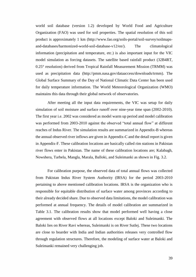
39
world soil database (version 1.2) developed by World Food and Agriculture
Organization (FAO) was used for soil properties. The spatial resolution of this soil
product is approximately 1 km (http://www.fao.org/soils-portal/soil-survey/soilmaps-
and-databases/harmonized-world-soil-database-v12/en/). The climatological
information (precipitation and temperature, etc.) is also important input for the VIC
model simulation as forcing datasets. The satellite based rainfall product (32B4RT,
0.25° resolution) derived from Tropical Rainfall Measurement Mission (TRMM) was
used as precipitation data (http://pmm.nasa.gov/dataaccess/downloads/trmm). The
Global Surface Summary of the Day of National Climatic Data Center has been used
for daily temperature information. The World Meteorological Organization (WMO)
maintains this data through their global network of observatories.
After meeting all the input data requirements, the VIC was setup for daily
simulation of soil moisture and surface runoff over nine-year time span (2002-2010).
The first year i.e. 2002 was considered as model warm up period and model calibration
was performed from 2003-2010 against the observed “total annual flow” at different
reaches of Indus River. The simulation results are summarized in Appendix-B whereas
the annual observed river inflows are given in Appendix-C and the detail report is given
in Appendix-F. These calibration locations are basically called rim stations in Pakistan
river flows enter in Pakistan. The name of these calibration locations are; Kalabagh,
Nowshera, Tarbela, Mangla, Marala, Balloki, and Suleimanki as shown in Fig. 3.2.
For calibration purpose, the observed data of total annual flows was collected
from Pakistan Indus River System Authority (IRSA) for the period 2003-2010
pertaining to above mentioned calibration locations. IRSA is the organization who is
responsible for equitable distribution of surface water among provinces according to
their already decided share. Due to observed data limitations, the model calibration was
performed at annual frequency. The details of model calibration are summarized in
Table 3.1. The calibration results show that model performed well having a close
agreement with observed flows at all locations except Baloki and Suleimanki. The
Baloki lies on River Ravi whereas, Suleimanki is on River Sutlej. These two locations
are close to boarder with India and Indian authorities releases very controlled flow
through regulation structures. Therefore, the modeling of surface water at Baloki and
Suleimanki remained very challenging job.
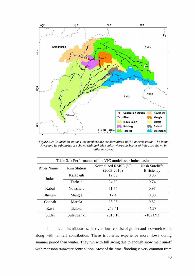
40
Figure 3.2: Calibration stations, the numbers are the normalized RMSE at each station. The Indus
River and its tributaries are shown with dark blue color where sub-basins of Indus are shown in
different colors
In Indus and its tributaries, the river flows consist of glacier and snowmelt water
along with rainfall contribution. These tributaries experience more flows during
summer period than winter. They run with full swing due to enough snow melt runoff
with monsoon rainwater contribution. Most of the time, flooding is very common from
Table 3.1: Performance of the VIC model over Indus basin
River Name Rim Station Normalized RMSE (%)
(2003-2010)
Nash Sutcliffe
Efficiency
Indus Kalabagh 12.66 0.86
Tarbela 24.32 0.74
Kabul Nowshera 51.74 0.97
Jhelum Mangla 17.4 0.98
Chenab Marala 25.98 0.82
Ravi Baloki 248.41 -4.57
Sutlej Suleimanki 2919.19 -1021.92
41
last few years and Pakistan is experiencing frequent flooding events of different
intensities and affecting different parts of the Country. It is also declared 7th most
vulnerable country with respect to climate change. The monsoon triggered flash
flooding not only result in massive economic loss but also impacts humans in terms of
large death toll. The flood of 2003 and 2007 affected Sindh and Khyber Pakhtunkhwa
(KPK) provinces where district of Thatta and some areas of KPK were affected the
most due to flash flooding. Pakistan has experienced a massive and devastating flooding
event in July, 2010 which has affected major part of the Country including KPK, Punjab
and Sindh provinces. From 2010-2014, frequent flooding is experienced more common
at almost every year but with varying intensity. The performance evaluation parameters
such as Nash–Sutcliffe efficiency and Root Mean Square Error (RMSE) were applied.
The Nash-Sutcliffe Efficiency (NSE) is calculated using the formula (Moriasi et al.
2007).
𝑁𝑆𝐸 = 1 − [∑ (𝑄𝑖
𝑜𝑏𝑠 − 𝑄𝑖𝑠𝑖𝑚)
2𝑛𝑖=1
∑ (𝑄𝑖𝑜𝑏𝑠 − �̅�)
2𝑛𝑖=1
]
where
𝑄𝑖𝑜𝑏𝑠
is the observed discharge value at i time step
𝑄𝑖𝑠𝑖𝑚
is the simulated discharge value at i time step
�̅� is the mean of the observed discharge values
The model resulted with Nash–Sutcliffe efficiency of more than 0.74 where
RMSE ranges from 12% to 50%. Keeping in view the fact that there is always room
available for the improvement of hydrological models in snow dominated regions
(Yang et al. 2013; Yu et al. 2013), the results simulated by the VIC model are
considered acceptable for further inclusion and derivation of groundwater storage
anomalies from the GRACE data. In comparison with the GLDAS (which is regional
model with more global focus), the performance of the VIC in simulating soil moisture
and surface dynamics is better because, it is specifically setup for Indus Basin with high
spatial sensitivity of 1˚ × 0.1˚ grid (under Chapter-4, more detailed discussion is
available referring to the comparison of the VIC with GLDAS derived groundwater
storage anomalies).
For analysis consistency with the GRACE, the monthly VIC simulated soil
moisture and surface runoff fluxes at the scale of 0.1 degree have been used for further
analysis and soil moisture and runoff anomalies were calculated as per already
explained methodology. The calculated soil moisture and runoff anomalies (SMR) were
42
further used for the extraction of GWS anomalies. Figure 3.3 is the example of resultant
SMR anomalies for the month of February, 2003 over Indus Basin at the scale of 0.1˚×
0.1˚ whereas Figure. 3.4 explains the variations in average SMR anomalies from 2003-
2010 at the scale of 1˚ × 1˚. The analysis reveals that maximum variations in average
SMR anomalies (2003-2010) is noticed in the Punjab Province (Upper Indus Plain) of
Pakistan and India, which is attributed to significant variations in precipitation,
topography and lithology. Figure 3.5 represents the average variations in SMR anomaly
more specifically over UIP (0.1˚ × 0.1˚ scale). It indicates that the soil moisture and
surface runoff (SMR anomalies) has changed more rapidly as compared to Bari doab
with least in Thal. In comparison with others two, Chaj and Rechna doabs are under
intensive agriculture and were also exposed to flooding during 2010 flood in Pakistan.
This area is also famous for rice crop, which is irrigated through traditional flood
irrigation method and standing water is maintained in the paddies for a couple of
months. In Thal doab, the reason for less change in SMR anomaly is due to Thal desert.
Most of the area under sand dunes is dependent on rain-fed agriculture. Due to low
rainfall and having rain-fed agriculture, there is less change in groundwater storage in
Thal doab. The topography of the UIP is flat with warm climate and the variations in
soil moisture is the dominant factor for variations in SMR anomaly.
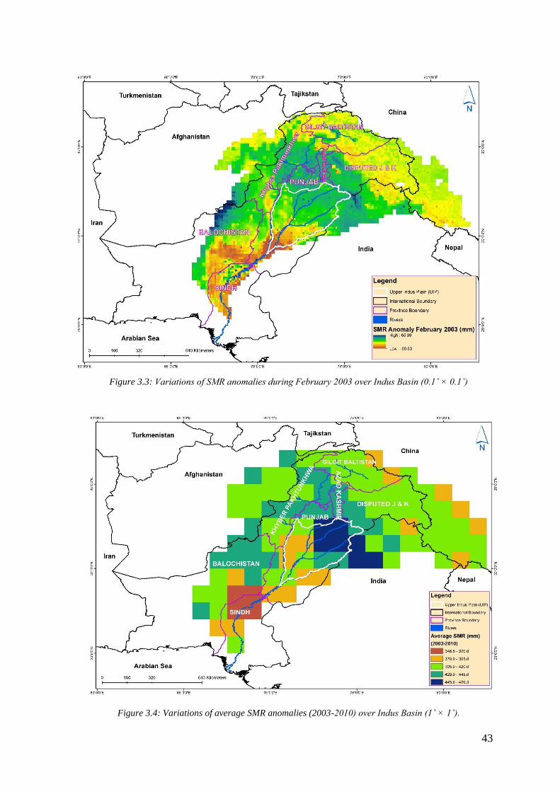
43
Figure 3.3: Variations of SMR anomalies during February 2003 over Indus Basin (0.1˚ × 0.1˚)
Figure 3.4: Variations of average SMR anomalies (2003-2010) over Indus Basin (1˚ × 1˚).
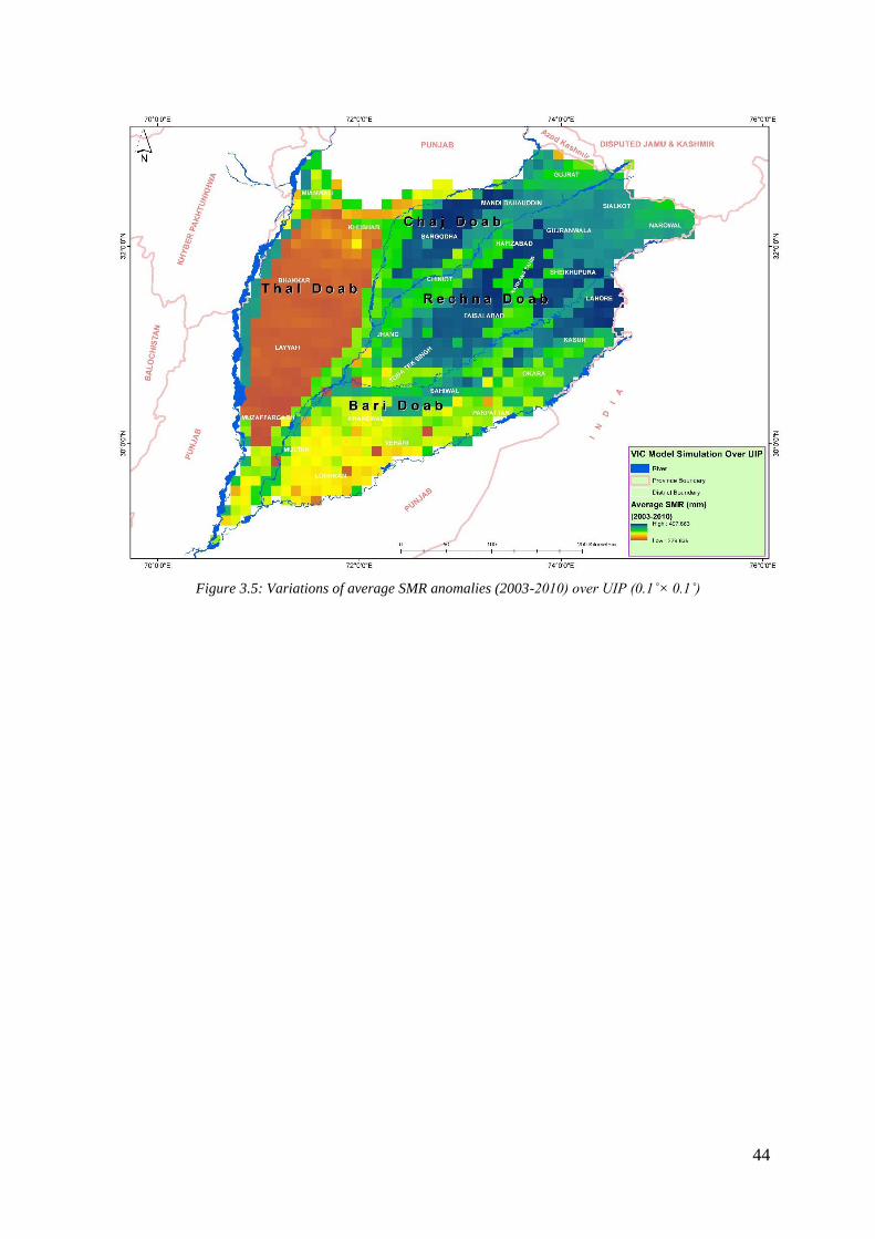
44
Figure 3.5: Variations of average SMR anomalies (2003-2010) over UIP (0.1˚× 0.1˚)
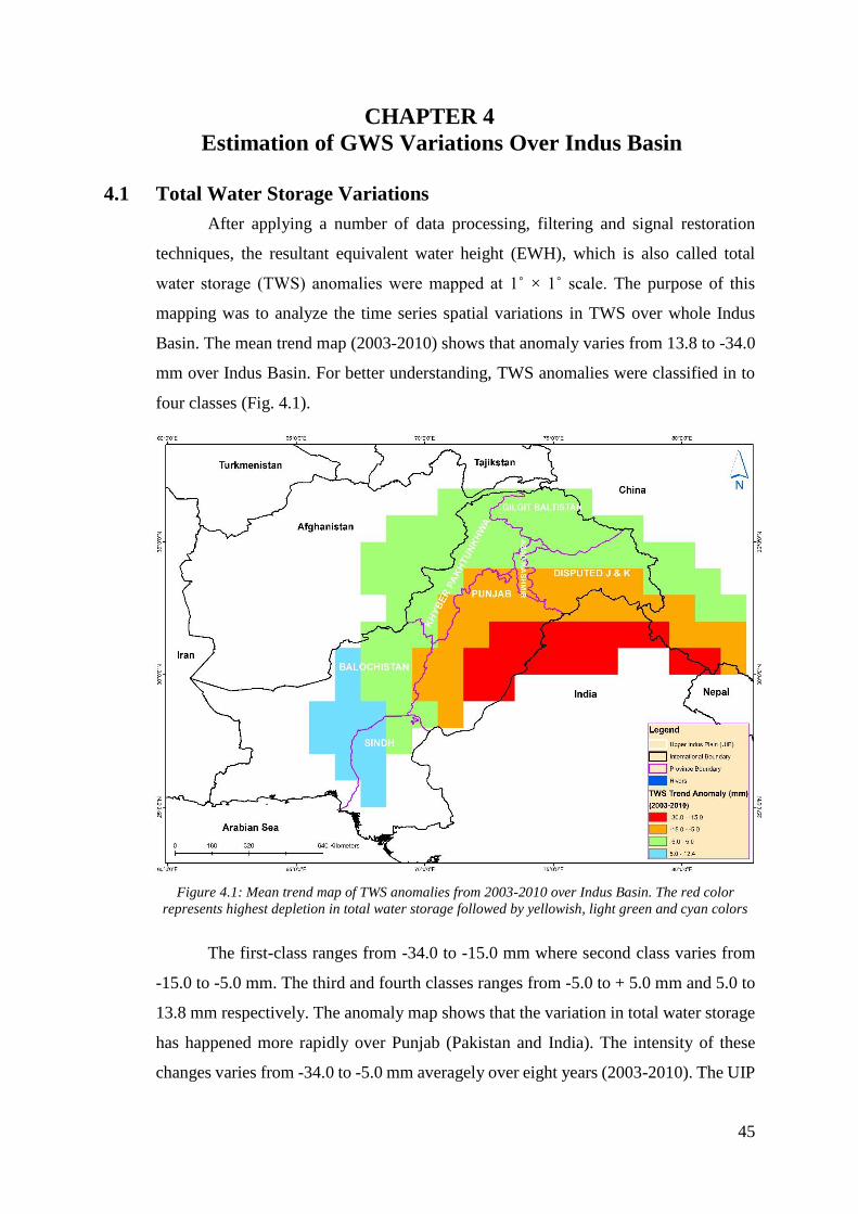
45
CHAPTER 4
Estimation of GWS Variations Over Indus Basin
4.1 Total Water Storage Variations
After applying a number of data processing, filtering and signal restoration
techniques, the resultant equivalent water height (EWH), which is also called total
water storage (TWS) anomalies were mapped at 1˚ × 1˚ scale. The purpose of this
mapping was to analyze the time series spatial variations in TWS over whole Indus
Basin. The mean trend map (2003-2010) shows that anomaly varies from 13.8 to -34.0
mm over Indus Basin. For better understanding, TWS anomalies were classified in to
four classes (Fig. 4.1).
Figure 4.1: Mean trend map of TWS anomalies from 2003-2010 over Indus Basin. The red color
represents highest depletion in total water storage followed by yellowish, light green and cyan colors
The first-class ranges from -34.0 to -15.0 mm where second class varies from
-15.0 to -5.0 mm. The third and fourth classes ranges from -5.0 to + 5.0 mm and 5.0 to
13.8 mm respectively. The anomaly map shows that the variation in total water storage
has happened more rapidly over Punjab (Pakistan and India). The intensity of these
changes varies from -34.0 to -5.0 mm averagely over eight years (2003-2010). The UIP
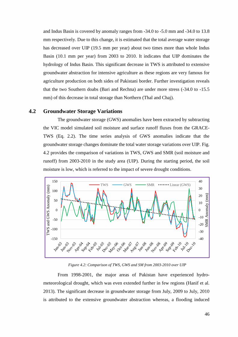
46
and Indus Basin is covered by anomaly ranges from -34.0 to -5.0 mm and -34.0 to 13.8
mm respectively. Due to this change, it is estimated that the total average water storage
has decreased over UIP (19.5 mm per year) about two times more than whole Indus
Basin (10.1 mm per year) from 2003 to 2010. It indicates that UIP dominates the
hydrology of Indus Basin. This significant decrease in TWS is attributed to extensive
groundwater abstraction for intensive agriculture as these regions are very famous for
agriculture production on both sides of Pakistani border. Further investigation reveals
that the two Southern doabs (Bari and Rechna) are under more stress (-34.0 to -15.5
mm) of this decrease in total storage than Northern (Thal and Chaj).
4.2 Groundwater Storage Variations
The groundwater storage (GWS) anomalies have been extracted by subtracting
the VIC model simulated soil moisture and surface runoff fluxes from the GRACE-
TWS (Eq. 2.2). The time series analysis of GWS anomalies indicate that the
groundwater storage changes dominate the total water storage variations over UIP. Fig.
4.2 provides the comparison of variations in TWS, GWS and SMR (soil moisture and
runoff) from 2003-2010 in the study area (UIP). During the starting period, the soil
moisture is low, which is referred to the impact of severe drought conditions.
Figure 4.2: Comparison of TWS, GWS and SM from 2003-2010 over UIP
From 1998-2001, the major areas of Pakistan have experienced hydro-
meteorological drought, which was even extended further in few regions (Hanif et al.
2013). The significant decrease in groundwater storage from July, 2009 to July, 2010
is attributed to the extensive groundwater abstraction whereas, a flooding induced
-40
-30
-20
-10
0
10
20
30
40
-150
-100
-50
0
50
100
150
SM
R A
no
mal
y (
mm
)
TW
S a
nd
GW
S A
no
mal
y (
mm
) TWS GWS SMR Linear (GWS)
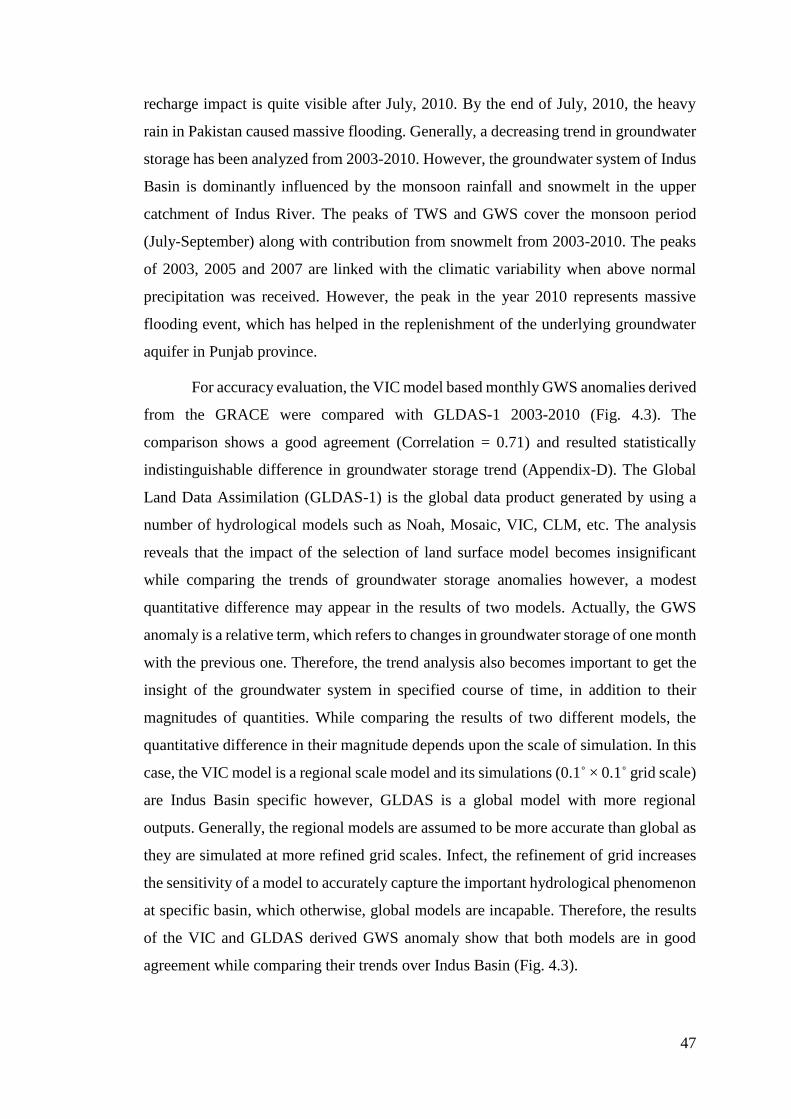
47
recharge impact is quite visible after July, 2010. By the end of July, 2010, the heavy
rain in Pakistan caused massive flooding. Generally, a decreasing trend in groundwater
storage has been analyzed from 2003-2010. However, the groundwater system of Indus
Basin is dominantly influenced by the monsoon rainfall and snowmelt in the upper
catchment of Indus River. The peaks of TWS and GWS cover the monsoon period
(July-September) along with contribution from snowmelt from 2003-2010. The peaks
of 2003, 2005 and 2007 are linked with the climatic variability when above normal
precipitation was received. However, the peak in the year 2010 represents massive
flooding event, which has helped in the replenishment of the underlying groundwater
aquifer in Punjab province.
For accuracy evaluation, the VIC model based monthly GWS anomalies derived
from the GRACE were compared with GLDAS-1 2003-2010 (Fig. 4.3). The
comparison shows a good agreement (Correlation = 0.71) and resulted statistically
indistinguishable difference in groundwater storage trend (Appendix-D). The Global
Land Data Assimilation (GLDAS-1) is the global data product generated by using a
number of hydrological models such as Noah, Mosaic, VIC, CLM, etc. The analysis
reveals that the impact of the selection of land surface model becomes insignificant
while comparing the trends of groundwater storage anomalies however, a modest
quantitative difference may appear in the results of two models. Actually, the GWS
anomaly is a relative term, which refers to changes in groundwater storage of one month
with the previous one. Therefore, the trend analysis also becomes important to get the
insight of the groundwater system in specified course of time, in addition to their
magnitudes of quantities. While comparing the results of two different models, the
quantitative difference in their magnitude depends upon the scale of simulation. In this
case, the VIC model is a regional scale model and its simulations (0.1˚ × 0.1˚ grid scale)
are Indus Basin specific however, GLDAS is a global model with more regional
outputs. Generally, the regional models are assumed to be more accurate than global as
they are simulated at more refined grid scales. Infect, the refinement of grid increases
the sensitivity of a model to accurately capture the important hydrological phenomenon
at specific basin, which otherwise, global models are incapable. Therefore, the results
of the VIC and GLDAS derived GWS anomaly show that both models are in good
agreement while comparing their trends over Indus Basin (Fig. 4.3).
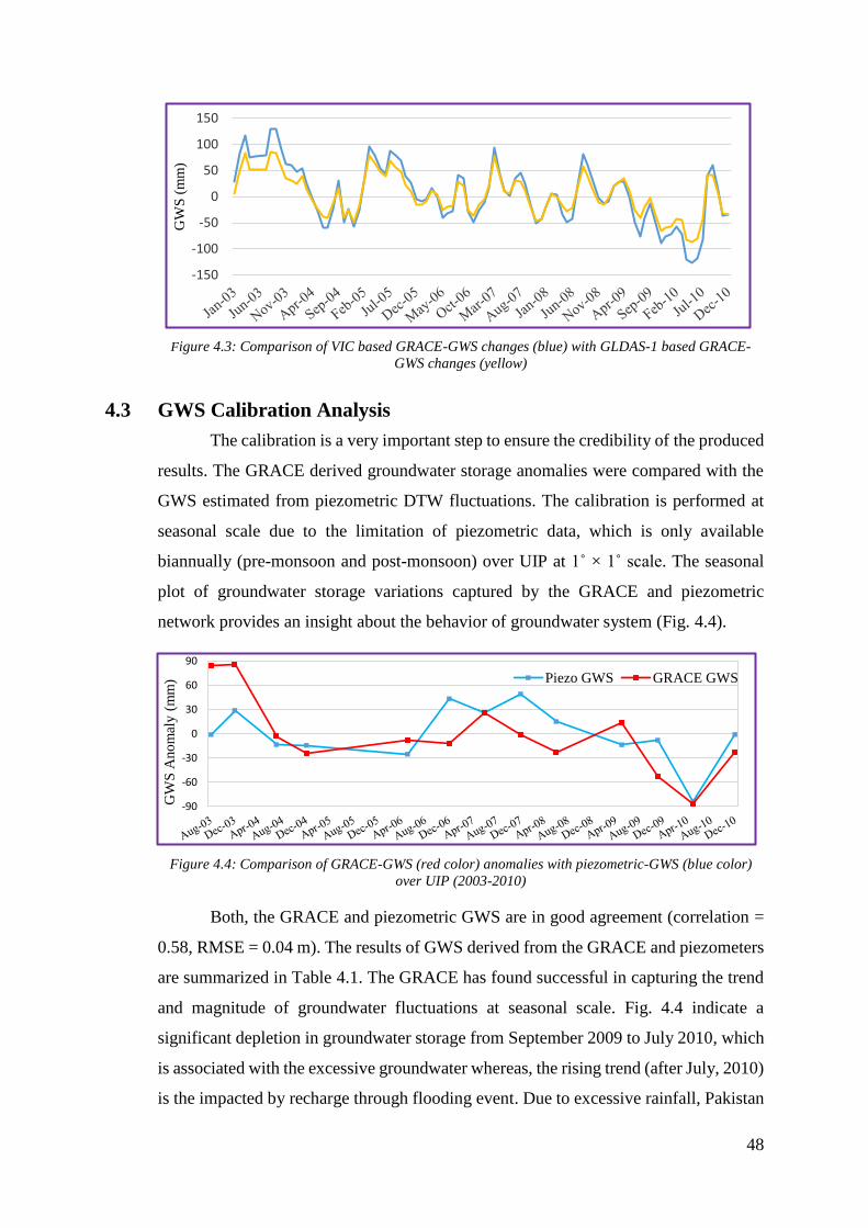
48
Figure 4.3: Comparison of VIC based GRACE-GWS changes (blue) with GLDAS-1 based GRACE-
GWS changes (yellow)
4.3 GWS Calibration Analysis
The calibration is a very important step to ensure the credibility of the produced
results. The GRACE derived groundwater storage anomalies were compared with the
GWS estimated from piezometric DTW fluctuations. The calibration is performed at
seasonal scale due to the limitation of piezometric data, which is only available
biannually (pre-monsoon and post-monsoon) over UIP at 1˚ × 1˚ scale. The seasonal
plot of groundwater storage variations captured by the GRACE and piezometric
network provides an insight about the behavior of groundwater system (Fig. 4.4).
Figure 4.4: Comparison of GRACE-GWS (red color) anomalies with piezometric-GWS (blue color)
over UIP (2003-2010)
Both, the GRACE and piezometric GWS are in good agreement (correlation =
0.58, RMSE = 0.04 m). The results of GWS derived from the GRACE and piezometers
are summarized in Table 4.1. The GRACE has found successful in capturing the trend
and magnitude of groundwater fluctuations at seasonal scale. Fig. 4.4 indicate a
significant depletion in groundwater storage from September 2009 to July 2010, which
is associated with the excessive groundwater whereas, the rising trend (after July, 2010)
is the impacted by recharge through flooding event. Due to excessive rainfall, Pakistan
-90
-60
-30
0
30
60
90
GW
S A
no
mal
y (
mm
) Piezo GWS GRACE GWS
-150
-100
-50
0
50
100
150
GW
S (
mm
)
49
was hit substantial flooding in August 2010. The GRACE has reported seasonal
groundwater storage depletion of about 1.48 km3 per year in comparison with
piezometers (0.39 km3 per year) from 2003-2010 over UIP (Table 4.1). One of the
possible reasons for this difference between data collection mechanism. The GRACE
observation is large aerial whereas the piezometric data is locally influenced point
observation. The local phenomenon such are recharge and neighboring pumping have
a direct impact on piezometric measurements. The inherent limitation of the GRACE
coarse spatial resolution is another reason for this different in depletion rates reported
by the GRACE and piezometers. Infect, the remote sensing is an indirect measure of
spatially average information collection of hydrological variables such as groundwater
storage. The accuracy of the GRACE increases with area coverage and it is more
accurate over large basins with ~200,000 km2 (Swenson et al. 2006). It is very important
to develop clear understanding about the mechanism of the GRACE data collection and
data processing process for the derivation of groundwater storage information. The
GRACE mission orbits the earth at an altitude of 450 km from the surface of earth and
records the variation in gravity induced by changes in density on or over the earth
surface. Despite of the fact that the GRACE is highly sensitive to even small changes
in gravity however, there are a number of factors, which impact the gravity signal in
the atmosphere and cause noises. Although, various filtering and signal restoration
techniques are used to improve the quality of total water storage anomaly, the
challenges are still there for further improvements. The simulation errors introduced by
hydrological models during the derivation of GWS from the GRACE-TWS is factor,
which impact to reduce the GRACE-GWS. So, indirect measurement of GWS from
space and piezometric measurement of water levels on the surface of earth are two
different mechanisms of data collection. These are infect two different quantities, which
are difficult to compare. The comparison with the results of groundwater modeling is
another discussion. Their accuracy is impacted due to input data limitations,
complexities of the groundwater system itself and climatic implications.
It is estimated that UIP has lost a stock of about 11.84 km3 fresh groundwater
storage in just 8 years of time (2003-2010) through extensive groundwater abstraction
for anthropogenic activities (Table 4.2). Figure 4.5 shows the variations in groundwater
stock over UIP during the study period. The projected scenario (2011-2014) indicates
a decreasing trend in groundwater stock, which highlights further loss of fresh
groundwater storage. This projected scenario is developed based on the relation

50
between TWS and GWS anomalies from 2003-2010. This trend is just indication about
the expected changes in groundwater stock, which may vary based on the inclusion of
actual data pertaining to model simulations from 2011-2014. In comparison with other
regional studies especially conducted in India subcontinent (Bhanja et al. 2017), the
results of current study also in an agreement referring to an overall trend of groundwater
depletion. However, only trends may be compared but not the depletion rates as these
vary from one area to another depending upon the patterns of groundwater recharge and
abstraction.
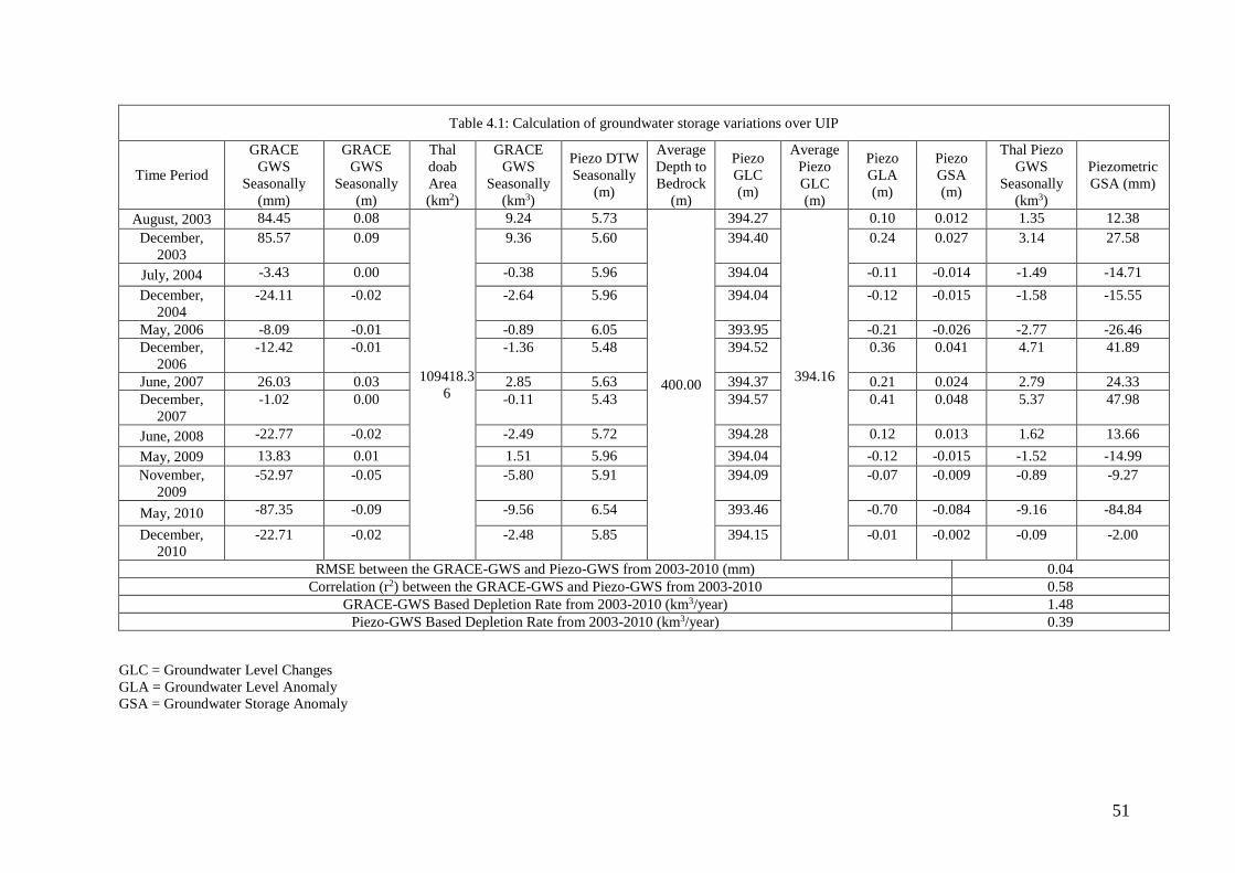
51
Table 4.1: Calculation of groundwater storage variations over UIP
Time Period
GRACE
GWS
Seasonally
(mm)
GRACE
GWS
Seasonally
(m)
Thal
doab
Area
(km2)
GRACE
GWS
Seasonally
(km3)
Piezo DTW
Seasonally
(m)
Average
Depth to
Bedrock
(m)
Piezo
GLC
(m)
Average
Piezo
GLC
(m)
Piezo
GLA
(m)
Piezo
GSA
(m)
Thal Piezo
GWS
Seasonally
(km3)
Piezometric
GSA (mm)
August, 2003 84.45 0.08
109418.3
6
9.24 5.73
400.00
394.27
394.16
0.10 0.012 1.35 12.38
December,
2003
85.57 0.09 9.36 5.60 394.40 0.24 0.027 3.14 27.58
July, 2004 -3.43 0.00 -0.38 5.96 394.04 -0.11 -0.014 -1.49 -14.71
December,
2004
-24.11 -0.02 -2.64 5.96 394.04 -0.12 -0.015 -1.58 -15.55
May, 2006 -8.09 -0.01 -0.89 6.05 393.95 -0.21 -0.026 -2.77 -26.46
December,
2006
-12.42 -0.01 -1.36 5.48 394.52 0.36 0.041 4.71 41.89
June, 2007 26.03 0.03 2.85 5.63 394.37 0.21 0.024 2.79 24.33
December,
2007
-1.02 0.00 -0.11 5.43 394.57 0.41 0.048 5.37 47.98
June, 2008 -22.77 -0.02 -2.49 5.72 394.28 0.12 0.013 1.62 13.66
May, 2009 13.83 0.01 1.51 5.96 394.04 -0.12 -0.015 -1.52 -14.99
November,
2009
-52.97 -0.05 -5.80 5.91 394.09 -0.07 -0.009 -0.89 -9.27
May, 2010 -87.35 -0.09 -9.56 6.54 393.46 -0.70 -0.084 -9.16 -84.84
December,
2010
-22.71 -0.02 -2.48 5.85 394.15 -0.01 -0.002 -0.09 -2.00
RMSE between the GRACE-GWS and Piezo-GWS from 2003-2010 (mm) 0.04
Correlation (r2) between the GRACE-GWS and Piezo-GWS from 2003-2010 0.58
GRACE-GWS Based Depletion Rate from 2003-2010 (km3/year) 1.48
Piezo-GWS Based Depletion Rate from 2003-2010 (km3/year) 0.39
GLC = Groundwater Level Changes
GLA = Groundwater Level Anomaly
GSA = Groundwater Storage Anomaly
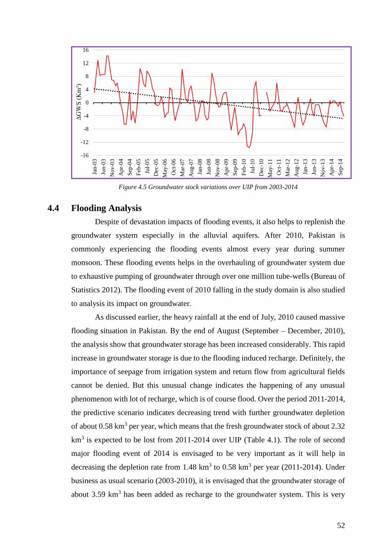
52
Figure 4.5 Groundwater stock variations over UIP from 2003-2014
4.4 Flooding Analysis
Despite of devastation impacts of flooding events, it also helps to replenish the
groundwater system especially in the alluvial aquifers. After 2010, Pakistan is
commonly experiencing the flooding events almost every year during summer
monsoon. These flooding events helps in the overhauling of groundwater system due
to exhaustive pumping of groundwater through over one million tube-wells (Bureau of
Statistics 2012). The flooding event of 2010 falling in the study domain is also studied
to analysis its impact on groundwater.
As discussed earlier, the heavy rainfall at the end of July, 2010 caused massive
flooding situation in Pakistan. By the end of August (September – December, 2010),
the analysis show that groundwater storage has been increased considerably. This rapid
increase in groundwater storage is due to the flooding induced recharge. Definitely, the
importance of seepage from irrigation system and return flow from agricultural fields
cannot be denied. But this unusual change indicates the happening of any unusual
phenomenon with lot of recharge, which is of course flood. Over the period 2011-2014,
the predictive scenario indicates decreasing trend with further groundwater depletion
of about 0.58 km3 per year, which means that the fresh groundwater stock of about 2.32
km3 is expected to be lost from 2011-2014 over UIP (Table 4.1). The role of second
major flooding event of 2014 is envisaged to be very important as it will help in
decreasing the depletion rate from 1.48 km3 to 0.58 km3 per year (2011-2014). Under
business as usual scenario (2003-2010), it is envisaged that the groundwater storage of
about 3.59 km3 has been added as recharge to the groundwater system. This is very
-16
-12
-8
-4
0
4
8
12
16
Jan
-03
Jun-0
3
No
v-0
3
Ap
r-04
Sep
-04
Feb
-05
Jul-
05
Dec
-05
May
-06
Oct
-06
Mar
-07
Au
g-0
7
Jan
-08
Jun-0
8
No
v-0
8
Ap
r-09
Sep
-09
Feb
-10
Jul-
10
Dec
-10
May
-11
Oct
-11
Mar
-12
Au
g-1
2
Jan
-13
Jun-1
3
No
v-1
3
Ap
r-14
Sep
-14
∆G
WS
(K
m³)
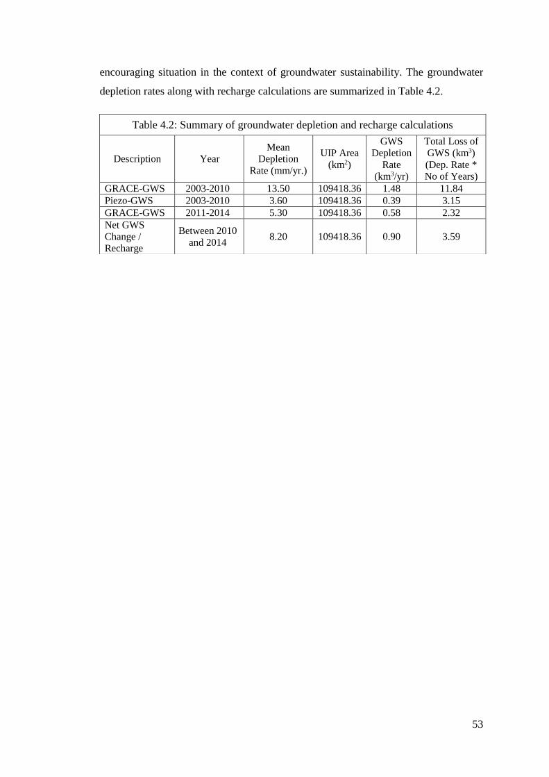
53
encouraging situation in the context of groundwater sustainability. The groundwater
depletion rates along with recharge calculations are summarized in Table 4.2.
Table 4.2: Summary of groundwater depletion and recharge calculations
Description Year
Mean
Depletion
Rate (mm/yr.)
UIP Area
(km2)
GWS
Depletion
Rate
(km3/yr)
Total Loss of
GWS (km3)
(Dep. Rate *
No of Years)
GRACE-GWS 2003-2010 13.50 109418.36 1.48 11.84
Piezo-GWS 2003-2010 3.60 109418.36 0.39 3.15
GRACE-GWS 2011-2014 5.30 109418.36 0.58 2.32
Net GWS
Change /
Recharge
Between 2010
and 2014 8.20 109418.36 0.90 3.59
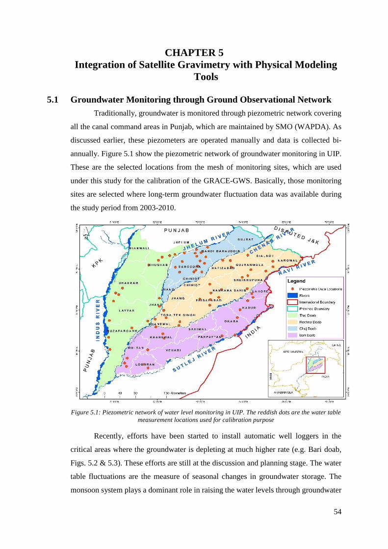
54
CHAPTER 5
Integration of Satellite Gravimetry with Physical Modeling
Tools
5.1 Groundwater Monitoring through Ground Observational Network
Traditionally, groundwater is monitored through piezometric network covering
all the canal command areas in Punjab, which are maintained by SMO (WAPDA). As
discussed earlier, these piezometers are operated manually and data is collected bi-
annually. Figure 5.1 show the piezometric network of groundwater monitoring in UIP.
These are the selected locations from the mesh of monitoring sites, which are used
under this study for the calibration of the GRACE-GWS. Basically, those monitoring
sites are selected where long-term groundwater fluctuation data was available during
the study period from 2003-2010.
Figure 5.1: Piezometric network of water level monitoring in UIP. The reddish dots are the water table
measurement locations used for calibration purpose
Recently, efforts have been started to install automatic well loggers in the
critical areas where the groundwater is depleting at much higher rate (e.g. Bari doab,
Figs. 5.2 & 5.3). These efforts are still at the discussion and planning stage. The water
table fluctuations are the measure of seasonal changes in groundwater storage. The
monsoon system plays a dominant role in raising the water levels through groundwater
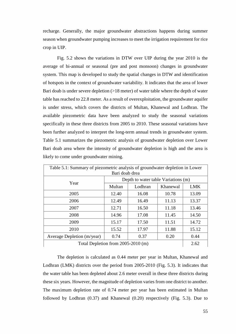
55
recharge. Generally, the major groundwater abstractions happens during summer
season when groundwater pumping increases to meet the irrigation requirement for rice
crop in UIP.
Fig. 5.2 shows the variations in DTW over UIP during the year 2010 is the
average of bi-annual or seasonal (pre and post monsoon) changes in groundwater
system. This map is developed to study the spatial changes in DTW and identification
of hotspots in the context of groundwater variability. It indicates that the area of lower
Bari doab is under severe depletion (>18 meter) of water table where the depth of water
table has reached to 22.8 meter. As a result of overexploitation, the groundwater aquifer
is under stress, which covers the districts of Multan, Khanewal and Lodhran. The
available piezometric data have been analyzed to study the seasonal variations
specifically in these three districts from 2005 to 2010. These seasonal variations have
been further analyzed to interpret the long-term annual trends in groundwater system.
Table 5.1 summarizes the piezometric analysis of groundwater depletion over Lower
Bari doab area where the intensity of groundwater depletion is high and the area is
likely to come under groundwater mining.
The depletion is calculated as 0.44 meter per year in Multan, Khanewal and
Lodhran (LMK) districts over the period from 2005-2010 (Fig. 5.3). It indicates that
the water table has been depleted about 2.6 meter overall in these three districts during
these six years. However, the magnitude of depletion varies from one district to another.
The maximum depletion rate of 0.74 meter per year has been estimated in Multan
followed by Lodhran (0.37) and Khanewal (0.20) respectively (Fig. 5.3). Due to
Table 5.1: Summary of piezometric analysis of groundwater depletion in Lower
Bari doab drea
Year Depth to water table Variations (m)
Multan Lodhran Khanewal LMK
2005 12.40 16.08 10.78 13.09
2006 12.49 16.49 11.13 13.37
2007 12.71 16.50 11.18 13.46
2008 14.96 17.08 11.45 14.50
2009 15.17 17.50 11.51 14.72
2010 15.52 17.97 11.88 15.12
Average Depletion (m/year) 0.74 0.37 0.20 0.44
Total Depletion from 2005-2010 (m) 2.62
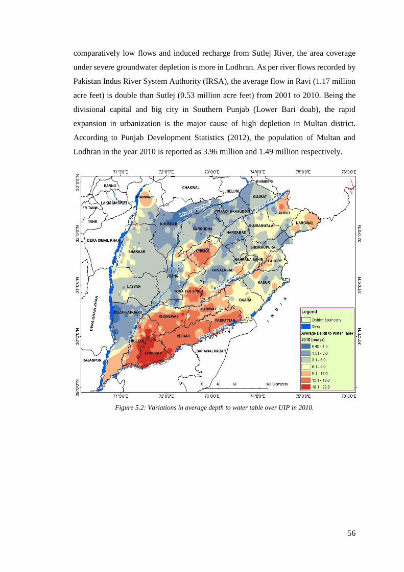
56
comparatively low flows and induced recharge from Sutlej River, the area coverage
under severe groundwater depletion is more in Lodhran. As per river flows recorded by
Pakistan Indus River System Authority (IRSA), the average flow in Ravi (1.17 million
acre feet) is double than Sutlej (0.53 million acre feet) from 2001 to 2010. Being the
divisional capital and big city in Southern Punjab (Lower Bari doab), the rapid
expansion in urbanization is the major cause of high depletion in Multan district.
According to Punjab Development Statistics (2012), the population of Multan and
Lodhran in the year 2010 is reported as 3.96 million and 1.49 million respectively.
Figure 5.2: Variations in average depth to water table over UIP in 2010.
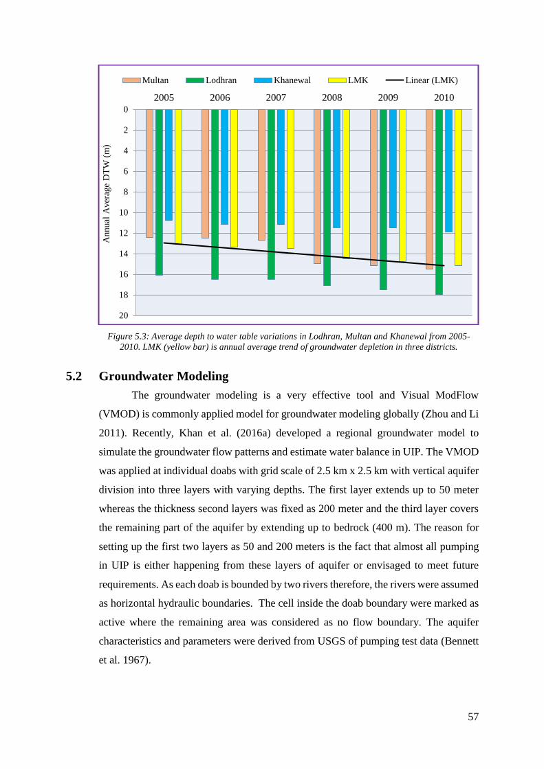
57
Figure 5.3: Average depth to water table variations in Lodhran, Multan and Khanewal from 2005-
2010. LMK (yellow bar) is annual average trend of groundwater depletion in three districts.
5.2 Groundwater Modeling
The groundwater modeling is a very effective tool and Visual ModFlow
(VMOD) is commonly applied model for groundwater modeling globally (Zhou and Li
2011). Recently, Khan et al. (2016a) developed a regional groundwater model to
simulate the groundwater flow patterns and estimate water balance in UIP. The VMOD
was applied at individual doabs with grid scale of 2.5 km x 2.5 km with vertical aquifer
division into three layers with varying depths. The first layer extends up to 50 meter
whereas the thickness second layers was fixed as 200 meter and the third layer covers
the remaining part of the aquifer by extending up to bedrock (400 m). The reason for
setting up the first two layers as 50 and 200 meters is the fact that almost all pumping
in UIP is either happening from these layers of aquifer or envisaged to meet future
requirements. As each doab is bounded by two rivers therefore, the rivers were assumed
as horizontal hydraulic boundaries. The cell inside the doab boundary were marked as
active where the remaining area was considered as no flow boundary. The aquifer
characteristics and parameters were derived from USGS of pumping test data (Bennett
et al. 1967).
0
2
4
6
8
10
12
14
16
18
20
2005 2006 2007 2008 2009 2010A
nnual
Aver
age
DT
W (
m)
Multan Lodhran Khanewal LMK Linear (LMK)
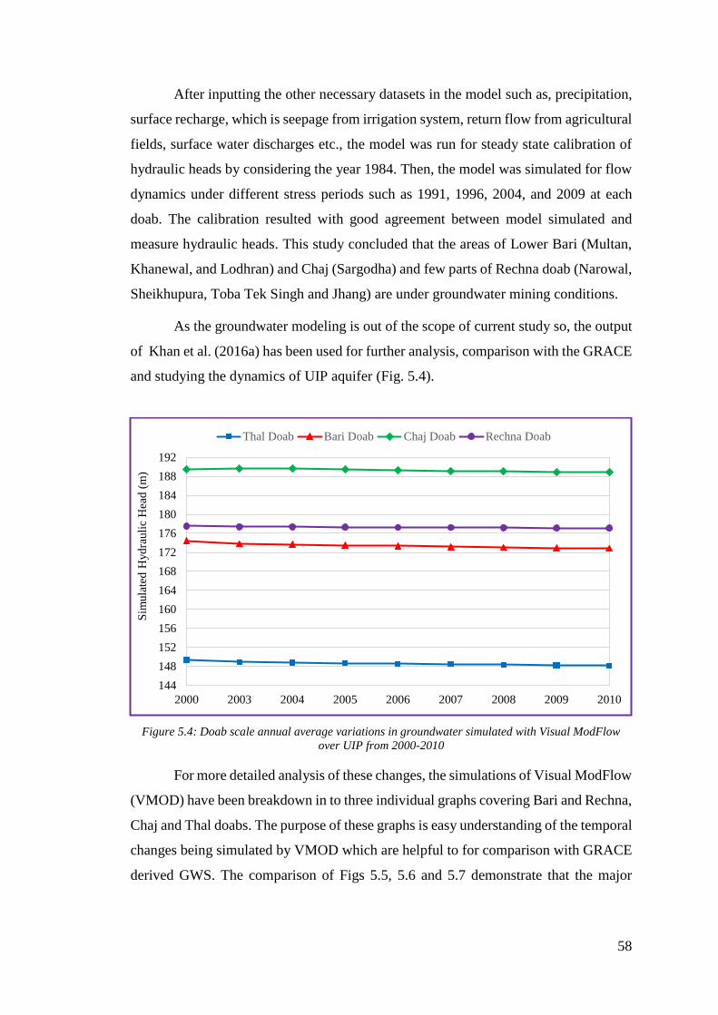
58
After inputting the other necessary datasets in the model such as, precipitation,
surface recharge, which is seepage from irrigation system, return flow from agricultural
fields, surface water discharges etc., the model was run for steady state calibration of
hydraulic heads by considering the year 1984. Then, the model was simulated for flow
dynamics under different stress periods such as 1991, 1996, 2004, and 2009 at each
doab. The calibration resulted with good agreement between model simulated and
measure hydraulic heads. This study concluded that the areas of Lower Bari (Multan,
Khanewal, and Lodhran) and Chaj (Sargodha) and few parts of Rechna doab (Narowal,
Sheikhupura, Toba Tek Singh and Jhang) are under groundwater mining conditions.
As the groundwater modeling is out of the scope of current study so, the output
of Khan et al. (2016a) has been used for further analysis, comparison with the GRACE
and studying the dynamics of UIP aquifer (Fig. 5.4).
Figure 5.4: Doab scale annual average variations in groundwater simulated with Visual ModFlow
over UIP from 2000-2010
For more detailed analysis of these changes, the simulations of Visual ModFlow
(VMOD) have been breakdown in to three individual graphs covering Bari and Rechna,
Chaj and Thal doabs. The purpose of these graphs is easy understanding of the temporal
changes being simulated by VMOD which are helpful to for comparison with GRACE
derived GWS. The comparison of Figs 5.5, 5.6 and 5.7 demonstrate that the major
144
148
152
156
160
164
168
172
176
180
184
188
192
2000 2003 2004 2005 2006 2007 2008 2009 2010
Sim
ula
ted
Hyd
rauli
c H
ead
(m
)
Thal Doab Bari Doab Chaj Doab Rechna Doab
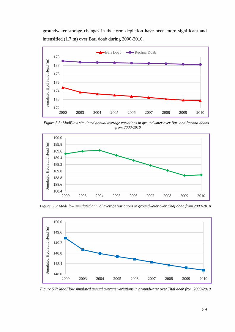
59
groundwater storage changes in the form depletion have been more significant and
intensified (1.7 m) over Bari doab during 2000-2010.
Figure 5.5: ModFlow simulated annual average variations in groundwater over Bari and Rechna doabs
from 2000-2010
Figure 5.6: ModFlow simulated annual average variations in groundwater over Chaj doab from 2000-2010
Figure 5.7: ModFlow simulated annual average variations in groundwater over Thal doab from 2000-2010
172
173
174
175
176
177
178
2000 2003 2004 2005 2006 2007 2008 2009 2010
Sim
ula
ted
Hyd
rauli
c H
ead
(m
)
Bari Doab Rechna Doab
188.4
188.6
188.8
189.0
189.2
189.4
189.6
189.8
190.0
2000 2003 2004 2005 2006 2007 2008 2009 2010
Sim
ula
ted
Hyd
rauli
c H
ead
(m
)
148.0
148.4
148.8
149.2
149.6
150.0
2000 2003 2004 2005 2006 2007 2008 2009 2010
Sim
ula
ted
Hyd
rauli
c H
ead
(m
)
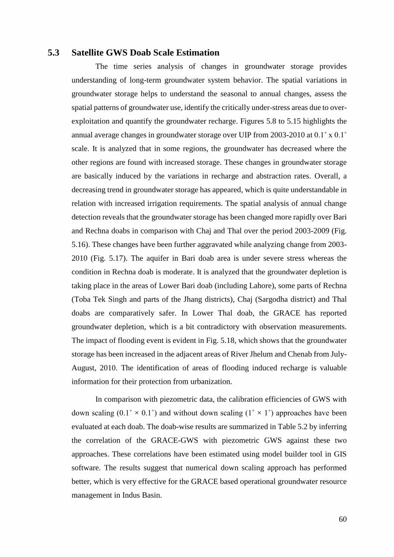
60
5.3 Satellite GWS Doab Scale Estimation
The time series analysis of changes in groundwater storage provides
understanding of long-term groundwater system behavior. The spatial variations in
groundwater storage helps to understand the seasonal to annual changes, assess the
spatial patterns of groundwater use, identify the critically under-stress areas due to over-
exploitation and quantify the groundwater recharge. Figures 5.8 to 5.15 highlights the
annual average changes in groundwater storage over UIP from 2003-2010 at 0.1˚ x 0.1˚
scale. It is analyzed that in some regions, the groundwater has decreased where the
other regions are found with increased storage. These changes in groundwater storage
are basically induced by the variations in recharge and abstraction rates. Overall, a
decreasing trend in groundwater storage has appeared, which is quite understandable in
relation with increased irrigation requirements. The spatial analysis of annual change
detection reveals that the groundwater storage has been changed more rapidly over Bari
and Rechna doabs in comparison with Chaj and Thal over the period 2003-2009 (Fig.
5.16). These changes have been further aggravated while analyzing change from 2003-
2010 (Fig. 5.17). The aquifer in Bari doab area is under severe stress whereas the
condition in Rechna doab is moderate. It is analyzed that the groundwater depletion is
taking place in the areas of Lower Bari doab (including Lahore), some parts of Rechna
(Toba Tek Singh and parts of the Jhang districts), Chaj (Sargodha district) and Thal
doabs are comparatively safer. In Lower Thal doab, the GRACE has reported
groundwater depletion, which is a bit contradictory with observation measurements.
The impact of flooding event is evident in Fig. 5.18, which shows that the groundwater
storage has been increased in the adjacent areas of River Jhelum and Chenab from July-
August, 2010. The identification of areas of flooding induced recharge is valuable
information for their protection from urbanization.
In comparison with piezometric data, the calibration efficiencies of GWS with
down scaling (0.1˚ × 0.1˚) and without down scaling (1˚ × 1˚) approaches have been
evaluated at each doab. The doab-wise results are summarized in Table 5.2 by inferring
the correlation of the GRACE-GWS with piezometric GWS against these two
approaches. These correlations have been estimated using model builder tool in GIS
software. The results suggest that numerical down scaling approach has performed
better, which is very effective for the GRACE based operational groundwater resource
management in Indus Basin.
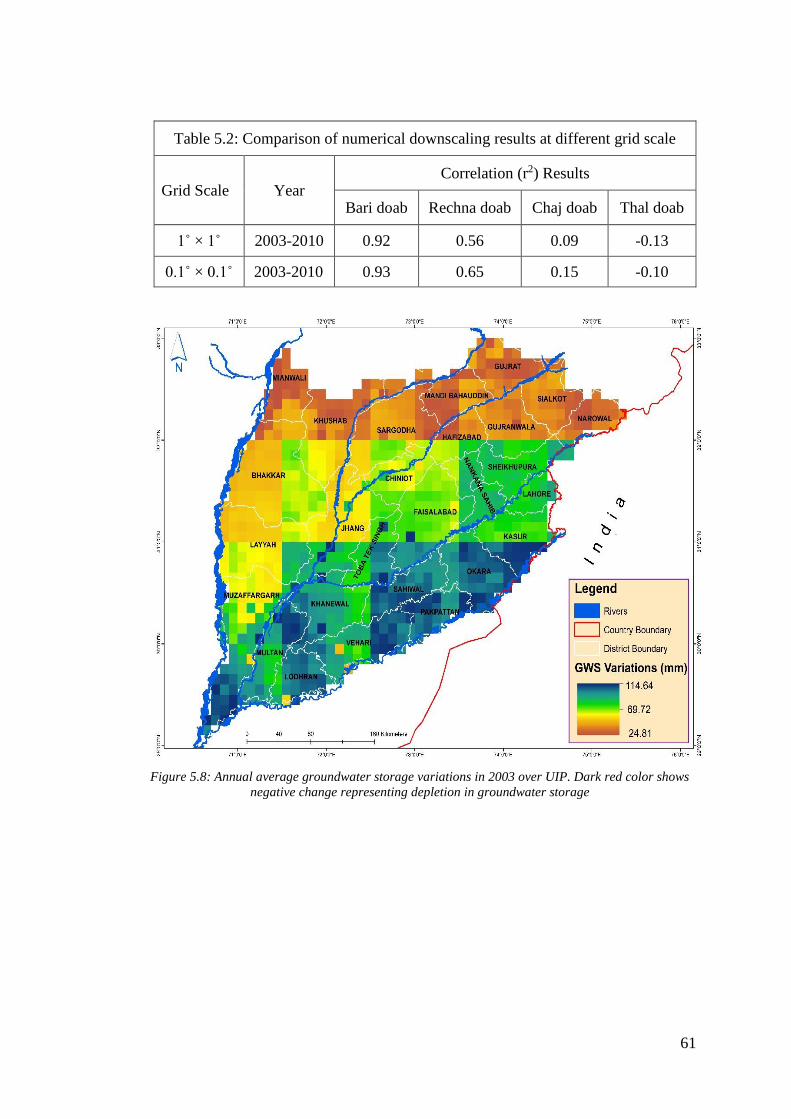
61
Table 5.2: Comparison of numerical downscaling results at different grid scale
Grid Scale Year Correlation (r2) Results
Bari doab Rechna doab Chaj doab Thal doab
1˚ × 1˚ 2003-2010 0.92 0.56 0.09 -0.13
0.1˚ × 0.1˚ 2003-2010 0.93 0.65 0.15 -0.10
Figure 5.8: Annual average groundwater storage variations in 2003 over UIP. Dark red color shows
negative change representing depletion in groundwater storage
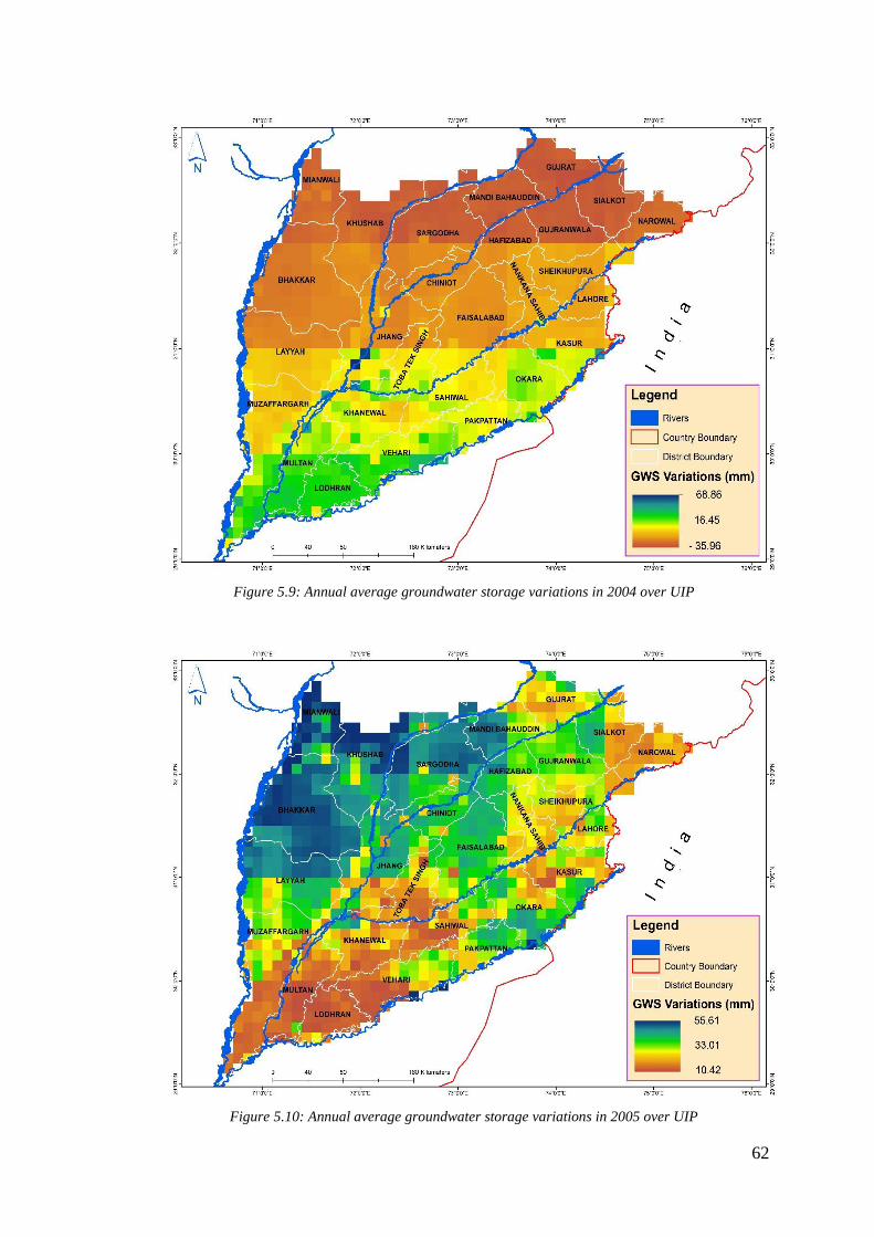
62
Figure 5.9: Annual average groundwater storage variations in 2004 over UIP
Figure 5.10: Annual average groundwater storage variations in 2005 over UIP
63
Figure 5.11: Annual average groundwater storage variations in 2006 over UIP
Figure 5.12: Annual average groundwater storage variations in 2007 over UIP
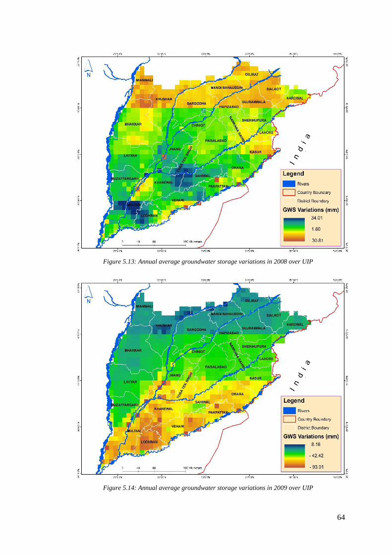
64
Figure 5.13: Annual average groundwater storage variations in 2008 over UIP
Figure 5.14: Annual average groundwater storage variations in 2009 over UIP
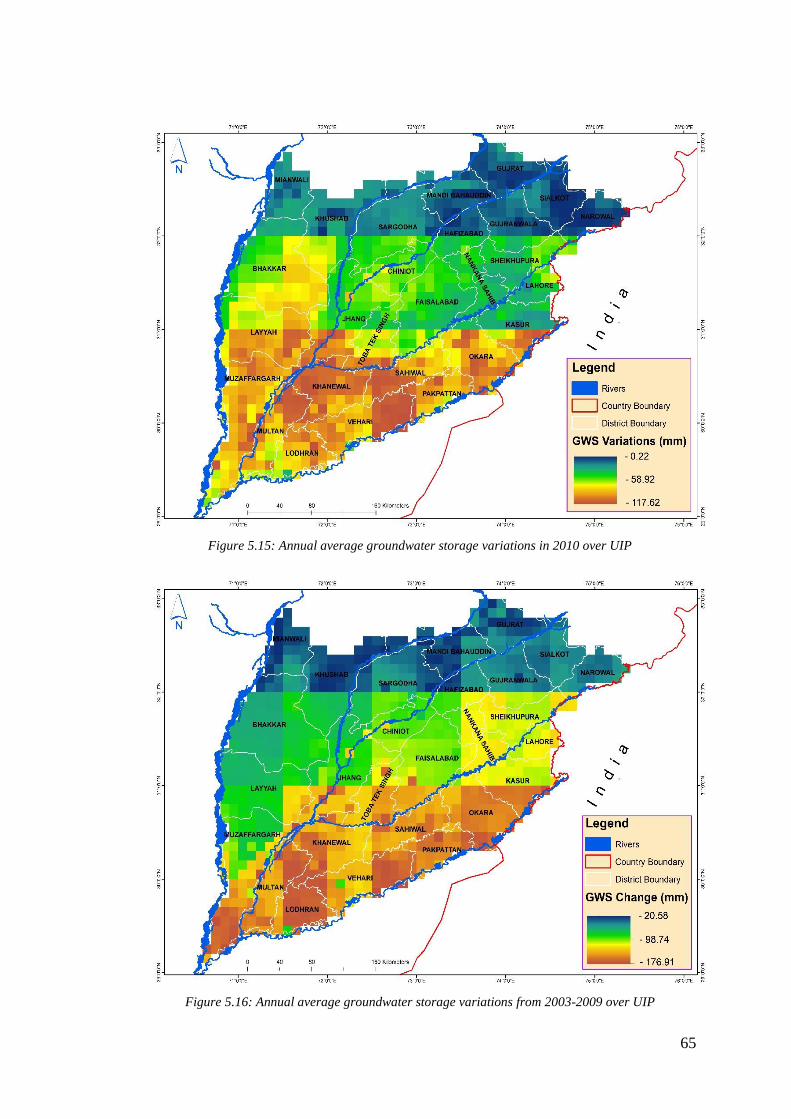
65
Figure 5.15: Annual average groundwater storage variations in 2010 over UIP
Figure 5.16: Annual average groundwater storage variations from 2003-2009 over UIP
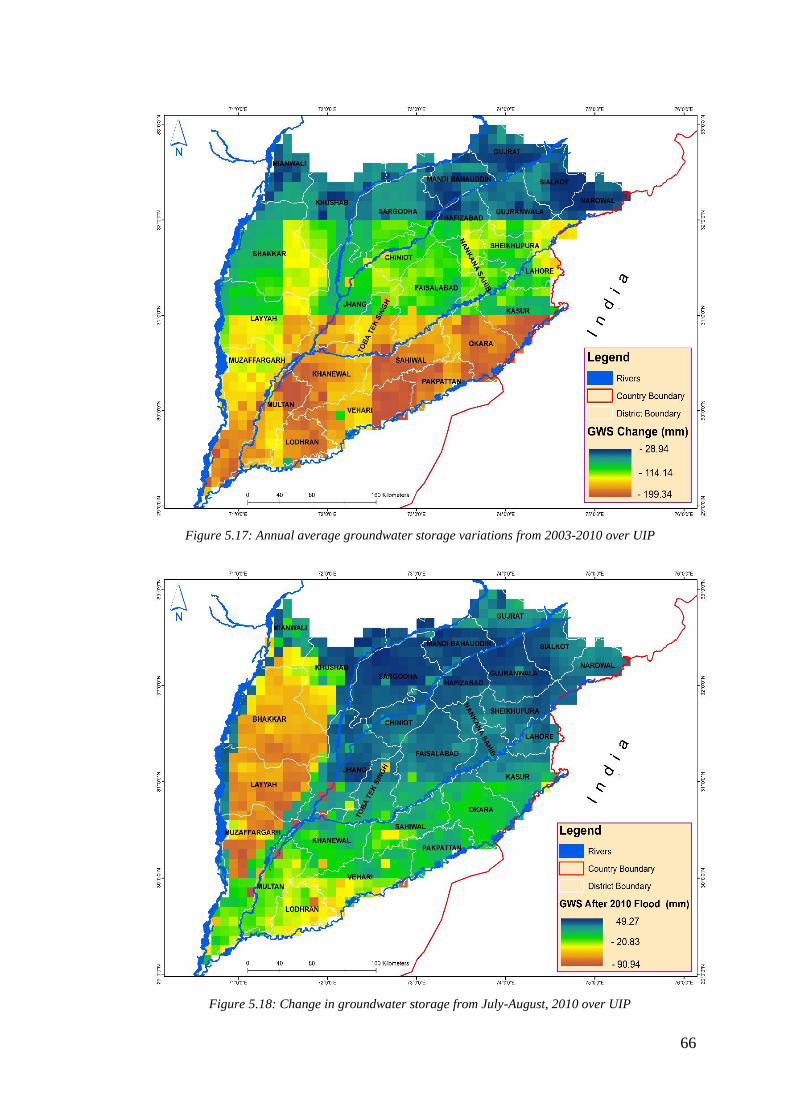
66
Figure 5.17: Annual average groundwater storage variations from 2003-2010 over UIP
Figure 5.18: Change in groundwater storage from July-August, 2010 over UIP
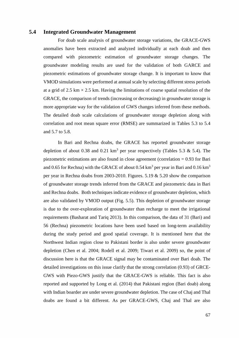
67
5.4 Integrated Groundwater Management
For doab scale analysis of groundwater storage variations, the GRACE-GWS
anomalies have been extracted and analyzed individually at each doab and then
compared with piezometric estimation of groundwater storage changes. The
groundwater modeling results are used for the validation of both GARCE and
piezometric estimations of groundwater storage change. It is important to know that
VMOD simulations were performed at annual scale by selecting different stress periods
at a grid of 2.5 km × 2.5 km. Having the limitations of coarse spatial resolution of the
GRACE, the comparison of trends (increasing or decreasing) in groundwater storage is
more appropriate way for the validation of GWS changes inferred from these methods.
The detailed doab scale calculations of groundwater storage depletion along with
correlation and root mean square error (RMSE) are summarized in Tables 5.3 to 5.4
and 5.7 to 5.8.
In Bari and Rechna doabs, the GRACE has reported groundwater storage
depletion of about 0.38 and 0.21 km3 per year respectively (Tables 5.3 & 5.4). The
piezometric estimations are also found in close agreement (correlation = 0.93 for Bari
and 0.65 for Rechna) with the GRACE of about 0.54 km3 per year in Bari and 0.16 km3
per year in Rechna doabs from 2003-2010. Figures. 5.19 & 5.20 show the comparison
of groundwater storage trends inferred from the GRACE and piezometric data in Bari
and Rechna doabs. Both techniques indicate evidence of groundwater depletion, which
are also validated by VMOD output (Fig. 5.5). This depletion of groundwater storage
is due to the over-exploration of groundwater than recharge to meet the irrigational
requirements (Basharat and Tariq 2013). In this comparison, the data of 31 (Bari) and
56 (Rechna) piezometric locations have been used based on long-term availability
during the study period and good spatial coverage. It is mentioned here that the
Northwest Indian region close to Pakistani border is also under severe groundwater
depletion (Chen et al. 2004; Rodell et al. 2009; Tiwari et al. 2009) so, the point of
discussion here is that the GRACE signal may be contaminated over Bari doab. The
detailed investigations on this issue clarify that the strong correlation (0.93) of GRCE-
GWS with Piezo-GWS justify that the GRACE-GWS is reliable. This fact is also
reported and supported by Long et al. (2014) that Pakistani region (Bari doab) along
with Indian boarder are under severe groundwater depletion. The case of Chaj and Thal
doabs are found a bit different. As per GRACE-GWS, Chaj and Thal are also
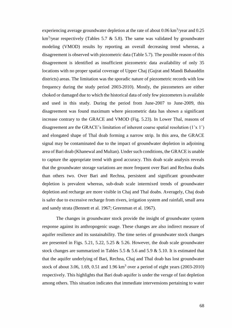
68
experiencing average groundwater depletion at the rate of about 0.06 km3/year and 0.25
km3/year respectively (Tables 5.7 & 5.8). The same was validated by groundwater
modeling (VMOD) results by reporting an overall decreasing trend whereas, a
disagreement is observed with piezometric data (Table 5.7). The possible reason of this
disagreement is identified as insufficient piezometric data availability of only 35
locations with no proper spatial coverage of Upper Chaj (Gujrat and Mandi Bahauddin
districts) areas. The limitation was the sporadic nature of piezometric records with low
frequency during the study period 2003-2010). Mostly, the piezometers are either
choked or damaged due to which the historical data of only few piezometers is available
and used in this study. During the period from June-2007 to June-2009, this
disagreement was found maximum where piezometric data has shown a significant
increase contrary to the GRACE and VMOD (Fig. 5.23). In Lower Thal, reasons of
disagreement are the GRACE’s limitation of inherent coarse spatial resolution (1˚x 1˚)
and elongated shape of Thal doab forming a narrow strip. In this area, the GRACE
signal may be contaminated due to the impact of groundwater depletion in adjoining
area of Bari doab (Khanewal and Multan). Under such conditions, the GRACE is unable
to capture the appropriate trend with good accuracy. This doab scale analysis reveals
that the groundwater storage variations are more frequent over Bari and Rechna doabs
than others two. Over Bari and Rechna, persistent and significant groundwater
depletion is prevalent whereas, sub-doab scale intermixed trends of groundwater
depletion and recharge are more visible in Chaj and Thal doabs. Averagely, Chaj doab
is safer due to excessive recharge from rivers, irrigation system and rainfall, small area
and sandy strata (Bennett et al. 1967; Greenman et al. 1967).
The changes in groundwater stock provide the insight of groundwater system
response against its anthropogenic usage. These changes are also indirect measure of
aquifer resilience and its sustainability. The time series of groundwater stock changes
are presented in Figs. 5.21, 5.22, 5.25 & 5.26. However, the doab scale groundwater
stock changes are summarized in Tables 5.5 & 5.6 and 5.9 & 5.10. It is estimated that
that the aquifer underlying of Bari, Rechna, Chaj and Thal doab has lost groundwater
stock of about 3.06, 1.69, 0.51 and 1.96 km3 over a period of eight years (2003-2010)
respectively. This highlights that Bari doab aquifer is under the versge of fast depletion
among others. This situation indicates that immediate intervensions pertaining to water
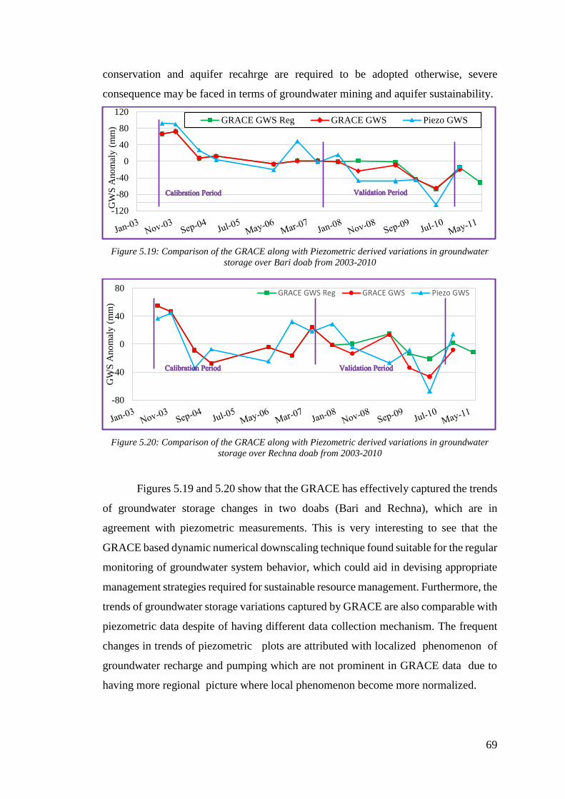
69
conservation and aquifer recahrge are required to be adopted otherwise, severe
consequence may be faced in terms of groundwater mining and aquifer sustainability.
Figure 5.19: Comparison of the GRACE along with Piezometric derived variations in groundwater
storage over Bari doab from 2003-2010
Figure 5.20: Comparison of the GRACE along with Piezometric derived variations in groundwater
storage over Rechna doab from 2003-2010
Figures 5.19 and 5.20 show that the GRACE has effectively captured the trends
of groundwater storage changes in two doabs (Bari and Rechna), which are in
agreement with piezometric measurements. This is very interesting to see that the
GRACE based dynamic numerical downscaling technique found suitable for the regular
monitoring of groundwater system behavior, which could aid in devising appropriate
management strategies required for sustainable resource management. Furthermore, the
trends of groundwater storage variations captured by GRACE are also comparable with
piezometric data despite of having different data collection mechanism. The frequent
changes in trends of piezometric plots are attributed with localized phenomenon of
groundwater recharge and pumping which are not prominent in GRACE data due to
having more regional picture where local phenomenon become more normalized.
-120
-80
-40
0
40
80
120G
WS
Ano
mal
y (
mm
)GRACE GWS Reg GRACE GWS Piezo GWS
-80
-40
0
40
80
GW
S A
no
mal
y (
mm
)
GRACE GWS Reg GRACE GWS Piezo GWS
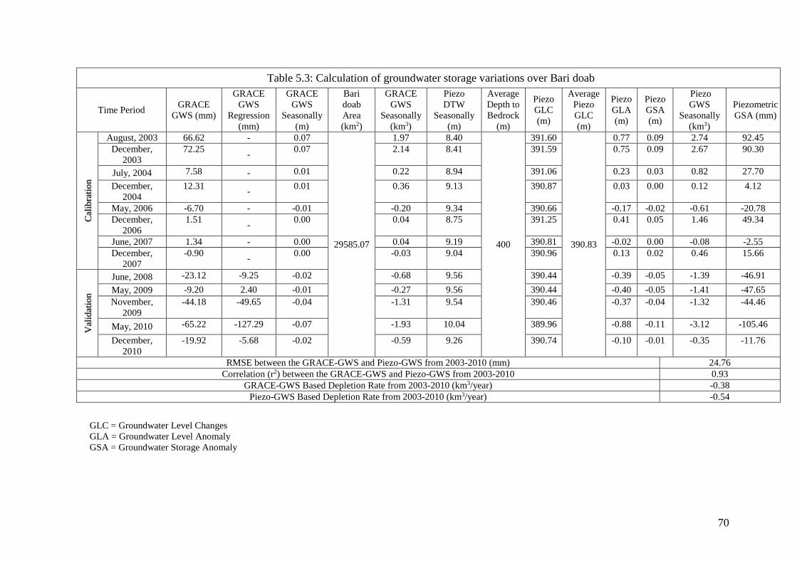
70
Table 5.3: Calculation of groundwater storage variations over Bari doab
Time Period GRACE
GWS (mm)
GRACE
GWS
Regression
(mm)
GRACE
GWS
Seasonally
(m)
Bari
doab
Area
(km2)
GRACE
GWS
Seasonally
(km3)
Piezo
DTW
Seasonally
(m)
Average
Depth to
Bedrock
(m)
Piezo
GLC
(m)
Average
Piezo
GLC
(m)
Piezo
GLA
(m)
Piezo
GSA
(m)
Piezo
GWS
Seasonally
(km3)
Piezometric
GSA (mm)
Cal
ibra
tio
n
August, 2003 66.62 - 0.07
29585.07
1.97 8.40
400
391.60
390.83
0.77 0.09 2.74 92.45
December,
2003
72.25 -
0.07 2.14 8.41 391.59 0.75 0.09 2.67 90.30
July, 2004 7.58 - 0.01 0.22 8.94 391.06 0.23 0.03 0.82 27.70
December,
2004
12.31 -
0.01 0.36 9.13 390.87 0.03 0.00 0.12 4.12
May, 2006 -6.70 - -0.01 -0.20 9.34 390.66 -0.17 -0.02 -0.61 -20.78
December,
2006
1.51 -
0.00 0.04 8.75 391.25 0.41 0.05 1.46 49.34
June, 2007 1.34 - 0.00 0.04 9.19 390.81 -0.02 0.00 -0.08 -2.55
December,
2007
-0.90 -
0.00 -0.03 9.04 390.96 0.13 0.02 0.46 15.66
Val
idat
ion
June, 2008 -23.12 -9.25 -0.02 -0.68 9.56 390.44 -0.39 -0.05 -1.39 -46.91
May, 2009 -9.20 2.40 -0.01 -0.27 9.56 390.44 -0.40 -0.05 -1.41 -47.65
November,
2009
-44.18 -49.65 -0.04 -1.31 9.54 390.46 -0.37 -0.04 -1.32 -44.46
May, 2010 -65.22 -127.29 -0.07 -1.93 10.04 389.96 -0.88 -0.11 -3.12 -105.46
December,
2010
-19.92 -5.68 -0.02 -0.59 9.26 390.74 -0.10 -0.01 -0.35 -11.76
RMSE between the GRACE-GWS and Piezo-GWS from 2003-2010 (mm) 24.76
Correlation (r2) between the GRACE-GWS and Piezo-GWS from 2003-2010 0.93
GRACE-GWS Based Depletion Rate from 2003-2010 (km3/year) -0.38
Piezo-GWS Based Depletion Rate from 2003-2010 (km3/year) -0.54
GLC = Groundwater Level Changes
GLA = Groundwater Level Anomaly
GSA = Groundwater Storage Anomaly
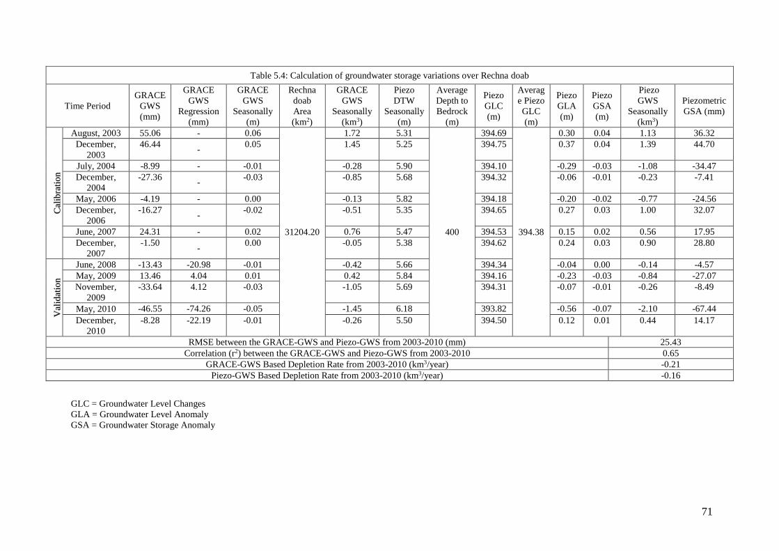
71
Table 5.4: Calculation of groundwater storage variations over Rechna doab
Time Period
GRACE
GWS
(mm)
GRACE
GWS
Regression
(mm)
GRACE
GWS
Seasonally
(m)
Rechna
doab
Area
(km2)
GRACE
GWS
Seasonally
(km3)
Piezo
DTW
Seasonally
(m)
Average
Depth to
Bedrock
(m)
Piezo
GLC
(m)
Averag
e Piezo
GLC
(m)
Piezo
GLA
(m)
Piezo
GSA
(m)
Piezo
GWS
Seasonally
(km3)
Piezometric
GSA (mm)
Cal
ibra
tio
n
August, 2003 55.06 - 0.06
31204.20
1.72 5.31
400
394.69
394.38
0.30 0.04 1.13 36.32
December,
2003
46.44 -
0.05 1.45 5.25 394.75 0.37 0.04 1.39 44.70
July, 2004 -8.99 - -0.01 -0.28 5.90 394.10 -0.29 -0.03 -1.08 -34.47
December,
2004
-27.36 -
-0.03 -0.85 5.68 394.32 -0.06 -0.01 -0.23 -7.41
May, 2006 -4.19 - 0.00 -0.13 5.82 394.18 -0.20 -0.02 -0.77 -24.56
December,
2006
-16.27 -
-0.02 -0.51 5.35 394.65 0.27 0.03 1.00 32.07
June, 2007 24.31 - 0.02 0.76 5.47 394.53 0.15 0.02 0.56 17.95
December,
2007
-1.50 -
0.00 -0.05 5.38 394.62 0.24 0.03 0.90 28.80
Val
idat
ion
June, 2008 -13.43 -20.98 -0.01 -0.42 5.66 394.34 -0.04 0.00 -0.14 -4.57
May, 2009 13.46 4.04 0.01 0.42 5.84 394.16 -0.23 -0.03 -0.84 -27.07
November,
2009
-33.64 4.12 -0.03 -1.05 5.69 394.31 -0.07 -0.01 -0.26 -8.49
May, 2010 -46.55 -74.26 -0.05 -1.45 6.18 393.82 -0.56 -0.07 -2.10 -67.44
December,
2010
-8.28 -22.19 -0.01 -0.26 5.50 394.50 0.12 0.01 0.44 14.17
RMSE between the GRACE-GWS and Piezo-GWS from 2003-2010 (mm) 25.43
Correlation (r2) between the GRACE-GWS and Piezo-GWS from 2003-2010 0.65
GRACE-GWS Based Depletion Rate from 2003-2010 (km3/year) -0.21
Piezo-GWS Based Depletion Rate from 2003-2010 (km3/year) -0.16
GLC = Groundwater Level Changes
GLA = Groundwater Level Anomaly
GSA = Groundwater Storage Anomaly
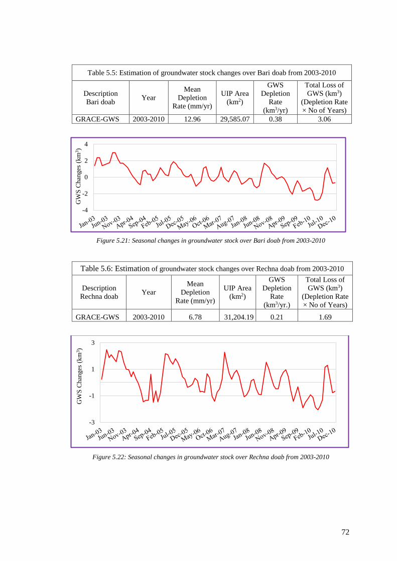
72
Table 5.5: Estimation of groundwater stock changes over Bari doab from 2003-2010
Description
Bari doab Year
Mean
Depletion
Rate (mm/yr)
UIP Area
(km2)
GWS
Depletion
Rate
(km3/yr)
Total Loss of
GWS (km3)
(Depletion Rate
× No of Years)
GRACE-GWS 2003-2010 12.96 29,585.07 0.38 3.06
Figure 5.21: Seasonal changes in groundwater stock over Bari doab from 2003-2010
Table 5.6: Estimation of groundwater stock changes over Rechna doab from 2003-2010
Description
Rechna doab Year
Mean
Depletion
Rate (mm/yr)
UIP Area
(km2)
GWS
Depletion
Rate
(km3/yr.)
Total Loss of
GWS (km3)
(Depletion Rate
× No of Years)
GRACE-GWS 2003-2010 6.78 31,204.19 0.21 1.69
Figure 5.22: Seasonal changes in groundwater stock over Rechna doab from 2003-2010
-3
-1
1
3
GW
S C
han
ges
(km
3)
-4
-2
0
2
4
GW
S C
han
ges
(km
3)
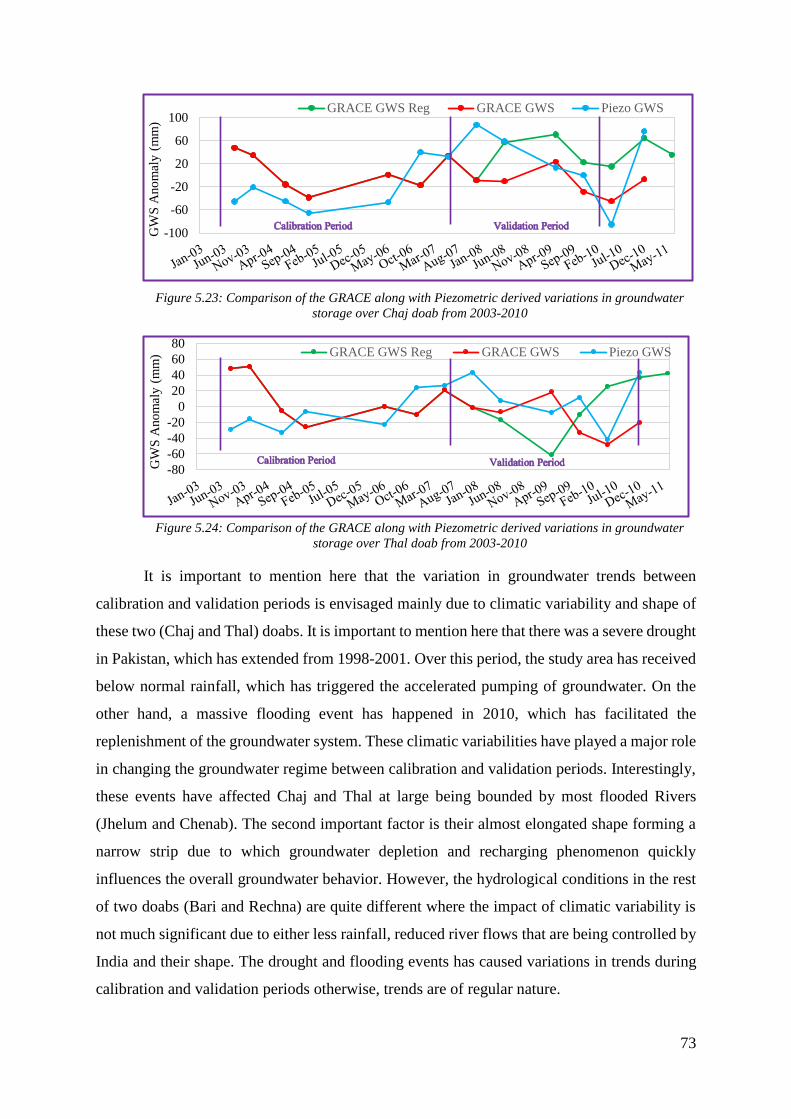
73
Figure 5.23: Comparison of the GRACE along with Piezometric derived variations in groundwater
storage over Chaj doab from 2003-2010
Figure 5.24: Comparison of the GRACE along with Piezometric derived variations in groundwater
storage over Thal doab from 2003-2010
It is important to mention here that the variation in groundwater trends between
calibration and validation periods is envisaged mainly due to climatic variability and shape of
these two (Chaj and Thal) doabs. It is important to mention here that there was a severe drought
in Pakistan, which has extended from 1998-2001. Over this period, the study area has received
below normal rainfall, which has triggered the accelerated pumping of groundwater. On the
other hand, a massive flooding event has happened in 2010, which has facilitated the
replenishment of the groundwater system. These climatic variabilities have played a major role
in changing the groundwater regime between calibration and validation periods. Interestingly,
these events have affected Chaj and Thal at large being bounded by most flooded Rivers
(Jhelum and Chenab). The second important factor is their almost elongated shape forming a
narrow strip due to which groundwater depletion and recharging phenomenon quickly
influences the overall groundwater behavior. However, the hydrological conditions in the rest
of two doabs (Bari and Rechna) are quite different where the impact of climatic variability is
not much significant due to either less rainfall, reduced river flows that are being controlled by
India and their shape. The drought and flooding events has caused variations in trends during
calibration and validation periods otherwise, trends are of regular nature.
-100
-60
-20
20
60
100
GW
S A
no
mal
y (
mm
)
GRACE GWS Reg GRACE GWS Piezo GWS
-80
-60
-40
-20
0
20
40
60
80
GW
S A
no
mal
y (
mm
) GRACE GWS Reg GRACE GWS Piezo GWS
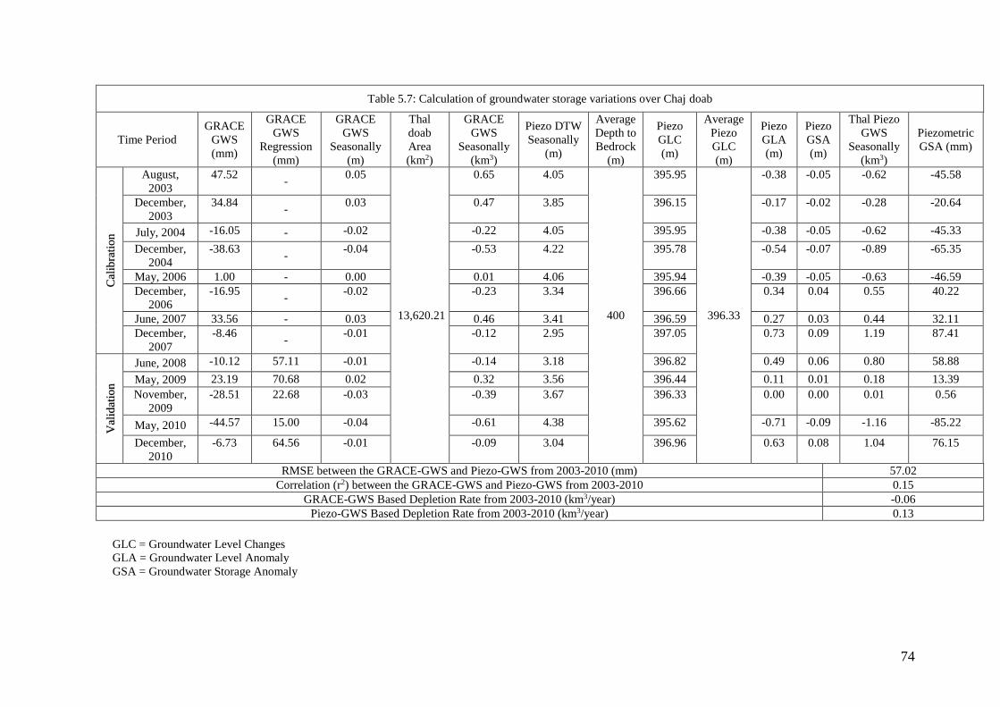
74
Table 5.7: Calculation of groundwater storage variations over Chaj doab
Time Period
GRACE
GWS
(mm)
GRACE
GWS
Regression
(mm)
GRACE
GWS
Seasonally
(m)
Thal
doab
Area
(km2)
GRACE
GWS
Seasonally
(km3)
Piezo DTW
Seasonally
(m)
Average
Depth to
Bedrock
(m)
Piezo
GLC
(m)
Average
Piezo
GLC
(m)
Piezo
GLA
(m)
Piezo
GSA
(m)
Thal Piezo
GWS
Seasonally
(km3)
Piezometric
GSA (mm)
Cal
ibra
tio
n
August,
2003
47.52 -
0.05
13,620.21
0.65 4.05
400
395.95
396.33
-0.38 -0.05 -0.62 -45.58
December,
2003
34.84 -
0.03 0.47 3.85 396.15 -0.17 -0.02 -0.28 -20.64
July, 2004 -16.05 - -0.02 -0.22 4.05 395.95 -0.38 -0.05 -0.62 -45.33
December,
2004
-38.63 -
-0.04 -0.53 4.22 395.78 -0.54 -0.07 -0.89 -65.35
May, 2006 1.00 - 0.00 0.01 4.06 395.94 -0.39 -0.05 -0.63 -46.59
December,
2006
-16.95 -
-0.02 -0.23 3.34 396.66 0.34 0.04 0.55 40.22
June, 2007 33.56 - 0.03 0.46 3.41 396.59 0.27 0.03 0.44 32.11
December,
2007
-8.46 -
-0.01 -0.12 2.95 397.05 0.73 0.09 1.19 87.41
Val
idat
ion
June, 2008 -10.12 57.11 -0.01 -0.14 3.18 396.82 0.49 0.06 0.80 58.88
May, 2009 23.19 70.68 0.02 0.32 3.56 396.44 0.11 0.01 0.18 13.39
November,
2009
-28.51 22.68 -0.03 -0.39 3.67 396.33 0.00 0.00 0.01 0.56
May, 2010 -44.57 15.00 -0.04 -0.61 4.38 395.62 -0.71 -0.09 -1.16 -85.22
December,
2010
-6.73 64.56 -0.01 -0.09 3.04 396.96 0.63 0.08 1.04 76.15
RMSE between the GRACE-GWS and Piezo-GWS from 2003-2010 (mm) 57.02
Correlation (r2) between the GRACE-GWS and Piezo-GWS from 2003-2010 0.15
GRACE-GWS Based Depletion Rate from 2003-2010 (km3/year) -0.06
Piezo-GWS Based Depletion Rate from 2003-2010 (km3/year) 0.13
GLC = Groundwater Level Changes
GLA = Groundwater Level Anomaly
GSA = Groundwater Storage Anomaly
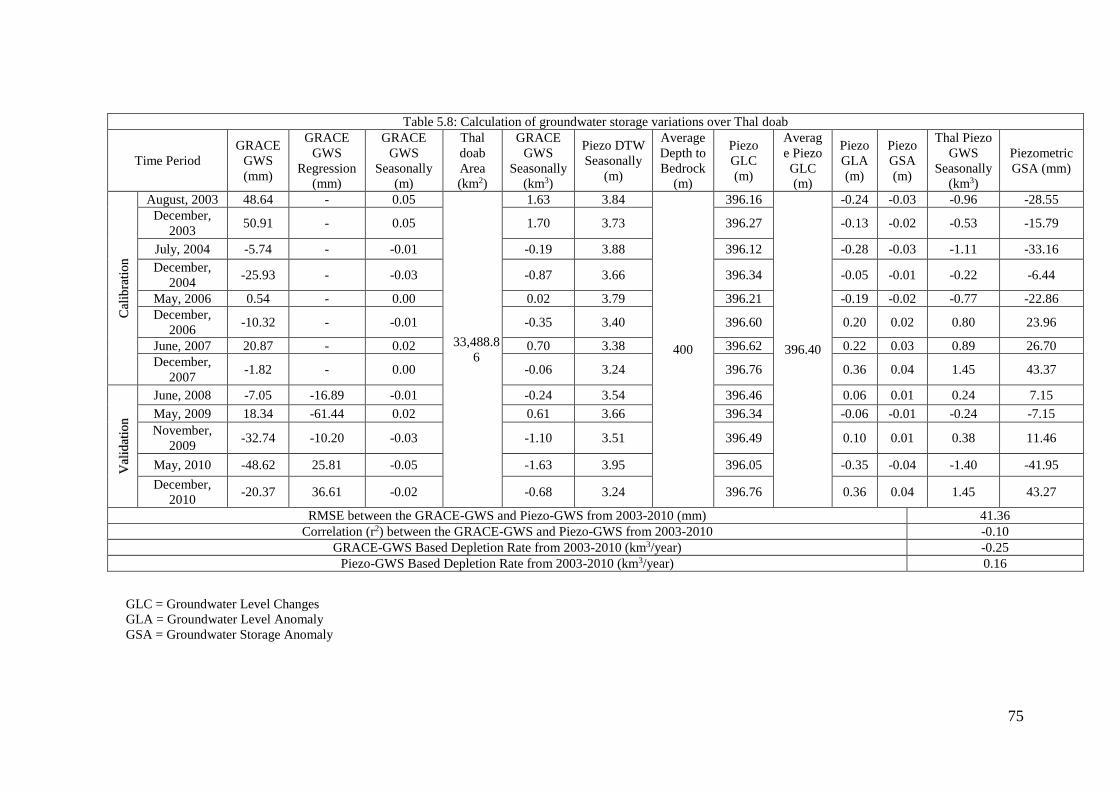
75
Table 5.8: Calculation of groundwater storage variations over Thal doab
Time Period
GRACE
GWS
(mm)
GRACE
GWS
Regression
(mm)
GRACE
GWS
Seasonally
(m)
Thal
doab
Area
(km2)
GRACE
GWS
Seasonally
(km3)
Piezo DTW
Seasonally
(m)
Average
Depth to
Bedrock
(m)
Piezo
GLC
(m)
Averag
e Piezo
GLC
(m)
Piezo
GLA
(m)
Piezo
GSA
(m)
Thal Piezo
GWS
Seasonally
(km3)
Piezometric
GSA (mm)
Cal
ibra
tio
n
August, 2003 48.64 - 0.05
33,488.8
6
1.63 3.84
400
396.16
396.40
-0.24 -0.03 -0.96 -28.55
December,
2003 50.91 - 0.05 1.70 3.73 396.27 -0.13 -0.02 -0.53 -15.79
July, 2004 -5.74 - -0.01 -0.19 3.88 396.12 -0.28 -0.03 -1.11 -33.16
December,
2004 -25.93 - -0.03 -0.87 3.66 396.34 -0.05 -0.01 -0.22 -6.44
May, 2006 0.54 - 0.00 0.02 3.79 396.21 -0.19 -0.02 -0.77 -22.86
December,
2006 -10.32 - -0.01 -0.35 3.40 396.60 0.20 0.02 0.80 23.96
June, 2007 20.87 - 0.02 0.70 3.38 396.62 0.22 0.03 0.89 26.70
December,
2007 -1.82 - 0.00 -0.06 3.24 396.76 0.36 0.04 1.45 43.37
Val
idat
ion
June, 2008 -7.05 -16.89 -0.01 -0.24 3.54 396.46 0.06 0.01 0.24 7.15
May, 2009 18.34 -61.44 0.02 0.61 3.66 396.34 -0.06 -0.01 -0.24 -7.15
November,
2009 -32.74 -10.20 -0.03 -1.10 3.51 396.49 0.10 0.01 0.38 11.46
May, 2010 -48.62 25.81 -0.05 -1.63 3.95 396.05 -0.35 -0.04 -1.40 -41.95
December,
2010 -20.37 36.61 -0.02 -0.68 3.24 396.76 0.36 0.04 1.45 43.27
RMSE between the GRACE-GWS and Piezo-GWS from 2003-2010 (mm) 41.36
Correlation (r2) between the GRACE-GWS and Piezo-GWS from 2003-2010 -0.10
GRACE-GWS Based Depletion Rate from 2003-2010 (km3/year) -0.25
Piezo-GWS Based Depletion Rate from 2003-2010 (km3/year) 0.16
GLC = Groundwater Level Changes
GLA = Groundwater Level Anomaly
GSA = Groundwater Storage Anomaly
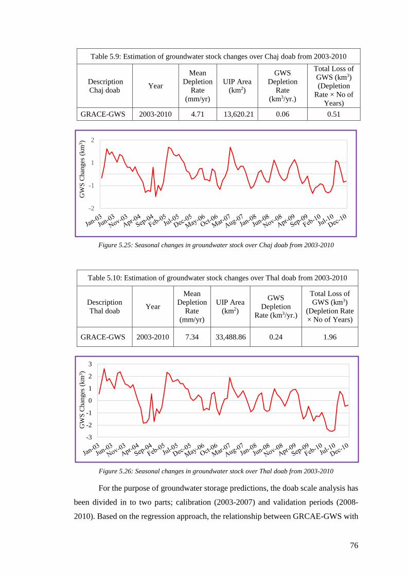
76
Table 5.9: Estimation of groundwater stock changes over Chaj doab from 2003-2010
Description
Chaj doab Year
Mean
Depletion
Rate
(mm/yr)
UIP Area
(km2)
GWS
Depletion
Rate
(km3/yr.)
Total Loss of
GWS (km3)
(Depletion
Rate × No of
Years)
GRACE-GWS 2003-2010 4.71 13,620.21 0.06 0.51
Figure 5.25: Seasonal changes in groundwater stock over Chaj doab from 2003-2010
Table 5.10: Estimation of groundwater stock changes over Thal doab from 2003-2010
Description
Thal doab Year
Mean
Depletion
Rate
(mm/yr)
UIP Area
(km2)
GWS
Depletion
Rate (km3/yr.)
Total Loss of
GWS (km3)
(Depletion Rate
× No of Years)
GRACE-GWS 2003-2010 7.34 33,488.86 0.24 1.96
Figure 5.26: Seasonal changes in groundwater stock over Thal doab from 2003-2010
For the purpose of groundwater storage predictions, the doab scale analysis has
been divided in to two parts; calibration (2003-2007) and validation periods (2008-
2010). Based on the regression approach, the relationship between GRCAE-GWS with
-3
-2
-1
0
1
2
3
GW
S C
han
ges
(km
3)
-2
-1
1
2
GW
S C
han
ges
(km
3)
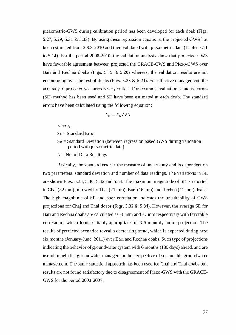
77
piezometric-GWS during calibration period has been developed for each doab (Figs.
5.27, 5.29, 5.31 & 5.33). By using these regression equations, the projected GWS has
been estimated from 2008-2010 and then validated with piezometric data (Tables 5.11
to 5.14). For the period 2008-2010, the validation analysis show that projected GWS
have favorable agreement between projected the GRACE-GWS and Piezo-GWS over
Bari and Rechna doabs (Figs. 5.19 & 5.20) whereas; the validation results are not
encouraging over the rest of doabs (Figs. 5.23 & 5.24). For effective management, the
accuracy of projected scenarios is very critical. For accuracy evaluation, standard errors
(SE) method has been used and SE have been estimated at each doab. The standard
errors have been calculated using the following equation;
𝑆𝐸 = 𝑆𝐷 √𝑁⁄
where;
SE = Standard Error
SD = Standard Deviation (between regression based GWS during validation
period with piezometric data)
N = No. of Data Readings
Basically, the standard error is the measure of uncertainty and is dependent on
two parameters; standard deviation and number of data readings. The variations in SE
are shown Figs. 5.28, 5.30, 5.32 and 5.34. The maximum magnitude of SE is reported
in Chaj (32 mm) followed by Thal (21 mm), Bari (16 mm) and Rechna (11 mm) doabs.
The high magnitude of SE and poor correlation indicates the unsuitability of GWS
projections for Chaj and Thal doabs (Figs. 5.32 & 5.34). However, the average SE for
Bari and Rechna doabs are calculated as ±8 mm and ±7 mm respectively with favorable
correlation, which found suitably appropriate for 3-6 monthly future projection. The
results of predicted scenarios reveal a decreasing trend, which is expected during next
six months (January-June, 2011) over Bari and Rechna doabs. Such type of projections
indicating the behavior of groundwater system with 6 months (180 days) ahead, and are
useful to help the groundwater managers in the perspective of sustainable groundwater
management. The same statistical approach has been used for Chaj and Thal doabs but,
results are not found satisfactory due to disagreement of Piezo-GWS with the GRACE-
GWS for the period 2003-2007.
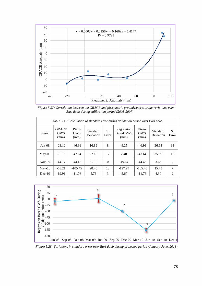
78
Table 5.11: Calculation of standard error during validation period over Bari doab
Period
GRACE
GWS
(mm)
Piezo
GWS
(mm)
Standard
Deviation
S.
Error
Regression
Based GWS
(mm)
Piezo
GWS
(mm)
Standard
Deviation
S.
Error
Jun-08 -23.12 -46.91 16.82 8 -9.25 -46.91 26.62 12
May-09 -9.19 -47.64 27.18 12 2.40 -47.64 35.39 16
Nov-09 -44.17 -44.45 0.19 0 -49.64 -44.45 3.66 2
May-10 -65.21 -105.45 28.45 13 -127.29 -105.45 15.43 7
Dec-10 -19.91 -11.76 5.76 3 -5.67 -11.76 4.30 2
Figure 5.28: Variations in standard error over Bari doab during projected period (January-June, 2011)
12
16
2
7
2
-150
-125
-100
-75
-50
-25
0
25
50
Jun-08 Sep-08 Dec-08 Mar-09 Jun-09 Sep-09 Dec-09 Mar-10 Jun-10 Sep-10 Dec-10
Reg
ress
ion B
ased
GW
S D
uri
ng
Val
idat
ion P
erio
d (
mm
)
y = 0.0002x3 - 0.0156x2 + 0.1669x + 5.4147
R² = 0.9721
-20
-10
0
10
20
30
40
50
60
70
80
-40 -20 0 20 40 60 80 100
GR
AC
E A
no
mal
y (
mm
)
Piezometric Anomaly (mm)
Figure 5.27: Correlation between the GRACE and piezometric groundwater storage variations over
Bari doab during calibration period (2003-2007)
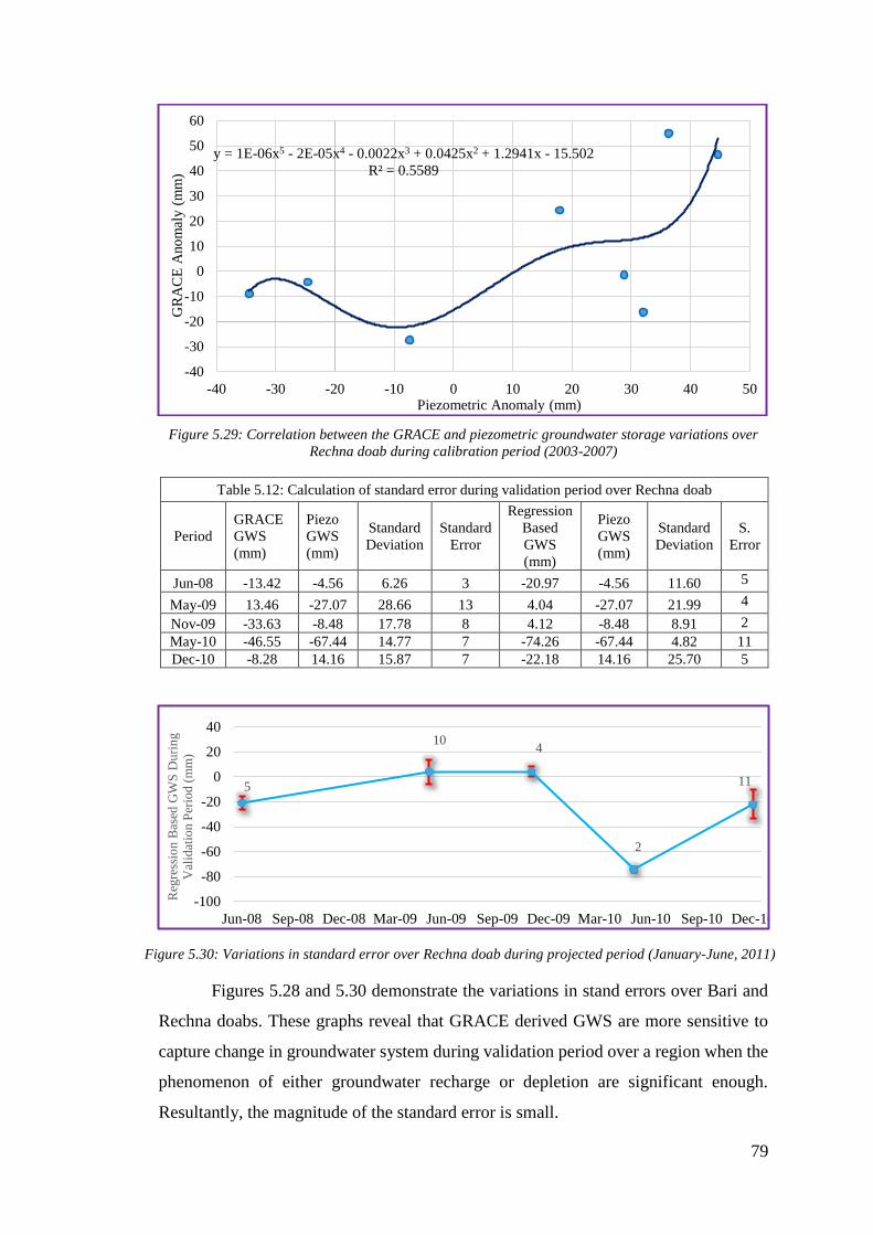
79
Figure 5.29: Correlation between the GRACE and piezometric groundwater storage variations over
Rechna doab during calibration period (2003-2007)
Table 5.12: Calculation of standard error during validation period over Rechna doab
Period
GRACE
GWS
(mm)
Piezo
GWS
(mm)
Standard
Deviation
Standard
Error
Regression
Based
GWS
(mm)
Piezo
GWS
(mm)
Standard
Deviation
S.
Error
Jun-08 -13.42 -4.56 6.26 3 -20.97 -4.56 11.60 5
May-09 13.46 -27.07 28.66 13 4.04 -27.07 21.99 4
Nov-09 -33.63 -8.48 17.78 8 4.12 -8.48 8.91 2
May-10 -46.55 -67.44 14.77 7 -74.26 -67.44 4.82 11
Dec-10 -8.28 14.16 15.87 7 -22.18 14.16 25.70 5
Figures 5.28 and 5.30 demonstrate the variations in stand errors over Bari and
Rechna doabs. These graphs reveal that GRACE derived GWS are more sensitive to
capture change in groundwater system during validation period over a region when the
phenomenon of either groundwater recharge or depletion are significant enough.
Resultantly, the magnitude of the standard error is small.
y = 1E-06x5 - 2E-05x4 - 0.0022x3 + 0.0425x2 + 1.2941x - 15.502
R² = 0.5589
-40
-30
-20
-10
0
10
20
30
40
50
60
-40 -30 -20 -10 0 10 20 30 40 50
GR
AC
E A
no
mal
y (
mm
)
Piezometric Anomaly (mm)
5
104
2
11
-100
-80
-60
-40
-20
0
20
40
Jun-08 Sep-08 Dec-08 Mar-09 Jun-09 Sep-09 Dec-09 Mar-10 Jun-10 Sep-10 Dec-10
Reg
ress
ion
Bas
ed G
WS
Du
rin
g
Val
idat
ion
Per
iod
(m
m)
Figure 5.30: Variations in standard error over Rechna doab during projected period (January-June, 2011)
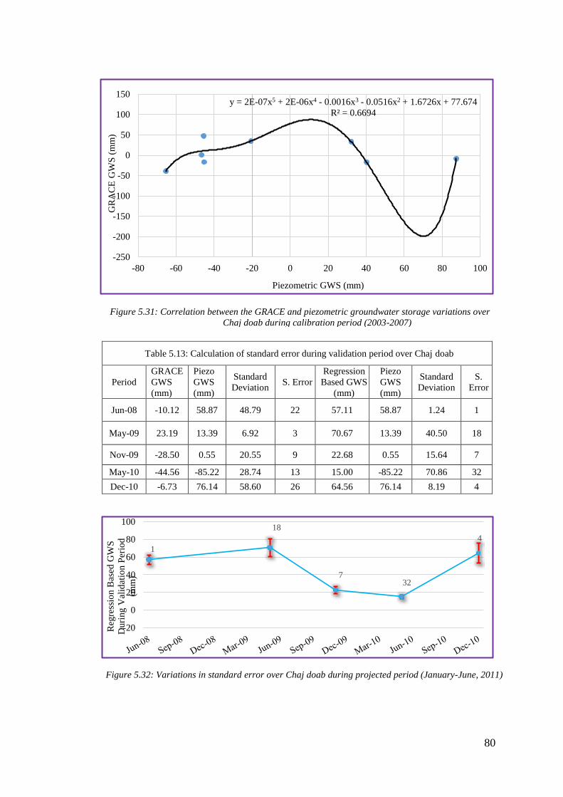
80
Table 5.13: Calculation of standard error during validation period over Chaj doab
Period
GRACE
GWS
(mm)
Piezo
GWS
(mm)
Standard
Deviation S. Error
Regression
Based GWS
(mm)
Piezo
GWS
(mm)
Standard
Deviation
S.
Error
Jun-08 -10.12 58.87 48.79 22 57.11 58.87 1.24 1
May-09 23.19 13.39 6.92 3 70.67 13.39 40.50 18
Nov-09 -28.50 0.55 20.55 9 22.68 0.55 15.64 7
May-10 -44.56 -85.22 28.74 13 15.00 -85.22 70.86 32
Dec-10 -6.73 76.14 58.60 26 64.56 76.14 8.19 4
y = 2E-07x5 + 2E-06x4 - 0.0016x3 - 0.0516x2 + 1.6726x + 77.674
R² = 0.6694
-250
-200
-150
-100
-50
0
50
100
150
-80 -60 -40 -20 0 20 40 60 80 100
GR
AC
E G
WS
(m
m)
Piezometric GWS (mm)
1
18
732
4
-20
0
20
40
60
80
100
Reg
ress
ion B
ased
GW
S
Duri
ng V
alid
atio
n P
erio
d
(mm
)
Figure 5.32: Variations in standard error over Chaj doab during projected period (January-June, 2011)
Figure 5.31: Correlation between the GRACE and piezometric groundwater storage variations over
Chaj doab during calibration period (2003-2007)
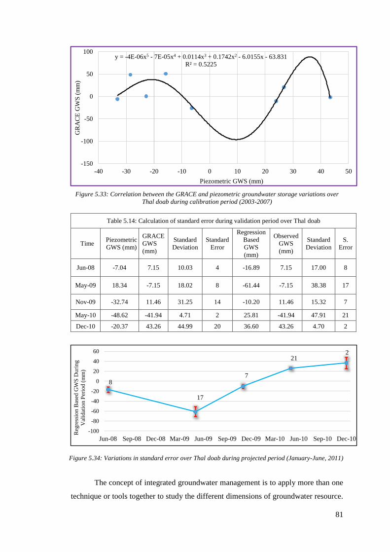
81
Figure 5.33: Correlation between the GRACE and piezometric groundwater storage variations over
Thal doab during calibration period (2003-2007)
Table 5.14: Calculation of standard error during validation period over Thal doab
Time Piezometric
GWS (mm)
GRACE
GWS
(mm)
Standard
Deviation
Standard
Error
Regression
Based
GWS
(mm)
Observed
GWS
(mm)
Standard
Deviation
S.
Error
Jun-08 -7.04 7.15 10.03 4 -16.89 7.15 17.00 8
May-09 18.34 -7.15 18.02 8 -61.44 -7.15 38.38 17
Nov-09 -32.74 11.46 31.25 14 -10.20 11.46 15.32 7
May-10 -48.62 -41.94 4.71 2 25.81 -41.94 47.91 21
Dec-10 -20.37 43.26 44.99 20 36.60 43.26 4.70 2
Figure 5.34: Variations in standard error over Thal doab during projected period (January-June, 2011)
The concept of integrated groundwater management is to apply more than one
technique or tools together to study the different dimensions of groundwater resource.
y = -4E-06x5 - 7E-05x4 + 0.0114x3 + 0.1742x2 - 6.0155x - 63.831
R² = 0.5225
-150
-100
-50
0
50
100
-40 -30 -20 -10 0 10 20 30 40 50
GR
AC
E G
WS
(m
m)
Piezometric GWS (mm)
8
17
7
212
-100
-80
-60
-40
-20
0
20
40
60
Jun-08 Sep-08 Dec-08 Mar-09 Jun-09 Sep-09 Dec-09 Mar-10 Jun-10 Sep-10 Dec-10
Reg
ress
ion
Bas
ed G
WS
Du
rin
g
Val
idat
ion
Per
iod
(m
m)
82
The spatio-temporal analysis of groundwater system behavior has necessitated applying
an integrated approach for both groundwater monitoring and management perspective.
The earlier discussion has elaborated in detail about the opportunities and challenges
associated with different monitoring tools (modeling, in-situ measurements and remote
sensing) in practice for groundwater management. The analysis of the GRACE
groundwater storage variations, piezometric water table fluctuations and VMOD
groundwater system behavior, indicate that Bari doab and parts of Rechna, Chaj and
Thal doabs are experiencing groundwater depletion. More specifically, the groundwater
sustainability is at risk in Bari doab due to unbalance between recharge and abstraction.
Due to low rainfall and low flows in eastern Rivers, the over abstraction disturbances
the groundwater balance. The Bari doab (Fig. 5.14) in general and especially, the areas
of Khanewal, Lodhran and Multan (Fig. 5.3) need immediate attention with appropriate
mitigation strategies where foremost required suggested measure is controlled
abstraction with continuous monitoring.
In this situation, GARCE is found useful for continuous monthly tracking of
groundwater storage whereas, the piezometers network may be helpful at seasonal to
annual scale. There is also need for detailed modeling to devise region specific and
appropriate management strategies. The modeling approach is essentially required at
annual scale for better understanding of surface water and groundwater interactions by
incorporating the climatic implications. Secondly, it is also important to adopt water
conservation approaches and especially, education of farming community could play a
major role by changing their minds to conserve water. Currently, the most of useable
water is wasted at farm scale due to traditional flood irrigation practice through which
unnecessarily farmers are irrigation many times than the actual requirements of those
crops. The rainwater harvesting is another area, which needs to be harvested for
recharge enhancement. In Rechna doab, the situation is relatively better than Bari doab
where enough recharge is available from multiple sources (Rivers, irrigation system,
rainfall). The analysis show that the floods also play their role in recharging the Rechna
doab. However, the tube well density in Rechna doab is also higher (0.104 tube wells
per hectare) where huge groundwater abstraction is happing through 0.33 million tube
wells (Bureau of Statistics 2012). Keeping in view this over-exploitation, the
groundwater depletion is expected to become more critical in the lower Rechna doab in
future (Khan et al. 2008). The controlled abstraction is suggested with the adoption of
83
water conservation techniques for sustainable groundwater management. The efforts
are also required to increase the groundwater recharge by artificial techniques.
There is continuous need of groundwater monitoring and the GRACE is
recommended for monthly monitoring in an integrated way along with VMOD and
piezometric datasets. Actually, all these three tools will complement each other for
accuracy improvement. Having small area and sufficient recharge from adjacent rivers,
Chaj is comparatively safer except the lower parts where considerable depletion is
observed. Similarly, Thal doab is also safe except in few areas of upper Thal where the
water table depletion has been observed. Therefore, a careful groundwater monitoring
is needed along with water conservation practice. The urbanization challenge may
impact the recharge so, the protection of recharge areas may be considered. Due to a
number of challenges (small area, coarse resolution, sporadic piezometric datasets,
intermixed phenomenon and low accuracy), the GRACE is not suitable to apply for
monitoring purposes in Chaj and Thal doabs. The term intermixed phenomenon is
referred to a place where both groundwater recharge and depletion happen
simultaneously.
5.5 GRACE – A Spatial Decision Support Tool
To devise appropriate management strategies, the role of decision support
system is critically important to facilitate the managers and policy makers in
understanding or assessing the severity of the complex issues and assist them in
developing the appropriate mitigation strategies. Being hidden resource, the spatial
variability in groundwater dynamics is more complex and needs integration of various
techniques and tools. In this perspective, the GRACE has proven its practical ability
over Bari and Rechna doabs for adoption as decision support tool. The demonstration
of the GRACE for 3-6 monthly projections (Fig. 5.20 & 5.21) of groundwater storage
anomalies is a good opportunity for its practical adoption and further development as
decision support system. Therefore, its integration with GIS is a good example for
further development of a decision support system. Such application is envisioned, not
only to serve as information management system but, maximizing its ability to perform
various operations such as query, calculation, scenario building, etc. The coupling of
supplementary information from other remote sensing sensors/products and ground
measurements potentially help improve the system efficiency through overlaying
capabilities.
84
5.6 Tracking Groundwater from Space
5.6.1 Opportunities
The global coverage with free and frequent data availability are the key feature
of remote sensing technology such as the GRACE. The GRACE has enabled basin-
wide hydrological studies and as well as evaluation of global aquifers. In past, it was a
big challenge due to the scarcity of observed or measured data. The second major
feature is its ability to measure the complete water cycle, which otherwise was very
difficult. The rest of the satellite sensors are parameter specific missions like, GPM
(Global Precipitation Measurement Mission), SMAP (Soil Moisture Active Passive,
TRMM (Tropical Rainfall Measurement Mission), altimetry (water levels
measurement), etc. The GRACE has empowered the scientific community with analysis
liberty. The hydrologist have now more flexibility and liberty either they want to work
on any specific component/parameter of water cycle or basin scale budgeting by
analyzing the water cycle as a whole. Thirdly, the trans-boundary applications is
another added advantage. The application of the GRACE in combination with satellite
altimetry and precipitation products, potentially a good opportunity for hydrologist to
study trans-boundary issues especially in developing countries. The data sharing is a
big issue in developing countries. The upstream countries do not share accurate and
timely information with countries at downstream who are at the verge of vulnerability
to extreme and devastating climatic implications. The fourth major advantage is the
integration of satellite data with hydrological modeling. Both the satellite and
hydrological models are complimented from each other. The satellite data is used as
input for hydrological simulations as well as calibration of modeling outputs in data
deficit regions or ungauged basins. Whereas, the calibrated modeling simulations are
used for the calibration of satellite driven applications.
5.6.2 Challenges
Besides opportunities, the challenges are also there, which limits the societal
benefits of the GRACE as an effective tool for groundwater resource management in
developing countries in general and Indus Basin specifically. The foremost of them is
its inherent limitation of coarse spatial resolution, which not only effects the accuracy
of results but also its applicability at small spatial scales (Rodell et al. 2009). There is
always a tradeoff between accuracy and spatial coverage. The GRACE data latency is
another challenge, which hampers its real time applicability. The launching of the
85
GRACE-FO mission in May, 2018 is anticipated to manage this issue having higher
spatial resolution. The GRACE data becomes publicly available after 1-2 months from
the time of its data collection. The data processing takes time due to system
complexities through which, it collects the gravity anomalies. The data processing
centers (CSR, GFZ, and JPL) release the GRACE data in the form of spherical harmonic
coefficients after initial processing of gravity anomalies. It is a critical concern from
the user end (groundwater managers, policy makers) because; the instant information
is required for timely implementation. The GRACE mission team has to overcome this
issue for its wide applicability. However, the GRACE driven time series information is
good to get the historical picture of groundwater system.
The second major concern is the non-availability of the GRACE data processing
tools in public domain and involve technical complexities. As the gravimetry is a
complex science, the derivation of total water storage information from gravity field
involves a lot of processing. For this purpose, relevant professionals and expertise are
required to be developed for organizational scale adoptability. The role of NASA
applied science team is important for the promotion of the GRACE technology through
upscaling of capacity building programs. The facilitation in terms of capacity building
efforts and provision of relevant tools in public domain potentially help to accelerate
the GRACE integrated applications for societal benefits.
86
CHAPTER 6
Conclusion and Recommendations
6.1 Conclusions
Generally, the GRACE derived spatial variations in groundwater storage helps
to understand the seasonal to annual changes, assess the spatial patterns of groundwater
use, identify the critically under-stress areas with over-exploitation areas and quantify
the groundwater recharge from various sources along with supplementary information.
More specifically, the analysis and detailed deliberations derive the following
conclusions;
1. The analysis of average trend of total water storage and subsequent changes in
groundwater storage anomalies suggest that the variations over UIP are more
rapid as compared to other parts of Indus Basin in Pakistan. The TWS has
decreased about two times more over UIP (19.5 mm per year) than the whole
Indus Basin (10.1 mm per year) from 2003 to 2010. It reveals that UIP dominates
the hydrology of Indus Basin due to extensive groundwater abstraction for
anthropogenic purposes.
2. The comparison of the VIC with GLDAS-1 reveals that the impact of the selection
of land surface model becomes insignificant while comparing the trends of
groundwater storage anomalies however, a modest quantitative difference has
appear in the results of two models. The results of the VIC simulations indicated
that the selection of appropriate model and basin specific modeling is much useful
rather than using global modeling outputs.
3. The GRACE has found successful (correlation with observed data = 0.58) in
capturing both, the trend and magnitude of groundwater fluctuations averagely at
seasonal to annual scale over UIP. The spatial analysis of annual change detection
has revealed that the groundwater storage has been changed more rapidly over
Bari and Rechna doabs in comparison with Chaj and Thal over the period 2003-
2010.
4. While analysis the local variations at individual doabs, the results suggest that
numerical down scaling (at 0.1˚ × 0.1˚) approach has performed better and
effective as compared to actual GWS at 1˚ × 1˚ grid scaling. Out of four doabs,
the GRACE found more capable in Bari and Rechna doabs and has successfully
87
captured seasonal groundwater storage trends in good agreement (correlation =
0.93 for Bari and 0.65 for Rechna) with piezometric data. The GRACE has
reported groundwater depletion of about 0.38 and 0.21 km3 per year in Bari and
Rechna doabs respectively. Whereas, a disagreement between the GRACE and
piezometric data is reported in Chaj and Thal doabs may be due to sporadic nature
of piezometric records with low frequency during the study period. However, the
GRACE based depletion trends are quite verified by VMOD for both Chaj and
Thal doabs.
5. The groundwater aquifer in Bari doab area is under severe stress whereas the
condition in Rechna doab is moderate whereas, Chaj and Thal doabs are
comparatively safer. The persistent and significant groundwater depletion is
prevalent in Bari and Rechna doabs whereas, sub-doab scale intermixed trends of
groundwater depletion and recharge are more visible in Chaj and Thal doabs.
6. Furthermore, the groundwater depletion is taking place in the areas of Lower Bari
doab (Multan, Lodhran, Khanewal including Lahore), some parts of Rechna
(Toba Tek Singh and parts of the Jhang districts) and Chaj (Sargodha district).
The Chaj and Thal doabs are comparatively safer. In Lower Thal doab, the
GRACE has measured groundwater depletion, which is contradictory with
observational measurements and ground conditions (small strip with enough
recharge from bounding rivers, which are at a short distance). It is due to the
limitations of the GRACE in the form of its legacy of being coarse spatial
resolution satellite.
7. The integrated approach comprising of satellite, groundwater modeling and
groundwater measurement network is found effective at doab to Indus Basin
scales, for appropriate monitoring and management of groundwater resource.
8. While investigation, it is estimated that UIP has lost a stock of about 11.84 km3
fresh groundwater storage in just 8 years of time (2003-2010) through extensive
groundwater abstraction. The projected scenario (2011-2014) indicated further
loss of fresh groundwater storage due to increasing dependence on groundwater.
It is found that the role of flooding events in the replenishment of groundwater is
very observant in UIP due to its favorable lithology. In Pakistan, the flooding
events of 2010 and 2014 has facilitated in reducing average depletion rates from
88
13.5 (2003-2010) to 5.3 mm (2011-2014) per year over UIP. Thereof, it is
expected that the groundwater storage of about 3.59 km3 will be added as recharge
to the groundwater system during the period 2011-2014.
9. The evaluation of statistical approach for future projection resulted an average
standard error (SE) of 8 mm and 7 mm in Bari and Rechna doabs respectively
with favorable correlation and found suitably appropriate for 3-6 monthly future
projection. However, this technique is not found appropriate for Chaj and Bari
doabs due to disagreement with Piezo-GWS over the calibration period.
10. As a decision support tool, the GRACE has demonstrated well for 3-6 monthly
projections, which would hold true for 2-3 months over UIP. It is revealed that
the applicability of decision support tool is more valid over Bari and Rechna
doabs.
6.2 Recommendations
Based on the results and discussion, the summary of the recommendation and
future directions are listed as below;
1. Keeping in view the inherent coarse resolution, the accuracy of the GRACE
derived GWS is very much depended on the accurate simulations of soil moisture
and surface water fluxes through hydrological modeling. To bridge the in-situ data
paucity, the evaluation of the potential of satellite-based soil moisture products
such as SMAP is considered important for further utilization in the derivation of
groundwater storage anomalies.
2. The synthesis of results suggests that the identified critical areas of Lower Bari
(Multan, Khanewal, Lodhran including Lahore) and few regions of Rechna (Toba
Tek Singh, Chiniot, Jhang, Narowal) need immediate attention. The controlled
abstraction, continuous monitoring of groundwater levels, water conservation and
artificial groundwater recharge (both surface and rainwater) practices are
recommended from implementation in these areas. In these areas, the detailed
(local scale) groundwater modeling is importantly required and would be helpful
for devising more appropriate groundwater management strategies.
3. For better calibration of satellite remote sensing (GRACE) and hydrological
models, the ground observation network (piezometers) is required to be further
89
strengthen through the installation of automatic groundwater loggers. It would
help to automatically record water level datasets with high temporal frequency
(10 daily or monthly), which would be useful for accurate calibration of satellite
products and modeling simulation.
4. The projection of groundwater storage could be improved during the regime
transition phase from non-Monsoon to Monsoon seasons by supplementing the
information of groundwater pumping and rainfall patterns.
5. There is also need to enhance the spatial resolution of the GRACE satellite for
better accuracy through integration with other appropriate satellite datasets. For
this purpose, Synthetic Aperture Radar and satellite altimetry could be the
potential products for spatial downscaling of the GRACE signal.
6. The study of relationship between climatic variables with groundwater storage
changes is important to analyze the future scenarios in the perspective of climatic
impacts on water resources.
90
References
Ahmad, N. (1993). Water resources of Pakistan. Publisher Shahzad Nazir, Gulberg, Lahore,
Pakistan
Ahmad, W., Fatima, A., Awan, U.K., & Anwar, A. (2014). Analysis of long term
meteorological trends in the middle and lower Indus Basin of Pakistan—A non-
parametric statistical approach. Global and Planetary Change, 122, 282-291
Alam, N., & Olsthoorn, T.N. (2014). Punjab scavenger wells for sustainable additional
groundwater irrigation. Agricultural Water Management, 138, 55-67
Ashraf, A., & Ahmad, Z. (2008). Regional groundwater flow modelling of Upper Chaj Doab
of Indus Basin, Pakistan using finite element model (Feflow) and geoinformatics.
Geophysical Journal International, 173, 17-24
Ashraf, M., Zeeshan, A.B., & Zakaullah (2012). Diagnostic analysis and fine tuning of
skimming well design and operational strategies for sustainable groundwater
management - Indus basin of Pakistan. Irrigation and Drainage, 61, 270-282
Awan, U.K., & Ismaeel, A. (2014). A new technique to map groundwater recharge in irrigated
areas using a SWAT model under changing climate. Journal of Hydrology, 519, 1368-
1382
Bandaragoda, D.J. (1995). Warabandi in Pakistan's canal irrigation systems: Widening gap
between theory and practice. IWMI
Basharat, M., & Tariq, A.-u.-R. (2015). Groundwater modelling for need assessment of
command scale conjunctive water use for addressing the exacerbating irrigation cost
inequities in LBDC irrigation system, Punjab, Pakistan. Sustainable Water Resources
Management, 1, 41-55
Basharat, M., & Tariq, A.U.R. (2013). Long‐term groundwater quality and saline intrusion
assessment in an irrigated environment: A case study of the aquifer under the lbdc
irrigation system. Irrigation and Drainage, 62, 510-523
Basharat, M., Umair Ali, S., & Azhar, A.H. (2014). Spatial variation in irrigation demand and
supply across canal commands in Punjab: a real integrated water resources
management challenge. Water Policy, 16, 397-421
Bennett, G.D., Sheikh, I.A., & Alr, S. (1967). Analysis of aquifer tests in the Punjab region of
West Pakistan. In, Water Supply Paper
Bhutta, M.N., & Sufi, A. (2004). A Perspective scenario of water for irrigated agriculture in
Pakistan. In, Proceedings of Pakistan Engineering Congress
Bonsor, H., MacDonald, A., Ahmed, K., Burgess, W., Basharat, M., Calow, R., Dixit, A.,
Foster, S., Gopal, K., & Lapworth, D. (2017). Hydrogeological typologies of the Indo-
Gangetic basin alluvial aquifer, South AsiaTypologies hydrogéologiques de l’aquifère
alluvial du bassin de l’Indus et du Gange, Asie du SudTipologías hidrogeológicas del
acuífero aluvial de la cuenca Indo-Gangética, Asia Meridional Tipologias
hidrogeológicas do aquífero aluvial da bacia Indo-Gangética, Sul da Ásia.
Hydrogeology Journal, 25, 1377-1406
Brunner, P., Hendricks Franssen, H.-J., Kgotlhang, L., Bauer-Gottwein, P., & Kinzelbach, W.
(2007). How can remote sensing contribute in groundwater modeling? Hydrogeology
Journal, 15, 5-18
Bureau of Statistics (2012). Punjab Development Statistics. In. Lahore. Pakistan: Government
of the Punjab
Bhanja, Soumendra N., Abhijit Mukherjee, Dipankar Saha, Isabella Velicogna, and James S.
Famiglietti. (2016a). “Validation of GRACE Based Groundwater Storage Anomaly
91
Using In-Situ Groundwater Level Measurements in India.” Journal of Hydrology, 543
(December): 729–38
Bhanja, Soumendra N., Matthew Rodell, Bailing Li, Dipankar Saha, and Abhijit Mukherjee.
(2016b). “Spatio-Temporal Variability of Groundwater Storage in India.” Journal of
Hydrology, 544 (January): 428–37.
Bhanja, S.N., Mukherjee, A., Rodell, M. et al. (2017). Groundwater rejuvenation in parts of
India influenced by water-policy change implementation. Scientific Reports 7,
DOI:10.1038/s41598-017-07058-2
Chandio, A., Lee, T., & Mirjat, M. (2012). The extent of waterlogging in the lower Indus Basin
(Pakistan)–A modeling study of groundwater levels. Journal of Hydrology, 426, 103-
111
Chao, B.F., & Gross, R.S. (1987). Changes in the Earth's rotation and low‐degree gravitational
field induced by earthquakes. Geophysical Journal of the Royal Astronomical Society,
91, 569-596
Cheema, M.J.M., Immerzeel, W.W., & Bastiaanssen, W.G.M. (2014). Spatial Quantification
of Groundwater Abstraction in the Irrigated Indus Basin. Groundwater, 52, 25-36
Chen, J., Jönsson, P., Tamura, M., Gu, Z., Matsushita, B., & & Eklundh, L. (2004). A simple
method for reconstructing a high-quality NDVI time-series data set based on the
Savitzky–Golay filter. Remote Sensing of Environment, 91, 332-344
Döll, P., Hoffmann-Dobrev, H., Portmann, F.T., Siebert, S., Eicker, A., Rodell, M., Strassberg,
G., & Scanlon, B.R. (2012). Impact of water withdrawals from groundwater and
surface water on continental water storage variations. Journal of Geodynamics, 59-60,
143-156
Duan, X.J., Guo, J.Y., Shum, C.K., & van der Wal, W. (2009). On the postprocessing removal
of correlated errors in GRACE temporal gravity field solutions. Journal of Geodesy,
83, 1095
Falkenmark, M., Berntell, A., Jägerskog, A., Lundqvist, J., Matz, M., & Tropp, H. (2007). On
the Verge of a New Water Scarcity: A Call for Good Governance and Human
Ingenuity. In
Famiglietti, J., Lo, M., Ho, S., Bethune, J., Anderson, K., Syed, T., Swenson, S., De Linage,
C., & Rodell, M. (2011). Satellites measure recent rates of groundwater depletion in
California's Central Valley. Geophysical Research Letters, 38
Federal Flood Commission (2017). Annual Flood Rport 2017. In. Islamabad, Pakistan: Federal
Flood Commission, Ministry of Water Resources
Feng, W., Zhong, M., Lemoine, J.M., Biancale, R., Hsu, H.T., & Xia, J. (2013). Evaluation of
groundwater depletion in North China using the Gravity Recovery and Climate
Experiment (GRACE) data and ground‐based measurements. Water Resources
Research, 49, 2110-2118
Foster, S., & MacDonald, A. (2014). The ‘water security’dialogue: why it needs to be better
informed about groundwater. Hydrogeology Journal, 22, 1489-1492
Gleeson, T., Wada, Y., Bierkens, M.F., & van Beek, L.P. (2012). Water balance of global
aquifers revealed by groundwater footprint. Nature, 488, 197
Greenman, D.W., Swarzenski, W.V., & Bennett, G.D. (1967). Ground-water hydrology of the
Punjab, West Pakistan, with emphasis on problems caused by canal irrigation. US
Government Printing Office
Guo, J., Duan, X., & Shum, C. (2010). Non-isotropic Gaussian smoothing and leakage
reduction for determining mass changes over land and ocean using GRACE data.
Geophysical Journal International, 181, 290-302
Hanif, M., Khan, A.H., & Adnan, S. (2013). Latitudinal precipitation characteristics and trends
in Pakistan. Journal of Hydrology, 492, 266-272
92
Jin, S., & Feng, G. (2013). Large-scale variations of global groundwater from satellite
gravimetry and hydrological models, 2002–2012. Global and Planetary Change, 106,
20-30
Khan, A.D., Iqbal, N., Ashraf, M., & Ashfaq, A.S. (2016a). Groundwater investigations and
mapping in the Upper Indus Plain. In (p. 72). Islamabad, Pakistan: Pakistan Council
of Research in Water Resources
Khan, H.F., Yang, Y.E., Ringler, C., Wi, S., Cheema, M., & Basharat, M. (2016b). Guiding
Groundwater Policy in the Indus Basin of Pakistan Using a Physically Based
Groundwater Model. Journal of Water Resources Planning and Management, 143,
05016014
Khan, S., Rana, T., Gabriel, H., & Ullah, M.K. (2008). Hydrogeologic assessment of escalating
groundwater exploitation in the Indus Basin, Pakistan. Hydrogeology Journal, 16,
1635-1654
Konikow, L.F. (2011). Contribution of global groundwater depletion since 1900 to sea‐level
rise. Geophysical Research Letters, 38
Kummerow, C., Barnes, W., Kozu, T., Shiue, J., & Simpson, J. (1998). The tropical rainfall
measuring mission (TRMM) sensor package. Journal of atmospheric and oceanic
technology, 15, 809-817
Kusche, J. (2007). Approximate decorrelation and non-isotropic smoothing of time-variable
GRACE-type gravity field models. Journal of Geodesy, 81, 733-749
Latif, M., & Syed, F. (2016). Determination of summer monsoon onset and its related large-
scale circulation characteristics over Pakistan. Theoretical and applied climatology,
125, 509-520
Lee, H., Beighley, R.E., Alsdorf, D., Jung, H.C., Shum, C.K., Duan, J., Guo, J., Yamazaki, D.,
& Andreadis, K. (2011). Characterization of terrestrial water dynamics in the Congo
Basin using GRACE and satellite radar altimetry. Remote Sensing of Environment,
115, 3530-3538
Liang, X., Lettenmaier, D.P., Wood, E.F., & Burges, S.J. (1994). A simple hydrologically
based model of land surface water and energy fluxes for general circulation models.
Journal of Geophysical Research: Atmospheres, 99, 14415-14428
Long, D., Longuevergne, L., & Scanlon, B.R. (2014). Uncertainty in evapotranspiration from
land surface modeling, remote sensing, and GRACE satellites. Water Resources
Research, 50, 1131-1151
Longuevergne, L., Scanlon, B.R., & Wilson, C.R. (2010). GRACE Hydrological estimates for
small basins: Evaluating processing approaches on the High Plains Aquifer, USA.
Water Resources Research, 46
Moore, S., & Fisher, J.B. (2012). Challenges and opportunities in GRACE-based groundwater
storage assessment and management: an example from Yemen. Water resources
management, 26, 1425-1453
Moriasi, D.N., Arnold, J.G., Van Liew, M.W., Bingner, R.L., Harmel, R.D., & Veith, T.L.
(2007). Model evaluation guidelines for systematic quantification of accuracy in
watershed simulations. Transactions of the ASABE, 50, 885-900
Mukherjee, Abhijit, Dipankar Saha, Charles F. Harvey, Richard G. Taylor, Kazi Matin Ahmed,
and Soumendra N. Bhanja. (2015). “Groundwater Systems of the Indian Sub-
Continent.” Journal of Hydrology: Regional Studies 4: 1–14
Mundorff, M.J., Carrigan Jr, P., Steele, T., & Randall, A. (1976). Hydrologic evaluation of
salinity control and reclamation projects in the Indus Plain, Pakistan--A summary. In:
US Govt. Print. Off.
93
Qureshi, A.S., McCornick, P.G., Qadir, M., & Aslam, Z. (2008). Managing salinity and
waterlogging in the Indus Basin of Pakistan. Agricultural Water Management, 95, 1-
10
Qureshi, A.S., McCornick, P.G., Sarwar, A., & Sharma, B.R. (2010). Challenges and prospects
of sustainable groundwater management in the Indus Basin, Pakistan. Water resources
management, 24, 1551-1569
Qureshi, A.S., Shah, T., & Akhtar, M. (2003). The groundwater economy of Pakistan. IWMI
Rodell, M., Chen, J., Kato, H., Famiglietti, J.S., Nigro, J., & Wilson, C.R. (2007). Estimating
groundwater storage changes in the Mississippi River basin (USA) using GRACE.
Hydrogeology Journal, 15, 159-166
Rodell, M., Velicogna, I., & Famiglietti, J.S. (2009). Satellite-based estimates of groundwater
depletion in India. Nature, 460, 999
Saeed, M., & Ashraf, M. (2005). Feasible design and operational guidelines for skimming wells
in the Indus basin, Pakistan. Agricultural Water Management, 74, 165-188
Scanlon, B., Gates, J., Reedy, R., Jackson, W., & Bordovsky, J. (2010). Effects of irrigated
agroecosystems: 2. Quality of soil water and groundwater in the southern High Plains,
Texas. Water Resources Research, 46
Scanlon, B.R., Longuevergne, L., & Long, D. (2012). Ground referencing GRACE satellite
estimates of groundwater storage changes in the California Central Valley, USA.
Water Resources Research, 48
Shum, C.K., Guo, J.-Y., Hossain, F., Duan, J., Alsdorf, D., Duan, X., Kuo, C.Y., Lee, H.,
Schmidt, M., & Wang, L. (2011). Inter-annual Water Storage Changes in Asia from
GRACE Data.
Siddique-E-Akbor, A., Hossain, F., Sikder, S., Shum, C., Tseng, S., Yi, Y., Turk, F., & Limaye,
A. (2014). Satellite precipitation data–driven hydrological modeling for water
resources management in the Ganges, Brahmaputra, and Meghna Basins. Earth
Interactions, 18, 1-25
Siebert, S., Burke, J., Faures, J.-M., Frenken, K., Hoogeveen, J., Döll, P., & Portmann, F.T.
(2010). Groundwater use for irrigation–a global inventory. Hydrology and Earth
System Sciences, 14, 1863-1880
Singh, A. (2014). Groundwater resources management through the applications of simulation
modeling: A review. Science of the Total Environment, 499, 414-423
Strassberg, G., Scanlon, B.R., & Chambers, D. (2009). Evaluation of groundwater storage
monitoring with the GRACE satellite: Case study of the High Plains aquifer, central
United States. Water Resources Research, 45
Strassberg, G., Scanlon, B.R., & Rodell, M. (2007). Comparison of seasonal terrestrial water
storage variations from GRACE with groundwater‐level measurements from the High
Plains Aquifer (USA). Geophysical Research Letters, 34
Sufi, A.B., Latif, M., & Skogerboe, G.V. (1998). Simulating skimming well techniques for
sustainable exploitation of groundwater. Irrigation and Drainage Systems, 12, 203-
226
Swenson, S., Yeh, P.J.F., Wahr, J., & Famiglietti, J. (2006). A comparison of terrestrial water
storage variations from GRACE with in situ measurements from Illinois. Geophysical
Research Letters, 33
Taylor, R.G., Scanlon, B., Döll, P., Rodell, M., Van Beek, R., Wada, Y., Longuevergne, L.,
Leblanc, M., Famiglietti, J.S., & Edmunds, M. (2013). Ground water and climate
change. Nature Climate Change, 3, 322
Tiwari, V., Wahr, J., & Swenson, S. (2009). Dwindling groundwater resources in northern
India, from satellite gravity observations. Geophysical Research Letters, 36
94
Wada, Y., Beek, L., & Bierkens, M.F. (2012). Nonsustainable groundwater sustaining
irrigation: A global assessment. Water Resources Research, 48
Wada, Y., van Beek, L.P., van Kempen, C.M., Reckman, J.W., Vasak, S., & Bierkens, M.F.
(2010). Global depletion of groundwater resources. Geophysical Research Letters, 37
Wada, Y., Wisser, D., & Bierkens, M. (2014). Global modeling of withdrawal, allocation and
consumptive use of surface water and groundwater resources. Earth System Dynamics,
5, 15
Wahr, J., Molenaar, M., & Bryan, F. (1998). Time variability of the Earth's gravity field:
Hydrological and oceanic effects and their possible detection using GRACE. Journal
of Geophysical Research: Solid Earth, 103, 30205-30229
Wang, G., Zhang, J., Jin, J., Pagano, T., Calow, R., Bao, Z., Liu, C., Liu, Y., & Yan, X. (2012).
Assessing water resources in China using PRECIS projections and a VIC model.
Hydrology and Earth System Sciences, 16, 231
Wondzell, S.M., LaNier, J., & Haggerty, R. (2009). Evaluation of alternative groundwater flow
models for simulating hyporheic exchange in a small mountain stream. Journal of
Hydrology, 364, 142-151
Wouters, B., Bonin, J., Chambers, D., Riva, R., Sasgen, I., & Wahr, J. (2014). GRACE, time-
varying gravity, Earth system dynamics and climate change. Reports on Progress in
Physics, 77, 116801
Xue, X., Zhang, K., Hong, Y., Gourley Jonathan, J., Kellogg, W., McPherson Renee, A., Wan,
Z., & Austin Barney, N. (2016). New multisite cascading calibration approach for
hydrological models: Case study in the Red river basin using the VIC model. Journal
of Hydrologic Engineering, 21, 05015019
Yang, X., Strahler, A.H., Schaaf, C.B., Jupp, D.L.B., Yao, T., Zhao, F., Wang, Z., Culvenor,
D.S., Newnham, G.J., Lovell, J.L., Dubayah, R.O., Woodcock, C.E., & Ni-Meister,
W. (2013). Three-dimensional forest reconstruction and structural parameter retrievals
using a terrestrial full-waveform lidar instrument (Echidna®). Remote Sensing of
Environment, 135, 36-51
Yu, W., Yang, Y.-C., Savitsky, A., Alford, D., & Brown, C. (2013). The Indus basin of
Pakistan: The impacts of climate risks on water and agriculture. World bank
publications
Zhang, B., Wu, P., Zhao, X., Gao, X., & Shi, Y. (2014). Assessing the spatial and temporal
variation of the rainwater harvesting potential (1971–2010) on the Chinese Loess
Plateau using the VIC model. Hydrological Processes, 28, 534-544
Zhao, Q., Ye, B., Ding, Y., Zhang, S., Yi, S., Wang, J., Shangguan, D., Zhao, C., & Han, H.
(2013). Coupling a glacier melt model to the Variable Infiltration Capacity (VIC)
model for hydrological modeling in north-western China. Environmental Earth
Sciences, 68, 87-101
Zhou, Y., & Li, W. (2011). A review of regional groundwater flow modeling. Geoscience
Frontiers, 2, 205-214
95
List of Publications
1. Iqbal, N., Faisal, H., Hyongki L., and Gulraiz A. (2016). Satellite gravimetric
estimation of groundwater storage variations over Indus Basin in Pakistan. IEEE
JSTAR, 9(8), 3524–3534. doi:10.1109/JSTARS.2016.2574378.
2. Iqbal, N., Faisal, H., Hyongki L., and Gulraiz A. (2017). Integrated groundwater
resource management in Indus Basin using satellite gravimetry and physical modeling
tools. Environmental Monitoring and Assessment, Vol, 189(3), pp. 1-16.
doi:10.1007/s10661-017-5846-1.
3. Iqbal, N., and Gulraiz A. (2017). Application of remote sensing technology for
groundwater resource management in Pakistan: Opportunities and Challenges.
Environmental Earth Sciences (In review).
Seminar Presentations
1. Seminar on “GRACE Applications for Groundwater Resource Management in
Indus basin”, February 24, 2017, Centre of Excellence in Water Resource Engineering,
University of Engineering and Technology, Lahore, Pakistan.
2. Seminar on “Application of Satellite Remote Sensing for the Estimation of
Groundwater Storage Variations in Indus Basin”, February 16, 2017, Department
of Earth Sciences, Quaid-e-Azam University, Islamabad, Pakistan.
3. Seminar on “Groundwater Resource Assessment and Management”, March 18,
2016, Punjab Irrigation Academy, Lahore, Pakistan.
4. Seminar on “Groundwater Resource Management in Pakistan Using Satellite
Gravimetry and Physical Modeling Tools”, November 03, 2015, Department of Civil
and Environmental Engineering, University of Washington, Seattle, USA.
Conference and Workshop Participation
1. “Sub-Regional Experts Meeting on Groundwater Management”, August 3-4, 2017.
The United Nations Educational, Scientific and Cultural Organization (UNESCO),
Islamabad-Pakistan.
2. “Asia-Pacific Regional Space Agency Forum (APRSAF-23) and Space
Application for Environment (SAFE) Workshop”, November 14-16, 2016. Japan
Aerospace Exploration Agency (JAXA), Manila-Philippine.

96
3. “Globalizing Societal Application of Scientific Research and Observations from
Remote Sensing: The Path Forward", June 23-25, 2015. National Aeronautics and
Space Administration (NASA), Tacoma-USA.
97
Reprints of Publications
98
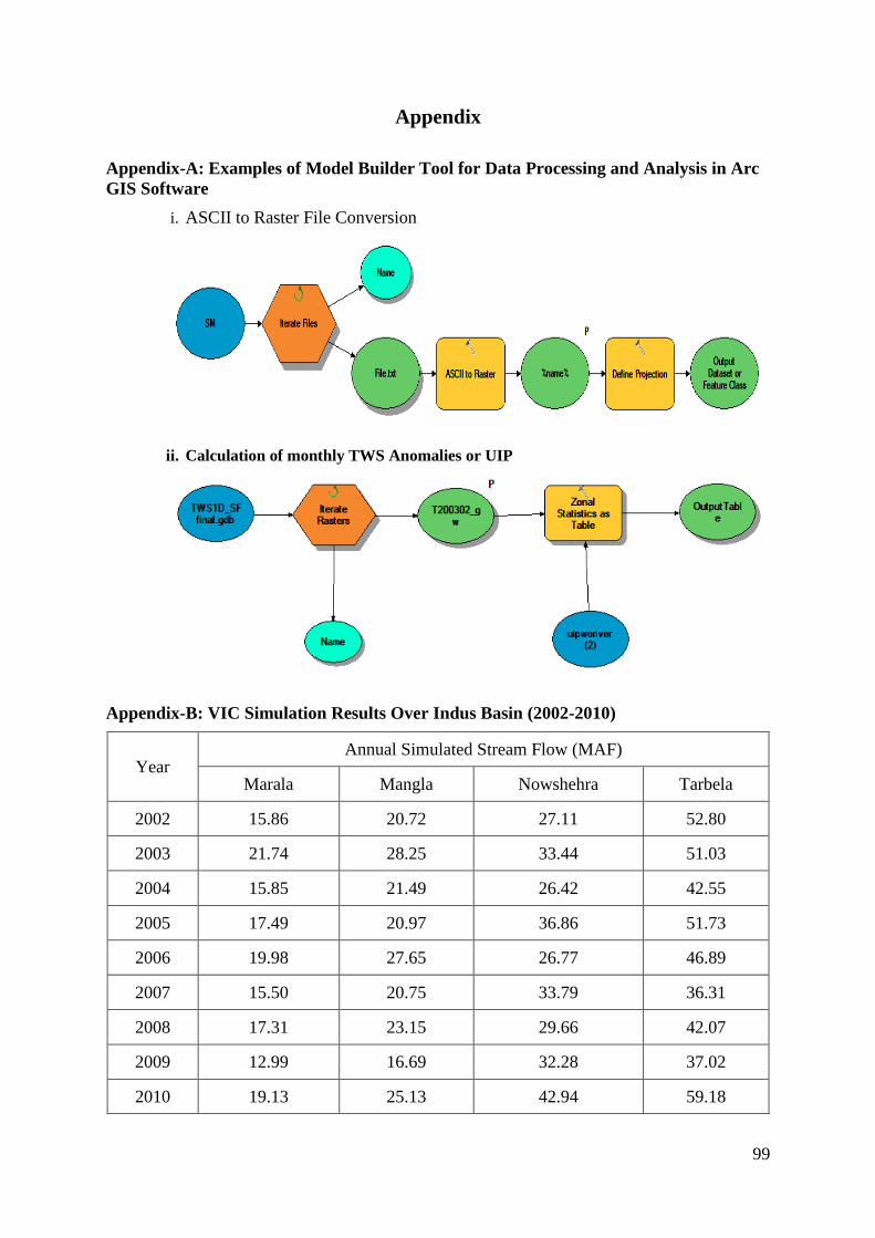
99
Appendix
Appendix-A: Examples of Model Builder Tool for Data Processing and Analysis in Arc
GIS Software
i. ASCII to Raster File Conversion
ii. Calculation of monthly TWS Anomalies or UIP
Appendix-B: VIC Simulation Results Over Indus Basin (2002-2010)
Year Annual Simulated Stream Flow (MAF)
Marala Mangla Nowshehra Tarbela
2002 15.86 20.72 27.11 52.80
2003 21.74 28.25 33.44 51.03
2004 15.85 21.49 26.42 42.55
2005 17.49 20.97 36.86 51.73
2006 19.98 27.65 26.77 46.89
2007 15.50 20.75 33.79 36.31
2008 17.31 23.15 29.66 42.07
2009 12.99 16.69 32.28 37.02
2010 19.13 25.13 42.94 59.18
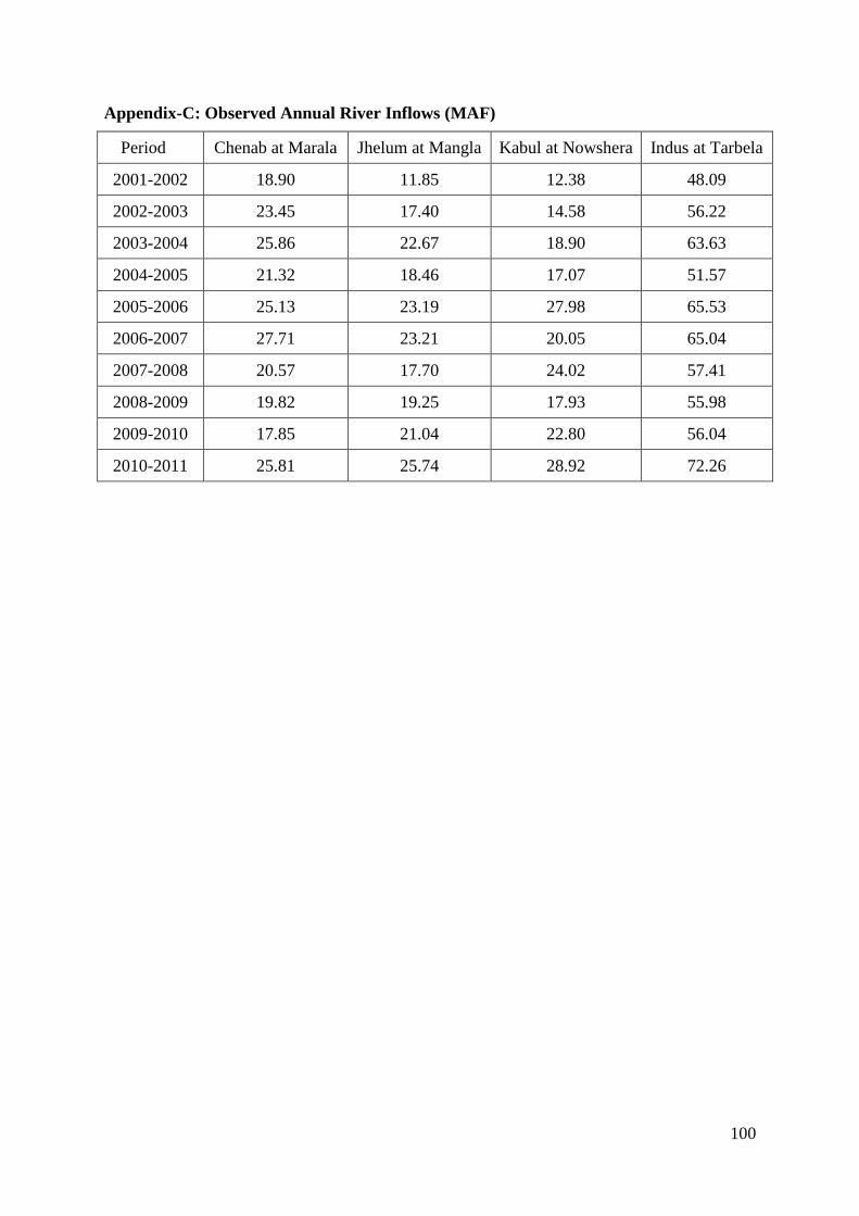
100
Appendix-C: Observed Annual River Inflows (MAF)
Period Chenab at Marala Jhelum at Mangla Kabul at Nowshera Indus at Tarbela
2001-2002 18.90 11.85 12.38 48.09
2002-2003 23.45 17.40 14.58 56.22
2003-2004 25.86 22.67 18.90 63.63
2004-2005 21.32 18.46 17.07 51.57
2005-2006 25.13 23.19 27.98 65.53
2006-2007 27.71 23.21 20.05 65.04
2007-2008 20.57 17.70 24.02 57.41
2008-2009 19.82 19.25 17.93 55.98
2009-2010 17.85 21.04 22.80 56.04
2010-2011 25.81 25.74 28.92 72.26
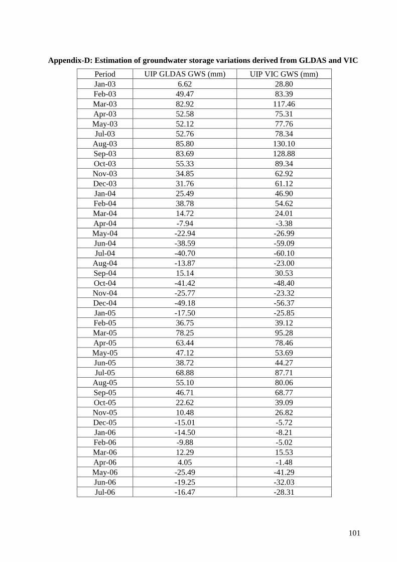
101
Appendix-D: Estimation of groundwater storage variations derived from GLDAS and VIC
Period UIP GLDAS GWS (mm) UIP VIC GWS (mm)
Jan-03 6.62 28.80
Feb-03 49.47 83.39
Mar-03 82.92 117.46
Apr-03 52.58 75.31
May-03 52.12 77.76
Jul-03 52.76 78.34
Aug-03 85.80 130.10
Sep-03 83.69 128.88
Oct-03 55.33 89.34
Nov-03 34.85 62.92
Dec-03 31.76 61.12
Jan-04 25.49 46.90
Feb-04 38.78 54.62
Mar-04 14.72 24.01
Apr-04 -7.94 -3.38
May-04 -22.94 -26.99
Jun-04 -38.59 -59.09
Jul-04 -40.70 -60.10
Aug-04 -13.87 -23.00
Sep-04 15.14 30.53
Oct-04 -41.42 -48.40
Nov-04 -25.77 -23.32
Dec-04 -49.18 -56.37
Jan-05 -17.50 -25.85
Feb-05 36.75 39.12
Mar-05 78.25 95.28
Apr-05 63.44 78.46
May-05 47.12 53.69
Jun-05 38.72 44.27
Jul-05 68.88 87.71
Aug-05 55.10 80.06
Sep-05 46.71 68.77
Oct-05 22.62 39.09
Nov-05 10.48 26.82
Dec-05 -15.01 -5.72
Jan-06 -14.50 -8.21
Feb-06 -9.88 -5.02
Mar-06 12.29 15.53
Apr-06 4.05 -1.48
May-06 -25.49 -41.29
Jun-06 -19.25 -32.03
Jul-06 -16.47 -28.31
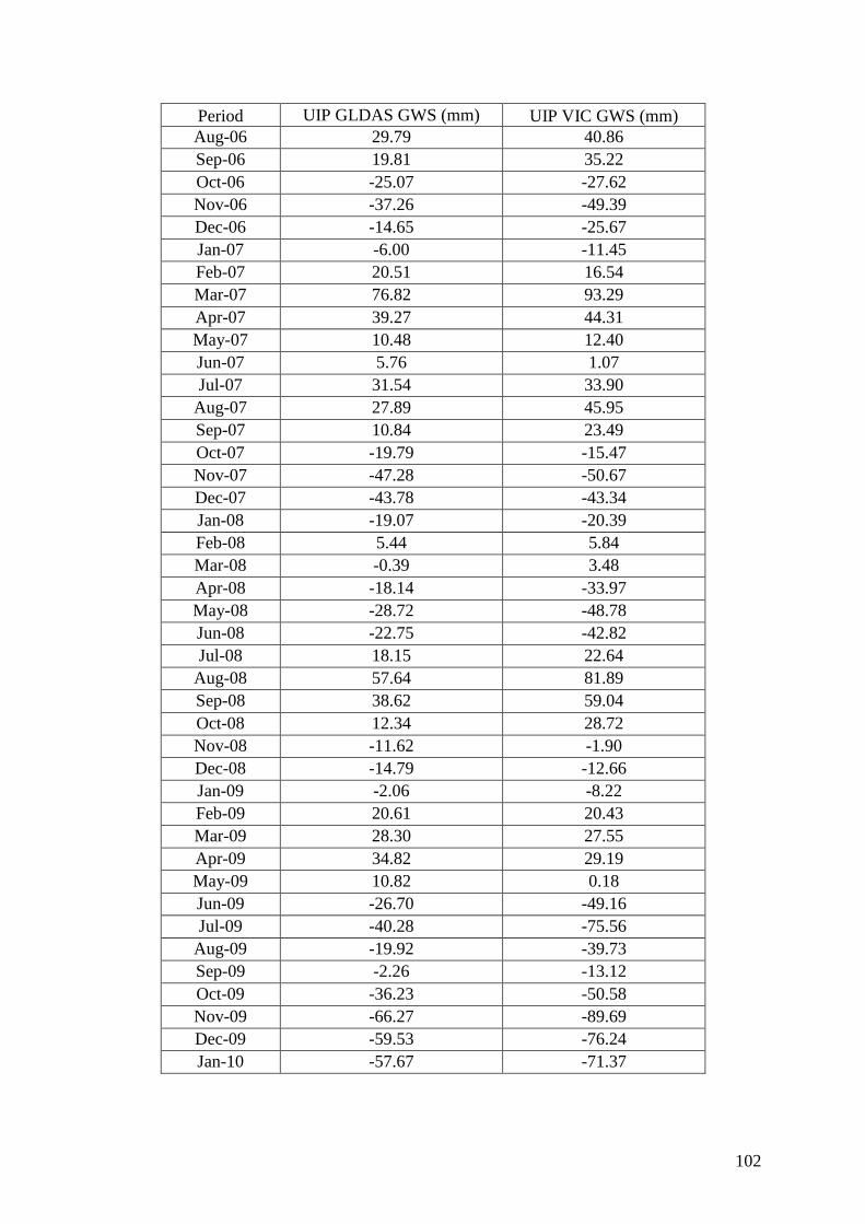
102
Period UIP GLDAS GWS (mm) UIP VIC GWS (mm)
Aug-06 29.79 40.86
Sep-06 19.81 35.22
Oct-06 -25.07 -27.62
Nov-06 -37.26 -49.39
Dec-06 -14.65 -25.67
Jan-07 -6.00 -11.45
Feb-07 20.51 16.54
Mar-07 76.82 93.29
Apr-07 39.27 44.31
May-07 10.48 12.40
Jun-07 5.76 1.07
Jul-07 31.54 33.90
Aug-07 27.89 45.95
Sep-07 10.84 23.49
Oct-07 -19.79 -15.47
Nov-07 -47.28 -50.67
Dec-07 -43.78 -43.34
Jan-08 -19.07 -20.39
Feb-08 5.44 5.84
Mar-08 -0.39 3.48
Apr-08 -18.14 -33.97
May-08 -28.72 -48.78
Jun-08 -22.75 -42.82
Jul-08 18.15 22.64
Aug-08 57.64 81.89
Sep-08 38.62 59.04
Oct-08 12.34 28.72
Nov-08 -11.62 -1.90
Dec-08 -14.79 -12.66
Jan-09 -2.06 -8.22
Feb-09 20.61 20.43
Mar-09 28.30 27.55
Apr-09 34.82 29.19
May-09 10.82 0.18
Jun-09 -26.70 -49.16
Jul-09 -40.28 -75.56
Aug-09 -19.92 -39.73
Sep-09 -2.26 -13.12
Oct-09 -36.23 -50.58
Nov-09 -66.27 -89.69
Dec-09 -59.53 -76.24
Jan-10 -57.67 -71.37
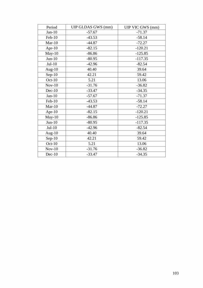
103
Period UIP GLDAS GWS (mm) UIP VIC GWS (mm)
Jan-10 -57.67 -71.37
Feb-10 -43.53 -58.14
Mar-10 -44.87 -72.27
Apr-10 -82.15 -120.21
May-10 -86.86 -125.85
Jun-10 -80.95 -117.35
Jul-10 -42.96 -82.54
Aug-10 40.40 39.64
Sep-10 42.21 59.42
Oct-10 5.21 13.06
Nov-10 -31.76 -36.82
Dec-10 -33.47 -34.35
Jan-10 -57.67 -71.37
Feb-10 -43.53 -58.14
Mar-10 -44.87 -72.27
Apr-10 -82.15 -120.21
May-10 -86.86 -125.85
Jun-10 -80.95 -117.35
Jul-10 -42.96 -82.54
Aug-10 40.40 39.64
Sep-10 42.21 59.42
Oct-10 5.21 13.06
Nov-10 -31.76 -36.82
Dec-10 -33.47 -34.35
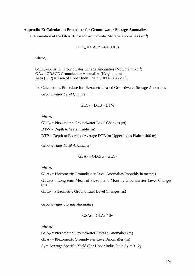
104
Appendix-E: Calculation Procedure for Groundwater Storage Anomalies
a. Estimation of the GRACE based Groundwater Storage Anomalies (km3)
GSEG = GAG * Area (UIP)
where;
GSEG = GRACE Groundwater Storage Anomalies (Volume in km3)
GAG = GRACE Groundwater Anomalies (Height in m)
Area (UIP) = Area of Upper Indus Plain (109,418.35 km2)
b. Calculations Procedure for Piezometric based Groundwater Storage Anomalies
Groundwater Level Change
GLCP = DTB – DTW
where;
GLCP = Piezometric Groundwater Level Changes (m)
DTW = Depth to Water Table (m)
DTB = Depth to Bedrock (Average DTB for Upper Indus Plain = 400 m)
Groundwater Level Anomalies
GLAP = GLCPM – GLCP
where;
GLAP = Piezometric Groundwater Level Anomalies (monthly in meters)
GLCPM = Long term Mean of Piezometric Monthly Groundwater Level Changes
(m)
GLCP = Piezometric Groundwater Level Changes (m)
Groundwater Storage Anomalies
GSAP = GLAP * SY
where;
GSAP = Piezometric Groundwater Storage Anomalies (m)
GLAP = Piezometric Groundwater Level Anomalies (m)
SY = Average Specific Yield (For Upper Indus Plain SY = 0.12)
105
Groundwater Storage Estimation (km3)
GSEP = GSAP * Area (UIP)
where;
GSEP = Piezometric Groundwater Storage Anomalies (Volume in km3)
GSAP = Piezometric Groundwater Storage Anomalies (m)
Area (UIP) = Area of Upper Indus Plain (109,418.35 km2)