Satellite Cross comparisonMorisette 1 Satellite LAI Cross Comparison Jeff Morisette, Jeff Privette...
25
Satellite Cross comparison Morisette 1 Satellite LAI Cross Comparison Jeff Morisette, Jeff Privette – MODLAND Validation Eric Vermote – MODIS Surface Reflectance David Roy – MODIS Quality Assurance Alfredo Huete – MODIS NDVI product Outline: High resolution data at EOS Land Validation Core Site Statistical regression analysis, initial results (comparing NDVI from ETM+, MODIS, and AVHRR) Future plans for comparing multiple LAI products
-
Upload
dominic-jessie-hill -
Category
Documents
-
view
221 -
download
0
Transcript of Satellite Cross comparisonMorisette 1 Satellite LAI Cross Comparison Jeff Morisette, Jeff Privette...
Satellite Cross comparison Morisette1
Satellite LAI Cross Comparison
Jeff Morisette, Jeff Privette – MODLAND ValidationEric Vermote – MODIS Surface Reflectance
David Roy – MODIS Quality AssuranceAlfredo Huete – MODIS NDVI product
Satellite LAI Cross Comparison
Jeff Morisette, Jeff Privette – MODLAND ValidationEric Vermote – MODIS Surface Reflectance
David Roy – MODIS Quality AssuranceAlfredo Huete – MODIS NDVI product
Outline:
High resolution data at EOS Land Validation Core Site
Statistical regression analysis, initial results(comparing NDVI from ETM+, MODIS, and AVHRR)
Future plans for comparing multiple LAI products
Satellite Cross comparison Morisette2
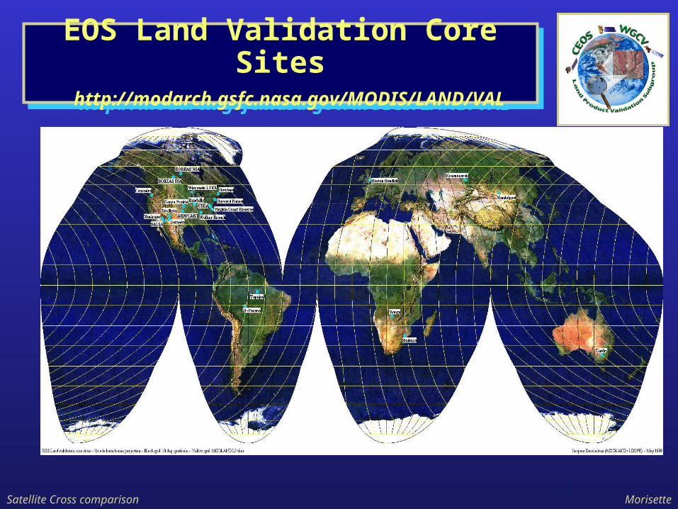
EOS Land Validation Core Sites
http://modarch.gsfc.nasa.gov/MODIS/LAND/VA
L
EOS Land Validation Core Sites
http://modarch.gsfc.nasa.gov/MODIS/LAND/VA
L
Satellite Cross comparison Morisette3
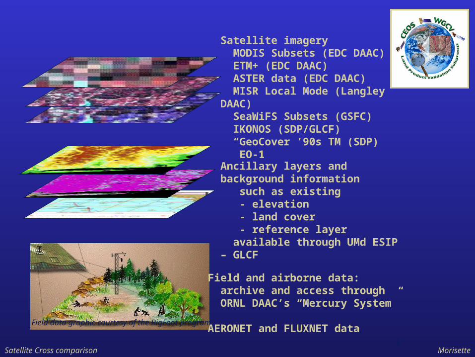
Satellite imagery MODIS Subsets (EDC DAAC) ETM+ (EDC DAAC) ASTER data (EDC DAAC) MISR Local Mode (Langley DAAC) SeaWiFS Subsets (GSFC) IKONOS (SDP/GLCF) “GeoCover ’90s TM (SDP) EO-1 Ancillary layers and background information such as existing - elevation - land cover - reference layer available through UMd ESIP – GLCF
Field data graphic courtesy of the BigFoot program
Field and airborne data: archive and access through ORNL DAAC’s “Mercury System”
AERONET and FLUXNET data
Satellite Cross comparison Morisette4
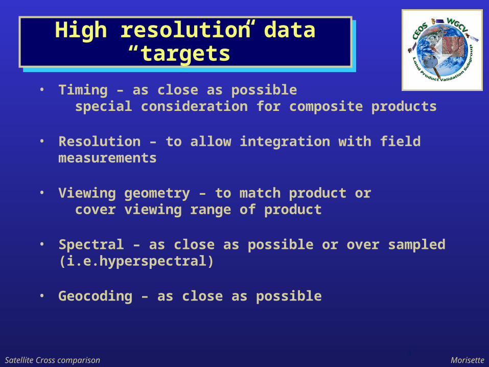
High resolution data“targets”
High resolution data“targets”
• Timing – as close as possible special consideration for composite products
• Resolution – to allow integration with field measurements
• Viewing geometry – to match product or cover viewing range of product
• Spectral – as close as possible or over sampled (i.e.hyperspectral)
• Geocoding – as close as possible
Satellite Cross comparison Morisette5
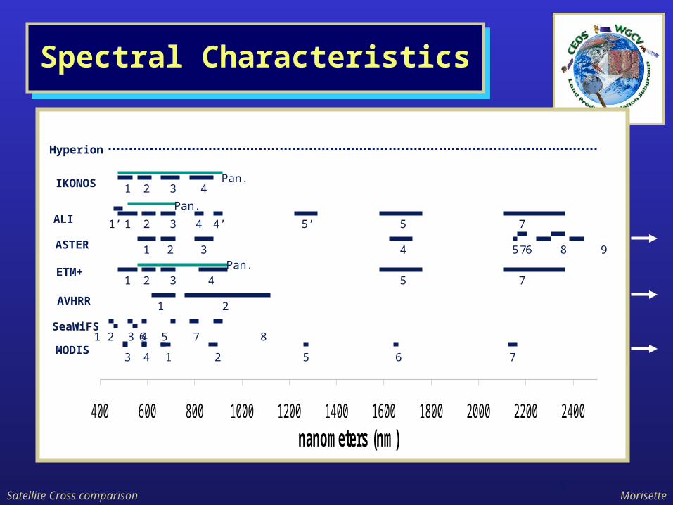
Spectral CharacteristicsSpectral Characteristics
400 600 800 1000 1200 1400 1600 1800 2000 2200 2400
nanometers (nm)
5 6 7
5 7
4 5 6 7 8 9
5 75’
1 243
1 2 3 4 5 6 7 8
1 2
1 2 43Pan.
1 2 3
1 2 43 4’1’
Pan.
Pan.1 2 43
MODIS
SeaWiFS
AVHRR
ETM+
ASTER
ALI
IKONOS
Hyperion
Satellite Cross comparison Morisette6
AR
M/C
AR
T
Bar
ton
Ben
dish
Bon
dvil
le,I
L
BO
RE
AS,
NSA
BO
RE
AS
SSA
/B
ER
MS
Cas
cade
sLT
ER
Har
vard
For
est
How
land
Ji-
Par
ana
Jor
nada
LT
ER
Kon
za P
rari
e
Kra
snoy
arsk
Man
dolg
obi
Mar
icop
a A
g.
Mon
gu
SA
LSA
Sev
ille
ta L
TE
R
Sku
kuza
Tap
ajos
Uar
dry
USD
A A
RS
VC
R
Wal
ker
Bra
nch
Wis
c.P
ark
Fal
ls
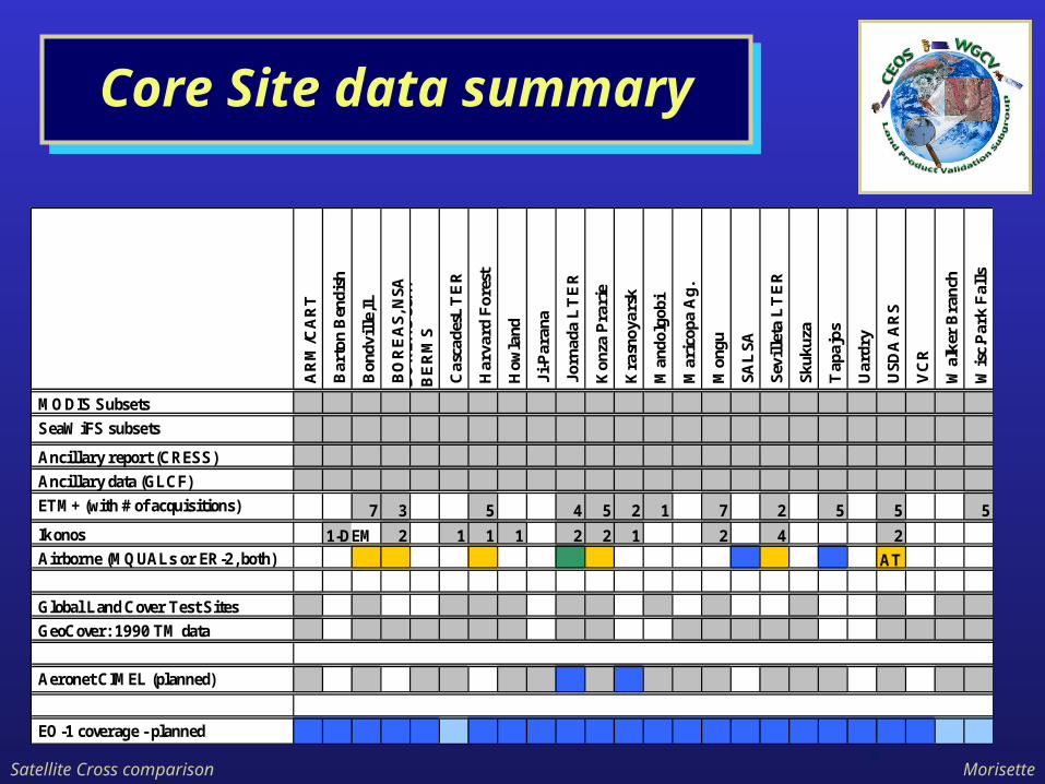
MODIS Subsets
SeaWiFS subsets
Ancillary report (CRESS)
Ancillary data (GLCF)
ETM+ (with # of acquisitions) 7 3 5 4 5 2 1 7 2 5 5 5
Ikonos 1-DEM 2 1 1 1 2 2 1 2 4 2 Airborne (MQUALs or ER-2, both) AT
Global Land Cover Test Sites
GeoCover: 1990 TM data
Aeronet CIMEL (planned)
EO-1 coverage - planned
Core Site data summary
Core Site data summary
Satellite Cross comparison Morisette7
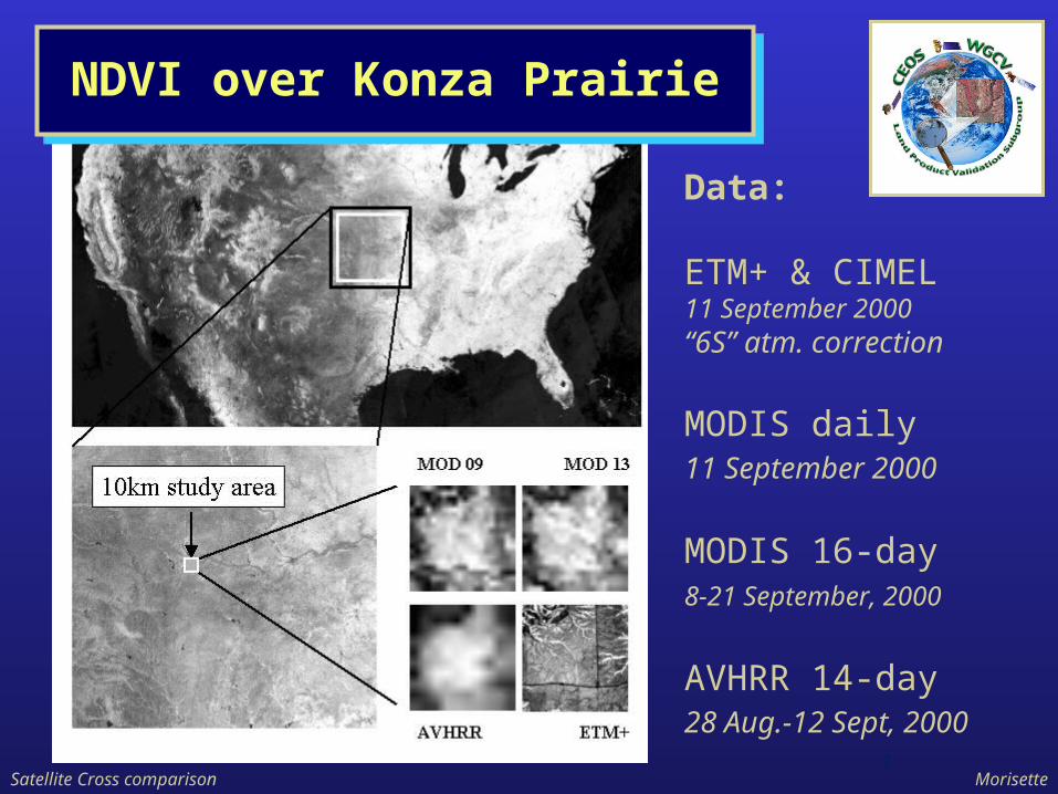
NDVI over Konza PrairieNDVI over Konza Prairie
Data:
ETM+ & CIMEL11 September 2000“6S” atm. correction
MODIS daily11 September 2000
MODIS 16-day 8-21 September, 2000
AVHRR 14-day28 Aug.-12 Sept, 2000
Satellite Cross comparison Morisette8
Correlative Analysis:Issues
Correlative Analysis:Issues
• Typical inference is based on a null hypothesis of “no correlation” (i.e. correlation = 0, regression slope term = 0)
• Inference on correlation assume, among other things, independent data
• Correlation and R2 alone do not tell the whole story
• Regression analysis includes several assumptions
• Subset size and location will influence results
Satellite Cross comparison Morisette9
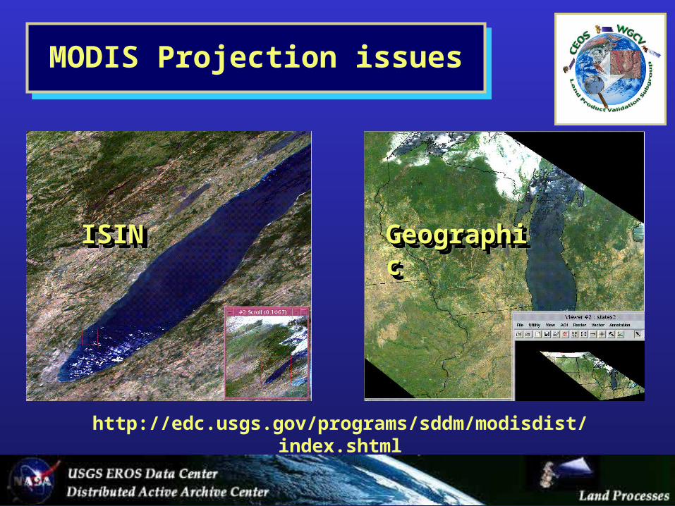
http://edc.usgs.gov/programs/sddm/modisdist/index.shtml
ISINISINISINISIN GeographicGeographicGeographicGeographic
MODIS Projection issuesMODIS Projection issues
Satellite Cross comparison Morisette10
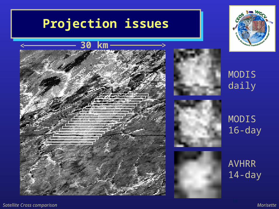
Projection issuesProjection issues
30 km
MODIS daily
MODIS 16-day
AVHRR 14-day
Satellite Cross comparison Morisette11
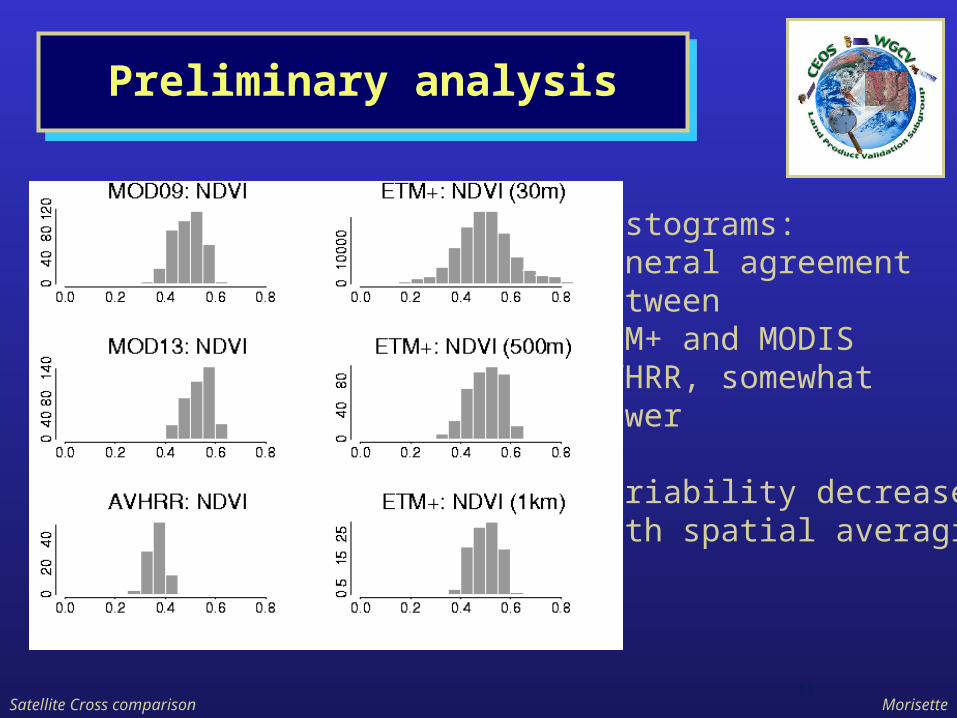
Preliminary analysisPreliminary analysis
Histograms:General agreement between ETM+ and MODISAVHRR, somewhatlower
Variability decreaseswith spatial averaging
Satellite Cross comparison Morisette12
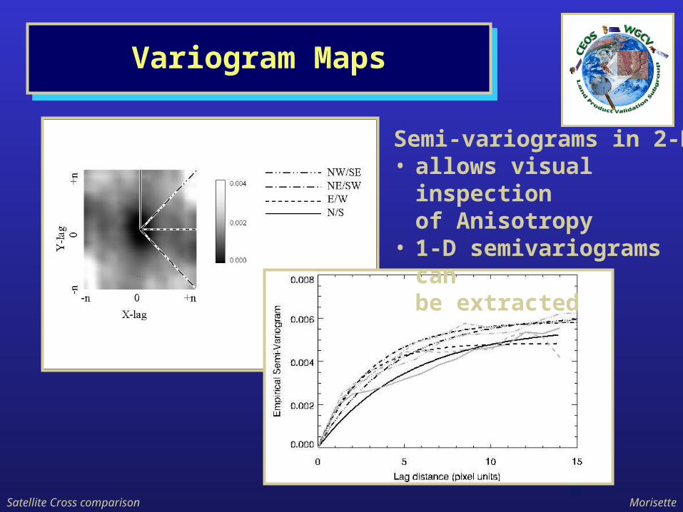
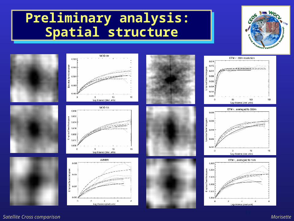
Variogram MapsVariogram Maps
Semi-variograms in 2-D• allows visual inspection
of Anisotropy• 1-D semivariograms can
be extracted
Satellite Cross comparison Morisette13
Preliminary analysis: Spatial structure
Preliminary analysis: Spatial structure
Satellite Cross comparison Morisette14
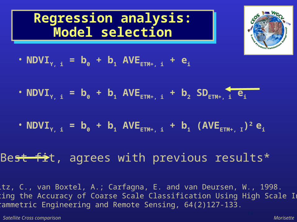
Regression analysis:Model selection
Regression analysis:Model selection
• NDVIY, i = b0 + b1 AVEETM+, i + ei
• NDVIY, i = b0 + b1 AVEETM+, i + b2 SDETM+, i ei
• NDVIY, i = b0 + b1 AVEETM+, i + b1 (AVEETM+, I)2 ei
Best fit, agrees with previous results*
* Klökitz, C., van Boxtel, A.; Carfagna, E. and van Deursen, W., 1998. Estimating the Accuracy of Coarse Scale Classification Using High Scale Information. Photogrammetric Engineering and Remote Sensing, 64(2)127-133.
Satellite Cross comparison Morisette15
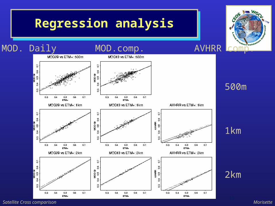
Regression analysisRegression analysis
500m
1km
2km
MOD. Daily MOD.comp. AVHRR comp.
Satellite Cross comparison Morisette16
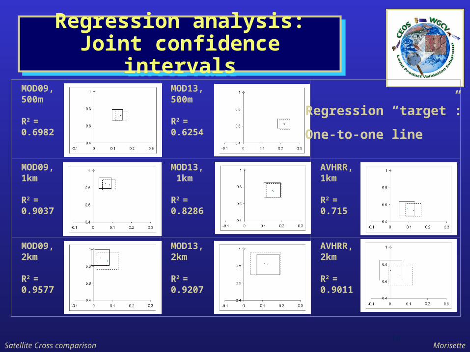
Regression analysis:Joint confidence intervals
Regression analysis:Joint confidence intervals
MOD09, 500m
R2 =0.6982
MOD13, 500m
R2 =0.6254
MOD09, 1km
R2 =0.9037
MOD13, 1km
R2 =0.8286
AVHRR, 1km
R2 =0.715
MOD09, 2km
R2 =0.9577
MOD13, 2km
R2 =0.9207
AVHRR, 2km
R2 =0.9011
Regression “target”:
One-to-one line
Satellite Cross comparison Morisette17
Checking Regression assumptions
Checking Regression assumptions
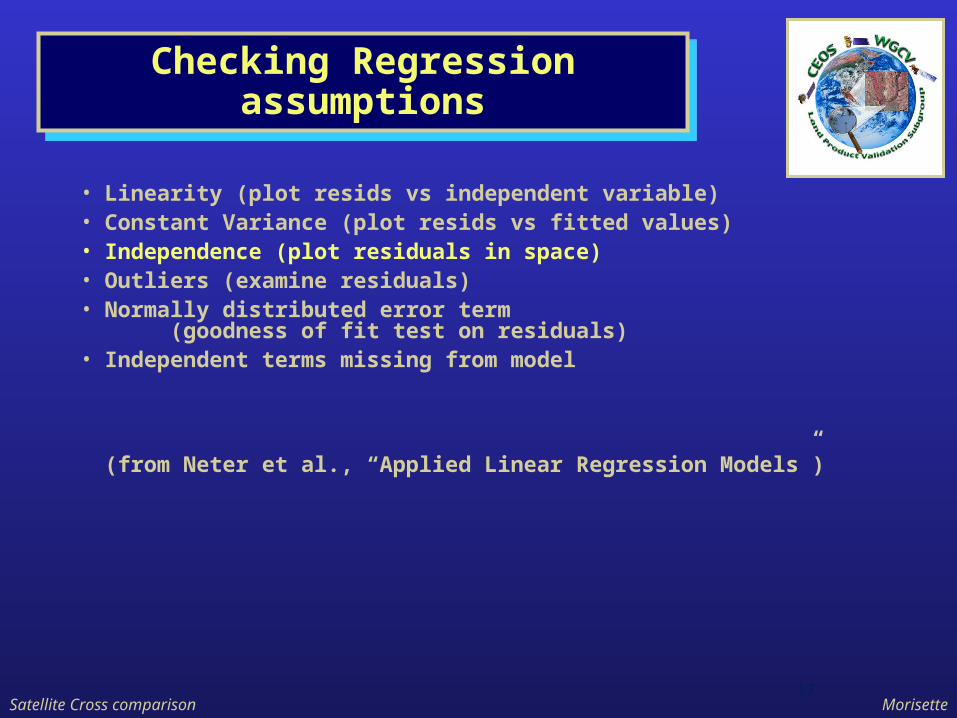
• Linearity (plot resids vs independent variable)• Constant Variance (plot resids vs fitted values)• Independence (plot residuals in space)• Outliers (examine residuals)• Normally distributed error term
(goodness of fit test on residuals)• Independent terms missing from model
(from Neter et al., “Applied Linear Regression Models”)
Satellite Cross comparison Morisette18
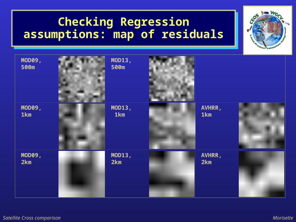
Checking Regression assumptions: map of residuals
Checking Regression assumptions: map of residuals
MOD09, 500m
MOD13, 500m
MOD09, 1km
MOD13, 1km
AVHRR, 1km
MOD09, 2km
MOD13, 2km
AVHRR, 2km
Satellite Cross comparison Morisette19
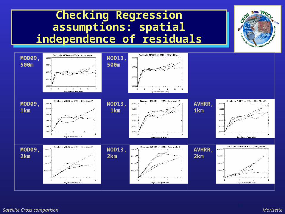
Checking Regression assumptions: spatial
independence of residuals
Checking Regression assumptions: spatial
independence of residuals
MOD09, 500m
MOD13, 500m
MOD09, 1km
MOD13, 1km
AVHRR, 1km
MOD09, 2km
MOD13, 2km
AVHRR, 2km
Satellite Cross comparison Morisette20
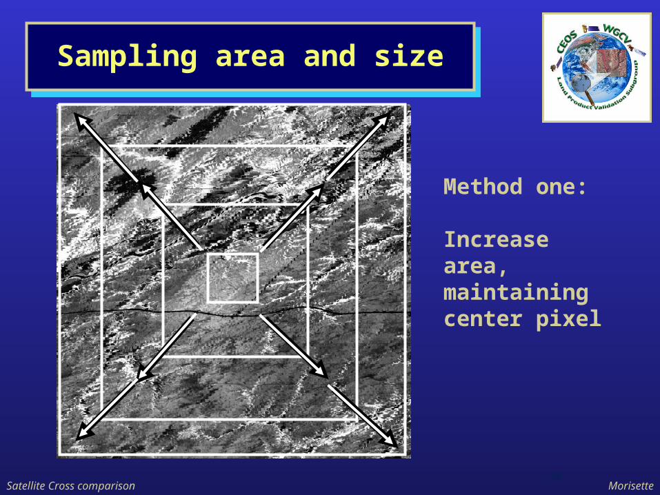
Sampling area and sizeSampling area and size
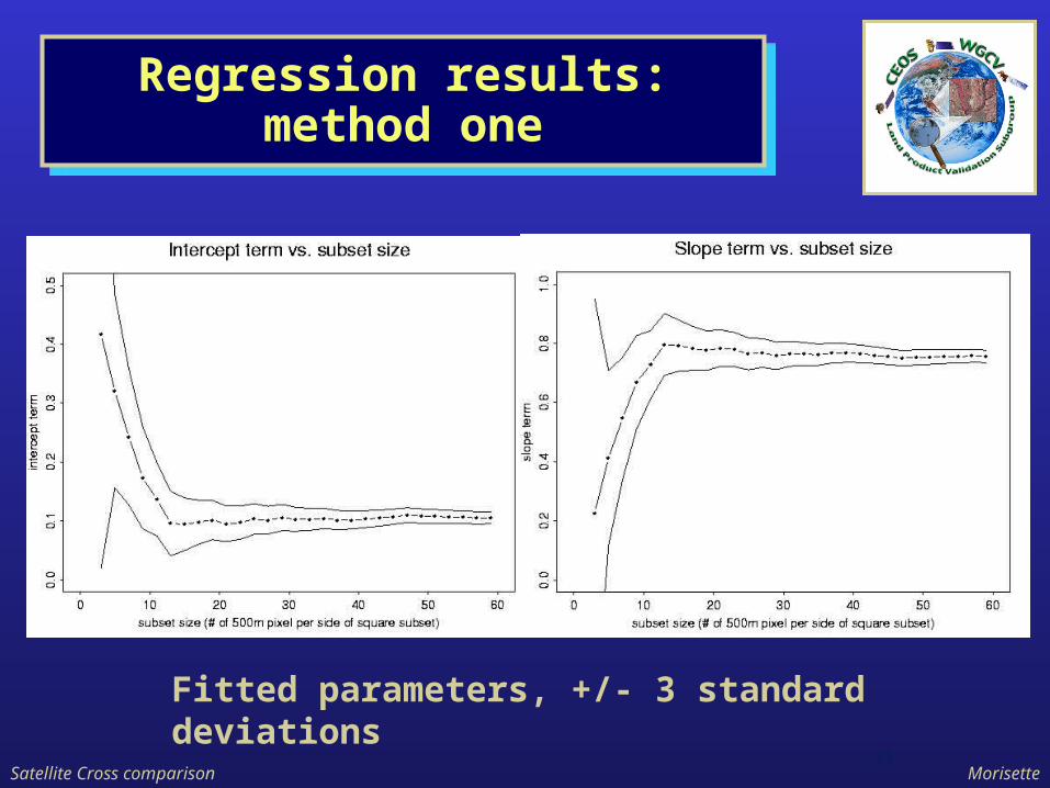
Method one:
Increase area, maintainingcenter pixel
Satellite Cross comparison Morisette21
Regression results:method one
Regression results:method one
Fitted parameters, +/- 3 standard deviations
Satellite Cross comparison Morisette22
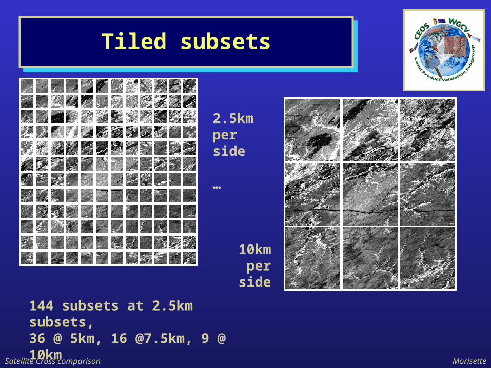
Tiled subsetsTiled subsets
2.5km per side
…
10kmper side
144 subsets at 2.5km subsets, 36 @ 5km, 16 @7.5km, 9 @ 10km
Satellite Cross comparison Morisette23
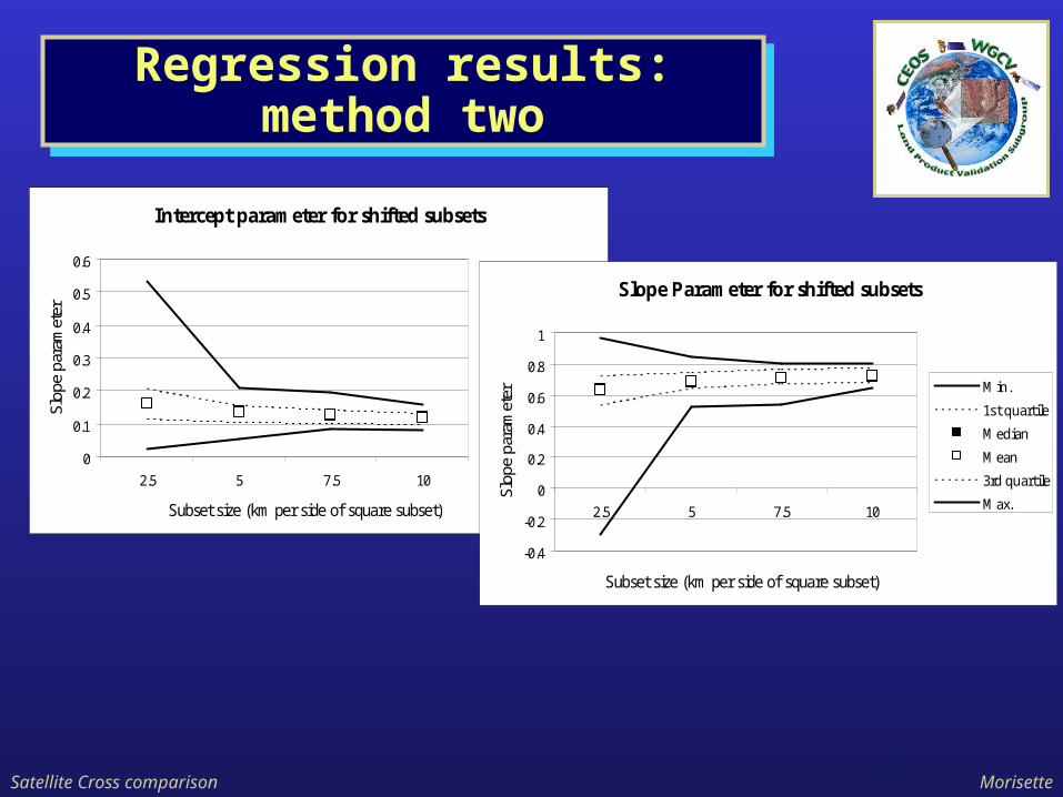
Regression results:method two
Regression results:method two
Intercept parameter for shifted subsets
0
0.1
0.2
0.3
0.4
0.5
0.6
2.5 5 7.5 10
Subset size (km per side of square subset)
Slop
e pa
ram
eter
Min.
1st quartile
Median
Mean
3rd quartile
Max.
Slope Parameter for shifted subsets
-0.4
-0.2
0
0.2
0.4
0.6
0.8
1
2.5 5 7.5 10
Subset size (km per side of square subset)
Slop
e pa
ram
eter
Min.
1st quartile
Median
Mean
3rd quartile
Max.
Satellite Cross comparison Morisette24
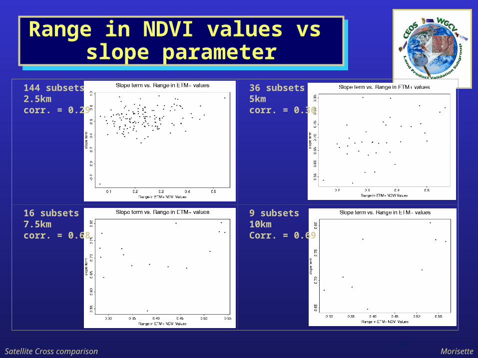
Range in NDVI values vs slope parameter
Range in NDVI values vs slope parameter
144 subsets2.5kmcorr. = 0.29
36 subsets5kmcorr. = 0.36
16 subsets7.5kmcorr. = 0.68
9 subsets 10km Corr. = 0.69
Satellite Cross comparison Morisette25
Conclusion from correlative analysis
Conclusion from correlative analysis
• Regression analysis and the joint confidence intervals on the slope and intercept terms provide a meaningful summary for validation analysis.
• In comparing two coarse resolution products, the comparison should be made with both products at the same resolution.
• Here, the daily MODIS product is the most directly related to the averaged ETM+ data; which implies the importance of considering temporal composite issues.
• Subset location and size have an affect on the regression parameters. For this area, a 10km subset provided a stable subset size.
• These statistical methods can be directly applied to comparing high and coarse resolution LAI products.