Sashelp Data Sets - SAS Supportsupport.sas.com/documentation/onlinedoc/stat/131/sashelp.pdf ·...
28
SAS/STAT ® 13.1 User’s Guide Sashelp Data Sets
-
Upload
truongdiep -
Category
Documents
-
view
232 -
download
0
Transcript of Sashelp Data Sets - SAS Supportsupport.sas.com/documentation/onlinedoc/stat/131/sashelp.pdf ·...
SAS/STAT® 13.1 User’s GuideSashelp Data Sets
This document is an individual chapter from SAS/STAT® 13.1 User’s Guide.
The correct bibliographic citation for the complete manual is as follows: SAS Institute Inc. 2013. SAS/STAT® 13.1 User’s Guide.Cary, NC: SAS Institute Inc.
Copyright © 2013, SAS Institute Inc., Cary, NC, USA
All rights reserved. Produced in the United States of America.
For a hard-copy book: No part of this publication may be reproduced, stored in a retrieval system, or transmitted, in any form or byany means, electronic, mechanical, photocopying, or otherwise, without the prior written permission of the publisher, SAS InstituteInc.
For a web download or e-book: Your use of this publication shall be governed by the terms established by the vendor at the timeyou acquire this publication.
The scanning, uploading, and distribution of this book via the Internet or any other means without the permission of the publisher isillegal and punishable by law. Please purchase only authorized electronic editions and do not participate in or encourage electronicpiracy of copyrighted materials. Your support of others’ rights is appreciated.
U.S. Government License Rights; Restricted Rights: The Software and its documentation is commercial computer softwaredeveloped at private expense and is provided with RESTRICTED RIGHTS to the United States Government. Use, duplication ordisclosure of the Software by the United States Government is subject to the license terms of this Agreement pursuant to, asapplicable, FAR 12.212, DFAR 227.7202-1(a), DFAR 227.7202-3(a) and DFAR 227.7202-4 and, to the extent required under U.S.federal law, the minimum restricted rights as set out in FAR 52.227-19 (DEC 2007). If FAR 52.227-19 is applicable, this provisionserves as notice under clause (c) thereof and no other notice is required to be affixed to the Software or documentation. TheGovernment’s rights in Software and documentation shall be only those set forth in this Agreement.
SAS Institute Inc., SAS Campus Drive, Cary, North Carolina 27513-2414.
December 2013
SAS provides a complete selection of books and electronic products to help customers use SAS® software to its fullest potential. Formore information about our offerings, visit support.sas.com/bookstore or call 1-800-727-3228.
SAS® and all other SAS Institute Inc. product or service names are registered trademarks or trademarks of SAS Institute Inc. in theUSA and other countries. ® indicates USA registration.
Other brand and product names are trademarks of their respective companies.
SAS and all other SAS Institute Inc. product or service names are registered trademarks or trademarks of SAS Institute Inc. in the USA and other countries. ® indicates USA registration. Other brand and product names are trademarks of their respective companies. © 2013 SAS Institute Inc. All rights reserved. S107969US.0613
Discover all that you need on your journey to knowledge and empowerment.
support.sas.com/bookstorefor additional books and resources.
Gain Greater Insight into Your SAS® Software with SAS Books.

Appendix B
Sashelp Data Sets
ContentsOverview of Sashelp Data Sets . . . . . . . . . . . . . . . . . . . . . . . . . . . . . . . . . 9131Baseball Data . . . . . . . . . . . . . . . . . . . . . . . . . . . . . . . . . . . . . . . . . . 9133Bone Marrow Transplant Data . . . . . . . . . . . . . . . . . . . . . . . . . . . . . . . . . 9135Birth Weight Data . . . . . . . . . . . . . . . . . . . . . . . . . . . . . . . . . . . . . . . . 9137Class Data . . . . . . . . . . . . . . . . . . . . . . . . . . . . . . . . . . . . . . . . . . . . 9138Comet Data . . . . . . . . . . . . . . . . . . . . . . . . . . . . . . . . . . . . . . . . . . . 9139El Niño–Southern Oscillation Data . . . . . . . . . . . . . . . . . . . . . . . . . . . . . . . 9140Finland’s Lake Laengelmaevesi Fish Catch Data . . . . . . . . . . . . . . . . . . . . . . . 9141Exhaust Emissions Data . . . . . . . . . . . . . . . . . . . . . . . . . . . . . . . . . . . . 9143Fisher (1936) Iris Data . . . . . . . . . . . . . . . . . . . . . . . . . . . . . . . . . . . . . 9145Junk E-Mail Data . . . . . . . . . . . . . . . . . . . . . . . . . . . . . . . . . . . . . . . . 9146Leukemia Data Sets . . . . . . . . . . . . . . . . . . . . . . . . . . . . . . . . . . . . . . . 9149Margarine Data . . . . . . . . . . . . . . . . . . . . . . . . . . . . . . . . . . . . . . . . . 9151Coal Seam Thickness Data . . . . . . . . . . . . . . . . . . . . . . . . . . . . . . . . . . . 9152Flying Mileages between Five US Cities Data . . . . . . . . . . . . . . . . . . . . . . . . . 9153References . . . . . . . . . . . . . . . . . . . . . . . . . . . . . . . . . . . . . . . . . . . 9154
Overview of Sashelp Data SetsSAS provides more than 200 data sets in the Sashelp library. These data sets are available for you to use forexamples and for testing code. For example, the following step uses the Sashelp.Class data set:
proc reg data=sashelp.Class;model weight = height;
run; quit;
You do not need to provide a DATA step to use Sashelp data sets.
9132 F Appendix B: Sashelp Data Sets
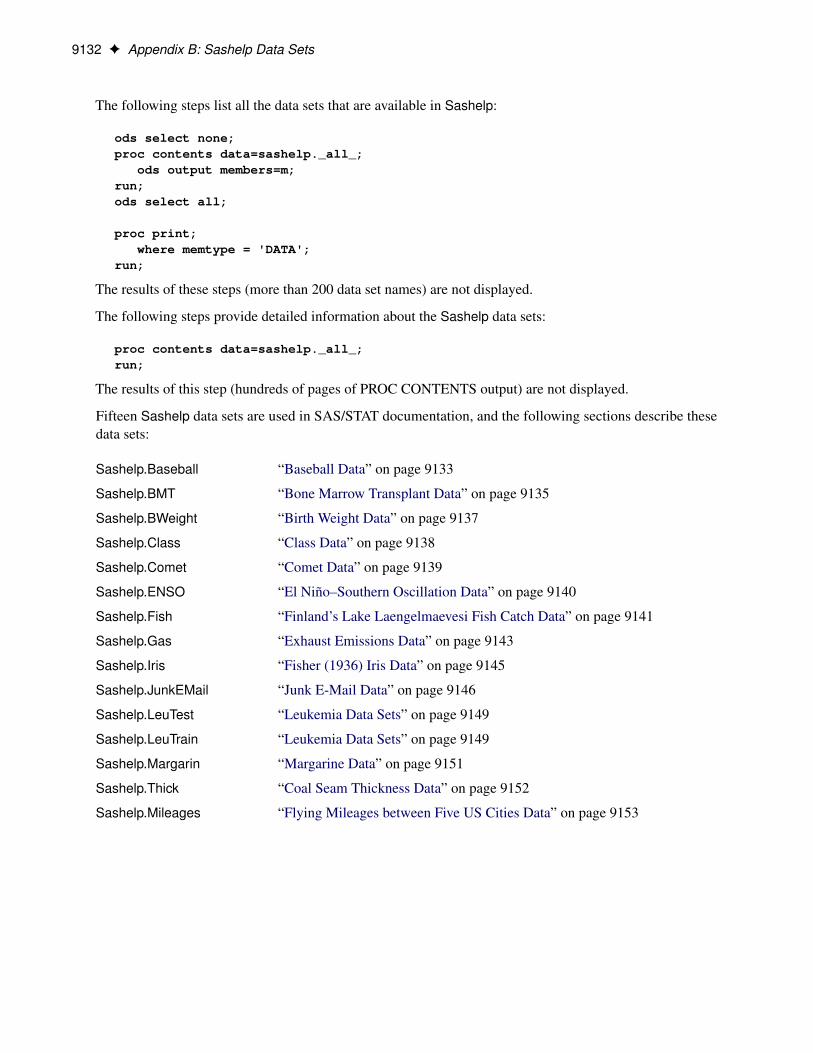
The following steps list all the data sets that are available in Sashelp:
ods select none;proc contents data=sashelp._all_;
ods output members=m;run;ods select all;
proc print;where memtype = 'DATA';
run;
The results of these steps (more than 200 data set names) are not displayed.
The following steps provide detailed information about the Sashelp data sets:
proc contents data=sashelp._all_;run;
The results of this step (hundreds of pages of PROC CONTENTS output) are not displayed.
Fifteen Sashelp data sets are used in SAS/STAT documentation, and the following sections describe thesedata sets:
Sashelp.Baseball “Baseball Data” on page 9133
Sashelp.BMT “Bone Marrow Transplant Data” on page 9135
Sashelp.BWeight “Birth Weight Data” on page 9137
Sashelp.Class “Class Data” on page 9138
Sashelp.Comet “Comet Data” on page 9139
Sashelp.ENSO “El Niño–Southern Oscillation Data” on page 9140
Sashelp.Fish “Finland’s Lake Laengelmaevesi Fish Catch Data” on page 9141
Sashelp.Gas “Exhaust Emissions Data” on page 9143
Sashelp.Iris “Fisher (1936) Iris Data” on page 9145
Sashelp.JunkEMail “Junk E-Mail Data” on page 9146
Sashelp.LeuTest “Leukemia Data Sets” on page 9149
Sashelp.LeuTrain “Leukemia Data Sets” on page 9149
Sashelp.Margarin “Margarine Data” on page 9151
Sashelp.Thick “Coal Seam Thickness Data” on page 9152
Sashelp.Mileages “Flying Mileages between Five US Cities Data” on page 9153

Baseball Data F 9133
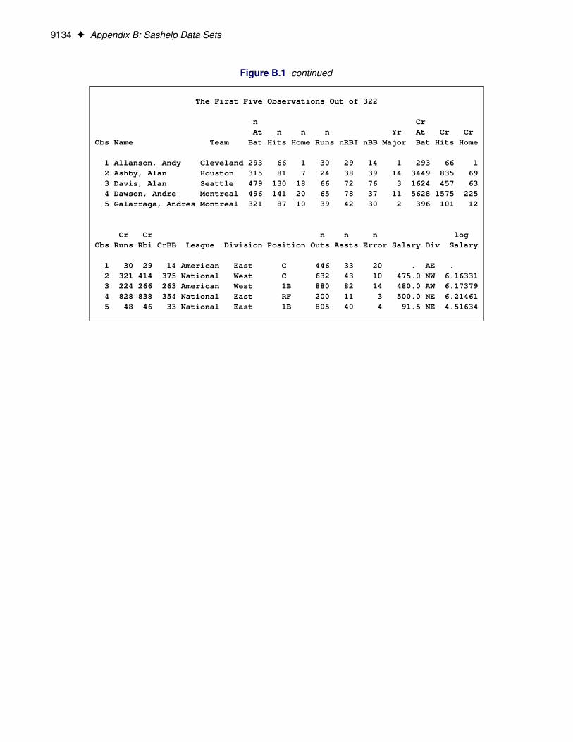
Baseball DataThe Sashelp.Baseball data set contains salary and performance information for Major League Baseballplayers (excluding pitchers) who played at least one game in both the 1986 and 1987 seasons. The salariesare for the 1987 season, and the performance measures are from the 1986 season. The following steps displayinformation about the Sashelp.Baseball data set and create Figure B.1:
title 'Baseball Data';proc contents data=sashelp.Baseball varnum;
ods select position;run;
title 'The First Five Observations Out of 322';proc print data=sashelp.Baseball(obs=5);run;
Figure B.1 Baseball Data
Baseball Data
Variables in Creation Order
# Variable Type Len Label
1 Name Char 18 Player's Name2 Team Char 14 Team at the End of 19863 nAtBat Num 8 Times at Bat in 19864 nHits Num 8 Hits in 19865 nHome Num 8 Home Runs in 19866 nRuns Num 8 Runs in 19867 nRBI Num 8 RBIs in 19868 nBB Num 8 Walks in 19869 YrMajor Num 8 Years in the Major Leagues
10 CrAtBat Num 8 Career Times at Bat11 CrHits Num 8 Career Hits12 CrHome Num 8 Career Home Runs13 CrRuns Num 8 Career Runs14 CrRbi Num 8 Career RBIs15 CrBB Num 8 Career Walks16 League Char 8 League at the End of 198617 Division Char 8 Division at the End of 198618 Position Char 8 Position(s) in 198619 nOuts Num 8 Put Outs in 198620 nAssts Num 8 Assists in 198621 nError Num 8 Errors in 198622 Salary Num 8 1987 Salary in $ Thousands23 Div Char 16 League and Division24 logSalary Num 8 Log Salary
9134 F Appendix B: Sashelp Data Sets
Figure B.1 continued
The First Five Observations Out of 322
n CrAt n n n Yr At Cr Cr
Obs Name Team Bat Hits Home Runs nRBI nBB Major Bat Hits Home
1 Allanson, Andy Cleveland 293 66 1 30 29 14 1 293 66 12 Ashby, Alan Houston 315 81 7 24 38 39 14 3449 835 693 Davis, Alan Seattle 479 130 18 66 72 76 3 1624 457 634 Dawson, Andre Montreal 496 141 20 65 78 37 11 5628 1575 2255 Galarraga, Andres Montreal 321 87 10 39 42 30 2 396 101 12
Cr Cr n n n logObs Runs Rbi CrBB League Division Position Outs Assts Error Salary Div Salary
1 30 29 14 American East C 446 33 20 . AE .2 321 414 375 National West C 632 43 10 475.0 NW 6.163313 224 266 263 American West 1B 880 82 14 480.0 AW 6.173794 828 838 354 National East RF 200 11 3 500.0 NE 6.214615 48 46 33 National East 1B 805 40 4 91.5 NE 4.51634
Bone Marrow Transplant Data F 9135
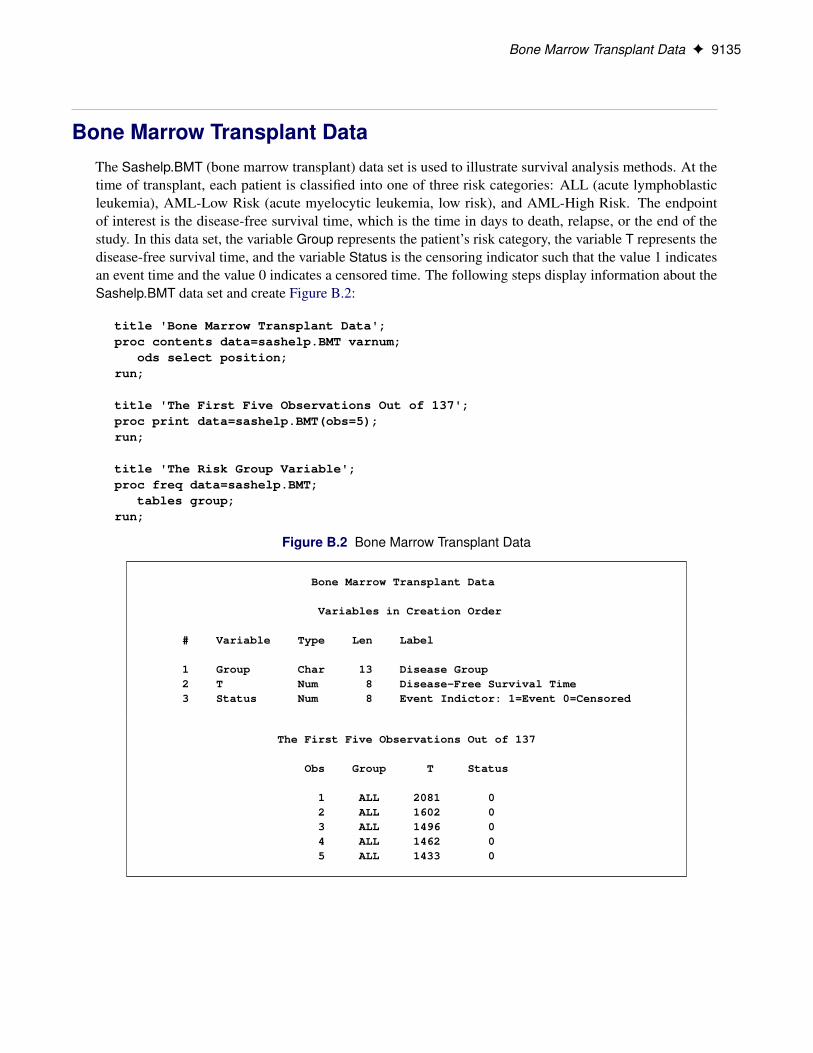
Bone Marrow Transplant DataThe Sashelp.BMT (bone marrow transplant) data set is used to illustrate survival analysis methods. At thetime of transplant, each patient is classified into one of three risk categories: ALL (acute lymphoblasticleukemia), AML-Low Risk (acute myelocytic leukemia, low risk), and AML-High Risk. The endpointof interest is the disease-free survival time, which is the time in days to death, relapse, or the end of thestudy. In this data set, the variable Group represents the patient’s risk category, the variable T represents thedisease-free survival time, and the variable Status is the censoring indicator such that the value 1 indicatesan event time and the value 0 indicates a censored time. The following steps display information about theSashelp.BMT data set and create Figure B.2:
title 'Bone Marrow Transplant Data';proc contents data=sashelp.BMT varnum;
ods select position;run;
title 'The First Five Observations Out of 137';proc print data=sashelp.BMT(obs=5);run;
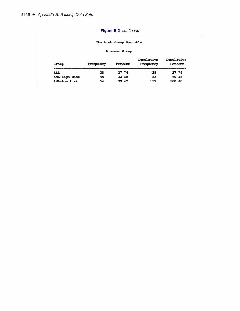
title 'The Risk Group Variable';proc freq data=sashelp.BMT;
tables group;run;
Figure B.2 Bone Marrow Transplant Data
Bone Marrow Transplant Data
Variables in Creation Order
# Variable Type Len Label
1 Group Char 13 Disease Group2 T Num 8 Disease-Free Survival Time3 Status Num 8 Event Indictor: 1=Event 0=Censored
The First Five Observations Out of 137
Obs Group T Status
1 ALL 2081 02 ALL 1602 03 ALL 1496 04 ALL 1462 05 ALL 1433 0
9136 F Appendix B: Sashelp Data Sets
Figure B.2 continued
The Risk Group Variable
Disease Group
Cumulative CumulativeGroup Frequency Percent Frequency Percent------------------------------------------------------------------ALL 38 27.74 38 27.74AML-High Risk 45 32.85 83 60.58AML-Low Risk 54 39.42 137 100.00

Birth Weight Data F 9137
Birth Weight DataThe Sashelp.BWeight data set provides 1997 birth weight data from National Center for Health Statistics.The data record live, singleton births to mothers between the ages of 18 and 45 in the United States who wereclassified as black or white. The following steps display information about the Sashelp.BWeight data set andcreate Figure B.3:
title 'Birth Weight Data';proc contents data=sashelp.BWeight varnum;
ods select position;run;
title 'The First Five Observations Out of 50,000';proc print data=sashelp.BWeight(obs=5);run;
Figure B.3 Birth Weight Data
Birth Weight Data
Variables in Creation Order
# Variable Type Len Label
1 Weight Num 8 Infant Birth Weight2 Black Num 8 Black Mother3 Married Num 8 Married Mother4 Boy Num 8 Baby Boy5 MomAge Num 8 Mother's Age6 MomSmoke Num 8 Smoking Mother7 CigsPerDay Num 8 Cigarettes Per Day8 MomWtGain Num 8 Mother's Pregnancy Weight Gain9 Visit Num 8 Prenatal Visit
10 MomEdLevel Num 8 Mother's Education Level
The First Five Observations Out of 50,000
Mom MomMom Mom Cigs Wt Ed
Obs Weight Black Married Boy Age Smoke PerDay Gain Visit Level
1 4111 0 1 1 -3 0 0 -16 1 02 3997 0 1 0 1 0 0 2 3 23 3572 0 1 1 0 0 0 -3 3 04 1956 0 1 1 -1 0 0 -5 3 25 3515 0 1 1 -6 0 0 -20 3 0
9138 F Appendix B: Sashelp Data Sets
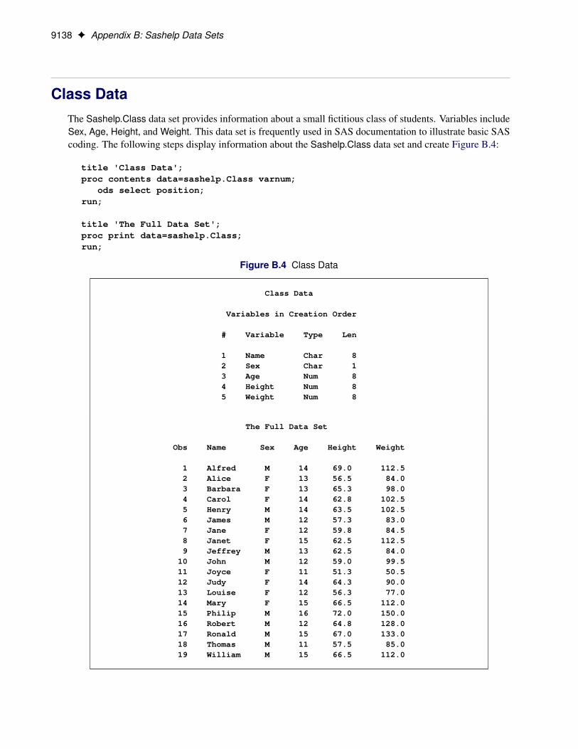
Class DataThe Sashelp.Class data set provides information about a small fictitious class of students. Variables includeSex, Age, Height, and Weight. This data set is frequently used in SAS documentation to illustrate basic SAScoding. The following steps display information about the Sashelp.Class data set and create Figure B.4:
title 'Class Data';proc contents data=sashelp.Class varnum;
ods select position;run;
title 'The Full Data Set';proc print data=sashelp.Class;run;
Figure B.4 Class Data
Class Data
Variables in Creation Order
# Variable Type Len
1 Name Char 82 Sex Char 13 Age Num 84 Height Num 85 Weight Num 8
The Full Data Set
Obs Name Sex Age Height Weight
1 Alfred M 14 69.0 112.52 Alice F 13 56.5 84.03 Barbara F 13 65.3 98.04 Carol F 14 62.8 102.55 Henry M 14 63.5 102.56 James M 12 57.3 83.07 Jane F 12 59.8 84.58 Janet F 15 62.5 112.59 Jeffrey M 13 62.5 84.0
10 John M 12 59.0 99.511 Joyce F 11 51.3 50.512 Judy F 14 64.3 90.013 Louise F 12 56.3 77.014 Mary F 15 66.5 112.015 Philip M 16 72.0 150.016 Robert M 12 64.8 128.017 Ronald M 15 67.0 133.018 Thomas M 11 57.5 85.019 William M 15 66.5 112.0

Comet Data F 9139
Comet DataThe Sashelp.Comet data set provides information from the following experiment. Twenty-four male rats weredivided into four groups. Three groups received a daily oral dose of a 1,2-dimethylhydrazine dihydrochloridein three dose levels (low, medium, and high, respectively); the fourth group was a control group. Threeadditional animals received a positive control. Cell suspensions for each animal were scored for DNA damageby using a comet assay. The following steps display information about the Sashelp.Comet data set and createFigure B.5:
title 'Comet Data';proc contents data=sashelp.Comet varnum;
ods select position;run;
title 'The First Five Observations Out of 4050';proc print data=sashelp.Comet(obs=5);run;
Figure B.5 Comet Data
Comet Data
Variables in Creation Order
# Variable Type Len Label
1 Dose Num 8 1,2 Dimethylhydrazine dihydrochloride Dose Level2 Rat Num 8 Rat Index3 Sample Num 8 Slide Index of Grouped Cells from a Rat4 Length Num 8 Tail Length of the Comet
The First Five Observations Out of 4050
Obs Dose Rat Sample Length
1 0 1 1 15.35272 0 1 1 16.18263 0 1 1 14.93784 0 1 1 12.44815 0 1 1 12.8631
9140 F Appendix B: Sashelp Data Sets
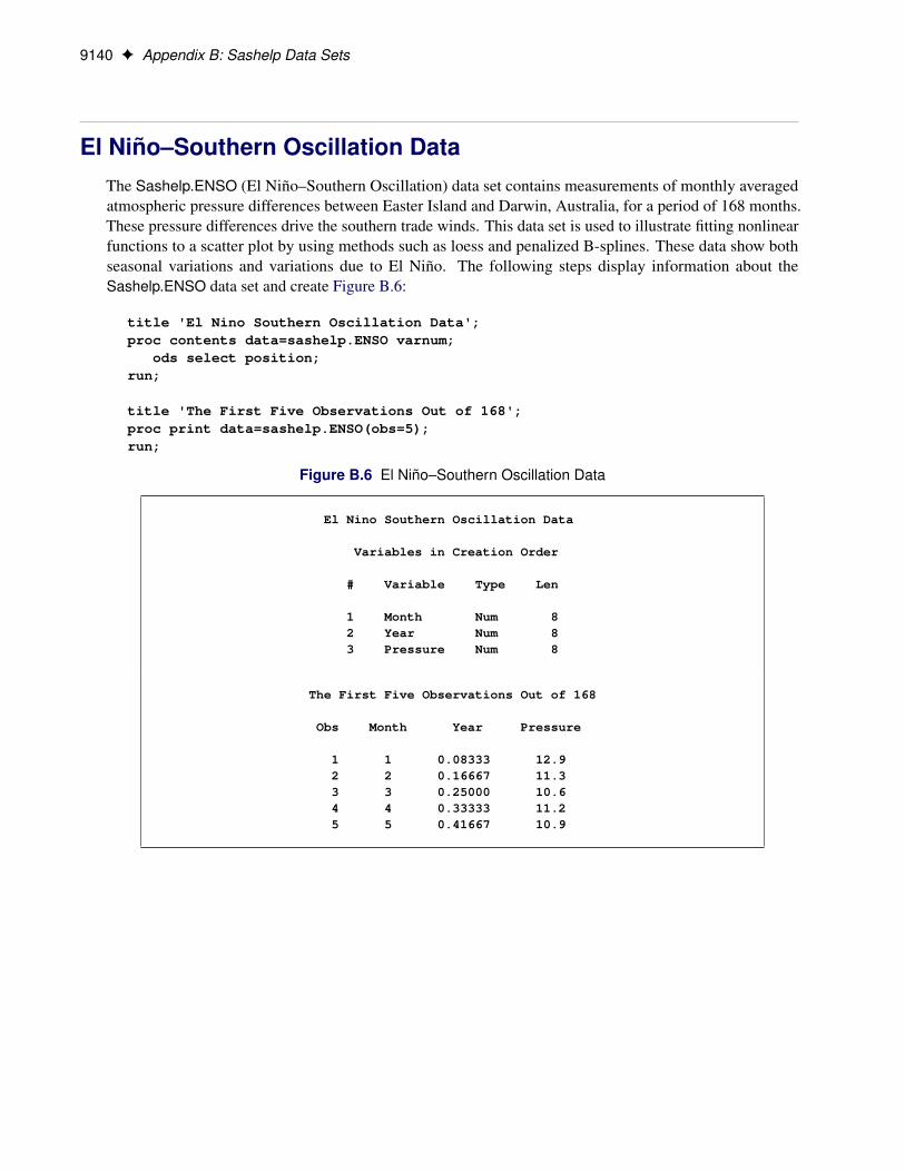
El Niño–Southern Oscillation DataThe Sashelp.ENSO (El Niño–Southern Oscillation) data set contains measurements of monthly averagedatmospheric pressure differences between Easter Island and Darwin, Australia, for a period of 168 months.These pressure differences drive the southern trade winds. This data set is used to illustrate fitting nonlinearfunctions to a scatter plot by using methods such as loess and penalized B-splines. These data show bothseasonal variations and variations due to El Niño. The following steps display information about theSashelp.ENSO data set and create Figure B.6:
title 'El Nino Southern Oscillation Data';proc contents data=sashelp.ENSO varnum;
ods select position;run;
title 'The First Five Observations Out of 168';proc print data=sashelp.ENSO(obs=5);run;
Figure B.6 El Niño–Southern Oscillation Data
El Nino Southern Oscillation Data
Variables in Creation Order
# Variable Type Len
1 Month Num 82 Year Num 83 Pressure Num 8
The First Five Observations Out of 168
Obs Month Year Pressure
1 1 0.08333 12.92 2 0.16667 11.33 3 0.25000 10.64 4 0.33333 11.25 5 0.41667 10.9

Finland’s Lake Laengelmaevesi Fish Catch Data F 9141
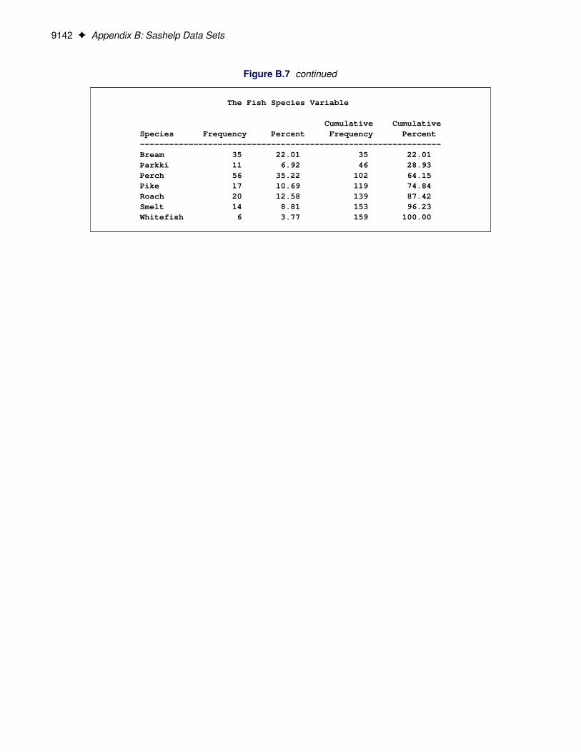
Finland’s Lake Laengelmaevesi Fish Catch DataThe Sashelp.Fish catch data set contains measurements of 159 fish that were caught in Finland’s LakeLaengelmaevesi; it is used to illustrate discriminant analysis. For each of the seven species (bream, roach,whitefish, parkki, perch, pike, and smelt), the weight, length, height, and width of each fish are tallied. Threedifferent length measurements are recorded: from the nose of the fish to the beginning of its tail, from thenose to the notch of its tail, and from the nose to the end of its tail. The height and width are recorded aspercentages of the third length variable. The following steps display information about the Sashelp.Fish dataset and create Figure B.7:
title 'Finland''s Lake Laengelmaevesi Fish Catch Data';proc contents data=sashelp.Fish varnum;
ods select position;run;
title 'The First Five Observations Out of 159';proc print data=sashelp.Fish(obs=5);run;
title 'The Fish Species Variable';proc freq data=sashelp.Fish;
tables species;run;
Figure B.7 Finland’s Lake Laengelmaevesi Fish Catch Data
Finland's Lake Laengelmaevesi Fish Catch Data
Variables in Creation Order
# Variable Type Len
1 Species Char 92 Weight Num 83 Length1 Num 84 Length2 Num 85 Length3 Num 86 Height Num 87 Width Num 8
The First Five Observations Out of 159
Obs Species Weight Length1 Length2 Length3 Height Width
1 Bream 242 23.2 25.4 30.0 11.5200 4.02002 Bream 290 24.0 26.3 31.2 12.4800 4.30563 Bream 340 23.9 26.5 31.1 12.3778 4.69614 Bream 363 26.3 29.0 33.5 12.7300 4.45555 Bream 430 26.5 29.0 34.0 12.4440 5.1340
9142 F Appendix B: Sashelp Data Sets
Figure B.7 continued
The Fish Species Variable
Cumulative CumulativeSpecies Frequency Percent Frequency Percent--------------------------------------------------------------Bream 35 22.01 35 22.01Parkki 11 6.92 46 28.93Perch 56 35.22 102 64.15Pike 17 10.69 119 74.84Roach 20 12.58 139 87.42Smelt 14 8.81 153 96.23Whitefish 6 3.77 159 100.00
Exhaust Emissions Data F 9143
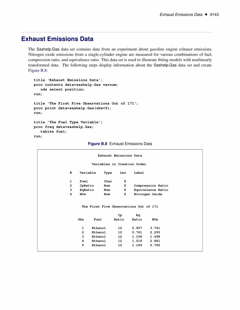
Exhaust Emissions DataThe Sashelp.Gas data set contains data from an experiment about gasoline engine exhaust emissions.Nitrogen oxide emissions from a single-cylinder engine are measured for various combinations of fuel,compression ratio, and equivalence ratio. This data set is used to illustrate fitting models with nonlinearlytransformed data. The following steps display information about the Sashelp.Gas data set and createFigure B.8:
title 'Exhaust Emissions Data';proc contents data=sashelp.Gas varnum;
ods select position;run;
title 'The First Five Observations Out of 171';proc print data=sashelp.Gas(obs=5);run;
title 'The Fuel Type Variable';proc freq data=sashelp.Gas;
tables fuel;run;
Figure B.8 Exhaust Emissions Data
Exhaust Emissions Data
Variables in Creation Order
# Variable Type Len Label
1 Fuel Char 82 CpRatio Num 8 Compression Ratio3 EqRatio Num 8 Equivalence Ratio4 NOx Num 8 Nitrogen Oxide
The First Five Observations Out of 171
Cp EqObs Fuel Ratio Ratio NOx
1 Ethanol 12 0.907 3.7412 Ethanol 12 0.761 2.2953 Ethanol 12 1.108 1.4984 Ethanol 12 1.016 2.8815 Ethanol 12 1.189 0.760
9144 F Appendix B: Sashelp Data Sets
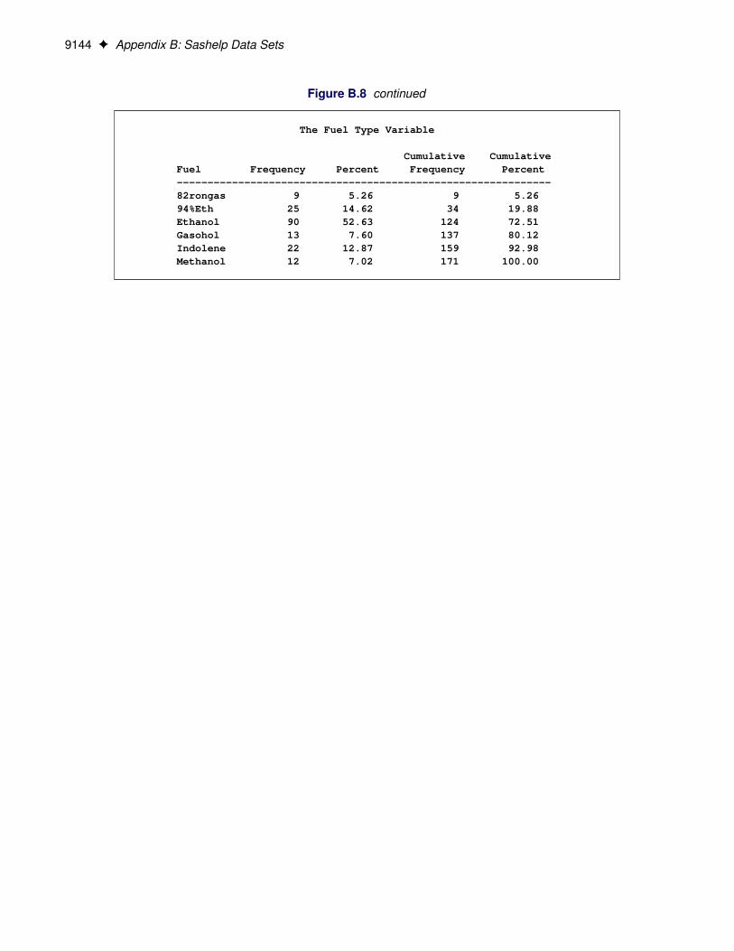
Figure B.8 continued
The Fuel Type Variable
Cumulative CumulativeFuel Frequency Percent Frequency Percent-------------------------------------------------------------82rongas 9 5.26 9 5.2694%Eth 25 14.62 34 19.88Ethanol 90 52.63 124 72.51Gasohol 13 7.60 137 80.12Indolene 22 12.87 159 92.98Methanol 12 7.02 171 100.00
Fisher (1936) Iris Data F 9145
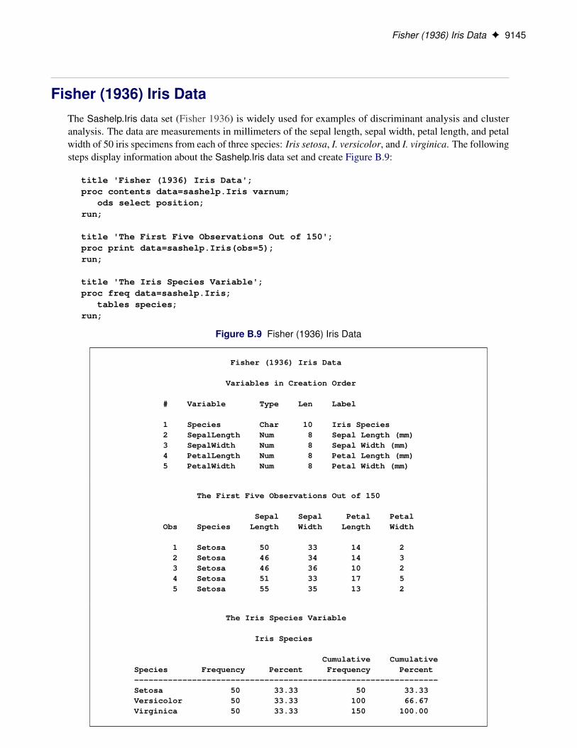
Fisher (1936) Iris DataThe Sashelp.Iris data set (Fisher 1936) is widely used for examples of discriminant analysis and clusteranalysis. The data are measurements in millimeters of the sepal length, sepal width, petal length, and petalwidth of 50 iris specimens from each of three species: Iris setosa, I. versicolor, and I. virginica. The followingsteps display information about the Sashelp.Iris data set and create Figure B.9:
title 'Fisher (1936) Iris Data';proc contents data=sashelp.Iris varnum;
ods select position;run;
title 'The First Five Observations Out of 150';proc print data=sashelp.Iris(obs=5);run;
title 'The Iris Species Variable';proc freq data=sashelp.Iris;
tables species;run;
Figure B.9 Fisher (1936) Iris Data
Fisher (1936) Iris Data
Variables in Creation Order
# Variable Type Len Label
1 Species Char 10 Iris Species2 SepalLength Num 8 Sepal Length (mm)3 SepalWidth Num 8 Sepal Width (mm)4 PetalLength Num 8 Petal Length (mm)5 PetalWidth Num 8 Petal Width (mm)
The First Five Observations Out of 150
Sepal Sepal Petal PetalObs Species Length Width Length Width
1 Setosa 50 33 14 22 Setosa 46 34 14 33 Setosa 46 36 10 24 Setosa 51 33 17 55 Setosa 55 35 13 2
The Iris Species Variable
Iris Species
Cumulative CumulativeSpecies Frequency Percent Frequency Percent---------------------------------------------------------------Setosa 50 33.33 50 33.33Versicolor 50 33.33 100 66.67Virginica 50 33.33 150 100.00
9146 F Appendix B: Sashelp Data Sets
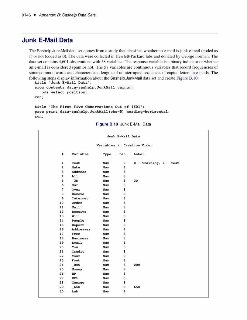
Junk E-Mail DataThe Sashelp.JunkMail data set comes from a study that classifies whether an e-mail is junk e-mail (coded as1) or not (coded as 0). The data were collected in Hewlett-Packard labs and donated by George Forman. Thedata set contains 4,601 observations with 58 variables. The response variable is a binary indicator of whetheran e-mail is considered spam or not. The 57 variables are continuous variables that record frequencies ofsome common words and characters and lengths of uninterrupted sequences of capital letters in e-mails. Thefollowing steps display information about the Sashelp.JunkMail data set and create Figure B.10:
title 'Junk E-Mail Data';proc contents data=sashelp.JunkMail varnum;
ods select position;run;
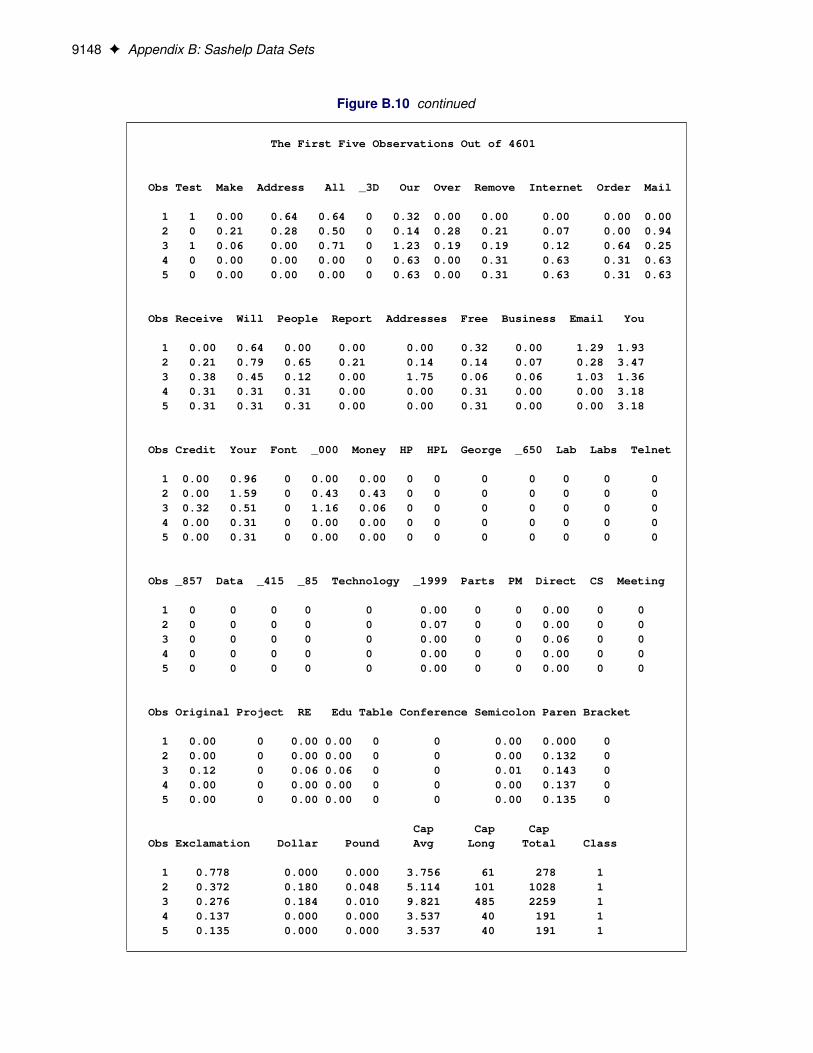
title 'The First Five Observations Out of 4601';proc print data=sashelp.JunkMail(obs=5) heading=horizontal;run;
Figure B.10 Junk E-Mail Data
Junk E-Mail Data
Variables in Creation Order
# Variable Type Len Label
1 Test Num 8 0 - Training, 1 - Test2 Make Num 83 Address Num 84 All Num 85 _3D Num 8 3D6 Our Num 87 Over Num 88 Remove Num 89 Internet Num 8
10 Order Num 811 Mail Num 812 Receive Num 813 Will Num 814 People Num 815 Report Num 816 Addresses Num 817 Free Num 818 Business Num 819 Email Num 820 You Num 821 Credit Num 822 Your Num 823 Font Num 824 _000 Num 8 00025 Money Num 826 HP Num 827 HPL Num 828 George Num 829 _650 Num 8 65030 Lab Num 8
Junk E-Mail Data F 9147
Figure B.10 continued
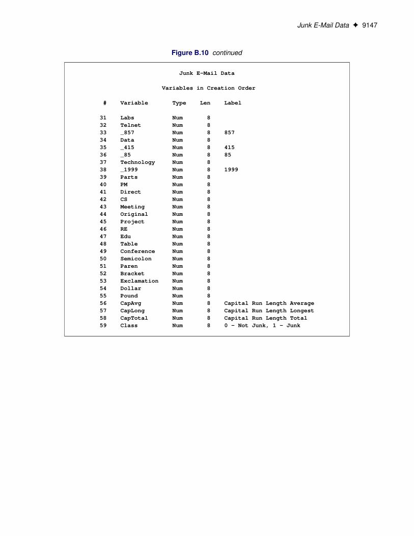
Junk E-Mail Data
Variables in Creation Order
# Variable Type Len Label
31 Labs Num 832 Telnet Num 833 _857 Num 8 85734 Data Num 835 _415 Num 8 41536 _85 Num 8 8537 Technology Num 838 _1999 Num 8 199939 Parts Num 840 PM Num 841 Direct Num 842 CS Num 843 Meeting Num 844 Original Num 845 Project Num 846 RE Num 847 Edu Num 848 Table Num 849 Conference Num 850 Semicolon Num 851 Paren Num 852 Bracket Num 853 Exclamation Num 854 Dollar Num 855 Pound Num 856 CapAvg Num 8 Capital Run Length Average57 CapLong Num 8 Capital Run Length Longest58 CapTotal Num 8 Capital Run Length Total59 Class Num 8 0 - Not Junk, 1 - Junk
9148 F Appendix B: Sashelp Data Sets
Figure B.10 continued
The First Five Observations Out of 4601
Obs Test Make Address All _3D Our Over Remove Internet Order Mail
1 1 0.00 0.64 0.64 0 0.32 0.00 0.00 0.00 0.00 0.002 0 0.21 0.28 0.50 0 0.14 0.28 0.21 0.07 0.00 0.943 1 0.06 0.00 0.71 0 1.23 0.19 0.19 0.12 0.64 0.254 0 0.00 0.00 0.00 0 0.63 0.00 0.31 0.63 0.31 0.635 0 0.00 0.00 0.00 0 0.63 0.00 0.31 0.63 0.31 0.63
Obs Receive Will People Report Addresses Free Business Email You
1 0.00 0.64 0.00 0.00 0.00 0.32 0.00 1.29 1.932 0.21 0.79 0.65 0.21 0.14 0.14 0.07 0.28 3.473 0.38 0.45 0.12 0.00 1.75 0.06 0.06 1.03 1.364 0.31 0.31 0.31 0.00 0.00 0.31 0.00 0.00 3.185 0.31 0.31 0.31 0.00 0.00 0.31 0.00 0.00 3.18
Obs Credit Your Font _000 Money HP HPL George _650 Lab Labs Telnet
1 0.00 0.96 0 0.00 0.00 0 0 0 0 0 0 02 0.00 1.59 0 0.43 0.43 0 0 0 0 0 0 03 0.32 0.51 0 1.16 0.06 0 0 0 0 0 0 04 0.00 0.31 0 0.00 0.00 0 0 0 0 0 0 05 0.00 0.31 0 0.00 0.00 0 0 0 0 0 0 0
Obs _857 Data _415 _85 Technology _1999 Parts PM Direct CS Meeting
1 0 0 0 0 0 0.00 0 0 0.00 0 02 0 0 0 0 0 0.07 0 0 0.00 0 03 0 0 0 0 0 0.00 0 0 0.06 0 04 0 0 0 0 0 0.00 0 0 0.00 0 05 0 0 0 0 0 0.00 0 0 0.00 0 0
Obs Original Project RE Edu Table Conference Semicolon Paren Bracket
1 0.00 0 0.00 0.00 0 0 0.00 0.000 02 0.00 0 0.00 0.00 0 0 0.00 0.132 03 0.12 0 0.06 0.06 0 0 0.01 0.143 04 0.00 0 0.00 0.00 0 0 0.00 0.137 05 0.00 0 0.00 0.00 0 0 0.00 0.135 0
Cap Cap CapObs Exclamation Dollar Pound Avg Long Total Class
1 0.778 0.000 0.000 3.756 61 278 12 0.372 0.180 0.048 5.114 101 1028 13 0.276 0.184 0.010 9.821 485 2259 14 0.137 0.000 0.000 3.537 40 191 15 0.135 0.000 0.000 3.537 40 191 1
Leukemia Data Sets F 9149
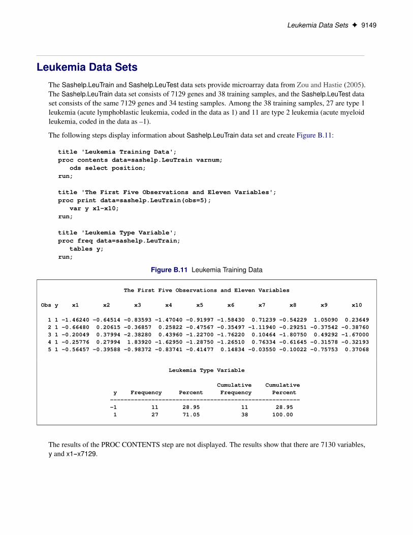
Leukemia Data SetsThe Sashelp.LeuTrain and Sashelp.LeuTest data sets provide microarray data from Zou and Hastie (2005).The Sashelp.LeuTrain data set consists of 7129 genes and 38 training samples, and the Sashelp.LeuTest dataset consists of the same 7129 genes and 34 testing samples. Among the 38 training samples, 27 are type 1leukemia (acute lymphoblastic leukemia, coded in the data as 1) and 11 are type 2 leukemia (acute myeloidleukemia, coded in the data as –1).
The following steps display information about Sashelp.LeuTrain data set and create Figure B.11:
title 'Leukemia Training Data';proc contents data=sashelp.LeuTrain varnum;
ods select position;run;
title 'The First Five Observations and Eleven Variables';proc print data=sashelp.LeuTrain(obs=5);
var y x1-x10;run;
title 'Leukemia Type Variable';proc freq data=sashelp.LeuTrain;
tables y;run;
Figure B.11 Leukemia Training Data
The First Five Observations and Eleven Variables
Obs y x1 x2 x3 x4 x5 x6 x7 x8 x9 x10
1 1 -1.46240 -0.64514 -0.83593 -1.47040 -0.91997 -1.58430 0.71239 -0.54229 1.05090 0.236492 1 -0.66480 0.20615 -0.36857 0.25822 -0.47567 -0.35497 -1.11940 -0.29251 -0.37542 -0.387603 1 -0.20049 0.37994 -2.38280 0.43960 -1.22700 -1.76220 0.10464 -1.80750 0.49292 -1.670004 1 -0.25776 0.27994 1.83920 -1.62950 -1.28750 -1.26510 0.76334 -0.61645 -0.31578 -0.321935 1 -0.56457 -0.39588 -0.98372 -0.83741 -0.41477 0.14834 -0.03550 -0.10022 -0.75753 0.37068
Leukemia Type Variable
Cumulative Cumulativey Frequency Percent Frequency Percent
--------------------------------------------------------1 11 28.95 11 28.951 27 71.05 38 100.00
The results of the PROC CONTENTS step are not displayed. The results show that there are 7130 variables,y and x1-x7129.

9150 F Appendix B: Sashelp Data Sets
The following steps display information about Sashelp.LeuTest data set and create Figure B.12:
title 'Leukemia Test Data';proc contents data=sashelp.LeuTest varnum;
ods select position;run;
title 'The First Five Observations and Eleven Variables';proc print data=sashelp.LeuTest(obs=5);
var y x1-x10;run;
title 'Leukemia Type Variable';proc freq data=sashelp.LeuTest;
tables y;run;
Figure B.12 Leukemia Test Data
The First Five Observations and Eleven Variables
Obs y x1 x2 x3 x4 x5 x6 x7 x8 x9 x10
1 1 -1.38240 0.06288 0.62252 1.61210 0.52179 0.11516 -1.85270 -0.39956 0.88007 -0.865652 1 0.65192 -0.35476 2.29630 1.64980 0.50211 -0.37315 1.76820 -1.74270 1.63080 0.601713 1 0.65409 1.41340 0.22593 -0.06719 0.30015 0.76964 -0.26212 0.94481 -0.51884 -0.609994 1 1.07220 0.01959 0.16875 0.84779 0.24533 0.79682 0.41442 0.35122 -0.70177 1.854105 1 2.12480 1.66370 -0.35986 1.15850 0.89379 0.56310 -0.92476 0.56790 -0.56039 -2.12400
Leukemia Type Variable
Cumulative Cumulativey Frequency Percent Frequency Percent
--------------------------------------------------------1 14 41.18 14 41.181 20 58.82 34 100.00
The results of the PROC CONTENTS step are not displayed. The results show that there are 7130 variables,y and x1-x7129.

Margarine Data F 9151
Margarine DataThe Sashelp.Margarin data set is a scanner panel data set that lists purchases of margarine. There are313 households and a total of 3,405 purchases. The variable HouseID represents the household ID; eachhousehold made at least five purchases, which are defined by the choice set variable Set. The variableChoice represents the choice that households made among the six margarine brands for each purchase orchoice set. The variable Brand has the value ‘PPK’ for Parkay stick, ‘PBB’ for Blue Bonnet stick, ‘PFL’ forFleischmann’s stick, ‘PHse’ for the house brand stick, ‘PGen’ for the generic stick, and ‘PSS’ for Shedd’sSpread tub. The variable LogPrice is the logarithm of the product price. The variables LogInc and FamSizeprovide information about household income and family size, respectively. The following steps displayinformation about the Sashelp.Margarin data set and create Figure B.13:
title 'Margarine Data';proc contents data=sashelp.Margarin varnum;
ods select position;run;
title 'The First Five Observations Out of 20,430';proc print data=sashelp.Margarin(obs=5);run;
Figure B.13 Margarine Data
Margarine Data
Variables in Creation Order
# Variable Type Len
1 HouseID Num 82 Set Num 83 Choice Num 84 Brand Char 85 LogPrice Num 86 LogInc Num 87 FamSize Num 8
The First Five Observations Out of 20,430
FamObs HouseID Set Choice Brand LogPrice LogInc Size
1 2100016 1 1 PPk -0.41552 3.48124 22 2100016 1 0 PBB -0.40048 3.48124 23 2100016 1 0 PFl 0.08618 3.48124 24 2100016 1 0 PHse -0.56212 3.48124 25 2100016 1 0 PGen -1.02165 3.48124 2
9152 F Appendix B: Sashelp Data Sets
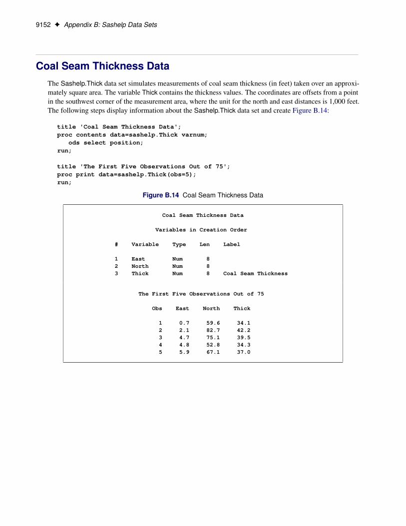
Coal Seam Thickness DataThe Sashelp.Thick data set simulates measurements of coal seam thickness (in feet) taken over an approxi-mately square area. The variable Thick contains the thickness values. The coordinates are offsets from a pointin the southwest corner of the measurement area, where the unit for the north and east distances is 1,000 feet.The following steps display information about the Sashelp.Thick data set and create Figure B.14:
title 'Coal Seam Thickness Data';proc contents data=sashelp.Thick varnum;
ods select position;run;
title 'The First Five Observations Out of 75';proc print data=sashelp.Thick(obs=5);run;
Figure B.14 Coal Seam Thickness Data
Coal Seam Thickness Data
Variables in Creation Order
# Variable Type Len Label
1 East Num 82 North Num 83 Thick Num 8 Coal Seam Thickness
The First Five Observations Out of 75
Obs East North Thick
1 0.7 59.6 34.12 2.1 82.7 42.23 4.7 75.1 39.54 4.8 52.8 34.35 5.9 67.1 37.0
Flying Mileages between Five US Cities Data F 9153
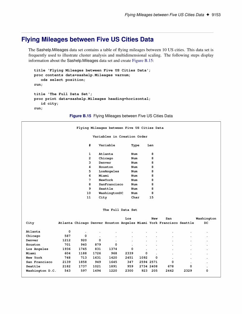
Flying Mileages between Five US Cities DataThe Sashelp.Mileages data set contains a table of flying mileages between 10 US cities. This data set isfrequently used to illustrate cluster analysis and multidimensional scaling. The following steps displayinformation about the Sashelp.Mileages data set and create Figure B.15:
title 'Flying Mileages between Five US Cities Data';proc contents data=sashelp.Mileages varnum;
ods select position;run;
title 'The Full Data Set';proc print data=sashelp.Mileages heading=horizontal;
id city;run;
Figure B.15 Flying Mileages between Five US Cities Data
Flying Mileages between Five US Cities Data
Variables in Creation Order
# Variable Type Len
1 Atlanta Num 82 Chicago Num 83 Denver Num 84 Houston Num 85 LosAngeles Num 86 Miami Num 87 NewYork Num 88 SanFrancisco Num 89 Seattle Num 8
10 WashingtonDC Num 811 City Char 15
The Full Data Set
Los New San WashingtonCity Atlanta Chicago Denver Houston Angeles Miami York Francisco Seattle DC
Atlanta 0 . . . . . . . . .Chicago 587 0 . . . . . . . .Denver 1212 920 0 . . . . . . .Houston 701 940 879 0 . . . . . .Los Angeles 1936 1745 831 1374 0 . . . . .Miami 604 1188 1726 968 2339 0 . . . .New York 748 713 1631 1420 2451 1092 0 . . .San Francisco 2139 1858 949 1645 347 2594 2571 0 . .Seattle 2182 1737 1021 1891 959 2734 2408 678 0 .Washington D.C. 543 597 1494 1220 2300 923 205 2442 2329 0
9154 F Appendix B: Sashelp Data Sets
References
Fisher, R. A. (1936), “The Use of Multiple Measurements in Taxonomic Problems,” Annals of Eugenics, 7,179–188.
Zou, H. and Hastie, T. (2005), “Regularization and Variable Selection via the Elastic Net,” Journal of theRoyal Statistical Society, Series B, 67, 301–320.