Sarang Sanjay S
170
OHMIC HEATING FOR THERMAL PROCESSING OF LOW-ACID FOODS CONTAINING SOLID PARTICULATES DISSERTATION Presented in Partial Fulfillment of the Requirements for the Degree Doctor of Philosophy in the Graduate School of The Ohio State University By Sanjay S. Sarang, M.S. * * * * * The Ohio State University 2007 Dissertation Committee: Professor Sudhir Sastry, Adviser Professor Ahmed Yousef Professor Harold Keener Professor V. M. Balasubramaniam Approved by Adviser Graduate Program in Food, Agricultural and Biological Engineering
-
Upload
aabid-hussain -
Category
Documents
-
view
133 -
download
0
Transcript of Sarang Sanjay S
5/9/2018 Sarang Sanjay S - slidepdf.com
http://slidepdf.com/reader/full/sarang-sanjay-s 1/170
OHMIC HEATING FOR THERMAL PROCESSING OF LOW-ACID
FOODS CONTAINING SOLID PARTICULATES
DISSERTATION
Presented in Partial Fulfillment of the Requirements for
the Degree Doctor of Philosophy in the GraduateSchool of The Ohio State University
By
Sanjay S. Sarang, M.S.
* * * * *
The Ohio State University2007
Dissertation Committee:
Professor Sudhir Sastry, Adviser
Professor Ahmed Yousef Professor Harold Keener
Professor V. M. Balasubramaniam
Approved by
Adviser
Graduate Program in Food, Agricultural
and Biological Engineering

5/9/2018 Sarang Sanjay S - slidepdf.com
http://slidepdf.com/reader/full/sarang-sanjay-s 2/170
5/9/2018 Sarang Sanjay S - slidepdf.com
http://slidepdf.com/reader/full/sarang-sanjay-s 3/170
ii
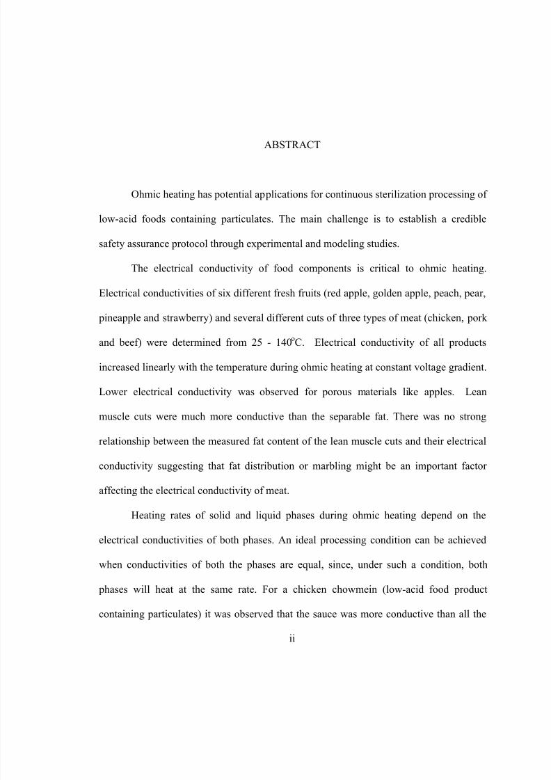
ABSTRACT
Ohmic heating has potential applications for continuous sterilization processing of
low-acid foods containing particulates. The main challenge is to establish a credible
safety assurance protocol through experimental and modeling studies.
The electrical conductivity of food components is critical to ohmic heating.
Electrical conductivities of six different fresh fruits (red apple, golden apple, peach, pear,
pineapple and strawberry) and several different cuts of three types of meat (chicken, pork
and beef) were determined from 25 - 140oC. Electrical conductivity of all products
increased linearly with the temperature during ohmic heating at constant voltage gradient.
Lower electrical conductivity was observed for porous materials like apples. Lean
muscle cuts were much more conductive than the separable fat. There was no strong
relationship between the measured fat content of the lean muscle cuts and their electrical
conductivity suggesting that fat distribution or marbling might be an important factor
affecting the electrical conductivity of meat.
Heating rates of solid and liquid phases during ohmic heating depend on the
electrical conductivities of both phases. An ideal processing condition can be achieved
when conductivities of both the phases are equal, since, under such a condition, both
phases will heat at the same rate. For a chicken chowmein (low-acid food product
containing particulates) it was observed that the sauce was more conductive than all the
5/9/2018 Sarang Sanjay S - slidepdf.com
http://slidepdf.com/reader/full/sarang-sanjay-s 4/170
iii
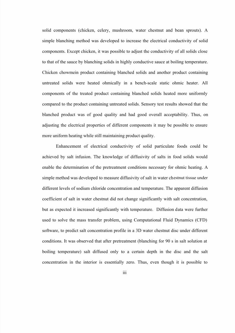
solid components (chicken, celery, mushroom, water chestnut and bean sprouts). A
simple blanching method was developed to increase the electrical conductivity of solid
components. Except chicken, it was possible to adjust the conductivity of all solids close
to that of the sauce by blanching solids in highly conductive sauce at boiling temperature.
Chicken chowmein product containing blanched solids and another product containing
untreated solids were heated ohmically in a bench-scale static ohmic heater. All
components of the treated product containing blanched solids heated more uniformly
compared to the product containing untreated solids. Sensory test results showed that the
blanched product was of good quality and had good overall acceptability. Thus, on
adjusting the electrical properties of different components it may be possible to ensure
more uniform heating while still maintaining product quality.
Enhancement of electrical conductivity of solid particulate foods could be
achieved by salt infusion. The knowledge of diffusivity of salts in food solids would
enable the determination of the pretreatment conditions necessary for ohmic heating. A
simple method was developed to measure diffusivity of salt in water chestnut tissue under
different levels of sodium chloride concentration and temperature. The apparent diffusion
coefficient of salt in water chestnut did not change significantly with salt concentration,
but as expected it increased significantly with temperature. Diffusion data were further
used to solve the mass transfer problem, using Computational Fluid Dynamics (CFD)
software, to predict salt concentration profile in a 3D water chestnut disc under different
conditions. It was observed that after pretreatment (blanching for 90 s in salt solution at
boiling temperature) salt diffused only to a certain depth in the disc and the salt
concentration in the interior is essentially zero. Thus, even though it is possible to
5/9/2018 Sarang Sanjay S - slidepdf.com
http://slidepdf.com/reader/full/sarang-sanjay-s 5/170
iv
increase the overall ionic content and electrical conductivity of solids by blanching in
highly conductive sauce, conductivity may not be uniform within the solids. However,
even this limited diffusion is useful in improving solids heating.
Measurement of residence time distribution (RTD) is needed for determination of
the fastest-moving particle, to be used for designing and biologically validating
processes. Radio Frequency Identification (RFID) was used to measure residence time
distribution (RTD) of particles in the ohmic heater in a continuous sterilization process.
The residence times and the residence time distribution of a model food particle system
(potato in starch solution) were investigated in the ohmic heater. The effect of six levels
of solid concentration and three levels of rotational speed of the agitators on the RTD
were studied. Mean particle residence time increased with the rotational speed of
agitators in the ohmic heaters. Mean particle velocities were greater than the mean
product velocity. The velocity of the fastest particle was 1.62 times the mean product
velocity which is less than that associated with Newtonian fluid in tubular flow.

5/9/2018 Sarang Sanjay S - slidepdf.com
http://slidepdf.com/reader/full/sarang-sanjay-s 6/170
v
Dedicated to my parents
5/9/2018 Sarang Sanjay S - slidepdf.com
http://slidepdf.com/reader/full/sarang-sanjay-s 7/170
vi
ACKNOWLEDGMENTS
I would like to express my sincere appreciation and gratitude to my advisor, Dr.
Sudhir Sastry for his guidance throughout with my dissertation. Special thanks to him for
supporting me during toughest time in my life. I also extend my gratitude to Drs.
BalaBalsubramanium, Ahmed Yousef and Harold Keener, dissertation committee, for
their valuable comments and remarks. I acknowledge the technical assistance by Brian
Heskitt.
I thank my sisters for their unwavering support. They are my strong four pillars.
I thank Dr. Knipe, Dr. Soojin Jun and Ankan Kumar for the technical help. I am
grateful to all the members in Dr. Sastry’s research team for their assistance, helpful
discussions, and above all their kindness and friendship. I thank my friends in Columbus
who made my stay at OSU a memorable one. Thank you guys for being there for me
during my tough times- I love you all for that. I would also like to acknowledge my
friends from school, college and UDCT for their friendship and support.
5/9/2018 Sarang Sanjay S - slidepdf.com
http://slidepdf.com/reader/full/sarang-sanjay-s 8/170
vii
VITA
October 12, 1978 ……………….. Born – Mumbai, India
2004……………………………... M.S. Chemical Engineering, University of Cincinnati, Cincinnati, OH.
2004 – present …………………...Graduate Research Associate, The Ohio StateUniversity
PUBLICATIONS
Research Publications
1. Sanjay Sarang & Sudhir K. Sastry (2007) Diffusion and equilibrium
distribution coefficients of salt within vegetable tissue: effects of salt concentration
and temperature. Journal of Food Engineering, 82, 377-382.
2. Sanjay Sarang, S.K. Sastry, J. Gaines, T.C.S. Yang, & P. Dunne (2007) Product
formulation for ohmic heating: blanching as a pretreatment method to improve
uniformity in heating of solid-liquid food mixtures. Journal of Food Science, E . 72
(5), 227-234.
FIELDS OF STUDY
Major Field: Food, Agricultural and Biological Engineering
5/9/2018 Sarang Sanjay S - slidepdf.com
http://slidepdf.com/reader/full/sarang-sanjay-s 9/170
viii
TABLE OF CONTENTS
Page
Abstract …………………………………………………………………………………...ii
Dedication ………………………………………………………………………………...v
Acknowledgments …………………………………………………………………….....vi
Vita ……………………………………………………………………………………...vii
List of Tables …………………………………………………………………………....xii
List of Figures …………………………………………………………………………..xiv
Chapters:
1. Introduction …………………………………………………………………………1
1.1 Nomenclature ……………………………………………………………..6
1.2 References ………………………………………………………………...6
2. Electrical conductivity of fruits and meats during ohmic heating ………………...11
2.1 Abstract ………………………………………………………………….11
2.2 Introduction ……………………………………………………………...12
2.3 Materials and methods …………………………………………………..13
2.3.1 Electrical conductivity ………………………………………………...14
2.3.1.1 Experimental device ………………………………………………....14
2.3.1.2 Methodology ………………………………………………………...14
2.3.1.3 Analysis ……………………………………………………………...15
5/9/2018 Sarang Sanjay S - slidepdf.com
http://slidepdf.com/reader/full/sarang-sanjay-s 10/170
ix
2.3.1.4 Error estimation ……………………………………………………..15
2.3.2 Fat analysis of meat …………………………………………………...16
2.4 Results and discussion …………………………………………………..16
2.5 Conclusions ……………………………………………………………...20
2.6 Nomenclature ……………………………………………………………21
2.7 References ……………………………………………………………….21
2.8 Figures …………………………………………………………………...25
2.9 Tables …………………………………………………………………...32
3. Blanching as a pretreatment method to improve uniformity in heating of
solid-liquid food mixtures ………………………………………………..………..39
3.1
Abstract …………………………………………………………...……..393.2 Introduction ……………………………………………………………...40
3.3 Materials and methods …………………………………………………..43
3.3.1 Determination of electrical conductivity ……………………………...44
3.3.2 Blanching ……………………………………………………………...44
3.3.3 Ohmic heating and determination of heating rates ……………………45
3.3.4 Sensory evaluation …………………………………………………….46
3.4 Results and discussion …………………………………………………..47
3.5 Conclusions ……………………………………………………………...49
3.6 Nomenclature ……………………………………………………………50
3.7 References ……………………………………………………………….50
3.8 Figures …………………………………………………………………...52
3.9 Tables ……………………………………………………………………62
4. Salt diffusion into vegetable tissue as a pretreatment for ohmic heating …………65
4.1 Abstract ………………………………………………………………….65
4.2 Introduction ……………………………………………………………...66
4.3 Materials and methods …………………………………………………..68
4.3.1 Mathematical model …………………………………………………...68
4.3.2 Experimental procedure ……………………………………………….69
5/9/2018 Sarang Sanjay S - slidepdf.com
http://slidepdf.com/reader/full/sarang-sanjay-s 11/170
x
4.3.2.1 Determination of equilibrium distribution coefficient (K) ………….70
4.3.2.2 Determination of apparent diffusion coefficient (Ds) ……………….70
4.3.3 Statistical analysis ……………………………………………………..71
4.3.4 Computational simulation …………………………………………….71
4.3.4.1 Blanching ……………………………………………………………71
4.3.4.2 Blanching followed by ohmic heating………………………………72
4.3.4.3 Ohmic heating of unblanched solid …………………………………74
4.4 Results and discussion …………………………………………………..75
4.4.1 Equilibrium distribution coefficient …………………………………...75
4.4.2 Apparent diffusion coefficient ………………………………………...76
4.4.3 Simulation ……………………………………………………………..78
4.4.3.1 Blanching ……………………………………………………………78
4.4.3.2 Ohmic heating of blanched solid ……………………………………79
4.5 Conclusions ……………………………………………………………...79
4.6 Nomenclature ……………………………………………………………80
4.7 References ……………………………………………………………….82
4.8 Figures …………………………………………………………………...85
4.9 Tables …………………………………………………………………..105
5. Residence time distribution (RTD) of particulate foods in a continuous flow
pilot-scale ohmic heater …………………………………………………………107
5.1 Abstract ………………………………………………………………...107
5.2 Introduction …………………………………………………………….108
5.3 Materials and methods …………………………………………………112
5.3.1 Product ……………………………………………………………….112
5.3.2 Analog particles ……………………………………………………...112
5.3.3 Ohmic heating pilot plant facility ……………………………………113
5.3.4 Radio Frequency Identification (RFID) ……………………………...114
5.3.5 Experimental method ………………………………………………...114
5.4 Results and discussion …………………………………………………116
5.5 Conclusions …………………………………………………………….119

5/9/2018 Sarang Sanjay S - slidepdf.com
http://slidepdf.com/reader/full/sarang-sanjay-s 12/170
xi
5.6 References ……………………………………………………………...119
5.7 Figures ………………………………………………………………….123
5.8 Tables …………………………………………………………………..138
6. Conclusions ………………………………………………………………………143
List of references ……………………………………………………………………….145
5/9/2018 Sarang Sanjay S - slidepdf.com
http://slidepdf.com/reader/full/sarang-sanjay-s 13/170
xii
LIST OF TABLES
Table Page
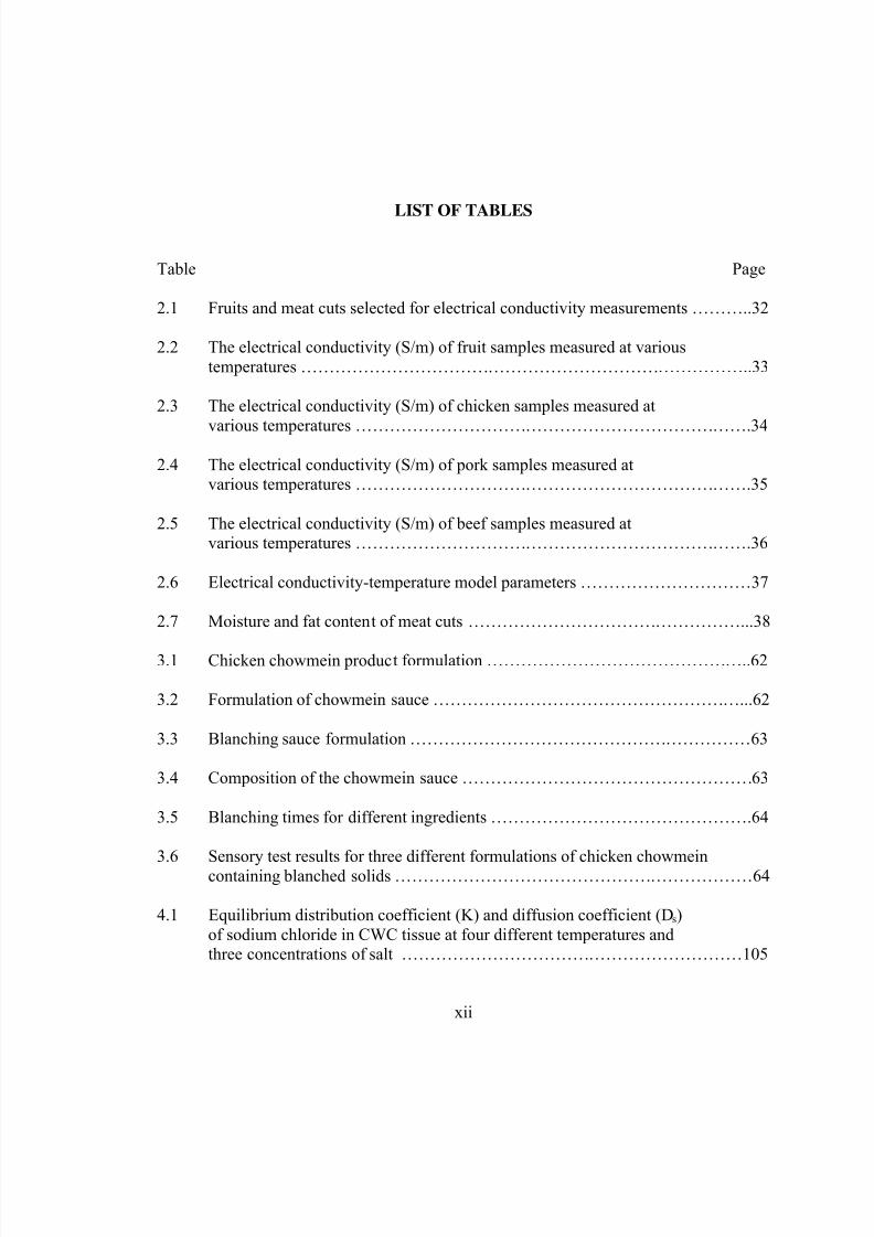
2.1 Fruits and meat cuts selected for electrical conductivity measurements ………..32
2.2 The electrical conductivity (S/m) of fruit samples measured at various
temperatures ……………………………………………………………………..33
2.3 The electrical conductivity (S/m) of chicken samples measured at
various temperatures …………………………………………………………….34
2.4 The electrical conductivity (S/m) of pork samples measured atvarious temperatures …………………………………………………………….35
2.5 The electrical conductivity (S/m) of beef samples measured atvarious temperatures …………………………………………………………….36
2.6 Electrical conductivity-temperature model parameters …………………………37
2.7 Moisture and fat content of meat cuts …………………………………………...38
3.1 Chicken chowmein product formulation ………………………………………..62
3.2 Formulation of chowmein sauce ………………………………………………...62
3.3 Blanching sauce formulation ……………………………………………………63
3.4 Composition of the chowmein sauce ……………………………………………63
3.5 Blanching times for different ingredients ……………………………………….64
3.6
Sensory test results for three different formulations of chicken chowmeincontaining blanched solids ………………………………………………………64
4.1 Equilibrium distribution coefficient (K) and diffusion coefficient (Ds)
of sodium chloride in CWC tissue at four different temperatures and
three concentrations of salt ……………………………………………………105
5/9/2018 Sarang Sanjay S - slidepdf.com
http://slidepdf.com/reader/full/sarang-sanjay-s 14/170
xiii
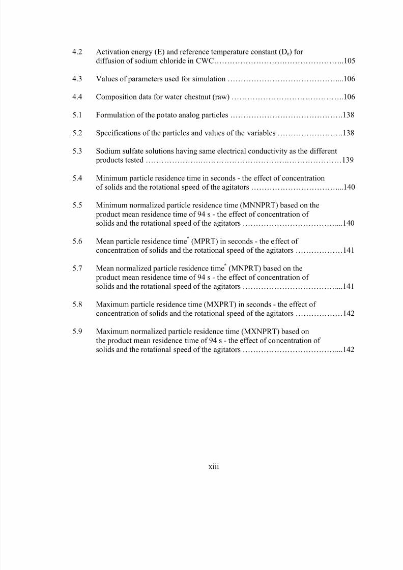
4.2 Activation energy (E) and reference temperature constant (Do) for
diffusion of sodium chloride in CWC…………………………………………..105
4.3 Values of parameters used for simulation ……………………………………...106
4.4
Composition data for water chestnut (raw) …………………………………….106
5.1 Formulation of the potato analog particles …………………………………….138
5.2 Specifications of the particles and values of the variables …………………….138
5.3 Sodium sulfate solutions having same electrical conductivity as the different products tested …………………………………………………………………139
5.4 Minimum particle residence time in seconds - the effect of concentrationof solids and the rotational speed of the agitators ……………………………...140
5.5 Minimum normalized particle residence time (MNNPRT) based on the
product mean residence time of 94 s - the effect of concentration of solids and the rotational speed of the agitators ………………………………...140
5.6 Mean particle residence time*
(MPRT) in seconds - the effect of concentration of solids and the rotational speed of the agitators ………………141
5.7 Mean normalized particle residence time*
(MNPRT) based on the product mean residence time of 94 s - the effect of concentration of
solids and the rotational speed of the agitators ………………………………...141
5.8 Maximum particle residence time (MXPRT) in seconds - the effect of
concentration of solids and the rotational speed of the agitators ………………142
5.9 Maximum normalized particle residence time (MXNPRT) based on
the product mean residence time of 94 s - the effect of concentration of
solids and the rotational speed of the agitators ………………………………...142
5/9/2018 Sarang Sanjay S - slidepdf.com
http://slidepdf.com/reader/full/sarang-sanjay-s 15/170
xiv
LIST OF FIGURES
Figure Page
2.1 Schematic diagram of the experimental setup for electrical conductivity
measurements ……………………………………………………………………25
2.2 Electrical conductivity of fruits (1 std. dev.) ……………………………………26
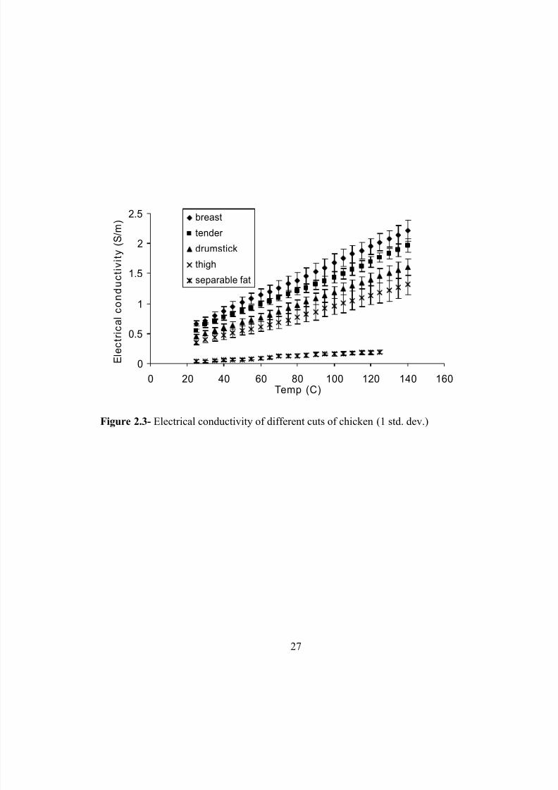
2.3 Electrical conductivity of different cuts of chicken (1 std. dev.) ………………..27
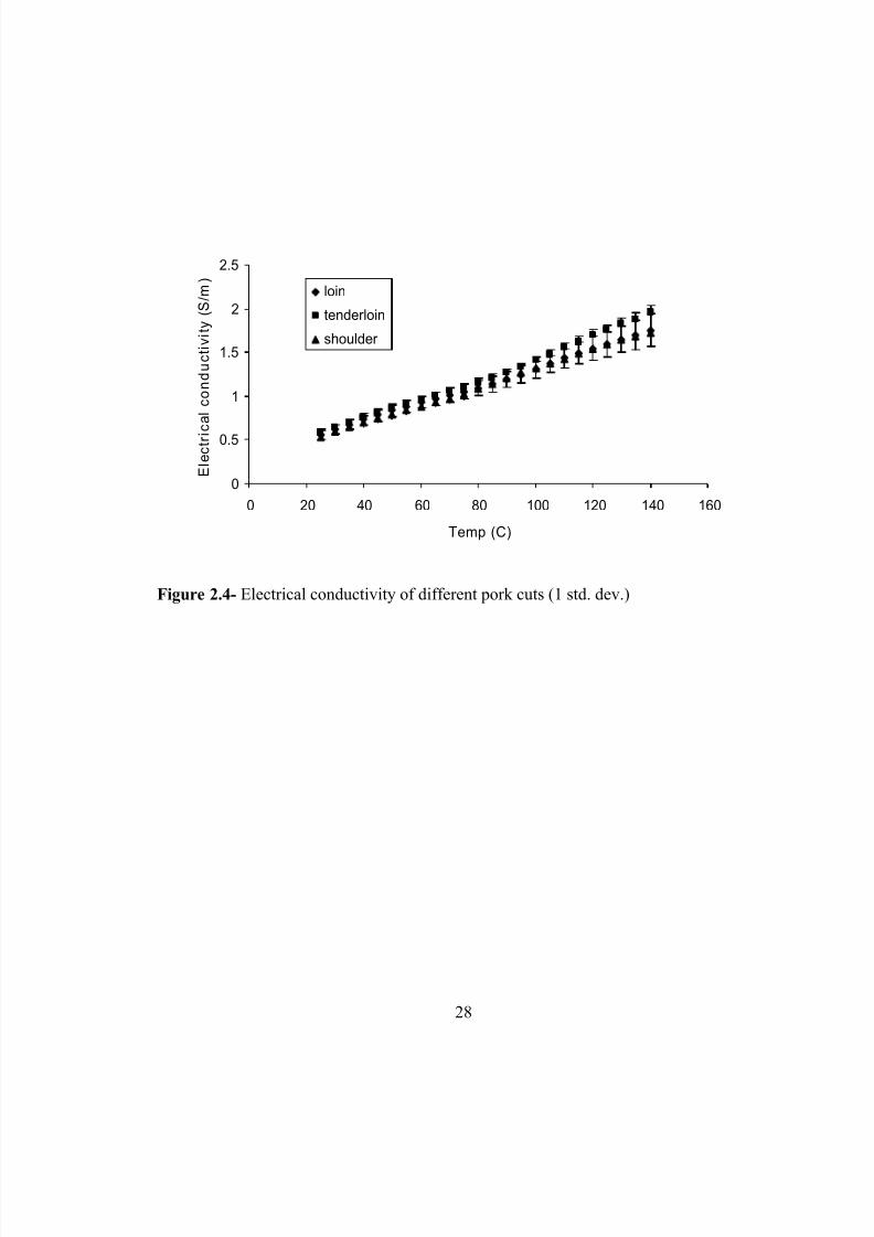
2.4 Electrical conductivity of different pork cuts (1 std. dev.) ……………………...28
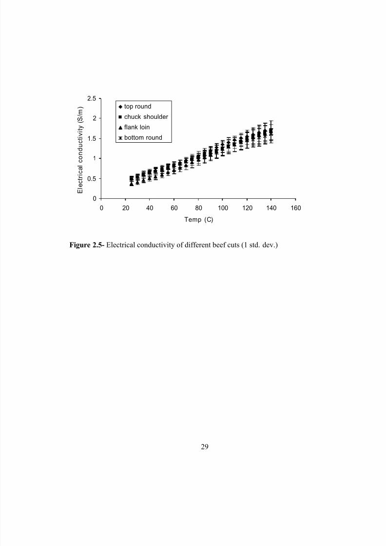
2.5 Electrical conductivity of different beef cuts (1 std. dev.)……………………….29
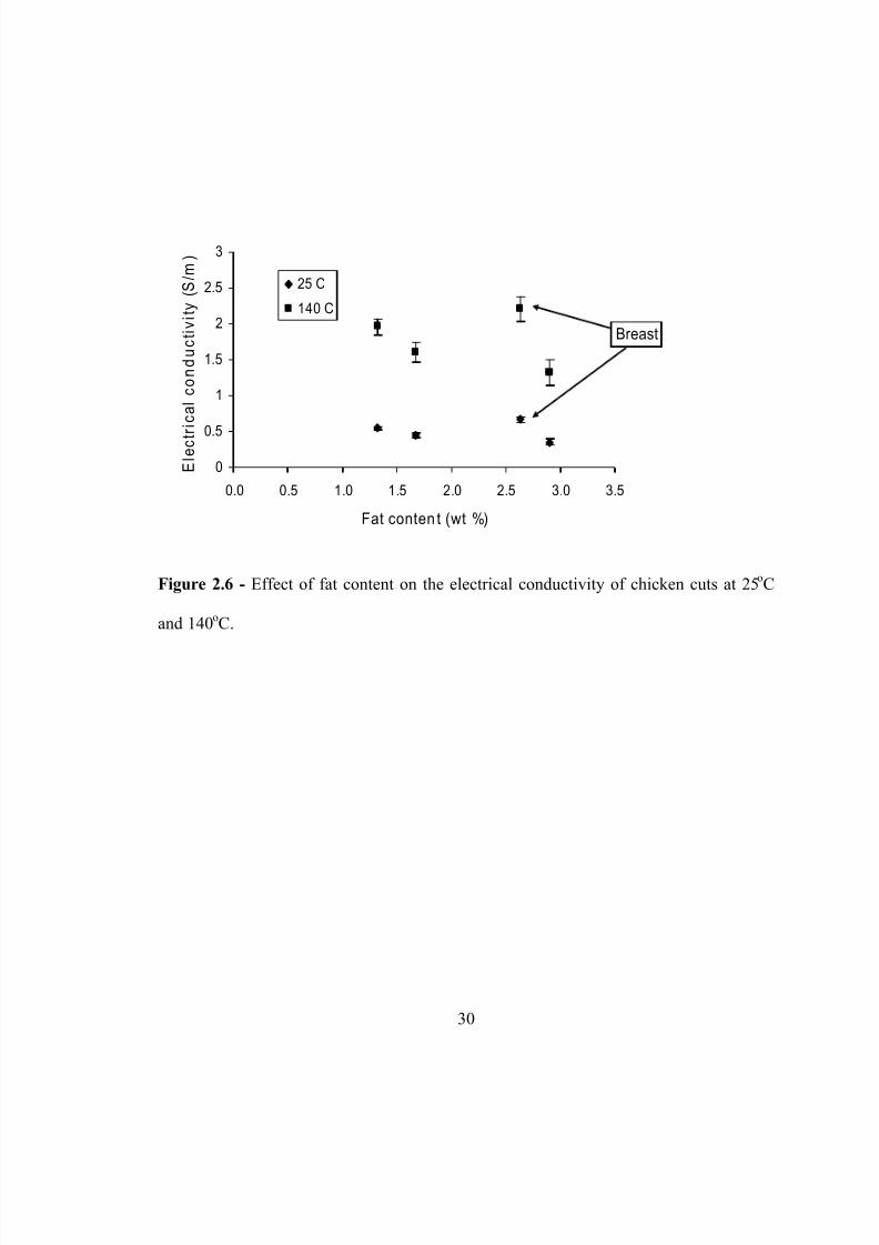
2.6 Effect of fat content on the electrical conductivity of chicken cuts at25
oC and 140
oC ………………………………………………………………….30
2.7 Effect of fat content on the electrical conductivity of lean muscle cutsat 25
oC and 140
oC ……………………………………………………………….31
3.1
Schematic diagram of the experimental setup; ten ohmic heating cellswith relay circuit ………………………………………………………………...52
3.2 Flowchart for pretreatment and subsequent preparation of Chicken
chowmein product ……………………………………………………………….53
3.3 Electrical conductivity variation with temperature of bean sprouts blanched for different times ……………………………………………………..54
3.4 Electrical conductivity variation with temperature of celery blanchedfor different times ……………………………………………………………….55
3.5 Electrical conductivity variation with temperature of water chestnut blanched for different times ……………………………………………………..56
3.6 Electrical conductivity variation with temperature of chicken blanched
for different times ……………………………………………………………….57

5/9/2018 Sarang Sanjay S - slidepdf.com
http://slidepdf.com/reader/full/sarang-sanjay-s 16/170
xv
3.7 Electrical conductivity variation with temperature of mushroom
blanched for different times ……………………………………………………..58
3.8 Electrical conductivity variation with temperature of blanched solid
components, shown together …………………………………………………….59
3.9 Heating rates of different solid components of chicken chowmein with
untreated solids ………………………………………………………………….60
3.10 Heating rates of different solid components of chicken chowmein with
blanched solids …………………………………………………………………..61
4.1 Schematic diagram of the diffusion model ……………………………………...85
4.2 (a) diffusivity cell, and (b) sample holder details ……………………………….86
4.3
Schematic diagram of chestnut disc in box used for simulation studies ………...87
4.4 Electrical conductivity variation with temperature of 5% salt solution …………88
4.5 Electrical conductivity variation with temperature of water chestnut
with 0.015, 2.5 and 5% salt mass fraction ………………………………………89
4.6 Salt concentration change in the solution (C d ) and CWC (C m) for
determination of K (3 replicates at 5% salt concentration and 25oC) …………...90
4.7 Change in salt concentration in the receiver with time for three salt
solutions at (a) 25
o
C; (b) 40
o
C; (c) 60
o
C and (d) 80
o
C ………………………….92
4.8 Change in salt concentration in the receiver with time; (♦) 5% and 25oC,
(▲) 10% and 80oC, and (– ▪ –) theoretical lines …………………………………93
4.9 Comparison of the predicted salt concentration [ M i] for final Ds values
and the salt concentration determined experimentally [C i] ……………………..94
4.10 Concentration and temperature dependence of the apparent diffusion
coefficient ( Ds) of salt in CWC ………………………………………………….95
4.11
Arrhenius plots for apparent diffusion coefficient ( Ds) where T is theabsolute temperature …………………………………………………………….96
4.12 Contours of temperature for water chestnut disc after 10 s of blanching,
shown in y-z plane ………………………………………………………………97
5/9/2018 Sarang Sanjay S - slidepdf.com
http://slidepdf.com/reader/full/sarang-sanjay-s 17/170
xvi
4.13 Contours of temperature for water chestnut disc after 90 s of blanching,
shown in y-z plane ……………………………………………………...……….98
4.14 Contours of salt concentration for water chestnut disc after 90 s of blanching,
shown in y-z plane ………………………………………………………………99
4.15 Contour of salt concentration in water chestnut disc after blanching
Pretreatment of 90 s ……………………………………………………………100
4.16 Contour of temperature within and around the water chestnut disc after
the blanching pretreatment of 90 s ……………………………………………..101
4.17 Contour of electrical conductivity inside the chestnut disc ……………………102
4.18 Contour of temperature within and around the water chestnut disc after
100 s of ohmic heating …………………………………………………………103
4.19 Contour of temperature within and around the unblanched water chestnut discafter100 s of ohmic heating ………………………………………………….104
5.1 Electrical conductivity comparison of blanched potato particles, starchsolution and potato/alginate analog particles (error bars – 1 std. dev.) ………..123
5.2 Diagram of the 54 kW ohmic heating pilot plant facility and positionof RFID readers ………………………………………………………………...124
5.3
Density function E (θ) of the normalized particle residence time in theohmic heater: 30% and 25 rpm …………………………………………..........125
5.4 Density function E (θ) of the normalized particle residence time in the
ohmic heater: 30% and 40 rpm …………………………………………..........126
5.5 Density function E (θ) of the normalized particle residence time in theohmic heater: 30% and 55 rpm …………………………………………..........127
5.6 Density function E (θ) of the normalized particle residence time in theohmic heater: 40% and 25 rpm …………………………………………..........128
5.7 Density function E (θ) of the normalized particle residence time in theohmic heater: 40% and 40 rpm …………………………………………..........129
5.8 Density function E (θ) of the normalized particle residence time in the
ohmic heater: 40% and 55 rpm …………………………………………..........130
5/9/2018 Sarang Sanjay S - slidepdf.com
http://slidepdf.com/reader/full/sarang-sanjay-s 18/170
xvii
5.9 Density function E (θ) of the normalized particle residence time in the
ohmic heater: 50% and 25 rpm …………………………………………..........131
5.10 Density function E (θ) of the normalized particle residence time in the
ohmic heater: 50% and 40 rpm …………………………………………..........132
5.11 Density function E (θ) of the normalized particle residence time in the
ohmic heater: 50% and 55 rpm …………………………………………..........133
5.12 Density function E (θ) of the normalized particle residence time in the
ohmic heater: 60% and 25 rpm …………………………………………..........134
5.13 Density function E (θ) of the normalized particle residence time in the
ohmic heater: 60% and 40 rpm …………………………………………..........135
5.14 Density function E (θ) of the normalized particle residence time in the
ohmic heater: 60% and 55 rpm …………………………………………..........136
5.15 Density function E (θ) of the normalized particle residence time in theohmic heater: 70% and 40 rpm …………………………………………..........137
5/9/2018 Sarang Sanjay S - slidepdf.com
http://slidepdf.com/reader/full/sarang-sanjay-s 19/170
1
CHAPTER 1
INTRODUCTION
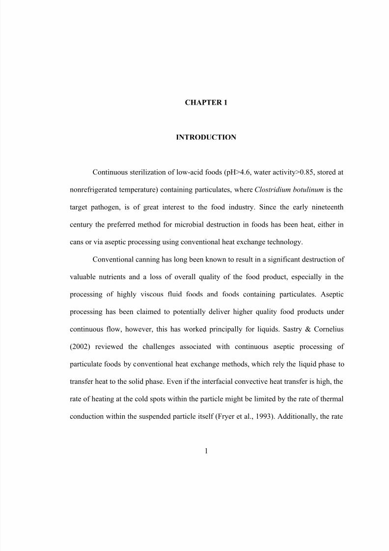
Continuous sterilization of low-acid foods (pH>4.6, water activity>0.85, stored at
nonrefrigerated temperature) containing particulates, where Clostridium botulinum is the
target pathogen, is of great interest to the food industry. Since the early nineteenth
century the preferred method for microbial destruction in foods has been heat, either in
cans or via aseptic processing using conventional heat exchange technology.
Conventional canning has long been known to result in a significant destruction of
valuable nutrients and a loss of overall quality of the food product, especially in the
processing of highly viscous fluid foods and foods containing particulates. Aseptic
processing has been claimed to potentially deliver higher quality food products under
continuous flow, however, this has worked principally for liquids. Sastry & Cornelius
(2002) reviewed the challenges associated with continuous aseptic processing of
particulate foods by conventional heat exchange methods, which rely the liquid phase to
transfer heat to the solid phase. Even if the interfacial convective heat transfer is high, the
rate of heating at the cold spots within the particle might be limited by the rate of thermal
conduction within the suspended particle itself (Fryer et al., 1993). Additionally, the rate
5/9/2018 Sarang Sanjay S - slidepdf.com
http://slidepdf.com/reader/full/sarang-sanjay-s 20/170
of thermal conduction within the solids phase limits the size of the particulates that can
be processed by this conventional technique (de Ruyter & Brunet, 1973).
Ohmic heating offers an attractive alternative because it simultaneously heats both
phases by internal energy generation, and has potential applications for processing such
food products (Palaniappan & Sastry, 2002). For any food product that is commercially
sterilized in the United States, the FDA requires that the sterilization process be filed with
them. A process filing is a document which describes details of the sterilization process
(such as mathematical models, experimental data, microbiological verification data, etc)
which shows that the processor fully understands the sterilization process and is
completely aware of the worst case scenario (Larkin & Spinak, 1996). The identification,
control and validation of all the critical control points required to demonstrate that an
ohmically processed multiphase low acid food product has been rendered commercially
sterile is more difficult than that for conventional methods. A base of knowledge needs to
be developed before ohmic heating can be commercially used. This research project aims
to provide the first steps towards preparation of a model process filing for ohmic heating,
such that, in future any processor interested in ohmic heating can use this model process
filing protocol as a reference for his/her own process.
Ohmic heating involves the application of a cyclical potential to a material,
resulting in heat generation due to ionic motion. The basic relationship for the energy
generation rate is:
2V u ∇= σ & (1.1)
The critical property affecting energy generation is the electrical conductivity (σ) of the
material. Palaniappan & Sastry (1991), and Mitchell & de Alwis (1989) measured
2
5/9/2018 Sarang Sanjay S - slidepdf.com
http://slidepdf.com/reader/full/sarang-sanjay-s 21/170
3
electrical conductivities of some solid foods. Ruhlman et al. (2001) reported electrical
conductivities of some liquid foods at different temperatures. For particulate foods it has
been observed that most vegetables and meats have lower electrical conductivities than
liquid foods components (Tulsiyan et al. 2007a).
In an ohmic heating process for particulate foods, the most desirable situation is
that in which the electrical conductivities of fluid and solid particles are equal (Wang &
Sastry, 1993a), thus close matching of electrical conductivities between phases would be
highly desirable. Wang & Sastry (1993a, b), showed that it is possible to increase the
electrolytic content within foodstuffs, and raise electrical conductivity by salt infusion.
This effect may be accomplished via the relatively slow soaking or marination process or
the more rapid blanching process in salt solution. However, it is also necessary that the
composition and other properties of the food are not greatly affected. By adjusting the
electrical properties of different solid components it may become possible to heat solids
at similar rate or even faster than the sauce.
Diffusion of salt in solid foods such as pork, beef and fish has been studied by
many researchers (Wistreich, Morse & Kenyon, 1960; Wood, 1966; Del Valle &
Nickerson, 1967a,b; Dussap & Gros, 1980). Liu (1992), Drusas & Vagenas (1988), and
Wang & Sastry (1993b) determined salt diffusivity in vegetable tissues.
As with any continuous flow process, in-situ temperature monitoring remains a
challenge, hence, adequate mathematical models as well as experimental verification are
critical. Modeling and experimental studies to identify the worst-case heating scenario
during ohmic processing of particulate foods were carried out by deAlwis & Fryer
(1990), Sastry (1992), Sastry & Palaniappan (1992b,c), Fryer et al. (1993), Zhang &
5/9/2018 Sarang Sanjay S - slidepdf.com
http://slidepdf.com/reader/full/sarang-sanjay-s 22/170
4
Fryer (1993), Khalaf & Sastry (1996), Orangi et al. (1998), Sastry & Salengke (1998),
and Sensoy (2002). Under static ohmic heating conditions particle-liquid mixture heat at
rates depending on relative conductivities of the phases and the volume fractions of the
respective phases (Sastry & Palaniappan, 1992c). Solids of low conductivity compared to
the liquid will lag thermally if they are in low concentration, but under high-
concentration conditions, particles may heat faster than fluid. This occurs because as
solids content increases, current paths through the fluid become more tortuous, forcing a
greater proportion of the total current to flow through the particles. This can result in
higher energy generation rates within the particles and consequently a greater relative
particle heating rate. Sastry (1992) further modified the model to predict temperatures of
fluids and particles within a continuous ohmic heater. It was observed that if a particle of
low conductivity is surrounded by a high-conductivity environment, this particle will
thermally lag the fluid. If isolated low-conductivity particles enter the system, the danger
of under processing exists. From the safety point of view, it is important to determine the
worst-case scenario, and this is most likely associated with undetected low-conductivity
particles in the system.
The most critical factors to be fully measured and determined in a continuous
sterilization process can be classified into the temperature of the coldest spot and the
shortest residence times spent in the heating and holding system. Residence Time
Distribution (RTD) measurement is needed because of the difficulty in noninvasive
measurement of the particle internal temperatures during continuous flow (Sastry &
Cornelius 2002). Residence time of the fastest-moving particle is necessary for designing
5/9/2018 Sarang Sanjay S - slidepdf.com
http://slidepdf.com/reader/full/sarang-sanjay-s 23/170
a process via mathematical modeling to ensure commercial sterility, and for biological
validation of the model.
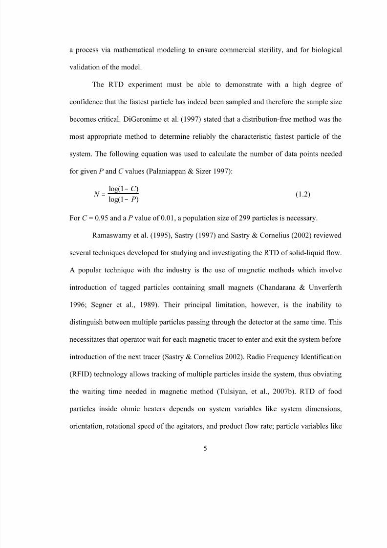
The RTD experiment must be able to demonstrate with a high degree of
confidence that the fastest particle has indeed been sampled and therefore the sample size
becomes critical. DiGeronimo et al. (1997) stated that a distribution-free method was the
most appropriate method to determine reliably the characteristic fastest particle of the
system. The following equation was used to calculate the number of data points needed
for given P and C values (Palaniappan & Sizer 1997):
N C
P =
−
−
log( )log( )
11
(1.2)
For C = 0.95 and a P value of 0.01, a population size of 299 particles is necessary.
Ramaswamy et al. (1995), Sastry (1997) and Sastry & Cornelius (2002) reviewed
several techniques developed for studying and investigating the RTD of solid-liquid flow.
A popular technique with the industry is the use of magnetic methods which involve
introduction of tagged particles containing small magnets (Chandarana & Unverferth
1996; Segner et al., 1989). Their principal limitation, however, is the inability to
distinguish between multiple particles passing through the detector at the same time. This
necessitates that operator wait for each magnetic tracer to enter and exit the system before
introduction of the next tracer (Sastry & Cornelius 2002). Radio Frequency Identification
(RFID) technology allows tracking of multiple particles inside the system, thus obviating
the waiting time needed in magnetic method (Tulsiyan, et al., 2007b). RTD of food
particles inside ohmic heaters depends on system variables like system dimensions,
orientation, rotational speed of the agitators, and product flow rate; particle variables like
5
5/9/2018 Sarang Sanjay S - slidepdf.com
http://slidepdf.com/reader/full/sarang-sanjay-s 24/170
concentration, shape, size, type, and density; and the fluid viscosity. There is a need to
study, in detail, the effect of these variables on the RTD in the ohmic heaters.
1.1 Nomenclature
C confidence of collecting the “fastest” particle fraction
N population size
P “fastest” particle fraction
V voltage across the sample (V)
u&
specific internal energy generation rate (W/m
3
)
σ electrical conductivity (S/m)
1.2 References
de Alwis, A. A. P., Halden, K. & Fryer, P. J. (1989). Shape and conductivity effects in
the ohmic heating of foods. Chemical Engineering Research, 67, 1547-1559
de Alwis, A. A. P. & Fryer, P. J. (1990). A finite element analysis of heat generation and
transfer during ohmic heating of food. Chemical Engineering Science, 45 (6), 1547-
1559
Chandarana, D. I. & Unverferth, J. A. (1996). Residence time distribution of particulate
foods at aseptic processing temperatures. Journal of Food Engineering 28, 349–360.
Del Valle, F. R., & Nickerson, J. T. R. (1967a). Studies on salting and drying fish. 1.
Equilibrium considerations in salting. Journal of Food Science, 32, 173-179.
Del Valle, F. R., & Nickerson, J. T. R. (1967b). Studies on salting and drying fish. 2.
Dynamic aspects of the salting of fish. Journal of Food Science, 218-224.
6
5/9/2018 Sarang Sanjay S - slidepdf.com
http://slidepdf.com/reader/full/sarang-sanjay-s 25/170
7
Drusas, A., & Vagenas, G. K. (1988). Diffusion of sodium chloride in green olives.
Journal of Food Engineering , 7, 211-222.
DiGeronimo, M., Garthright, W. & Larkin J. (1997). Statistical design and analysis. Food
Technology 51(10), 52–54.
Dussap, G., & Gros, J. B. (1980). Diffusion sorption model for salt in pork and beef
muscle. In, P. Linko, Y. Malkki, J. Olkku, & J. Laringkari (Eds), Food Process
Engineering (pp. 407-411). Applied Science Publishers, London.
Fryer, P. J., deAlwis, A. A. P., Koury, E., Stapley, A. G. F. & Zhang, L. (1993). Ohmic
processing of solid-liquid mixtures: heat generation and convection effects. Journal
of Food Engineering, 18, 101-125.
Khalaf, W. G. & Sastry, S. K. (1996). Effect of fluid viscosity on the ohmic heating rate
of solid-liquid mixtures. Journal of Food Engineering, 27, 125-158.
Larkin, J. W., & Spinak, S. H. (1996). Safety considerations of ohmically heated,
aseptically processed, multiphase low-acid food products. Food Technology, 242-
245.
Liu, H. (1992). A kinetic study of salt diffusion in potato at high temperature.
International Journal of Food Science and Technology, 27, 443-455.
Mitchell, F. R. G. & deAlwis, A. A. P. (1989). Electrical conductivity meter for food
particles. Journal of Physics E , 22, 554-556.
Orangi, S., Sastry, S. K. & Li, Q. (1997). A numerical investigation of electroconductive
heating in solid-liquid mixtures. International Journal of Heat and Mass Transfer, 41
(14), 2211-2220.

5/9/2018 Sarang Sanjay S - slidepdf.com
http://slidepdf.com/reader/full/sarang-sanjay-s 26/170
8
Palaniappan, S. & Sastry, S. (1991). Electrical conductivities of selected solid foods
during ohmic heating. Journal of Food Process Engineering , 14, 221-136
Palaniappan, S. & Sastry, S. (2002). Ohmic heating. In Control of Foodborne
Microorganisms, Eds. V. K. Juneja & J. N. Sofos. New York: Marcel Dekker, 451-
460.
Palaniappan, S., & Sizer, C. E. (1997). Aseptic process validation for food containing
particulates. Food Technology, 51(8), 60-68.
Ramaswamy, H. S., Abdelrahim, K. A., Simpson, B. K. & Smith, J. P. (1995). Residence
time distribution (RTD) in aseptic processing of particulate foods: a review. Food Res
Int 28(3), 291–310.
Ruhlman, K. T., Jin, Z. T. & Zhang, Q. H. (2001) Physical properties of liquid foods for
pulsed electric field treatment. In Pulsed Electric Fields in Food Processing. Eds.
Barbosa-Canovas, G. V. & Zhang, Q. H. Technomic Publishing Co., Lancaster, PA.,
45-56.
de Ruyter, P. W. & Brunet, R. (1973) Estimation of process conditions for the continuous
sterilization of foods containing particulates. Food Technology, 27(7), 44-51.
Sastry, S. K. (1992). A model for heating of liquid-particle mixtures in a continuous flow
ohmic heater. Journal of Food Process Engineering, 15, 263-278
Sastry S. K. (1997). Measuring residence time and modeling the system. Food
Technology 51(10), 44–48.
Sastry, S. K. & Palaniappan, S. (1992 a). Ohmic heating of liquid-particle mixtures. Food
Technology, 46 (12), 64-67.
5/9/2018 Sarang Sanjay S - slidepdf.com
http://slidepdf.com/reader/full/sarang-sanjay-s 27/170
9
Sastry, S. K. & Palaniappan, S. (1992 b). Influence of particle orientation on the effective
electrical resistance and ohmic heating rate of a liquid-particle mixture Journal of
Food Process Engineering, 15, 213-227.
Sastry, S. K. & Palaniappan, S. (1992 c). Mathematical modeling and experimental
studies on ohmic heating of liquid-particle mixtures in a static heater. Journal of Food
Process Engineering, 15, 241-261.
Sastry, S. K. & Li, Q. (1996). Modeling the ohmic heating of foods. Food Technology. 50
(5), 246-248.
Sastry, S. K. & Salengke, S. (1998). Ohmic heating of solid-liquid mixtures: A
comparison of mathematical models under worst-case heating conditions. Journal of
Food Process Engineering, 21, 441-458.
Sastry, S. K. & Cornelius, B. D., (2002) Aseptic processing of foods containing solid
particulates. Jon Wiley and Sons, Inc. New York. 2002.
Segner, W. P., Ragusa, T. J., Marcus, C. L. & Soutter, E. A. (1989). Biological evaluation
of a heat transfer simulation for sterilizing low-acid large particulate foods for aseptic
packaging. Journal of Food Processing and Preservation, 13, 257–274.
Sensoy, I. (2002) Ohmic and moderate electric field treatment of foods: studies on heat
transfer modeling, blanching, drying, rehydration and extraction. Thesis (PhD) Ohio
State University, 2002.
Tulsiyan, P., Sarang, S., & Sastry, S. K. (2007a). Electrical conductivity of
multicomponent systems during ohmic heating. International Journal of Food
Properties, (accepted).
5/9/2018 Sarang Sanjay S - slidepdf.com
http://slidepdf.com/reader/full/sarang-sanjay-s 28/170
10
Tulsiyan, P., Sarang, S., & Sastry, S. K. (2007b). Radio Frequency Identification:
Residence Time Distribution of a Multicomponent System inside Ohmic Heater.
Journal of Food Science, (submitted).
Wang, W. & Sastry, S. (1993 a). Salt diffusion into vegetable tissue as a pretreatment for
ohmic heating: electrical conductivity profiles and vacuum infusion studies. Journal
of Food Engineering, 20, 299-309.
Wang, W. & Sastry, S. (1993 b). Salt diffusion into vegetable tissue as a pretreatment for
ohmic heating: determination of parameters and mathematical model verification.
Journal of Food Engineering, 20, 311-323.
Wistreich, H. E., Morse, R. E., & Kenyon, L. J. (1960) Curing of ham: a study of sodium
chloride accumulation. II: Combined effects of time, solution concentration and
solution volume. Food Technology, 14, 549-551.
Wood, F. W. (1966). The diffusion of salt in pork muscle and fat tissue. Journal of the
Science of Food and Agriculture, 17, 138-140.
Zhang, L. & Fryer, P. J. (1993). Models for the electrical heating of solid-liquid mixtures.
Chemical Engineering Science. 48, 633-643
5/9/2018 Sarang Sanjay S - slidepdf.com
http://slidepdf.com/reader/full/sarang-sanjay-s 29/170
11
CHAPTER 2
ELECTRICAL CONDUCTIVITY OF FRUITS AND MEATS DURING OHMIC
HEATING
2.1 Abstract
The design of effective ohmic heaters depends on the electrical conductivity of
foods. Electrical conductivities of six different fresh fruits (red apple, golden apple,
peach, pear, pineapple and strawberry) and several different cuts of three types of meat
(chicken, pork and beef) were determined from room temperature through the
sterilization temperature range (25 -140oC). In all cases, conductivities increased linearly
with temperature. In general, fruits were less conductive than meat samples. Within
fruits; peach and strawberry were more conductive than apples, pear, and pineapple.
Conductivity measurements of meat cuts showed that lean is much more conductive
compared to fat. Fat content of all lean muscle cuts was measured and no strong
relationship could be observed between the electrical conductivity and the lean muscle fat
content.
.
5/9/2018 Sarang Sanjay S - slidepdf.com
http://slidepdf.com/reader/full/sarang-sanjay-s 30/170
2.2 Introduction
In ohmic or electroconductive heating, foods are heated by passing alternating
current through them. Most foods contain ionic species such as salts and acids, hence,
electric current can be made to pass through the food and generate heat inside it
(Palaniappan & Sastry, 1991). A large number of potential applications exist for ohmic
heating, including blanching, evaporation, dehydration, fermentation, and extraction. In
case of the application as heat treatment for microbial control ohmic heating provides
rapid and uniform heating, resulting in less thermal damage to the product. A high-
quality product with minimal structural, nutritional, or organoleptic changes can be
manufactured in a short operating time (Rahman, 1999). Ohmic heating is currently being
used for the processing of whole fruits, syruped fruit-salad and fruit juices in Japan and
the United Kingdom. Ohmic heating has shown to enhance drying rates (Lima & Sastry,
1999; Wang & Sastry, 2000; Zhong & Lima, 2003) and extraction yields (Lima & Sastry,
1999; Wang & Sastry, 2002; Halden, de Alwis & Fryer, 1990) in certain fruits and
vegetables.
The rate of heating is directly proportional to the electrical conductivity and the
square of the electric field strength (Sastry & Palaniappan, 1992). Palaniappan and Sastry
(1991) reported that electrical conductivity is a linear function of temperature, and the
relationship can be expressed as:
12
)⎤⎦ (2.1)(1T ref ref m T T σ σ ⎡= + −⎣
Much research has been done on the electrical conductivity of liquid fruit products like
juices and purees (Palaniappan & Sastry, 1991; Icier & Ilicali, 2005; Castro, Teixeira,
Salengke, Sastry & Vicente, 2004). Mitchell & de Alwis (1989) measured electrical
5/9/2018 Sarang Sanjay S - slidepdf.com
http://slidepdf.com/reader/full/sarang-sanjay-s 31/170
13
conductivity of pear and apple at 25oC. Castro, Teixeira, Salengke, Sastry & Vicente
(2003) reported electrical conductivity of fresh strawberry over 25-100oC temperature
range.
Electrical properties of meat have also been investigated in recent years (Saif,
Lan, Wang & Garcia, 2004). Conductivities of chicken (Mitchell & de Alwis, 1989;
Palaniappan & Sastry, 1991) beef (Kim, Kim, Park, Cho & Han, 1996; Palaniappan &
Sastry, 1991) and pork (Halden, de Alwis, & Fryer, 1990) have been measured, but the
type of meat cut was not specified. Tulsiyan, Sarang & Sastry (2007) measured
conductivity of chicken breast over the sterilization temperature range. Shirsat, Lyng,
Brunton & McKenna (2004) reported conductivities of different pork cuts and observed
that lean is highly conductive compared to fat, however, conductivity measurements were
performed only at 20oC.
The aim of this study was to measure electrical conductivity of selected fresh
fruits (red apple, golden apple, peach, pear, pineapple and strawberry) and different cuts
of fresh meat (chicken, pork and beef) over the sterilization temperature range during
ohmic heating.
2.3 Materials and methods
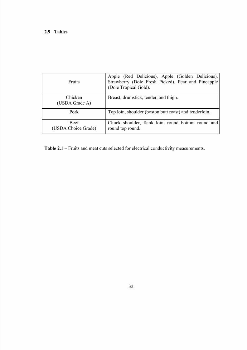
Listed in Table 2.1, are the several fruits and meat cuts that were studied. Meat
cuts were selected to cover different parts of the animal, and to represent various fat
contents (USDA Handbook 8, 2005). Samples were procured from local grocery store
(Giant Eagle, Columbus, OH) and refrigerated until used. Except for the case of chicken
5/9/2018 Sarang Sanjay S - slidepdf.com
http://slidepdf.com/reader/full/sarang-sanjay-s 32/170
14
fat, all meat cuts were trimmed to separate lean from fat to ensure that only the
conductivity of lean was measured.
2.3.1 Electrical conductivity
2.3.1.1 Experimental device
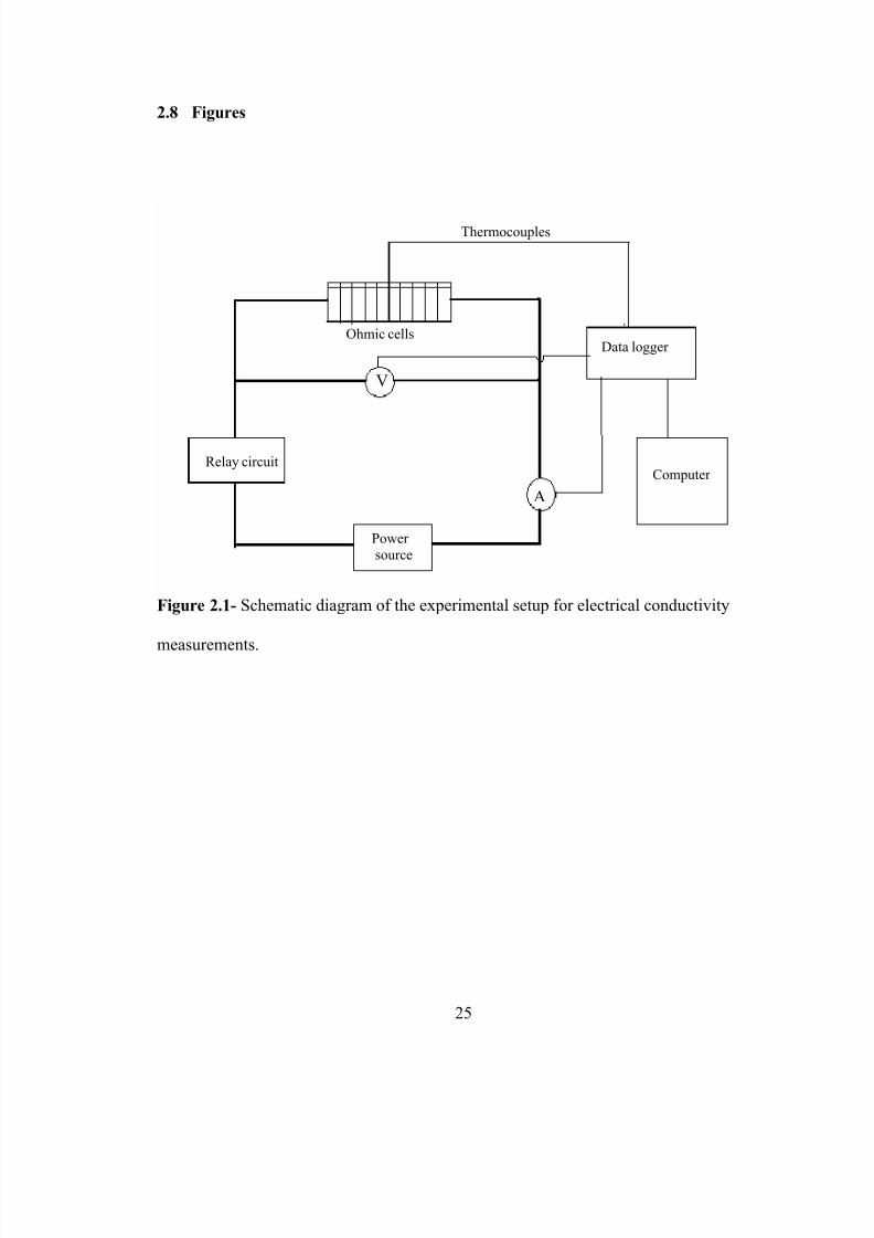
The setup, explained in detail elsewhere (Tulsiyan, Sarang & Sastry, 2007),
consisted of ten cylindrical ohmic heating chambers equipped with platinized titanium
electrodes. The device was pressurized, and allowed measurement of the electrical
conductivity of ten samples at a time and at temperatures up to 140
o
C. A schematic
diagram of the electrical circuitry is shown in Fig. 2.1. Samples were clamped at the ends
by two electrodes in each cell, and a T-type copper-constantan, Teflon coated
thermocouple (Cleveland Electric Laboratories, Twinsburg, OH) with compression fitting
was used to measure the temperature at the geometric center of the sample. The ohmic
cells were connected to a relay switch which directed the order in which the cells were
heated. Voltage and current transducers were used to measure the voltage across the
samples and the current flowing through them. A data logger (Campbell Scientific Inc.,
Logan, UT) was used to record data at constant time intervals.
2.3.1.2 Methodology
Cylindrical samples of fruits and meat (ten samples each) were prepared using a
slicer and a set of cork borers. The samples were 0.0079m (0.313”) in length and
0.0078m (0.308”) in diameter. Samples may shrink and loose contact with the electrodes
when ohmically heated to higher temperatures, hence, samples of the same diameter but
fractionally longer compared to the sample chamber were prepared and sandwiched
5/9/2018 Sarang Sanjay S - slidepdf.com
http://slidepdf.com/reader/full/sarang-sanjay-s 33/170
between the electrodes. All the meat samples were cut perpendicular to the muscle
fibers, so that the muscle fibers would be perpendicular to the electric field. A
thermocouple was then inserted into the cell through the thermocouple port and each
sample was heated to 140oC using alternating current of 60 Hz and voltage between 15 to
20V. The temperature, voltage and current were measured continuously and recorded
using the data logger linked to the computer. It was difficult to get cylindrical sample of
the meat separable fat of required dimensions, and the conductivities were measured by
packing as much as fat possible in the sample chamber.
2.3.1.3 Analysis
The electrical conductivity of the samples was calculated using the dimensions of
the cell, voltage and the current, using the formula:
LI
AV σ =
(2.2)
2.3.1.4 Error estimation
The accuracy of each electrode set was tested, before and after the experiments,
by determining the electrical conductivity of three different calibration salt solutions
(conductivity standard solution 8974 μS/cm, 12880 μS/cm & 15000 μS/cm, OAKTON
Instruments, Vernon Hills, IL, USA). The maximum difference between the measured
and the reference value for any heating cell was 9%. The temperature at the center of the
sample was used as the representative value, and was assumed to be spatially uniform
because of the small size of the sample.
15
5/9/2018 Sarang Sanjay S - slidepdf.com
http://slidepdf.com/reader/full/sarang-sanjay-s 34/170
16
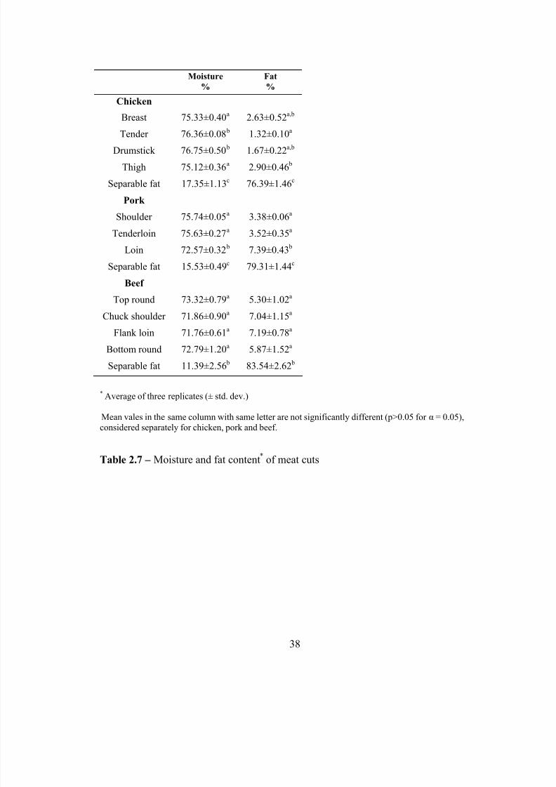
2.3.2 Fat analysis of meat
Fat and moisture content of the meat was determined using HFT 2000f DSC
(Data Support Company Inc., Encino, CA) fat and moisture analyzer (accuracy is ± 0.5%
range of 1%). Fat and moisture content was measured for three replicate runs for each
sample. For each replicate, first 50 grams of sample was fine ground using
Mincer/Chopper HC 20 (Black & Decker Inc., Shelton, CT) and 3-4 grams of sample was
then used for analysis.
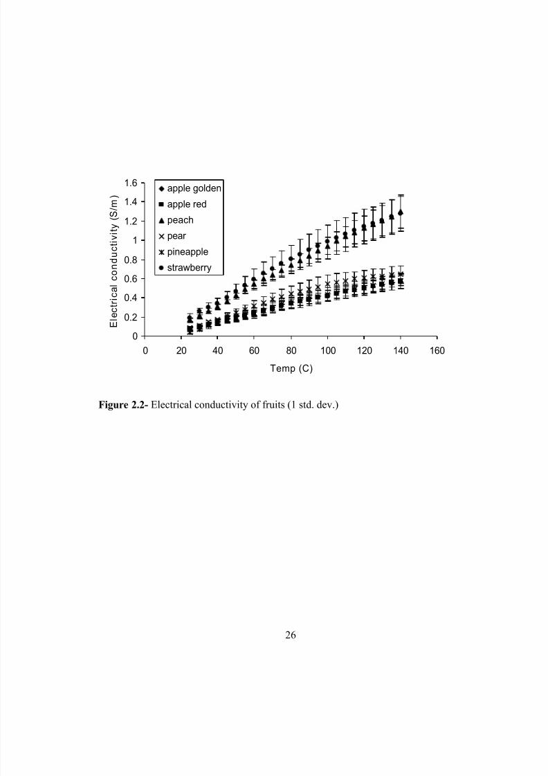
2.4 Results and discussion
Electrical conductivity-temperature curves for selected fresh fruits, and different
cuts of chicken, pork and beef are shown in Fig. 2.2, through Fig. 2.5, respectively. Y-
error bars shown are single standard deviations. The conductivity data is also summarized
for selected temperatures in Table 2.2, through Table 2.5. The conductivity data was
subjected to analysis of variance (ANOVA) and mean values in the same row with the
same letter are not significantly different (p>0.05 for α = 0.05). For all samples, electrical
conductivity increased almost linearly with temperature, as is expected and consistent
with literature data (Palaniappan & Sastry, 1991; Castro, et al., 2003; Tulsiyan, Sarang &
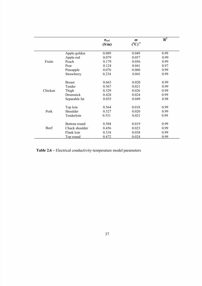
Sastry, 2007). The linear model (equation 2.1) by Palaniappan & Sastry (1991) was used
to fit the electrical conductivity data of fruit and meat samples. m, σ ref and R2
values are
shown in Table 2.6. High coefficients of determination (R
2
>0.97) indicate the suitability
of the linear model for conductivity variation with temperature for all the samples tested.
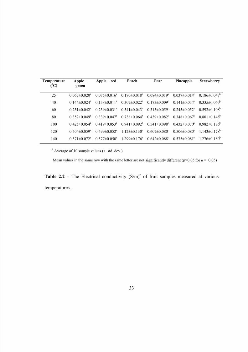
From Table 2.2 it can be observed that the electrical conductivities of red apple
and golden apple were not significantly different over the temperature range studied, and
5/9/2018 Sarang Sanjay S - slidepdf.com
http://slidepdf.com/reader/full/sarang-sanjay-s 35/170
17
hereafter mentioned together as apples. At 25oC the electrical conductivity of pineapple
was very low and significantly different than apples and pear. Electrical conductivity of
peach and strawberry was high and not significantly different compared to each other,
while significantly different compared to other fruits. At higher temperatures (40-140oC),
apples and pineapple had low conductivity. Conductivity of pear was high compared to
apples and pineapple and significantly different compared to all other fruits. Strawberry
and peach had higher conductivity and significantly different compared to other fruits.
The gap in the electrical conductivity between strawberry and peach, and other fruits
increased with the temperature. Mavroudis et al. (2004) and Rahman et al. (2005)
measured porosity of fresh apples and observed that the porosity can be as high as 20%.
The presence of large amount of air might explain low conductivity of apple tissues.
Mitchell & de Alwis (1989) reported conductivity of pear (0.041 S/m) and apple (0.023
S/m) at 25oC. From Table 2.2, it can be observed that the conductivity at 25
oC of pear is
0.084 S/m, red apple is 0.075 S/m and of golden apple is 0.067 S/m. Mitchell & de
Alwis (1989) measured conductivity at 50 Hz while we used 60 Hz supply, which might
explain the difference in the measured electrical conductivity of pear and apple samples.
Castro, et al. (2003) measured electrical conductivity of fresh strawberries at different
field strengths. At 25 V/cm they reported conductivity to be approximately 0.05 S/m at
25oC and 0.55 S/m at 100
oC, and it increased linearly. From Table 2.2, it can be observed
that conductivity of strawberry increased from 0.186 S/m at 25
o
C to about 0.982 S/m at
100oC. Again these researchers measured conductivity using 50 Hz power supply and
higher field strength. Difference in the power source and the natural variation among the
species might explain the difference in the electrical conductivities observed.
5/9/2018 Sarang Sanjay S - slidepdf.com
http://slidepdf.com/reader/full/sarang-sanjay-s 36/170
18
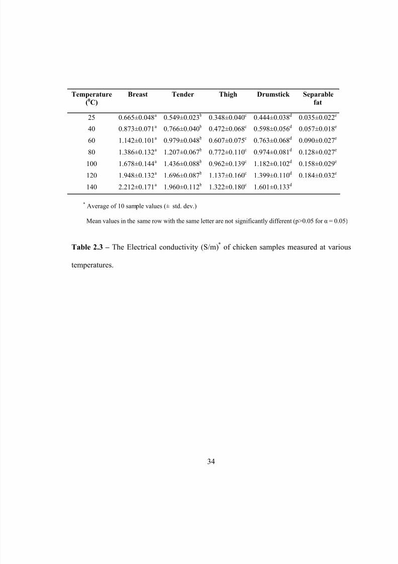
Fig. 2.3 shows conductivity of different cuts of chicken and the data is
summarized in Table 2.3. It can be observed that separable fat is the least conductive. At
all temperatures lean chicken breast is most conductive and that the conductivities of
different cuts are significantly different from each other. It was difficult to obtain
conductivity data for chicken separable fat at higher temperatures without spoiling
(damaging the coating) the electrodes. Thus, conductivity was measured only till 135oC.
Also, to preserve the electrodes, conductivity of pork and beef separable fat was not
determined. It may be safely assumed that separable fat will be significantly lower in
conductivity compared to lean muscle cuts. Fat and moisture content (percent by weight)
of chicken cuts were measured and are summarized in Table 2.7. In Fig 2.6, electrical
conductivity of chicken muscle cuts are plotted against their average fat content at 25oC
and at 140oC. It may be observed that electrical conductivity reduced with increase in the
total fat content. However, it can also be observed that chicken breast contains more fat
but still is more conductive than tenders and drumstick.
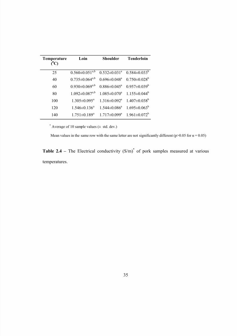
Electrical conductivity variation with temperature of three different cuts of lean
pork muscles is shown in Fig. 2.4 and the data is summarized in Table 2.4. At higher
temperatures (above 100oC) tenderloin is more conductive than loin and shoulder.
Measured fat content of pork cuts are shown in Table 2.7. Top loin contains more fat
compared to shoulder and tenderloin, however the conductivity data (Table 2.4) shows
that tenderloin is more conductive than top loin and shoulder. For pork cuts no particular
trend could be observed between the conductivity and the total fat content. Shirsat, et al.
(2004) measured electrical conductivity of fresh pork cuts of leg (topside), shoulder
(picnic), and back and belly fat. They reported that lean is highly conductive compared
5/9/2018 Sarang Sanjay S - slidepdf.com
http://slidepdf.com/reader/full/sarang-sanjay-s 37/170
19
to fat. They also observed that the conductivity of leg (fat content 0.4%) and shoulder (fat
content 0.9%) was significantly different, but conductivity of shoulder and belly (fat
content 2.3%) was not significantly different. They concluded that in addition to the fat
content the structural differences may influence the conductivity of muscles.
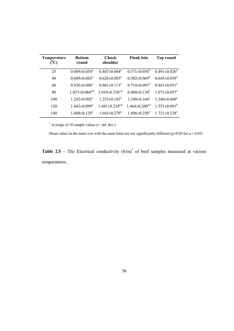
Fig. 2.5 shows conductivity of different lean cuts of beef and the data is
summarized in Table 2.5. At lower temperatures (up to 60oC) flank loin had lowest
conductivity and significantly different compared to other muscle cuts, while at higher
temperatures the conductivities of all cuts were almost similar. Beef cuts showed
considerable variation and were not significantly different in terms of the measured fat
content (see Table 2.7).
Increase in the electrical conductivity during heating of the biological tissue
occurs due to increase in the ionic mobility because of structural changes in the tissue
like cell wall protopectin breakdown, expulsion of non conductive gas bubbles, softening,
and lowering in aqueous phase viscosity (Bean, Rasor & Porter, 1960; Sasson &
Monselise, 1977). Higher electrical conductivity of strawberry and peach may be
attributed to the softer tissues and hence higher ionic mobility in comparison to the harder
tissues of apples, pineapple and pear. Also, as mentioned earlier, presence of large
amount of air might result in lower electrical conductivity of apple tissues. The other
most important factor influencing the conductivity is the total ionic content of these
fruits. Measurement of the total ionic content - sugars and salts - and comparison of the
conductivity based on the ionic contents is a topic for future study. In meat, the separable
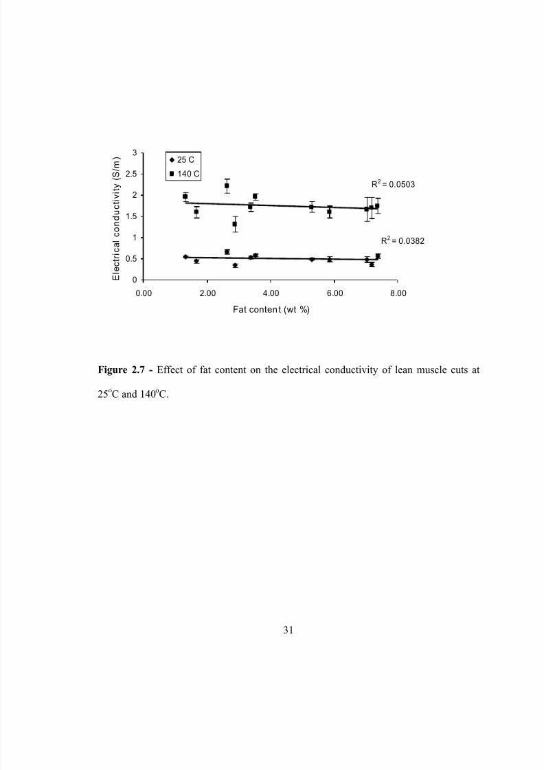
fat has significantly lower conductivity compared to lean muscle cuts. In Fig.2.7,
electrical conductivities of the lean muscle cuts at 25oC and at 140
oC are plotted against
5/9/2018 Sarang Sanjay S - slidepdf.com
http://slidepdf.com/reader/full/sarang-sanjay-s 38/170
20
their fat content (mean values). Linear regression analysis gave R 2
= 0.038 at 25oC, and
0.050 at 140oC. Thus, within the lean muscle cuts it is difficult to find any relationship
between the electrical conductivity and measured muscle fat content. Salengke & Sastry
(2007a,b) and Sastry & Palaniappan (1992) performed mathematical modeling and
experimental investigation of the case where less conductive particle is surrounded by
high conductive medium and heated ohmically under static condition. They observed that
the current channels through a more conductive medium and may bypass the less
conductive particle. Also, the presence or absence of the alternative conducting paths
through the surrounding medium is an important factor affecting voltage drops and
consequently, energy generation rates within both media. Similar explanation might be
offered when a low conductive fat is surrounded by high conductive muscle tissues. In
addition to the conductivity difference, the size and the distribution of the non conductive
fat in the muscle tissues might play an important role. In summary, for lean muscle cuts
marbling (fat distribution) may be an important factor affecting the electrical
conductivity; which needs further investigation.
2.5 Conclusions
The electrical conductivity of various fruits and meats increased linearly with the
temperature during ohmic heating at constant voltage gradient. Lower electrical
conductivity may be observed for highly porous materials like apples. There was no
strong relationship between the measured fat content of the lean muscle cuts and their
electrical conductivity. Fat distribution or marbling might be an important factor affecting
the electrical conductivity of meat.
5/9/2018 Sarang Sanjay S - slidepdf.com
http://slidepdf.com/reader/full/sarang-sanjay-s 39/170
2.6 Nomenclature
A cross sectional area of the sample (m2)
I current flowing through the sample (A)
L length of the sample (m)
m temperature compensation constant
T temperature (oC)
T ref reference temperature (oC)
V voltage across the sample (V)
σ electrical conductivity (S/m)
σ ref electrical conductivity at reference temperature (S/m)
σ T electrical conductivity at any temperature (S/m)
2.7 References
Bean, E. C., Rasor, J. P., & Porter, G.C. (1960). Changes in electrical conductivities of
avocados during ripening. Year Book of Californian Avocado Society, 44, 75–78.
Castro, I., Teixeira, J. A., Salengke, S., Sastry, S. K., & Vicente, A. A. (2003). The
influence of field strength, sugar and solid content on electrical conductivity of
strawberry products. Journal of Food Process Engineering, 26, 17-29.
Castro, I., Teixeira, J. A., Salengke, S., Sastry, S. K. & Vicente, A. A. (2004). Ohmic
heating of strawberry products: electrical conductivity measurements and ascorbic
acid degradation kinetics. Innovative Food Science and Engineering Technologies, 5,
27-36.
21
5/9/2018 Sarang Sanjay S - slidepdf.com
http://slidepdf.com/reader/full/sarang-sanjay-s 40/170
22
Halden, K., de Alwis, A. A. P., & Fryer, P.J. (1990). Changes in the electrical
conductivity of foods during ohmic heating. International Journal of Food Science
and Technology, 25(1), 9–25.
Icer, F., & Ilicali, C. (2005). Temperature dependent electrical conductivities of fruit
purees during ohmic heating. Food Research International, 38, 1135-1142.
Kim, S. H., Kim, G. T., Park, J. Y. Cho, M. G., & Han, B. H. (1996). A study on the
ohmic heating of viscous food. Foods and Biotechnology, 5(4), 274-279.
Lima, M., & Sastry, S. K. (1999). The effect of ohmic heating frequency on hot-air
drying rate and juice yield. Journal of Food Engineering, 41, 115-119.
Mavroudis, N. E., Dejmek, P., & Sjoholm, I. (2004). Studies on some raw material
characteristics in different Swedish apple varieties. Journal of Food Engineering , 62,
121-129.
Mitchell, F. R. G., & de Alwis, A. A. P. (1989). Electrical conductivity meter for food
samples. Journal of Physics. E ., 22, 554–556.
Palaniappan, S., & Sastry, S. K. (1991). Electrical conductivities of selected solid foods
during ohmic heating. Journal of Food Process Engineering , 14, 221-136.
Rahman, M. S. (1999). In Rahman, M. S., (Ed.), Handbook of Food Preservation; (pp.
521-532). Dekker: New York.
Rahman, M. S., Al-Zakwani, I., & Guizani, N. (2005). Pore formation in apple during air-
drying as a function of temperature: porosity and pore-size distribution. Journal of the
Science of Food and Agriculture, 85, 979-989.
Saif, S. M. H., Lan, Y., Wang, S., & Garcia, S. (2004). Electrical resistivity of goat meat.
International Journal of Food Properties, 7(3), 463-471.
5/9/2018 Sarang Sanjay S - slidepdf.com
http://slidepdf.com/reader/full/sarang-sanjay-s 41/170
23
Salengke, S., & Sastry, S. K. (2007a). Experimental investigation of ohmic heating of
solid-liquid mixtures under worst-case heating scenarios. Journal of Food
Engineering, 83 (3), 324-336.
Salengke, S., & Sastry, S. K. (2007b). Models for ohmic heating of solid-liquid mixtures
under worst-case heating scenarios. Journal of Food Engineering, 83 (3), 337-355.
Sasson, A., & Monselise, A. P. (1977). Electrical conductivity of ’shamouti’ orange peel
during fruit growth and postharvest senescence. Journal of American Society:
Horticulture Science, 102(2), 142–144.
Sastry, S. K., & Palaniappan, S. (1992). Mathematical modeling and experimental studies
on ohmic heating of liquid-particle mixtures in a static heater. Journal of Food
Process Engineering, 15, 241–261.
Shirsat, N., Lyng, J. G., Brunton, N. P., & McKenna, B. (2004). Ohmic processing:
Electrical conductivities of pork cuts. Meat Science, 67, 507-514.
Tulsiyan, P., Sarang, S., & Sastry, S. K. (2007). Electrical conductivity of
multicomponent systems during ohmic heating. International Journal of Food
Properties, (accepted).
U.S. Department of Agriculture, Agricultural Research Service. (2005). USDA Nutrient
Database for Standard Reference, Release 18. Nutrient Data Laboratory Home Page,
http://www.nal.usda.gov/fnic/foodcomp
Wang, W. C., & Sastry, S. K. (2000). Effects of thermal and electrothermal pretreatments
on hot air drying rate of vegetable tissue. Journal of Food Process Engineering , 23,
299-219.
5/9/2018 Sarang Sanjay S - slidepdf.com
http://slidepdf.com/reader/full/sarang-sanjay-s 42/170
24
Wang, W. C., & Sastry, S. K. (2002). Effects of moderate electrothermal treatments on
juice yield from cellular tissue. Innovative Food Science and Emerging Technologies,
3(4), 371-377.
Zhong, T., & Lima, M. (2003). The effect of ohmic heating on vacuum drying rate of
sweet potato tissue. Bioresource Technology, 87, 215-220.
5/9/2018 Sarang Sanjay S - slidepdf.com
http://slidepdf.com/reader/full/sarang-sanjay-s 43/170
2.8 Figures
Thermocouples
Ohmic cellsData logger
V
Relay circuitComputer
A
Power
source
Figure 2.1- Schematic diagram of the experimental setup for electrical conductivity
measurements.
25
5/9/2018 Sarang Sanjay S - slidepdf.com
http://slidepdf.com/reader/full/sarang-sanjay-s 44/170
0
0.2
0.4
0.6
0.8
1
1.2
1.4
1.6
0 20 40 60 80 100 120 140 160
Temp (C)
E l e c t r i c a l c o n d u c t i v i t y ( S / m )
apple golden
apple red
peach
pear
pineapple
strawberry
Figure 2.2- Electrical conductivity of fruits (1 std. dev.)
26
5/9/2018 Sarang Sanjay S - slidepdf.com
http://slidepdf.com/reader/full/sarang-sanjay-s 45/170
0
0.5
1
1.5
2
2.5
0 20 40 60 80 100 120 140 160Temp (C)
E l e c t r i c a l c o n d u c t i v i t y ( S / m ) breast
tender
drumstick
thigh
separable fat
Figure 2.3- Electrical conductivity of different cuts of chicken (1 std. dev.)
27
5/9/2018 Sarang Sanjay S - slidepdf.com
http://slidepdf.com/reader/full/sarang-sanjay-s 46/170
0
0.5
1
1.5
2
2.5
0 20 40 60 80 100 120 140 160
Temp (C)
E l e c t r i c a l c o n d u c t i v i t y ( S / m )
loin
tenderloin
shoulder
Figure 2.4- Electrical conductivity of different pork cuts (1 std. dev.)
28
5/9/2018 Sarang Sanjay S - slidepdf.com
http://slidepdf.com/reader/full/sarang-sanjay-s 47/170
0
0.5
1
1.5
2
2.5
0 20 40 60 80 100 120 140 160
Temp (C)
E
l e c t r i c a l c o n d u c t i v i t y ( S / m ) top round
chuck shoulder
flank loin
bottom round
Figure 2.5- Electrical conductivity of different beef cuts (1 std. dev.)
29
5/9/2018 Sarang Sanjay S - slidepdf.com
http://slidepdf.com/reader/full/sarang-sanjay-s 48/170
0
0.5
1
1.5
2
2.5
3
0.0 0.5 1.0 1.5 2.0 2.5 3.0 3.5
Fat content (wt %)
E l e c t r i c a l c o n d u c t i v i t y ( S / m
)
25 C
140 C
Breast
Figure 2.6 - Effect of fat content on the electrical conductivity of chicken cuts at 25oC
and 140oC.
30
5/9/2018 Sarang Sanjay S - slidepdf.com
http://slidepdf.com/reader/full/sarang-sanjay-s 49/170
R2 = 0.0503
R2
= 0.0382
0
0.5
1
1.5
2
2.5
3
0.00 2.00 4.00 6.00 8.00
Fat content (wt %)
E l e
c t r i c a l c o n d u c t i v i t y ( S / m ) 25 C
140 C
Figure 2.7 - Effect of fat content on the electrical conductivity of lean muscle cuts at
25oC and 140
oC.
31
5/9/2018 Sarang Sanjay S - slidepdf.com
http://slidepdf.com/reader/full/sarang-sanjay-s 50/170
32
2.9 Tables
Fruits
Apple (Red Delicious), Apple (Golden Delicious),
Strawberry (Dole Fresh Picked), Pear and Pineapple
(Dole Tropical Gold).
Chicken
(USDA Grade A)
Breast, drumstick, tender, and thigh.
Pork Top loin, shoulder (boston butt roast) and tenderloin.
Beef (USDA Choice Grade)
Chuck shoulder, flank loin, round bottom round andround top round.
Table 2.1 – Fruits and meat cuts selected for electrical conductivity measurements.
5/9/2018 Sarang Sanjay S - slidepdf.com
http://slidepdf.com/reader/full/sarang-sanjay-s 51/170
33
Temperature
(0C)
Apple –
green
Apple – red Peach Pear Pineapple Strawberry
25 0.067±0.020a 0.075±0.016a 0.170±0.018 b 0.084±0.019a 0.037±0.014c 0.186±0.047 b
40 0.144±0.024a 0.138±0.011a 0.307±0.022 b 0.173±0.009c 0.141±0.034a 0.335±0.060 b
60 0.251±0.042a 0.239±0.031a 0.541±0.043 b 0.313±0.059c 0.245±0.052a 0.592±0.108 b
80 0.352±0.049a 0.339±0.047a 0.738±0.064 b 0.439±0.082c 0.348±0.067a 0.801±0.148 b
100 0.425±0.054a 0.419±0.053a 0.941±0.092 b 0.541±0.098c 0.432±0.070a 0.982±0.176 b
120 0.504±0.059a 0.499±0.052a 1.123±0.130 b 0.607±0.080c 0.506±0.080a 1.143±0.178 b
140 0.571±0.072a 0.577±0.050a 1.299±0.176 b 0.642±0.088c 0.575±0.081a 1.276±0.180 b
* Average of 10 sample values (± std. dev.)
Mean values in the same row with the same letter are not significantly different (p>0.05 for α = 0.05)
Table 2.2 – The Electrical conductivity (S/m)*
of fruit samples measured at various
temperatures.
5/9/2018 Sarang Sanjay S - slidepdf.com
http://slidepdf.com/reader/full/sarang-sanjay-s 52/170
34
Temperature
(0C)
Breast Tender Thigh Drumstick Separable
fat
25 0.665±0.048a 0.549±0.023 b 0.348±0.040c 0.444±0.038d 0.035±0.022e
40 0.873±0.071a 0.766±0.040 b 0.472±0.068c 0.598±0.056d 0.057±0.018e
60 1.142±0.101a 0.979±0.048 b 0.607±0.075c 0.763±0.068d 0.090±0.027e
80 1.386±0.132a 1.207±0.067 b 0.772±0.110c 0.974±0.081d 0.128±0.027e
100 1.678±0.144a 1.436±0.088 b 0.962±0.139c 1.182±0.102d 0.158±0.029e
120 1.948±0.132a 1.696±0.087 b 1.137±0.160c 1.399±0.110d 0.184±0.032e
140 2.212±0.171a 1.960±0.112 b 1.322±0.180c 1.601±0.133d
* Average of 10 sample values (± std. dev.)
Mean values in the same row with the same letter are not significantly different (p>0.05 for α = 0.05)
Table 2.3 – The Electrical conductivity (S/m)*
of chicken samples measured at various
temperatures.
5/9/2018 Sarang Sanjay S - slidepdf.com
http://slidepdf.com/reader/full/sarang-sanjay-s 53/170
Temperature
35
(0C)
Loin Shoulder Tenderloin
25 0.560±0.051a,b 0.532±0.031a 0.584±0.033 b
40 0.735±0.064a,b 0.696±0.048a 0.750±0.028 b
60 0.930±0.069a,b 0.886±0.045a 0.957±0.039 b
80 1.092±0.087a,b 1.085±0.070a 1.155±0.044 b
100 1.305±0.095a 1.316±0.092a 1.407±0.038 b
120 1.546±0.136a 1.544±0.086a 1.695±0.063 b
140 1.751±0.189a 1.717±0.099a 1.961±0.072 b
* Average of 10 sample values (± std. dev.)
Mean values in the same row with the same letter are not significantly different (p>0.05 for α = 0.05)
Table 2.4 – The Electrical conductivity (S/m)*
of pork samples measured at various
temperatures.
5/9/2018 Sarang Sanjay S - slidepdf.com
http://slidepdf.com/reader/full/sarang-sanjay-s 54/170
Temperature
36
(0C)
Bottomround
Chuck shoulder
Flank loin Top round
25 0.489±0.054a 0.487±0.064a 0.371±0.050 b 0.491±0.026a
40 0.669±0.065a 0.626±0.085a 0.502±0.069 b 0.645±0.039a
60 0.826±0.086a 0.801±0.113a 0.710±0.091 b 0.841±0.051a
80 1.037±0.084a,b 1.019±0.156a,b 0.960±0.134 b 1.071±0.057a
100 1.242±0.092a 1.253±0.192a 1.240±0.166a 1.346±0.060a
120 1.443±0.099a 1.481±0.224a,b 1.464±0.200a,b 1.551±0.091 b
140 1.608±0.139a 1.665±0.279a 1.696±0.250a 1.721±0.128a
* Average of 10 sample values (± std. dev.)
Mean values in the same row with the same letter are not significantly different (p>0.05 for α = 0.05)
Table 2.5 – The Electrical conductivity (S/m)*
of beef samples measured at various
temperatures.
5/9/2018 Sarang Sanjay S - slidepdf.com
http://slidepdf.com/reader/full/sarang-sanjay-s 55/170
σref
(S/m)
m
(oC)
-1R
2
Apple-golden 0.089 0.049 0.99
Apple-red 0.079 0.057 0.99
Peach 0.179 0.056 0.99
Pear 0.124 0.041 0.97
Pineapple 0.076 0.060 0.99
Fruits
Strawberry 0.234 0.041 0.99
Breast 0.663 0.020 0.99
Tender 0.567 0.021 0.99
Thigh 0.329 0.026 0.99
Drumstick 0.428 0.024 0.99
Chicken
Separable fat 0.035 0.049 0.98
Top loin 0.564 0.018 0.99
Shoulder 0.527 0.020 0.99Pork
Tenderloin 0.551 0.021 0.99
Bottom round 0.504 0.019 0.99
Chuck shoulder 0.456 0.023 0.99
Flank loin 0.318 0.038 0.99
Beef
Top round 0.472 0.024 0.99
Table 2.6 – Electrical conductivity-temperature model parameters
37
5/9/2018 Sarang Sanjay S - slidepdf.com
http://slidepdf.com/reader/full/sarang-sanjay-s 56/170
Moisture
%
Fat
%
Chicken
38
Breast 75.33±0.40a 2.63±0.52a,b
Tender 76.36±0.08 b
1.32±0.10a
Drumstick 76.75±0.50 b 1.67±0.22a,b
Thigh 75.12±0.36a 2.90±0.46 b
Separable fat 17.35±1.13c 76.39±1.46c
Pork
Shoulder 75.74±0.05a 3.38±0.06a
Tenderloin 75.63±0.27a 3.52±0.35a
Loin 72.57±0.32 b 7.39±0.43 b
Separable fat 15.53±0.49c 79.31±1.44c
Beef
Top round 73.32±0.79a 5.30±1.02a
Chuck shoulder 71.86±0.90a 7.04±1.15a
Flank loin 71.76±0.61a 7.19±0.78a
Bottom round 72.79±1.20a 5.87±1.52a
11.39±2.56 bSeparable fat 83.54±2.62 b
* Average of three replicates (± std. dev.)
Mean vales in the same column with same letter are not significantly different (p>0.05 for α = 0.05),
considered separately for chicken, pork and beef.
Table 2.7 – Moisture and fat content*
of meat cuts

5/9/2018 Sarang Sanjay S - slidepdf.com
http://slidepdf.com/reader/full/sarang-sanjay-s 57/170
39
CHAPTER 3
BLANCHING AS A PRETREATMENT METHOD TO IMPROVE UNIFORMITY
IN HEATING OF SOLID-LIQUID FOOD MIXTURES
3.1 Abstract
The electrical conductivity of food components is critical to ohmic heating. Food
components of different electrical conductivities heat at different rates. While equal
electrical conductivities of all phases is desirable, real food products may behave
differently. In the present study involving chicken chowmein consisting of a sauce and
different solid components; celery, water chestnuts, mushrooms, bean sprouts and
chicken; it was observed that the sauce was more conductive than all solid components
over the measured temperature range. To improve heating uniformity, a blanching
method was developed to increase the ionic content of the solid components. By
blanching different solid components in a highly conductive sauce at 100oC for different
lengths of time, it was possible to adjust their conductivity to that of the sauce. Chicken
chowmein samples containing blanched particulates were compared with untreated
samples with respect to ohmic heating uniformity at 60-Hz up to 140
o
C. All components
of the treated product containing blanched solids heated more uniformly than untreated
product. In sensory tests, three different formulations of the blanched product showed
5/9/2018 Sarang Sanjay S - slidepdf.com
http://slidepdf.com/reader/full/sarang-sanjay-s 58/170
good quality attributes and overall acceptability, demonstrating the practical feasibility of
the blanching protocol.
3.2 Introduction
Ohmic heating may be used to heat food internally by passing an electric current
through it. This, in principle, reduces thermal abuse to the product, in comparison to
conventional heating, where slow heat penetration may occur (Sastry & Li, 1996). Thus,
ohmic heating has potential for continuous sterilization of low-acid food containing
particulates (Palaniappan & Sastry, 2002).
The rate of heating is directly proportional to the electrical conductivity and the
square of the electric field strength (Sastry & Palaniappan, 1992). Thus, electrical
conductivity is the critical food property, determined as:
LI
AV σ =
(3.1)
Since the electrical conductivity of most foods increases with temperature, ohmic heating
becomes more effective as the temperature increases (Sastry & Palaniappan, 1992).
Palaniappan and Sastry (1991), and Mitchell and de Alwis (1989) measured
electrical conductivities of some solid foods. Ruhlman et al. (2001) reported electrical
conductivities of some liquid foods at different temperatures. For particulate foods it has
been observed that most vegetables and meats have lower electrical conductivities than
liquids (Tulsiyan, Sarang & Sastry, 2007). In an ohmic heating process for particulate
foods, the most desirable situation is that in which the electrical conductivities of fluid
and solid particles are equal (Wang & Sastry, 1993a).
40
5/9/2018 Sarang Sanjay S - slidepdf.com
http://slidepdf.com/reader/full/sarang-sanjay-s 59/170
41
Sastry and Palaniappan (1992) performed mathematical modeling and
experimental studies to determine heating rates of a liquid-particle mixture in a static
ohmic heater. They observed that particle-liquid mixture heat at rates depending on
relative conductivities of the phases and the volume fractions of the respective phases.
Solids of low conductivity compared to liquid will lag behind if they are in low
concentration, but under high-concentration conditions, particles may heat faster than
fluid. This occurs because as solids content increases, current paths through the fluid
become more tortuous, forcing a greater proportion of the total current to flow through
the particles. This can result in higher energy generation rates within the particles and
consequently a greater relative particle heating rate. Sastry (1992) further modified the
model to predict temperatures of fluids and particles within a continuous ohmic heater. It
was observed that if a particle of low conductivity is surrounded by a high-conductivity
environment, this particle will thermally lag the fluid. If isolated low-conductivity
particles enter the system, the danger of under processing exists. From the safety point of
view, it is important to determine the worst-case scenario, and this is most likely
associated with undetected low-conductivity particles in the system. By increasing the
electrolytic content in the solids, such low-conductivity particles may be made to heat at
similar rate or faster than the surrounding fluid.
Increase in the electrolytic content within foods to increase electrical conductivity
may be accomplished by salt infusion via soaking or blanching of solids in salt solution.
This may be used as a pretreatment for ohmic heating for particulate foods to obtain
uniform heat treatment, if the composition and other properties of the food are not greatly
affected. The conductivities of vegetable samples could be increased by soaking them in

5/9/2018 Sarang Sanjay S - slidepdf.com
http://slidepdf.com/reader/full/sarang-sanjay-s 60/170
42
salt solutions (Palaniappan & Sastry, 1991; Wang & Sastry, 1993a and 1993b).
Relationship between the salt concentration profile and the electrical conductivity were
also determined. However, a low-temperature soaking method has the disadvantage of
being time consuming.
The current work has the larger objective of development of safe processing
protocols for chicken chowmein, a low-acid particulate food, currently a menu item in
military rations. The formulation is shown in Table 3.1. Chowmein sauce composition is
as shown in Table 3.2. Tulsiyan, Sarang and Sastry (2007) measured the electrical
conductivities of the individual components of the chicken chowmein over the process
sterilization temperature range. Results showed that the sauce (2.1 S/m at 27oC to 6.8 S/m
at 140oC) was much more conductive than the solid components, i.e., celery (0.1 S/m to
3.4 S/m), water chestnut (0.1 S/m to 2.8 S/m), mushrooms (0.2 S/m to 1.4 S/m), bean
sprouts (0.2 S/m to 1.5 S/m) and chicken (0.6 S/m to 3.4 S/m). Variation in electrical
conductivity-temperature plots was also observed between different samples of the same
component. The reason for the high electrical conductivity of the chowmein sauce was
determined to be the salt and highly conductive soy sauce present in it. The results
suggest that if a sterilization process based on ohmic heating is to be successful, the
formulation needs to be modified so that the components approach a nearly isoconductive
state. This may be done by treatment of the solid phase via salt infusion.
On adjusting the electrical properties of different components it may be possible
to ensure that uniform heating of the product takes place. However, it is necessary to
determine that composition and other properties of the food are not greatly affected.
Sensory tests should be carried out whenever necessary and adjustments in the
5/9/2018 Sarang Sanjay S - slidepdf.com
http://slidepdf.com/reader/full/sarang-sanjay-s 61/170
43
formulation should be made accordingly. To our knowledge this is the first study to
determine the effects of pretreatment and salt infusion on the sensory properties of a
product specifically formulated for ohmic heat processing.
The objectives of this research were to; (1) develop a blanching method for
increasing the ionic content in solid particulates and adjusting the electrical conductivities
of the solid components to that of sauce, (2) under static ohmic heating conditions,
determine the heating rate of solid and liquid components in product containing
pretreated solids, and compare it with heating rates of components in the untreated
product, and (3) conduct sensory tests to ensure that the infusion process results in a
desirable end product.
3.3 Materials and methods
Chicken chowmein formulation is as shown in Table 3.1 and Table 3.2. Frozen
0.01875 m (0.75 in.) cubic chicken pieces of boneless skinless chicken from the breast
portion, fresh bean sprouts (cylindrical; approximate diameter 4 mm and length between
40-70 mm), cut celery (12.7 mm; 0.5 in.), sliced white button mushrooms (12.7 mm; 0.5
in.) and canned sliced water chestnuts were used. Other ingredients were chicken fat
(North Market, Columbus, OH), food starch (Purity Cloud®
Modified Food Starch,
National Starch & Chemicals, NJ), soy sauce (Kikkoman Foods Inc., San Francisco, CA),
dehydrated onions, white granulated sugar and white ground pepper (Kroger, Columbus,
OH)
There were three parts to this study; (i) blanching chicken and vegetables in
highly conductive soy sauce at 100oC for different lengths of time to adjust their
5/9/2018 Sarang Sanjay S - slidepdf.com
http://slidepdf.com/reader/full/sarang-sanjay-s 62/170
44
electrical conductivity to that of sauce, (ii) determination of the heating rates of different
components in the product with blanched solids and with untreated solids under a batch
ohmic heating condition, and (iii) conducting sensory tests and adjusting the formulation
if necessary.
3.3.1 Determination of electrical conductivity
The setup consisted of ten cylindrical ohmic heating chambers, equipped with
platinized titanium electrodes explained in detail elsewhere (Tulsiyan, Sarang and Sastry
2007). The device was pressurized, and allowed measurement of the electrical
conductivity of ten samples at a time and at temperatures up to 140oC. A schematic
diagram of the electrical circuitry is shown in Figure 3.1. Samples were clamped at the
ends by two electrodes in each cell, and a T-type copper-constantan, Teflon coated
thermocouple (Cleveland Electric Laboratories, Twinsburg, OH) with compression fitting
was used to measure the temperature at the geometric center of the sample. The ohmic
cells were connected to a relay switch which directed the order in which the cells were
heated. Voltage and current transducers were used to measure the voltage across the
samples and the current flowing through them. A data logger (Campbell Scientific Inc,
Logan, UT) linked to a computer was used to obtain the voltage, current and temperature
data at constant time intervals. The electrical conductivity can be calculated using Eq. 1,
based on the cell dimensions, and the voltage and current data.
3.3.2 Blanching
Diced chicken and cut vegetables as used in the product were blanched in sauce
(blanching sauce formulation is as shown in Table 3.3) at 100oC for different lengths of
5/9/2018 Sarang Sanjay S - slidepdf.com
http://slidepdf.com/reader/full/sarang-sanjay-s 63/170
45
time. Sauce formulation for blanching was decided based on our preliminary (trial-and-
error) experimental results. The samples were then taken out and electrical conductivity
determined over a range of temperatures to 140oC, using the procedure described above.
Three replicate experiments were conducted. Electrical conductivities of the blanched
chicken and vegetables, over the entire temperature range, were compared with that of
the sauce. In deciding on the optimal blanch times, we chose the minimum time required
for a component to reach the desired electrical conductivity. In some cases (as with
chicken) this end point was never achieved. Since even longer treatment times would
only result in marginal electrical conductivity gains, while degrading the product, we
were content with the maximum blanch time that was studied.
3.3.3 Ohmic heating and determination of heating rates
Based on the blanching time determined in the previous step, a protocol was
developed for preparing chicken chowmein while maintaining a final formulation similar
to that mentioned in Table 3.1 and Table 3.2. The flow chart with the preparation steps is
shown in Figure 3.2. The chowmein sauce was prepared separately by adding water,
chicken fat, starch and onions to the blanching sauce (sauce left after blanching chicken
and vegetables) in the proportion mentioned in Table 3.4. The sauce was heated till it
formed a brown thick paste. Starch gelatinization was observed at around 70oC. Blanched
chicken and vegetables were added to the sauce in the proportion mentioned in Table 3.1,
to make the final product, which was then cooled to room temperature.
The whole product was heated in a 2 in. diameter ohmic cell keeping the rest of
the experimental setup similar (Figure 3.1). One thermocouple was inserted in each
component of the product and the temperature was monitored. The ohmic heating cell
5/9/2018 Sarang Sanjay S - slidepdf.com
http://slidepdf.com/reader/full/sarang-sanjay-s 64/170
46
was pressurized so that the product could be heated up to sterilization temperature. The
current, voltage and temperature of each component were recorded by the data-logger
every 1 s during the heating process. Three replicate experiments were conducted.
Heating rates of different components in the product were obtained and compared.
Another chicken chowmein product was prepared using untreated chicken and
vegetables. The ohmic heating procedure was repeated as explained before. Heating rates
of different components in the product were measured and compared.
3.3.4 Sensory evaluation
Sensory evaluations are necessary to ensure that the blanching protocol results in
high-quality end product. Chicken chowmein samples were prepared following the
protocol of Figure 3.2, and tested by a sensory panel at the US Army Natick Soldier
Center. To avoid repeated trial-and-error optimization of the formulation, we chose to
simultaneously test three alternative formulations, intending to select only from those that
were acceptable to panels. The three products were; (1) original formulation, Table 3.1,
(2) fresh onions instead of dehydrated onions, and (3) brown sugar instead of white
granulated sugar and fresh onions instead of dehydrated onions. Three different
formulations of conductivity adjusted product were evaluated for their appearance, odor,
flavor, texture and overall quality, and rated on a nine-point hedonic scale (1 = dislike
extremely and 9 = like extremely).
5/9/2018 Sarang Sanjay S - slidepdf.com
http://slidepdf.com/reader/full/sarang-sanjay-s 65/170
47
3.4 Results and discussion
Pieces of each component were blanched at boiling temperature in blanching
sauce for different lengths of time. Figures 3.3-3.7, shows the conductivity variations for
these blanched solids (bean sprouts, celery, chicken, mushroom and water chestnut) for
different blanching times (error bars showing single standard deviation). Increasing the
blanching time increases the ionic content of the solids and hence the electrical
conductivity. As vegetable tissue is heated, structural changes like cell wall breakdown,
tissue damage, increase of mobile moisture and softening occurs, affecting the electrical
conductivity (Wang & Sastry, 1997). Thus heating causes more mobile moisture,
increasing ionic mobility, which in turn increases the electrical conductivity. In the case
of mushroom, increasing the blanching time from 5 to 6 minutes increased the electrical
conductivity, however, on further increasing the blanching time to 7 minutes, electrical
conductivity decreased. Notably, mushrooms are known to shrink and lose porosity
during blanching, which might explain these results. There was no significant increase in
the conductivity of chicken (Figure 3.6). It was observed that chicken typically shrinks
and becomes less permeable after blanching as opposed to most vegetable tissue which
turns soft. While the ionic content is increased in chicken after blanching, the overall
ionic mobility may be reduced due to low permeability, and hence only small increases in
the electrical conductivity could be observed. Optimum blanching times (Table 3.5) for
conductivity enhancements were determined and the corresponding conductivity plots are
as shown in Figure 3.8. We note that differences in particle type include variations not
only in size and shape, but also tissue diffusivity differences.

5/9/2018 Sarang Sanjay S - slidepdf.com
http://slidepdf.com/reader/full/sarang-sanjay-s 66/170
48
From a comparison of the heating curves of different components of the product
with and without blanched solids (Figures 3.9 and 3.10) it may be observed that more
uniform heating of the product may be achieved by the pretreatment of solid components.
Although the heating of blanched solids is not completely uniform, it represents an
improvement over the untreated solids formulation. It is likely that the relatively short
blanching times do not allow full equilibration between blanching sauce and solids;
indeed salt concentration gradients likely persist in some samples. Heating rates would
reflect nonuniformities within individual samples. It is possible to further improve the
above blanching protocols by allowing more equilibration time post-blanching. Such a
scenario would likely occur in a realistic process setting, where product must be mixed
and precooked prior to sterilization. Another approach would be to increase diffusion via
Moderate Electric Fields (MEF), high pressure (HP), Pulsed Electric Field (PEF) or
vacuum infusion. These are subjects for separate study.
Even though the electrical conductivity of chicken was lower than that of other
components, it can be observed that chicken heats faster than some of the other solid
components under static ohmic heating. Our results are in agreement with the
observations made by Sastry and Palaniappan (1992) for ohmic heating of particulate
foods under static conditions. Particles and liquid in the mixture heat at rates depending
on relative conductivities of the phases and the volume fractions of the respective phases.
Chicken chowmein contains more than 60% solids. Under high-concentration conditions,
particles may heat faster than fluid. In the present instance chicken comprises 28% of the
total product mass, and may well have sufficient volume fraction to heat significantly.
The relatively low heating rates of celery and mushroom may be due in part to
5/9/2018 Sarang Sanjay S - slidepdf.com
http://slidepdf.com/reader/full/sarang-sanjay-s 67/170
49
incomplete equilibration during blanching, and in part to the relatively low volume
fraction of these solids.
Sensory evaluation results (n = 8) are shown in Table 3.6. The results suggest that
samples approached high quality (nearly 7) in all measures, indicating that the blanch
procedure does result in a quality product. It was observed that there was no significant
difference in the properties of the three samples, and it was therefore decided to use the
original formulation for all further studies.
3.5 Conclusions
In multicomponent particulate-liquid food systems like chicken chowmein the
sauce is more conductive compared to the solid components. Electrical conductivity of
solids can be increased (except chicken) to the level of the sauce by blanching them in
highly conductive sauce for different lengths of time. Following pretreatment, it may be
possible to uniformly heat the entire product during ohmic heating. Sensory results
suggest that such pretreatment does not compromise product quality. The protocols
developed in this work will be useful for preparation of other multicomponent products
(e.g. particulate-laden soups, or stews) for ohmic heating sterilization.
5/9/2018 Sarang Sanjay S - slidepdf.com
http://slidepdf.com/reader/full/sarang-sanjay-s 68/170
3.6 Nomenclature
A cross sectional area of the sample (m2)
I current flowing through the sample (A)
L length of the sample (m)
V voltage across the sample (V)
σ electrical conductivity (S/m)
3.7 References
Mitchell, F.R.G, & de Alwis A.A.P. (1989). Electrical conductivity meter for food
particles. Journal of Physics E, 22, 554-556.
Palaniappan, S. & Sastry, S.K (1991). Electrical conductivities of selected solid foods
during ohmic heating. Journal of Food Process Engineering , 14, 221-236.
Palaniappan, S. & Sastry, S. K. (2002). Ohmic heating. In: Juneja VK, Sofos JN, editors.
Control of Foodborne Microorganisms. Marcel Dekker, New York. p 451-460.
Ruhlman K.T., Jin Z.T. & Zhang Q.H. (2001). Physical properties of liquid foods for
pulsed electric field treatment. In: Barbosa-Canovas GV, Zhang QH, editors. Pulsed
Electric Fields in Food Processing. Technomic Publishing Co., Lancaster, PA. p
45-56.
Sastry, S.K. (1992). A model for heating of liquid-particle mixtures in a continuous flow
ohmic heater. Journal of Food Process Engineering, 15, 263-278.
Sastry, S.K. & Palaniappan, S. (1992). Mathematical modeling and experimental studies
on ohmic heating of liquid-particle mixtures in a static heater. Journal of Food
Process Engineering , 15, 241-261.
50

5/9/2018 Sarang Sanjay S - slidepdf.com
http://slidepdf.com/reader/full/sarang-sanjay-s 69/170
51
Sastry, S.K. & Li, Q. (1996). Modeling the ohmic heating of foods. Food Technology, 50
(5), 246-248.
Tulsiyan, P., Sarang, S. & Sastry, S. K. (2007) Electrical conductivity of multicomponent
systems during ohmic heating. International Journal of Food Properties,
(accepted).
Wang, W. & Sastry, S. K. (1993a). Salt diffusion into vegetable tissue as a pretreatment
for ohmic heating: electrical conductivity profiles and vacuum infusion studies.
Journal of Food Engineering , 20, 299-309.
Wang, W. & Sastry, S. K. (1993b). Salt diffusion into vegetable tissue as a pretreatment
for ohmic heating: determination of parameters and mathematical model
verification. Journal of Food Engineering , 20, 311-323.
Wang, W. & Sastry, S.K. (1997). Changes in electrical conductivity of selected
vegetables during multiple thermal treatments. Journal of Food Process
Engineering , 20, 499-516.
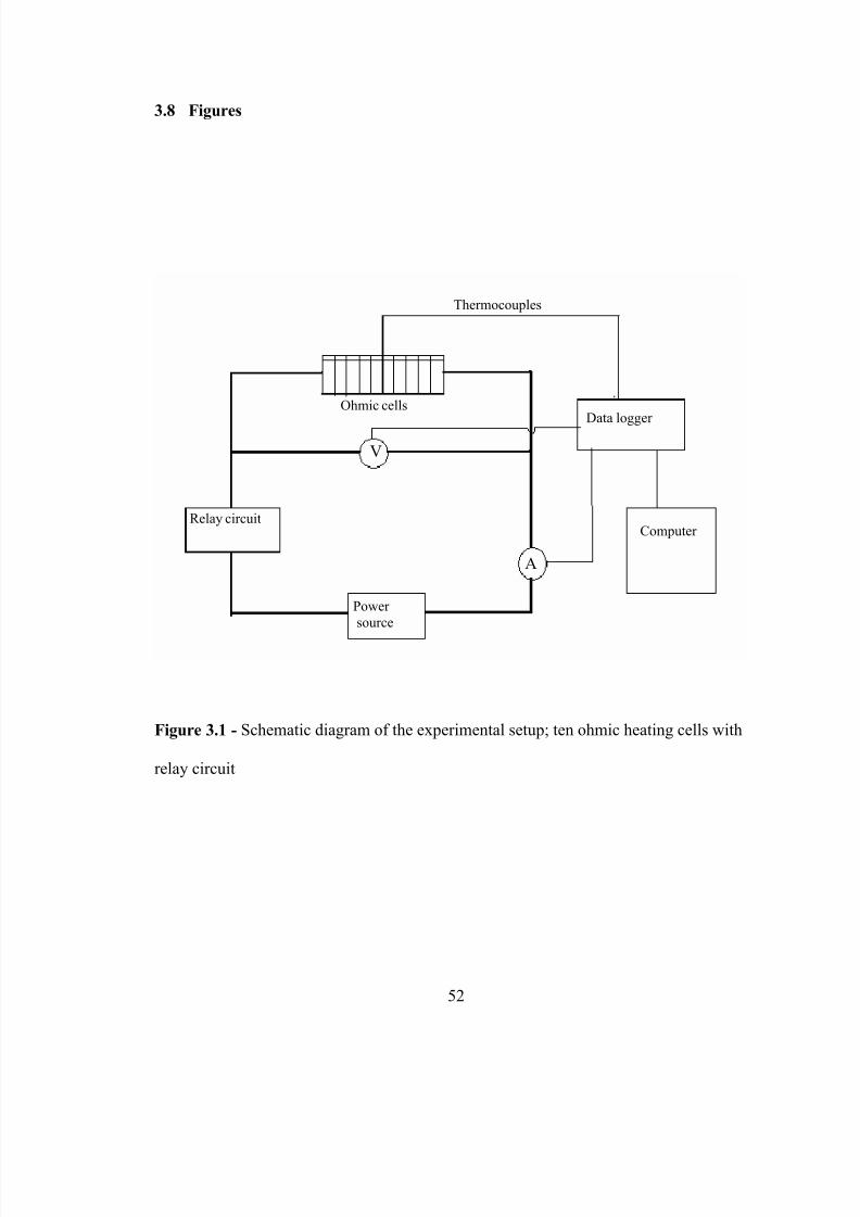
5/9/2018 Sarang Sanjay S - slidepdf.com
http://slidepdf.com/reader/full/sarang-sanjay-s 70/170
3.8 Figures
Thermocouples
Ohmic cells
V
A
Data logger
Power
source
Computer Relay circuit
Figure 3.1 - Schematic diagram of the experimental setup; ten ohmic heating cells with
relay circuit
52
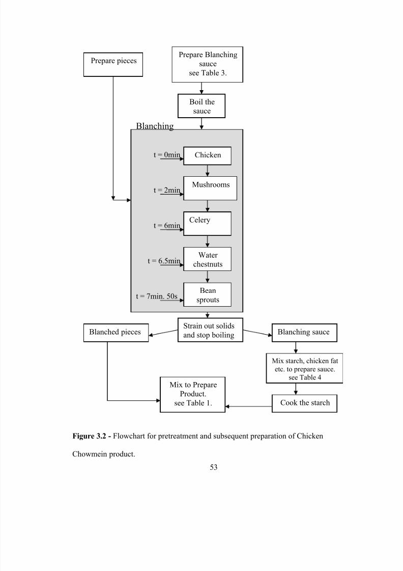
5/9/2018 Sarang Sanjay S - slidepdf.com
http://slidepdf.com/reader/full/sarang-sanjay-s 71/170
Chicken
Mushrooms
Celery
Water
chestnuts
Bean
sprouts
Prepare Blanching
sauce
see Table 3.
Prepare pieces
Boil thesauce
t = 7min. 50s
t = 6.5min
t = 6min
t = 2min
t = 0min
Blanching
Strain out solids
and stop boiling Blanching sauceBlanched pieces
Mix starch, chicken fat
etc. to prepare sauce.
see Table 4Mix to Prepare
Product.
see Table 1. Cook the starch
Figure 3.2 - Flowchart for pretreatment and subsequent preparation of Chicken
Chowmein product.
53
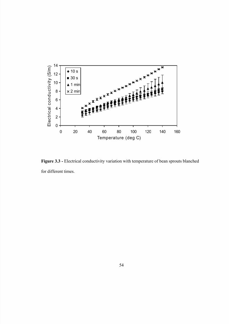
5/9/2018 Sarang Sanjay S - slidepdf.com
http://slidepdf.com/reader/full/sarang-sanjay-s 72/170
0
2
4
6
8
10
12
14
0 20 40 60 80 100 120 140 160
Temperature (deg C)
E l e c t r i c a l c o n d u c t i v i t y ( S / m )
10 s
30 s
1 min
2 min
Figure 3.3 - Electrical conductivity variation with temperature of bean sprouts blanched
for different times.
54
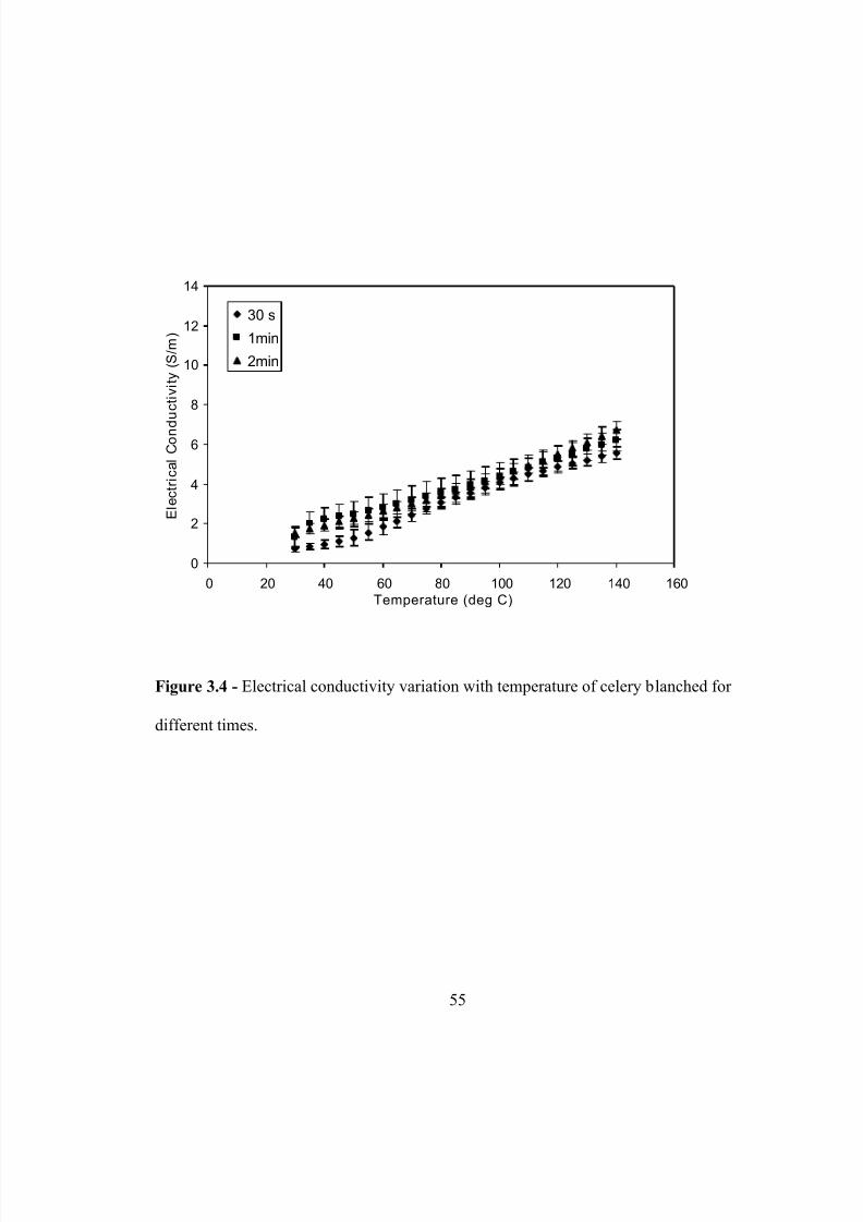
5/9/2018 Sarang Sanjay S - slidepdf.com
http://slidepdf.com/reader/full/sarang-sanjay-s 73/170
0
2
4
6
8
10
12
14
0 20 40 60 80 100 120 140 160Temperature (deg C)
E l e c t r i c a l C o n d
u c t i v i t y ( S / m )
30 s
1min
2min
Figure 3.4 - Electrical conductivity variation with temperature of celery blanched for
different times.
55
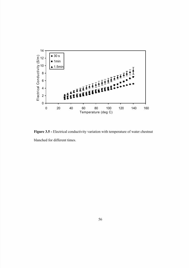
5/9/2018 Sarang Sanjay S - slidepdf.com
http://slidepdf.com/reader/full/sarang-sanjay-s 74/170
0
2
4
6
8
10
12
14
0 20 40 60 80 100 120 140 160Temperature (deg C)
E l e c t
r i c a l C o n d u c t i v i t y ( S / m ) 30 s
1min
1.5min
Figure 3.5 - Electrical conductivity variation with temperature of water chestnut
blanched for different times.
56
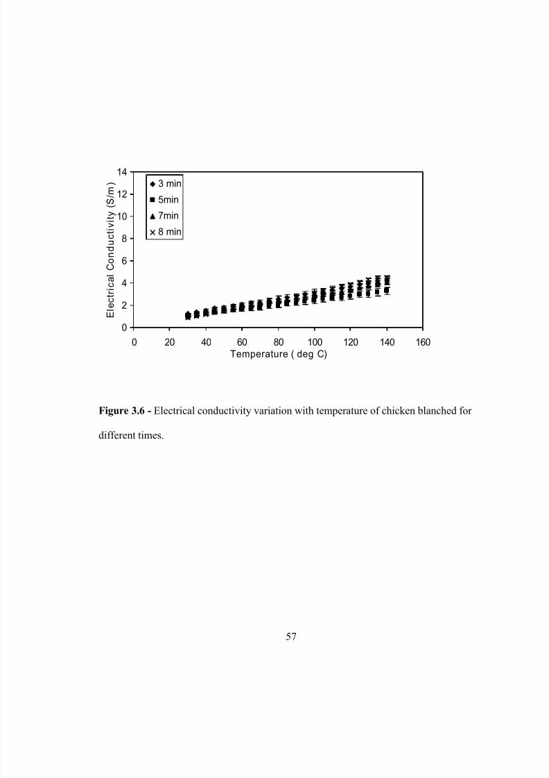
5/9/2018 Sarang Sanjay S - slidepdf.com
http://slidepdf.com/reader/full/sarang-sanjay-s 75/170
0
2
4
6
8
10
12
14
0 20 40 60 80 100 120 140 160Temperature ( deg C)
E l e c t r i c a l C o n d u c t i v i t y ( S / m ) 3 min
5min
7min
8 min
Figure 3.6 - Electrical conductivity variation with temperature of chicken blanched for
different times.
57
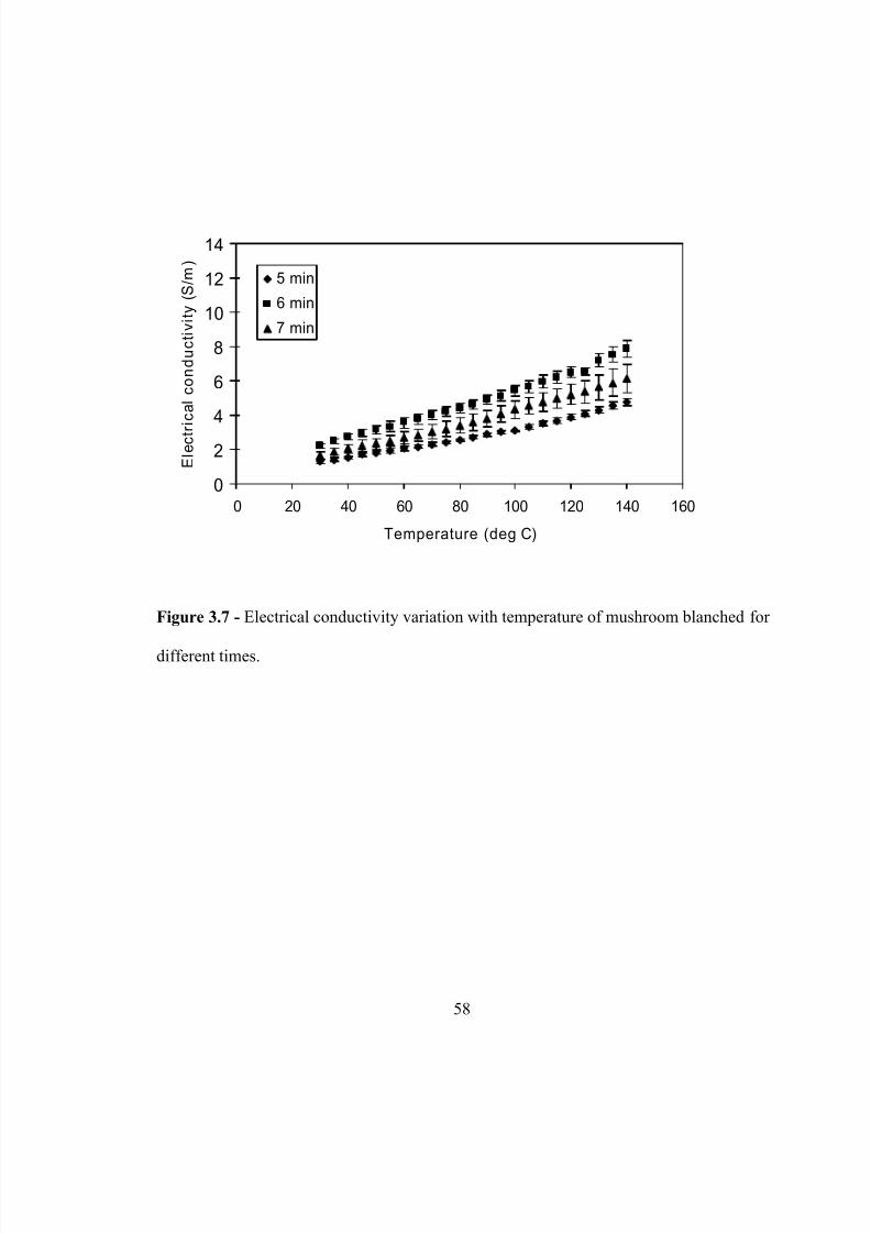
5/9/2018 Sarang Sanjay S - slidepdf.com
http://slidepdf.com/reader/full/sarang-sanjay-s 76/170
0
2
4
6
8
10
12
14
0 20 40 60 80 100 120 140 160
Temperature (deg C)
E l e c t r
i c a l c o n d u c t i v i t y ( S / m )
5 min
6 min
7 min
Figure 3.7 - Electrical conductivity variation with temperature of mushroom blanched for
different times.
58
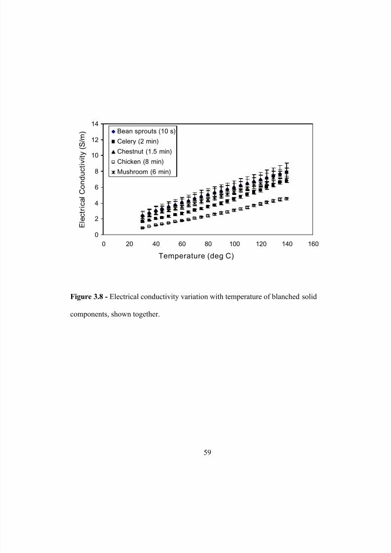
5/9/2018 Sarang Sanjay S - slidepdf.com
http://slidepdf.com/reader/full/sarang-sanjay-s 77/170
0
2
4
6
8
10
12
14
0 20 40 60 80 100 120 140 160
Temperature (deg C)
E l e c t r i c a l C
o n d u c t i v i t y ( S / m ) Bean sprouts (10 s)
Celery (2 min)
Chestnut (1.5 min)
Chicken (8 min)
Mushroom (6 min)
Figure 3.8 - Electrical conductivity variation with temperature of blanched solid
components, shown together.
59
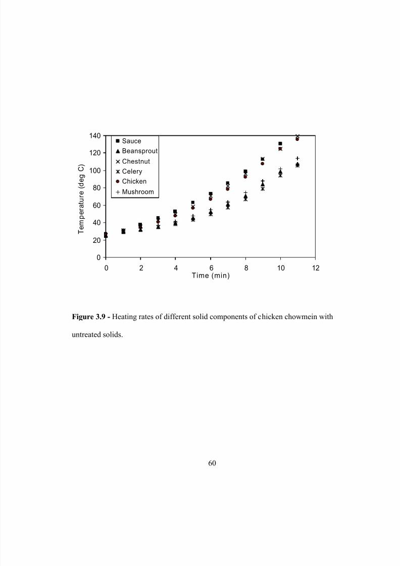
5/9/2018 Sarang Sanjay S - slidepdf.com
http://slidepdf.com/reader/full/sarang-sanjay-s 78/170
0
20
40
60
80
100
120
140
0 2 4 6 8 10 1Time (min)
T e m p e r a t u r e ( d e g C )
2
Sauce
Beansprout
Chestnut
Celery
Chicken
Mushroom
Figure 3.9 - Heating rates of different solid components of chicken chowmein with
untreated solids.
60
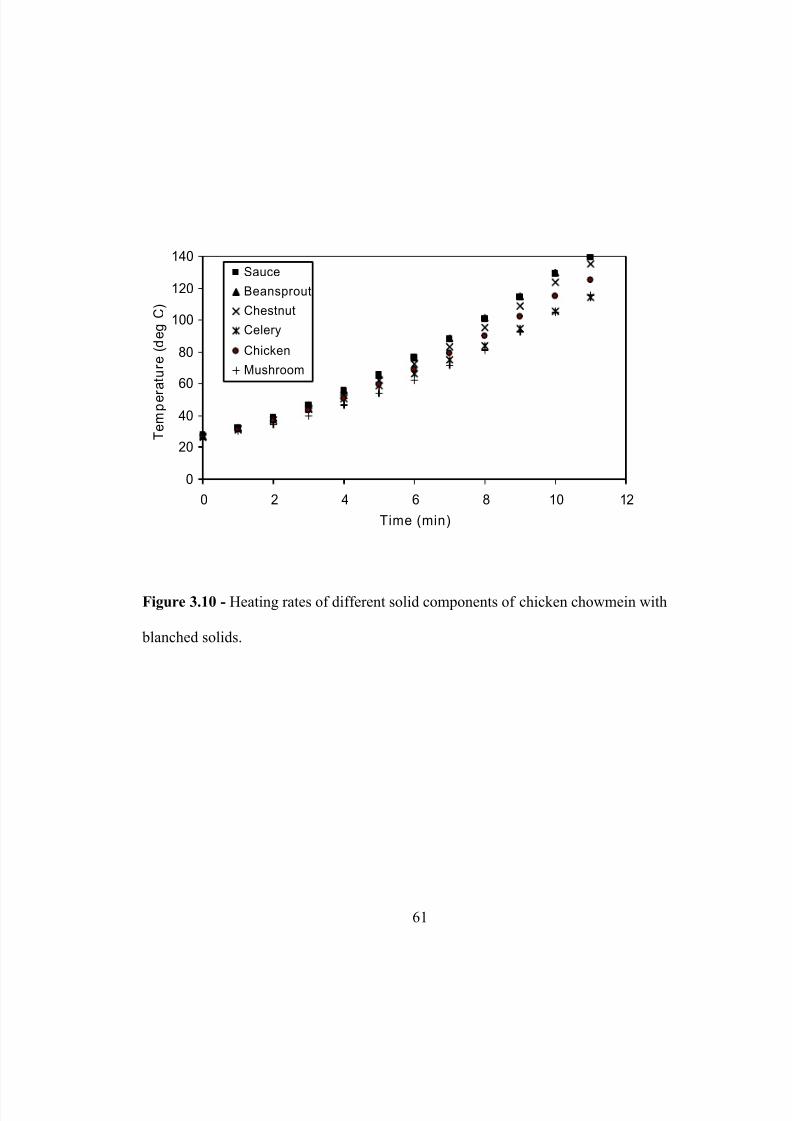
5/9/2018 Sarang Sanjay S - slidepdf.com
http://slidepdf.com/reader/full/sarang-sanjay-s 79/170
0
20
40
60
80
100
120
140
0 2 4 6 8 10 1
Time (min)
T e m p e r a t u r e ( d e g C )
2
Sauce
Beansprout
Chestnut
Celery
Chicken
Mushroom
Figure 3.10 - Heating rates of different solid components of chicken chowmein with
blanched solids.
61
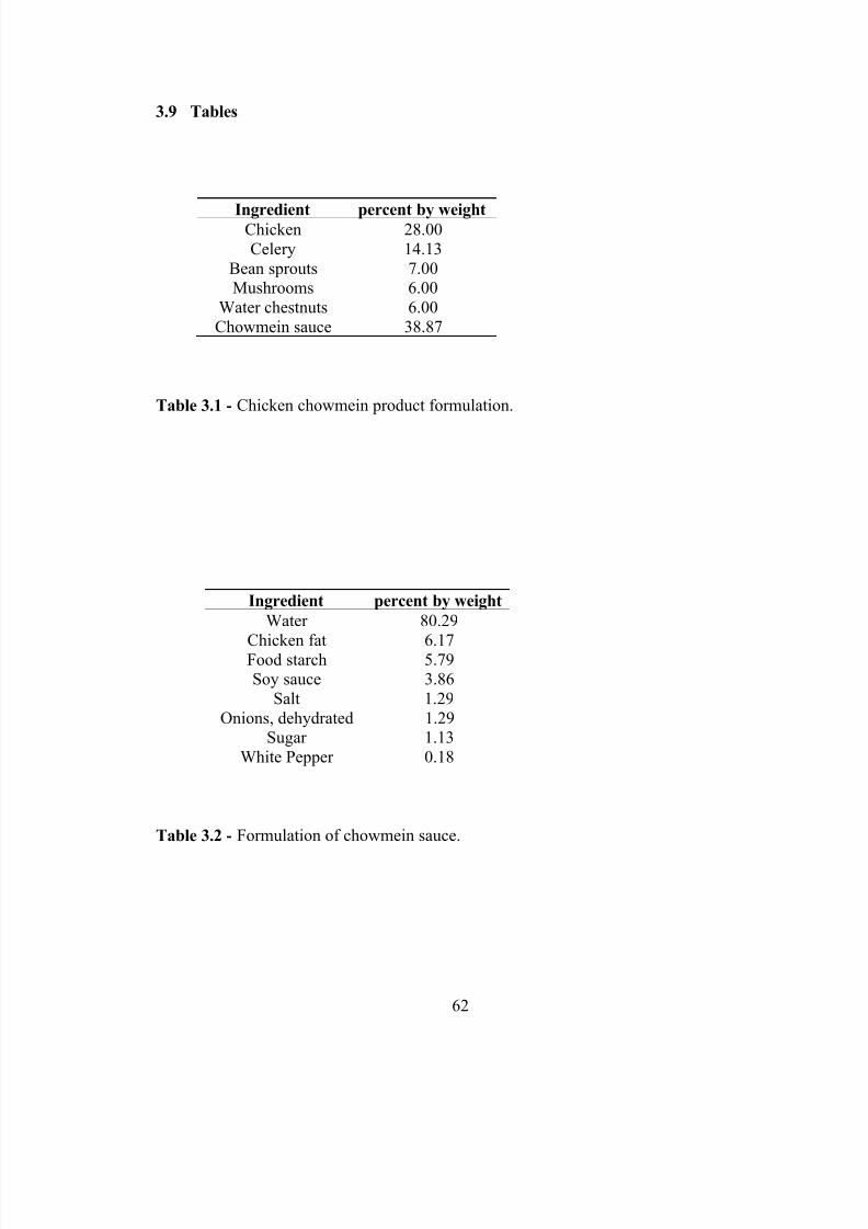
5/9/2018 Sarang Sanjay S - slidepdf.com
http://slidepdf.com/reader/full/sarang-sanjay-s 80/170
62
3.9 Tables
Ingredient percent by weightChicken 28.00
Celery 14.13
Bean sprouts 7.00Mushrooms 6.00
Water chestnuts 6.00
Chowmein sauce 38.87
Table 3.1 - Chicken chowmein product formulation.
Ingredient percent by weight
Water 80.29
Chicken fat 6.17Food starch 5.79Soy sauce 3.86
Salt 1.29
Onions, dehydrated 1.29Sugar 1.13
White Pepper 0.18
Table 3.2 - Formulation of chowmein sauce.
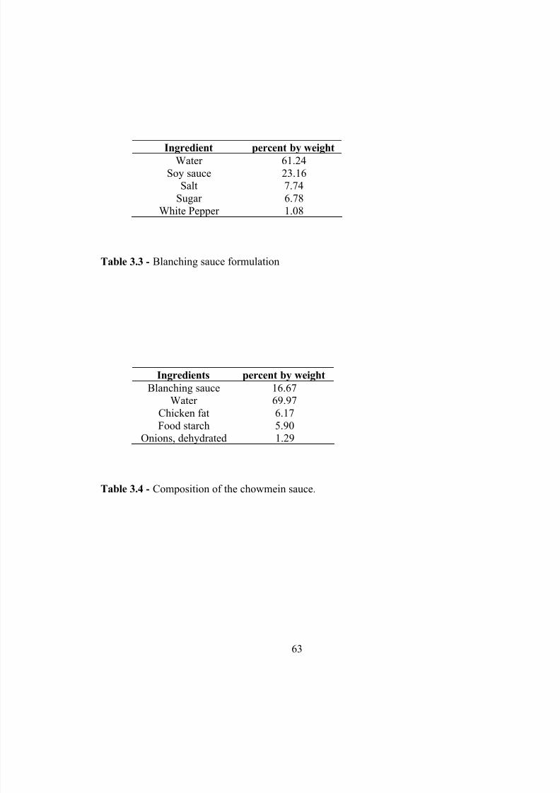
5/9/2018 Sarang Sanjay S - slidepdf.com
http://slidepdf.com/reader/full/sarang-sanjay-s 81/170
63
Ingredient percent by weight
Water 61.24
Soy sauce 23.16Salt 7.74
Sugar 6.78
White Pepper 1.08
Table 3.3 - Blanching sauce formulation
Ingredients percent by weight
Blanching sauce
16.67Water 69.97
Chicken fat 6.17Food starch 5.90
Onions, dehydrated 1.29
Table 3.4 - Composition of the chowmein sauce.
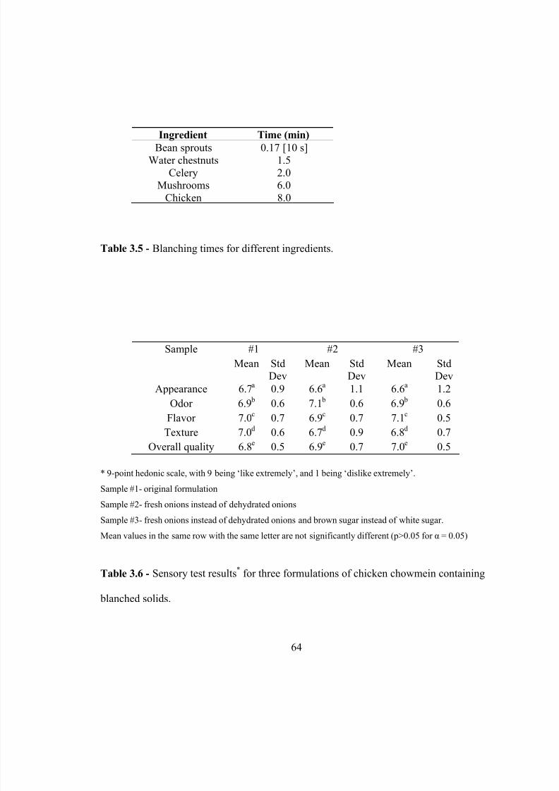
5/9/2018 Sarang Sanjay S - slidepdf.com
http://slidepdf.com/reader/full/sarang-sanjay-s 82/170
64
Ingredient Time (min)Bean sprouts 0.17 [10 s]
Water chestnuts 1.5
Celery 2.0Mushrooms 6.0
Chicken 8.0
Table 3.5 - Blanching times for different ingredients.
Sample #1 #2 #3
Mean StdDev
Mean StdDev
Mean StdDev
Appearance 6.7a
0.9 6.6a
1.1 6.6a
1.2
Odor 6.9 b
0.6 7.1 b
0.6 6.9 b
0.6
Flavor 7.0c 0.7 6.9c 0.7 7.1c 0.5
Texture 7.0d
0.6 6.7d
0.9 6.8d
0.7
Overall quality 6.8e
0.5 6.9e
0.7 7.0e
0.5
* 9-point hedonic scale, with 9 being ‘like extremely’, and 1 being ‘dislike extremely’.
Sample #1- original formulation
Sample #2- fresh onions instead of dehydrated onions
Sample #3- fresh onions instead of dehydrated onions and brown sugar instead of white sugar.
Mean values in the same row with the same letter are not significantly different (p>0.05 for α = 0.05)
Table 3.6 - Sensory test results*
for three formulations of chicken chowmein containing
blanched solids.
5/9/2018 Sarang Sanjay S - slidepdf.com
http://slidepdf.com/reader/full/sarang-sanjay-s 83/170
65
CHAPTER 4
SALT DIFFUSION INTO VEGETABLE TISSUE AS A PRETREATMENT FOR
OHMIC HEATING
4.1 Abstract
The apparent diffusion coefficient and equilibrium distribution coefficient of
sodium chloride in Chinese water chestnut were determined for salt solution
concentrations between 5 and 10% and at temperatures in the range 25-80oC.
Equilibrium distribution coefficient values were close to 1.0 and did not depend on salt
concentration or temperature. The apparent diffusion coefficient of salt in water chestnut
is not dependent on the concentration of the salt solution and significantly increased with
temperature (P = 0.001) following the Arrhenius equation. Computational fluid dynamic
software was used to determine salt concentration and electrical conductivity profile after
blanching pretreatment and heating profile of pretreated water chestnut disc under static
ohmic heating condition. After blanching, though concentration and electrical
conductivity is not uniformly distributed throughout the solid, it was possible to increase
the overall electrical conductivity and heat the solid more rapidly during ohmic heating.
5/9/2018 Sarang Sanjay S - slidepdf.com
http://slidepdf.com/reader/full/sarang-sanjay-s 84/170
66
4.2 Introduction
Ohmic or electrical resistance heating involves the application of a cyclical
potential to a material, resulting in heat generation due to ionic motion. Ohmic heating
has potential applications in the food industry for processing of liquid-solid food
mixtures, also termed particulate foods (Palaniappan & Sastry, 2002). In an ohmic
heating process for particulate foods, the most desirable situation is that in which the
electrical conductivities of fluid and solid particles are equal (Wang & Sastry, 1993 a).
Palaniappan & Sastry (1991), and Mitchell & de Alwis (1989) measured electrical
conductivity of some solid foods. Ruhlman, Jin & Zhang (2001) reported electrical
conductivity of some liquid foods at different temperatures. For particulate foods it can
be observed that most vegetables and meats have lower electrical conductivities than
liquids. It is possible to increase the electrolytic content within foodstuffs, and raise
electrical conductivity by salt infusion via soaking or blanching of solids in salt solution.
This may be used as a pretreatment for ohmic heating for particulate foods to obtain more
uniform heat treatment, if the composition and other properties of the food are not greatly
affected (Palaniappan & Sastry, 1991; Wang & Sastry, 1993 a).
Diffusion of salt in solid foods such as pork, beef and fish has been studied by
many researchers (Wistreich, Morse & Kenyon, 1960; Wood, 1966; Del Valle &
Nickerson, 1967a, b; Dussap & Gros, 1980). Liu (1992) determined the apparent
diffusion coefficient of salt in potato tissue in different sodium chloride concentrations
(1-5% w/v) and at temperature between 50oC and 120
oC. Drusas & Vagenas (1988)
studied salt diffusion in green olives at 20oC and 7-16% w/v salt solutions. Wang &
Sastry (1993 b) determined salt diffusivity in potato tissue at 25oC and 1-3% w/v salt
5/9/2018 Sarang Sanjay S - slidepdf.com
http://slidepdf.com/reader/full/sarang-sanjay-s 85/170
67
solutions. These researchers studied salt diffusion by soaking vegetable pieces in salt
solution at different temperatures and determining the salt uptake by the tissues. This
method is time consuming, and it is difficult to determine salt concentration in vegetable
tissue. Moreover, diffusion studies were generally made in either lower salt concentration
solutions or at lower temperatures. A quicker, simpler, yet accurate method is needed.
For this study we have focused on Chinese water chestnut (CWC), an ingredient
in the military’s chicken chowmein formulation, which is currently being investigated for
processing by ohmic heating. The methodology could, however be used for any vegetable
tissue. CWC is the corm of the sedge that grows in damp conditions. The dark-brown
corms are peeled before cooking or canning. The bulk of the edible region consists of
starch-rich, thin walled storage parenchyma similar in appearance to potato, interspersed
with vascular strands. However, in contrast to potato, CWC is notable for its ability to
maintain a firm and crunchy texture after considerable heat treatment during canning or
cooking (Parker & Waldron, 1995; Mudahar & Jen, 1991; Parker, C. C., Parker, M. L.,
Smith & Waldron, 2003). CWC is commonly used in oriental foods and is prized for its
crispiness.
The objectives of this study were; to develop a simple method to measure salt
diffusion into vegetable tissue, and to investigate diffusion of salt into water chestnut
tissue under different levels of sodium chloride concentration (5, 7.5 and 10% w/v) and
temperature (25 – 80
o
C). Higher salt concentration and temperature may reduce the
pretreatment time necessary for ohmic heat processing. The diffusion data obtained was
used further to solve mass transfer problem, using a Computational Fluid Dynamics
(CFD) software package, to predict salt concentration profile in water chestnut disc.
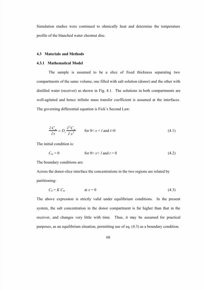
5/9/2018 Sarang Sanjay S - slidepdf.com
http://slidepdf.com/reader/full/sarang-sanjay-s 86/170
Simulation studies were continued to ohmically heat and determine the temperature
profile of the blanched water chestnut disc.
4.3 Materials and Methods
4.3.1 Mathematical Model
The sample is assumed to be a slice of fixed thickness separating two
compartments of the same volume, one filled with salt solution (donor) and the other with
distilled water (receiver) as shown in Fig. 4.1. The solutions in both compartments are
well-agitated and hence infinite mass transfer coefficient is assumed at the interfaces.
The governing differential equation is Fick’s Second Law:
2
2
x
C D
t
C m s
m
∂
∂=
∂
∂for 0< x < l and t >0 (4.1)
The initial condition is:
C m = 0 for 0< x< l and t = 0 (4.2)
The boundary conditions are:
Across the donor-slice interface the concentrations in the two regions are related by
partitioning:
C d = K C m at x = 0 (4.3)
The above expression is strictly valid under equilibrium conditions. In the present
system, the salt concentration in the donor compartment is far higher than that in the
receiver, and changes very little with time. Thus, it may be assumed for practical
purposes, as an equilibrium situation, permitting use of eq. (4.3) as a boundary condition.
68
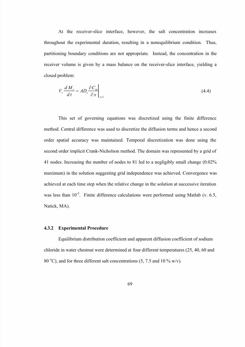
5/9/2018 Sarang Sanjay S - slidepdf.com
http://slidepdf.com/reader/full/sarang-sanjay-s 87/170
At the receiver-slice interface, however, the salt concentration increases
throughout the experimental duration, resulting in a nonequilibrium condition. Thus,
partitioning boundary conditions are not appropriate. Instead, the concentration in the
receiver volume is given by a mass balance on the receiver-slice interface, yielding a
closed problem:
l x
m s
ir
x
C AD
t d
M d V
=∂
∂= (4.4)
This set of governing equations was discretized using the finite difference
method. Central difference was used to discretize the diffusion terms and hence a second
order spatial accuracy was maintained. Temporal discretization was done using the
second order implicit Crank-Nicholson method. The domain was represented by a grid of
41 nodes. Increasing the number of nodes to 81 led to a negligibly small change (0.02%
maximum) in the solution suggesting grid independence was achieved. Convergence was
achieved at each time step when the relative change in the solution at successive iteration
was less than 10-5
. Finite difference calculations were performed using Matlab (v. 6.5,
Natick, MA).
4.3.2 Experimental Procedure
Equilibrium distribution coefficient and apparent diffusion coefficient of sodium
chloride in water chestnut were determined at four different temperatures (25, 40, 60 and
80oC), and for three different salt concentrations (5, 7.5 and 10 % w/v).
69
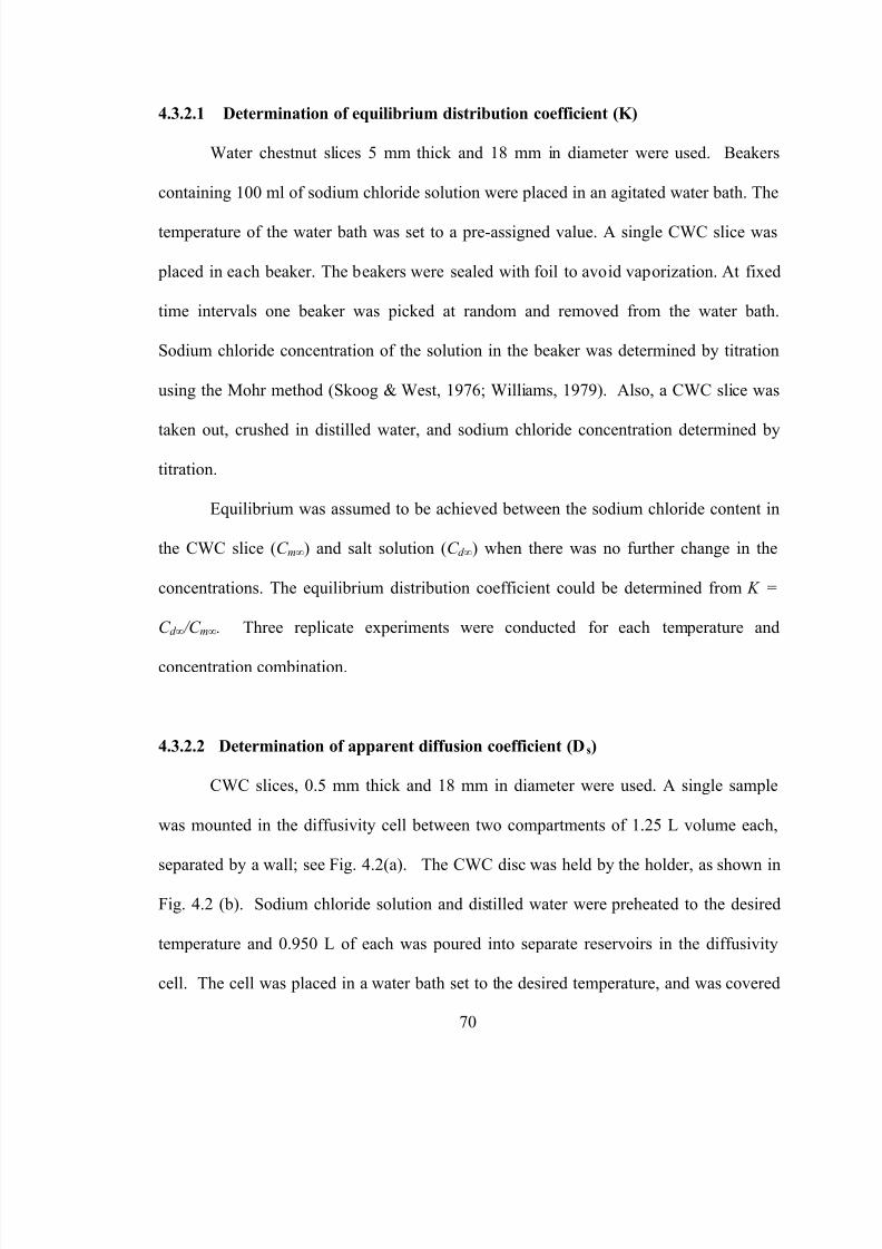
5/9/2018 Sarang Sanjay S - slidepdf.com
http://slidepdf.com/reader/full/sarang-sanjay-s 88/170
70
4.3.2.1 Determination of equilibrium distribution coefficient (K)
Water chestnut slices 5 mm thick and 18 mm in diameter were used. Beakers
containing 100 ml of sodium chloride solution were placed in an agitated water bath. The
temperature of the water bath was set to a pre-assigned value. A single CWC slice was
placed in each beaker. The beakers were sealed with foil to avoid vaporization. At fixed
time intervals one beaker was picked at random and removed from the water bath.
Sodium chloride concentration of the solution in the beaker was determined by titration
using the Mohr method (Skoog & West, 1976; Williams, 1979). Also, a CWC slice was
taken out, crushed in distilled water, and sodium chloride concentration determined by
titration.
Equilibrium was assumed to be achieved between the sodium chloride content in
the CWC slice (C m∞) and salt solution (C d ∞) when there was no further change in the
concentrations. The equilibrium distribution coefficient could be determined from K =
C d ∞ /C m∞. Three replicate experiments were conducted for each temperature and
concentration combination.
4.3.2.2 Determination of apparent diffusion coefficient (Ds)
CWC slices, 0.5 mm thick and 18 mm in diameter were used. A single sample
was mounted in the diffusivity cell between two compartments of 1.25 L volume each,
separated by a wall; see Fig. 4.2(a). The CWC disc was held by the holder, as shown in
Fig. 4.2 (b). Sodium chloride solution and distilled water were preheated to the desired
temperature and 0.950 L of each was poured into separate reservoirs in the diffusivity
cell. The cell was placed in a water bath set to the desired temperature, and was covered
5/9/2018 Sarang Sanjay S - slidepdf.com
http://slidepdf.com/reader/full/sarang-sanjay-s 89/170
with foil to prevent evaporation. The temperature of the solutions was controlled within
±2oC of the pre-assigned temperatures. The solutions in both compartments were
continuously stirred to ensure mass transfer coefficient at the interfaces were very high.
Sodium chloride diffuses through CWC and enters the receiver region. At fixed time
intervals, 5 ml solution from the receiver was withdrawn and the salt concentration was
determined by titration. As 5 ml solution was withdrawn every time from the receiver
compartment, the receiver volume changes during the experiment. The maximum volume
change for the length of the experiment was about 4% and was not accounted for. Two
replicate experiments were conducted for each temperature and concentration
combination.
The apparent diffusion coefficient (Ds) was estimated using the least squares
method to minimize the difference between the measured and predicted receiver salt
concentration:
2
1
)( i
N
i
i M C S ∑=
−= (4.5)
4.3.3 Statistical Analysis
Equilibrium distribution coefficient and apparent diffusion coefficient data were
subjected to analysis of variance (ANOVA).
4.3.4 Computational Simulation
4.3.4.1 Blanching
Simulation studies were performed for the 3D case. The sample was assumed to
be a water chestnut disc of 7.5 x 10⁻³
m in thickness and 1.8 x 10⁻²
m in diameter. The
71
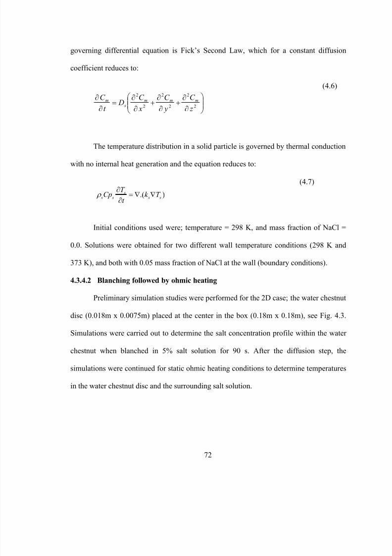
5/9/2018 Sarang Sanjay S - slidepdf.com
http://slidepdf.com/reader/full/sarang-sanjay-s 90/170
governing differential equation is Fick’s Second Law, which for a constant diffusion
coefficient reduces to:
⎟⎟ ⎞
⎜⎜⎛
∂∂+
∂∂+
∂∂=
∂∂
2
2
2
2
2
2 C C C DC mmm s
m
⎠⎝ z y xt
(4.6)
The temperature distribution in a solid particle is governed by thermal conduction
with no internal heat generation and the equation reduces to:
.( ) s s s s
T Cp k T t
ρ ∂
= ∇ ∇∂ s
(4.7)
Initial conditions used were; temperature = 298 K, and mass fraction of NaCl =
0.0. Solutions were obtained for two different wall temperature conditions (298 K and
373 K), and both with 0.05 mass fraction of NaCl at the wall (boundary conditions).
4.3.4.2 Blanching followed by ohmic heating
Preliminary simulation studies were performed for the 2D case; the water chestnut
disc (0.018m x 0.0075m) placed at the center in the box (0.18m x 0.18m), see Fig. 4.3.
Simulations were carried out to determine the salt concentration profile within the water
chestnut when blanched in 5% salt solution for 90 s. After the diffusion step, the
simulations were continued for static ohmic heating conditions to determine temperatures
in the water chestnut disc and the surrounding salt solution.
72
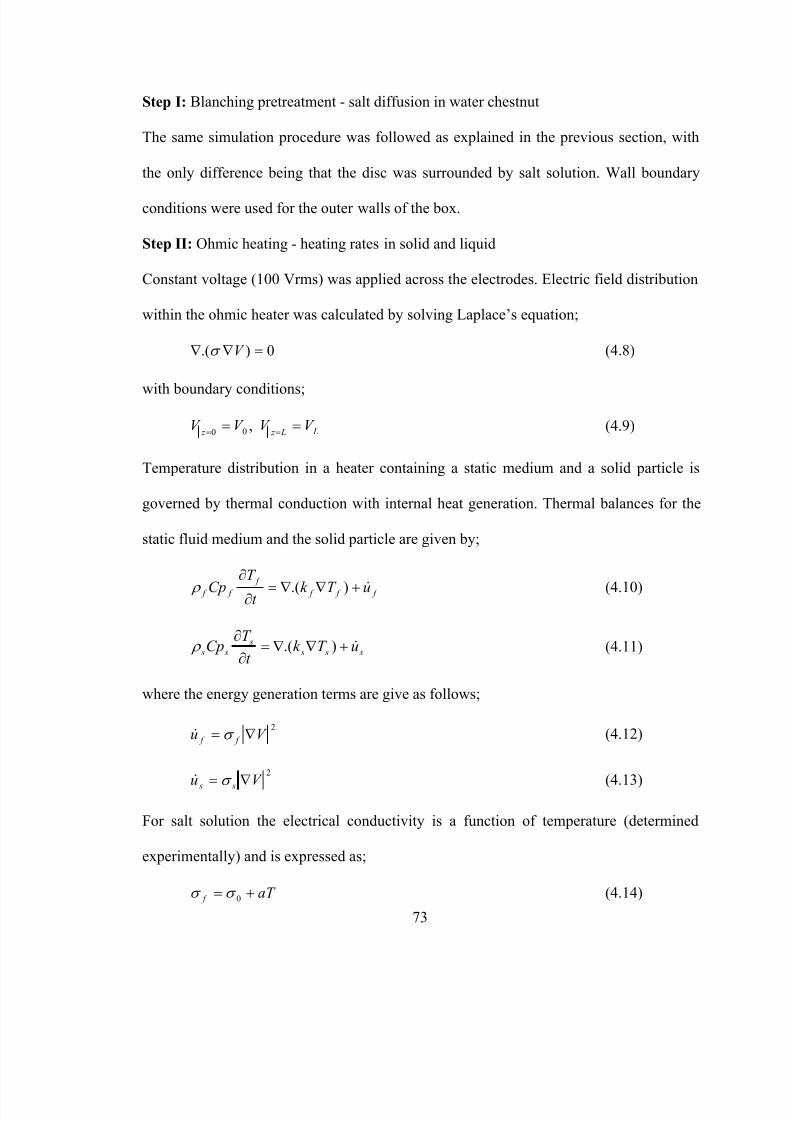
5/9/2018 Sarang Sanjay S - slidepdf.com
http://slidepdf.com/reader/full/sarang-sanjay-s 91/170
Step I: Blanching pretreatment - salt diffusion in water chestnut
The same simulation procedure was followed as explained in the previous section, with
the only difference being that the disc was surrounded by salt solution. Wall boundary
conditions were used for the outer walls of the box.
Step II: Ohmic heating - heating rates in solid and liquid
Constant voltage (100 Vrms) was applied across the electrodes. Electric field distribution
within the ohmic heater was calculated by solving Laplace’s equation;
0).( =∇∇ V σ (4.8)
with boundary conditions;
L L z z V V V V == ==
,00(4.9)
Temperature distribution in a heater containing a static medium and a solid particle is
governed by thermal conduction with internal heat generation. Thermal balances for the
static fluid medium and the solid particle are given by;
f f f
f
f f uT k t
T
Cp &+∇∇=∂
∂).( ρ (4.10)
s s s s
s s uT k t
T Cp &+∇∇=
∂
∂).( ρ (4.11)
where the energy generation terms are give as follows;
2V u f f ∇= σ & (4.12)
2
V u s s∇= σ
& (4.13)
For salt solution the electrical conductivity is a function of temperature (determined
experimentally) and is expressed as;
aT f += 0σ σ (4.14)
73
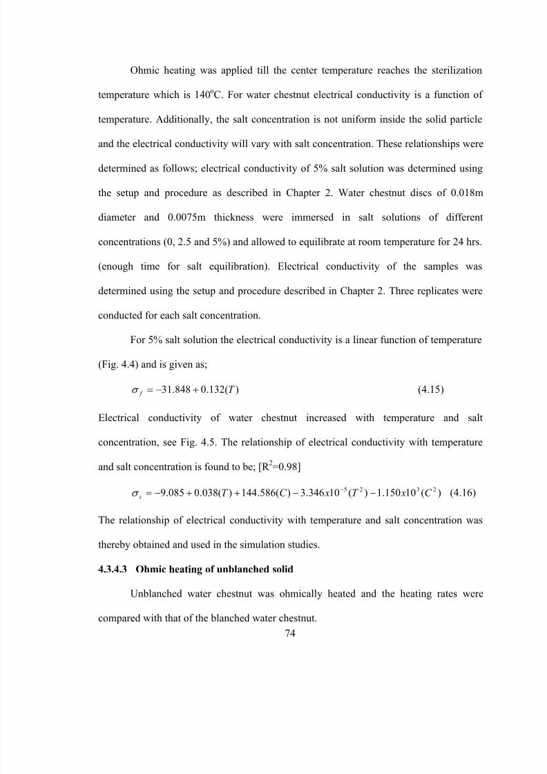
5/9/2018 Sarang Sanjay S - slidepdf.com
http://slidepdf.com/reader/full/sarang-sanjay-s 92/170
Ohmic heating was applied till the center temperature reaches the sterilization
temperature which is 140oC. For water chestnut electrical conductivity is a function of
temperature. Additionally, the salt concentration is not uniform inside the solid particle
and the electrical conductivity will vary with salt concentration. These relationships were
determined as follows; electrical conductivity of 5% salt solution was determined using
the setup and procedure as described in Chapter 2. Water chestnut discs of 0.018m
diameter and 0.0075m thickness were immersed in salt solutions of different
concentrations (0, 2.5 and 5%) and allowed to equilibrate at room temperature for 24 hrs.
(enough time for salt equilibration). Electrical conductivity of the samples was
determined using the setup and procedure described in Chapter 2. Three replicates were
conducted for each salt concentration.
For 5% salt solution the electrical conductivity is a linear function of temperature
(Fig. 4.4) and is given as;
)(132.0848.31 T f +−=σ (4.15)
Electrical conductivity of water chestnut increased with temperature and salt
concentration, see Fig. 4.5. The relationship of electrical conductivity with temperature
and salt concentration is found to be; [R 2=0.98]
(4.16))(10150.1)(10346.3)(586.144)(038.0085.9 2325 C xT xC T s −−++−= −σ
The relationship of electrical conductivity with temperature and salt concentration was
thereby obtained and used in the simulation studies.
4.3.4.3 Ohmic heating of unblanched solid
Unblanched water chestnut was ohmically heated and the heating rates were
compared with that of the blanched water chestnut.
74
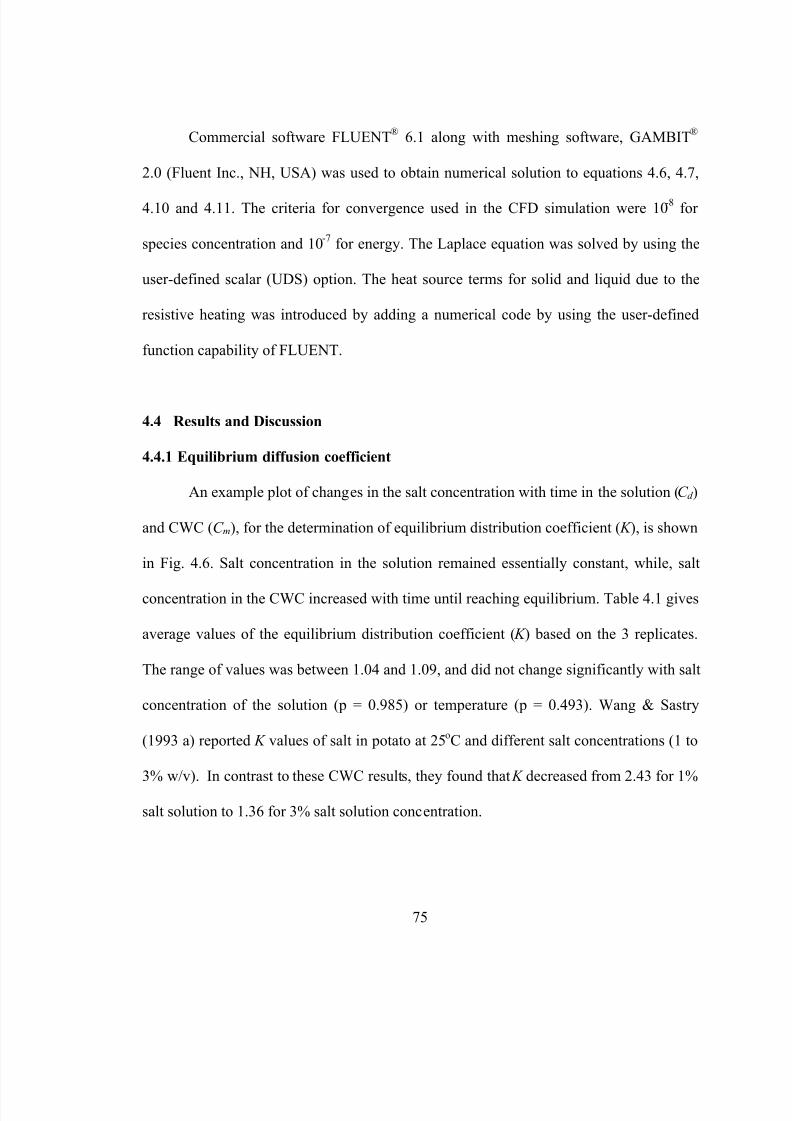
5/9/2018 Sarang Sanjay S - slidepdf.com
http://slidepdf.com/reader/full/sarang-sanjay-s 93/170
75
Commercial software FLUENT®
6.1 along with meshing software, GAMBIT®
2.0 (Fluent Inc., NH, USA) was used to obtain numerical solution to equations 4.6, 4.7,
4.10 and 4.11. The criteria for convergence used in the CFD simulation were 10-8
for
species concentration and 10-7
for energy. The Laplace equation was solved by using the
user-defined scalar (UDS) option. The heat source terms for solid and liquid due to the
resistive heating was introduced by adding a numerical code by using the user-defined
function capability of FLUENT.
4.4 Results and Discussion
4.4.1 Equilibrium diffusion coefficient
An example plot of changes in the salt concentration with time in the solution (C d )
and CWC (C m), for the determination of equilibrium distribution coefficient ( K ), is shown
in Fig. 4.6. Salt concentration in the solution remained essentially constant, while, salt
concentration in the CWC increased with time until reaching equilibrium. Table 4.1 gives
average values of the equilibrium distribution coefficient ( K ) based on the 3 replicates.
The range of values was between 1.04 and 1.09, and did not change significantly with salt
concentration of the solution (p = 0.985) or temperature (p = 0.493). Wang & Sastry
(1993 a) reported K values of salt in potato at 25oC and different salt concentrations (1 to
3% w/v). In contrast to these CWC results, they found that K decreased from 2.43 for 1%
salt solution to 1.36 for 3% salt solution concentration.
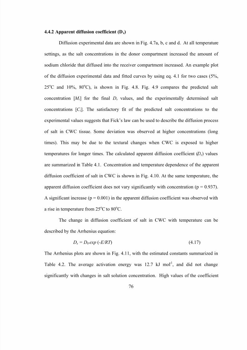
5/9/2018 Sarang Sanjay S - slidepdf.com
http://slidepdf.com/reader/full/sarang-sanjay-s 94/170
76
4.4.2 Apparent diffusion coefficient (Ds)
Diffusion experimental data are shown in Fig. 4.7a, b, c and d. At all temperature
settings, as the salt concentrations in the donor compartment increased the amount of
sodium chloride that diffused into the receiver compartment increased. An example plot
of the diffusion experimental data and fitted curves by using eq. 4.1 for two cases (5%,
25oC and 10%, 80
oC), is shown in Fig. 4.8. Fig. 4.9 compares the predicted salt
concentration [M i] for the final D s values, and the experimentally determined salt
concentrations [C i]. The satisfactory fit of the predicted salt concentrations to the
experimental values suggests that Fick’s law can be used to describe the diffusion process
of salt in CWC tissue. Some deviation was observed at higher concentrations (long
times). This may be due to the textural changes when CWC is exposed to higher
temperatures for longer times. The calculated apparent diffusion coefficient ( D s) values
are summarized in Table 4.1. Concentration and temperature dependence of the apparent
diffusion coefficient of salt in CWC is shown in Fig. 4.10. At the same temperature, the
apparent diffusion coefficient does not vary significantly with concentration (p = 0.937).
A significant increase (p = 0.001) in the apparent diffusion coefficient was observed with
a rise in temperature from 25oC
to 80
oC.
The change in diffusion coefficient of salt in CWC with temperature can be
described by the Arrhenius equation:
D s = D0 exp (-E/RT ) (4.17)
The Arrhenius plots are shown in Fig. 4.11, with the estimated constants summarized in
Table 4.2. The average activation energy was 12.7 kJ mol-1
, and did not change
significantly with changes in salt solution concentration. High values of the coefficient
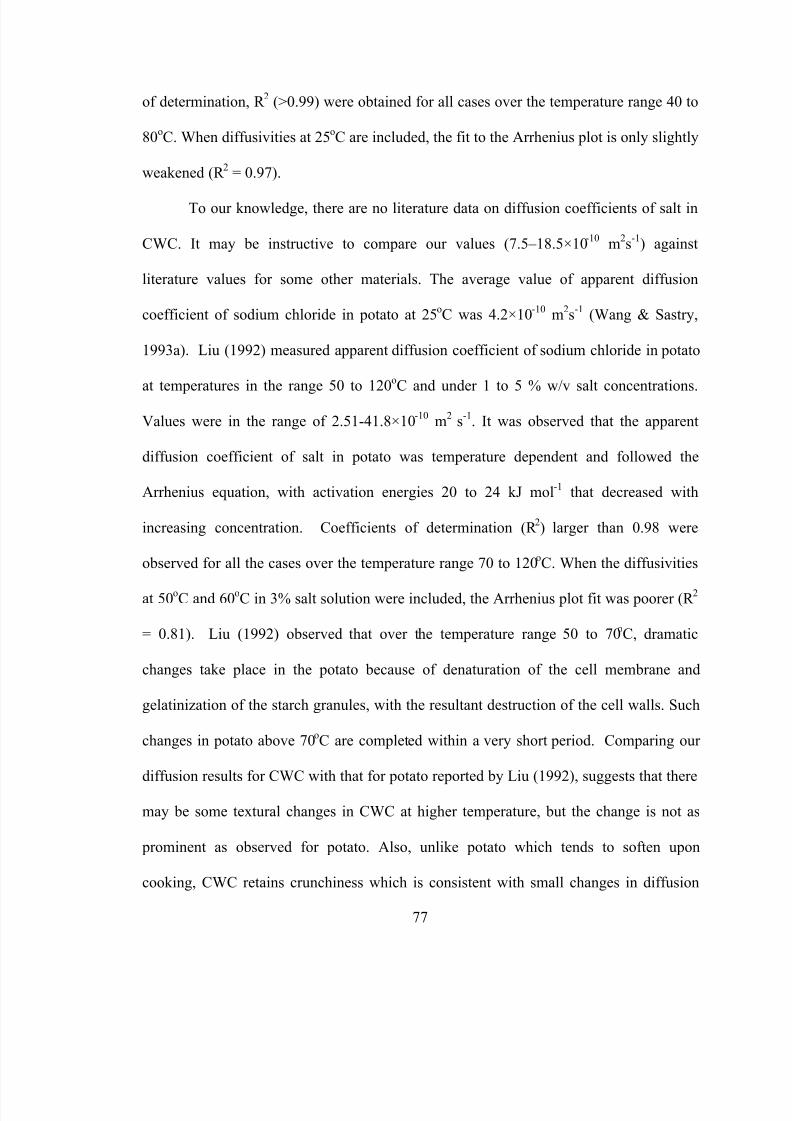
5/9/2018 Sarang Sanjay S - slidepdf.com
http://slidepdf.com/reader/full/sarang-sanjay-s 95/170
77
of determination, R 2
(>0.99) were obtained for all cases over the temperature range 40 to
80oC. When diffusivities at 25
oC are included, the fit to the Arrhenius plot is only slightly
weakened (R 2
= 0.97).
To our knowledge, there are no literature data on diffusion coefficients of salt in
CWC. It may be instructive to compare our values (7.5–18.5×10⁻¹⁰
m2s
-1) against
literature values for some other materials. The average value of apparent diffusion
coefficient of sodium chloride in potato at 25oC was 4.2×10
-10m
2s
-1(Wang & Sastry,
1993a). Liu (1992) measured apparent diffusion coefficient of sodium chloride in potato
at temperatures in the range 50 to 120
o
C and under 1 to 5 % w/v salt concentrations.
Values were in the range of 2.51-41.8×10⁻¹⁰
m2
s-1
. It was observed that the apparent
diffusion coefficient of salt in potato was temperature dependent and followed the
Arrhenius equation, with activation energies 20 to 24 kJ mol-1
that decreased with
increasing concentration. Coefficients of determination (R 2) larger than 0.98 were
observed for all the cases over the temperature range 70 to 120oC. When the diffusivities
at 50oC and 60
oC in 3% salt solution were included, the Arrhenius plot fit was poorer (R
2
= 0.81). Liu (1992) observed that over the temperature range 50 to 70oC, dramatic
changes take place in the potato because of denaturation of the cell membrane and
gelatinization of the starch granules, with the resultant destruction of the cell walls. Such
changes in potato above 70oC are completed within a very short period. Comparing our
diffusion results for CWC with that for potato reported by Liu (1992), suggests that there
may be some textural changes in CWC at higher temperature, but the change is not as
prominent as observed for potato. Also, unlike potato which tends to soften upon
cooking, CWC retains crunchiness which is consistent with small changes in diffusion
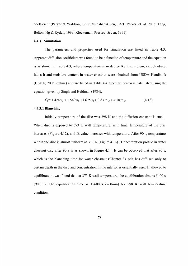
5/9/2018 Sarang Sanjay S - slidepdf.com
http://slidepdf.com/reader/full/sarang-sanjay-s 96/170
78
coefficient (Parker & Waldron, 1995; Mudahar & Jen, 1991; Parker, et. al. 2003, Tang,
Belton, Ng & Ryden, 1999; Klockeman, Pressey, & Jen, 1991).
4.4.3 Simulation
The parameters and properties used for simulation are listed in Table 4.3.
Apparent diffusion coefficient was found to be a function of temperature and the equation
is as shown in Table 4.3, where temperature is in degree Kelvin. Protein, carbohydrate,
fat, ash and moisture content in water chestnut were obtained from USDA Handbook
(USDA, 2005, online) and are listed in Table 4.4. Specific heat was calculated using the
equation given by Singh and Heldman (1984);
C p= 1.424mc + 1.549m p +1.675m f + 0.837ma + 4.187mm (4.18)
4.4.3.1 Blanching
Initially temperature of the disc was 298 K and the diffusion constant is small.
When disc is exposed to 373 K wall temperature, with time, temperature of the disc
increases (Figure 4.12), and Ds value increases with temperature. After 90 s, temperature
within the disc is almost uniform at 373 K (Figure 4.13). Concentration profile in water
chestnut disc after 90 s is as shown in Figure 4.14. It can be observed that after 90 s,
which is the blanching time for water chestnut (Chapter 3), salt has diffused only to
certain depth in the disc and concentration in the interior is essentially zero. If allowed to
equilibrate, it was found that, at 373 K wall temperature, the equilibration time is 5400 s
(90min). The equilibration time is 15600 s (260min) for 298 K wall temperature
condition.
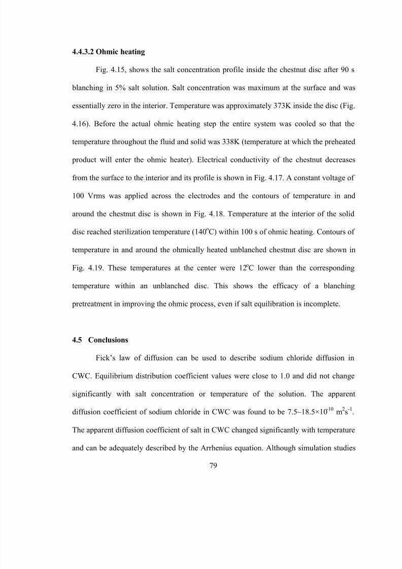
5/9/2018 Sarang Sanjay S - slidepdf.com
http://slidepdf.com/reader/full/sarang-sanjay-s 97/170
79
4.4.3.2 Ohmic heating
Fig. 4.15, shows the salt concentration profile inside the chestnut disc after 90 s
blanching in 5% salt solution. Salt concentration was maximum at the surface and was
essentially zero in the interior. Temperature was approximately 373K inside the disc (Fig.
4.16). Before the actual ohmic heating step the entire system was cooled so that the
temperature throughout the fluid and solid was 338K (temperature at which the preheated
product will enter the ohmic heater). Electrical conductivity of the chestnut decreases
from the surface to the interior and its profile is shown in Fig. 4.17. A constant voltage of
100 Vrms was applied across the electrodes and the contours of temperature in and
around the chestnut disc is shown in Fig. 4.18. Temperature at the interior of the solid
disc reached sterilization temperature (140oC) within 100 s of ohmic heating. Contours of
temperature in and around the ohmically heated unblanched chestnut disc are shown in
Fig. 4.19. These temperatures at the center were 12oC lower than the corresponding
temperature within an unblanched disc. This shows the efficacy of a blanching
pretreatment in improving the ohmic process, even if salt equilibration is incomplete.
4.5 Conclusions
Fick’s law of diffusion can be used to describe sodium chloride diffusion in
CWC. Equilibrium distribution coefficient values were close to 1.0 and did not change
significantly with salt concentration or temperature of the solution. The apparent
diffusion coefficient of sodium chloride in CWC was found to be 7.5–18.5×10⁻¹⁰
m2s
-1.
The apparent diffusion coefficient of salt in CWC changed significantly with temperature
and can be adequately described by the Arrhenius equation. Although simulation studies
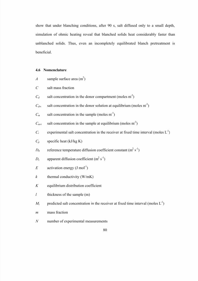
5/9/2018 Sarang Sanjay S - slidepdf.com
http://slidepdf.com/reader/full/sarang-sanjay-s 98/170
80
show that under blanching conditions, after 90 s, salt diffused only to a small depth,
simulation of ohmic heating reveal that blanched solids heat considerably faster than
unblanched solids. Thus, even an incompletely equilibrated blanch pretreatment is
beneficial.
4.6 Nomenclature
A sample surface area (m2)
C salt mass fraction
C d salt concentration in the donor compartment (moles m
-3
)
C d ∞ salt concentration in the donor solution at equilibrium (moles m-3
)
C m salt concentration in the sample (moles m-3
)
C m∞ salt concentration in the sample at equilibrium (moles m-3
)
C i experimental salt concentration in the receiver at fixed time interval (moles L-1
)
C p specific heat (kJ/kg K)
D0 reference temperature diffusion coefficient constant (m2
s-1
)
D s apparent diffusion coefficient (m2
s-1
)
E activation energy (J mol-1
)
k thermal conductivity (W/mK)
K equilibrium distribution coefficient
l thickness of the sample (m)
M i predicted salt concentration in the receiver at fixed time interval (moles L-1
)
m mass fraction
N number of experimental measurements

5/9/2018 Sarang Sanjay S - slidepdf.com
http://slidepdf.com/reader/full/sarang-sanjay-s 99/170
81
R Universal gas constant (J mol-1
K -1
)
S sum of squared differences between measured and predicted values
t time (s)
T absolute temperature (K)
u specific internal energy generation rate (W/m3)
V voltage (V)
V d volume of solution in donor compartment (L)
V r volume of solution in receiver compartment (L)
x distance from the donor-sample interface (m)
ρ density (kg/m3)
σ electrical conductivity (S/m)
Superscripts/subscripts
f fluid phase
s solid phase
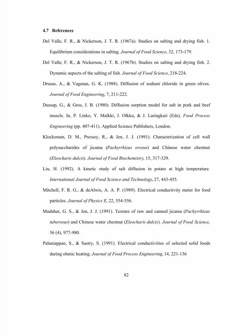
5/9/2018 Sarang Sanjay S - slidepdf.com
http://slidepdf.com/reader/full/sarang-sanjay-s 100/170
82
4.7 References
Del Valle, F. R., & Nickerson, J. T. R. (1967a). Studies on salting and drying fish. 1.
Equilibrium considerations in salting. Journal of Food Science, 32, 173-179.
Del Valle, F. R., & Nickerson, J. T. R. (1967b). Studies on salting and drying fish. 2.
Dynamic aspects of the salting of fish. Journal of Food Science, 218-224.
Drusas, A., & Vagenas, G. K. (1988). Diffusion of sodium chloride in green olives.
Journal of Food Engineering , 7, 211-222.
Dussap, G., & Gros, J. B. (1980). Diffusion sorption model for salt in pork and beef
muscle. In, P. Linko, Y. Malkki, J. Olkku, & J. Laringkari (Eds), Food Process
Engineering (pp. 407-411). Applied Science Publishers, London.
Klockeman, D. M., Pressey, R., & Jen, J. J. (1991). Characterization of cell wall
polysaccharides of jicama ( Pachyrrhizus erosus) and Chinese water chestnut
( Eleocharis dulcis). Journal of Food Biochemistry, 15, 317-329.
Liu, H. (1992). A kinetic study of salt diffusion in potato at high temperature.
International Journal of Food Science and Technology, 27, 443-455.
Mitchell, F. R. G., & deAlwis, A. A. P. (1989). Electrical conductivity meter for food
particles. Journal of Physics E , 22, 554-556.
Mudahar, G. S., & Jen, J. J. (1991). Texture of raw and canned jicama ( Pachyrrhizus
tuberosus) and Chinese water chestnut ( Eleocharis dulcis). Journal of Food Science,
56 (4), 977-980.
Palaniappan, S., & Sastry, S. (1991). Electrical conductivities of selected solid foods
during ohmic heating. Journal of Food Process Engineering , 14, 221-136
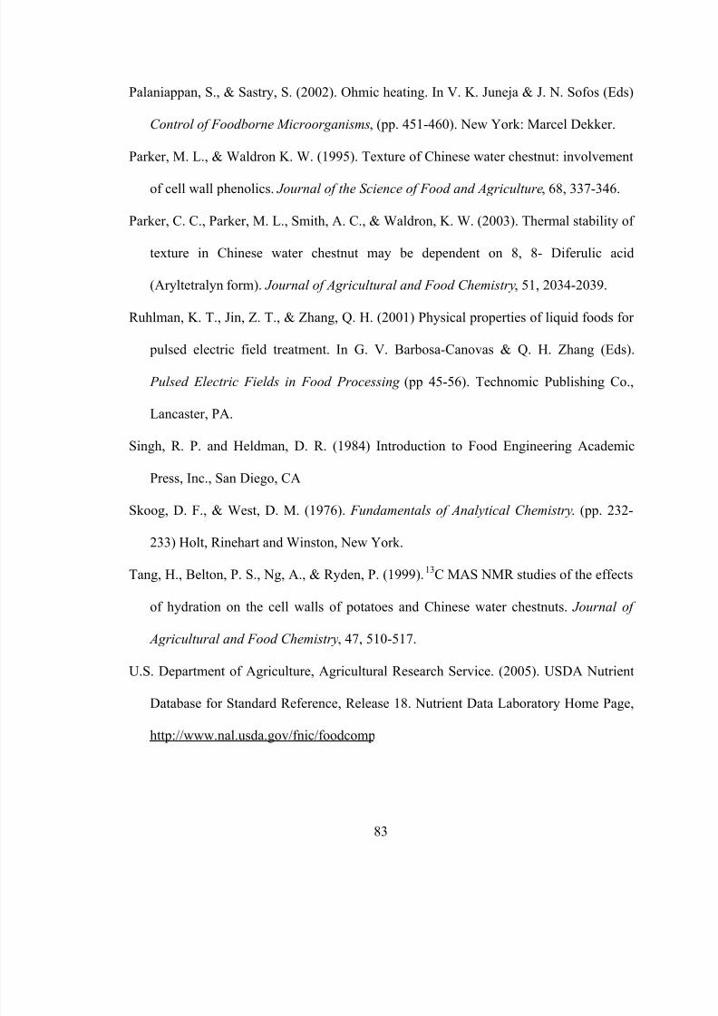
5/9/2018 Sarang Sanjay S - slidepdf.com
http://slidepdf.com/reader/full/sarang-sanjay-s 101/170
83
Palaniappan, S., & Sastry, S. (2002). Ohmic heating. In V. K. Juneja & J. N. Sofos (Eds)
Control of Foodborne Microorganisms, (pp. 451-460). New York: Marcel Dekker.
Parker, M. L., & Waldron K. W. (1995). Texture of Chinese water chestnut: involvement
of cell wall phenolics. Journal of the Science of Food and Agriculture, 68, 337-346.
Parker, C. C., Parker, M. L., Smith, A. C., & Waldron, K. W. (2003). Thermal stability of
texture in Chinese water chestnut may be dependent on 8, 8- Diferulic acid
(Aryltetralyn form). Journal of Agricultural and Food Chemistry, 51, 2034-2039.
Ruhlman, K. T., Jin, Z. T., & Zhang, Q. H. (2001) Physical properties of liquid foods for
pulsed electric field treatment. In G. V. Barbosa-Canovas & Q. H. Zhang (Eds).
Pulsed Electric Fields in Food Processing (pp 45-56). Technomic Publishing Co.,
Lancaster, PA.
Singh, R. P. and Heldman, D. R. (1984) Introduction to Food Engineering Academic
Press, Inc., San Diego, CA
Skoog, D. F., & West, D. M. (1976). Fundamentals of Analytical Chemistry. (pp. 232-
233) Holt, Rinehart and Winston, New York.
Tang, H., Belton, P. S., Ng, A., & Ryden, P. (1999).13
C MAS NMR studies of the effects
of hydration on the cell walls of potatoes and Chinese water chestnuts. Journal of
Agricultural and Food Chemistry, 47, 510-517.
U.S. Department of Agriculture, Agricultural Research Service. (2005). USDA Nutrient
Database for Standard Reference, Release 18. Nutrient Data Laboratory Home Page,
http://www.nal.usda.gov/fnic/foodcomp
5/9/2018 Sarang Sanjay S - slidepdf.com
http://slidepdf.com/reader/full/sarang-sanjay-s 102/170
84
Wang, W., & Sastry, S. (1993, a). Salt diffusion into vegetable tissue as a pretreatment
for ohmic heating: electrical conductivity profiles and vacuum infusion studies.
Journal of Food Engineering , 20, 299-309.
Wang, W., & Sastry, S. (1993, b). Salt diffusion into vegetable tissue as a pretreatment
for ohmic heating: determination of parameters and mathematical model verification.
Journal of Food Engineering , 20, 311-323.
Williams, W. J. (1979). Handbook of Anion Determination. (pp. 297-301) Butterworths,
London.
Wistreich, H. E., Morse, R. E., & Kenyon, L. J. (1960) Curing of ham: a study of sodium
chloride accumulation. II: Combined effects of time, solution concentration and
solution volume. Food Technology, 14, 549-551.
Wood, F. W. (1966). The diffusion of salt in pork muscle and fat tissue. Journal of the
Science of Food and Agriculture, 17, 138-140.
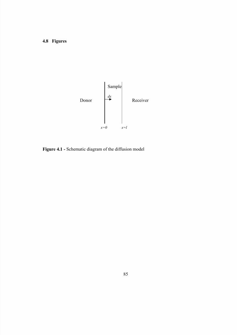
5/9/2018 Sarang Sanjay S - slidepdf.com
http://slidepdf.com/reader/full/sarang-sanjay-s 103/170
4.8 Figures
Donor Receiver
Sample
dx
x=0 x=l
Figure 4.1 - Schematic diagram of the diffusion model
85
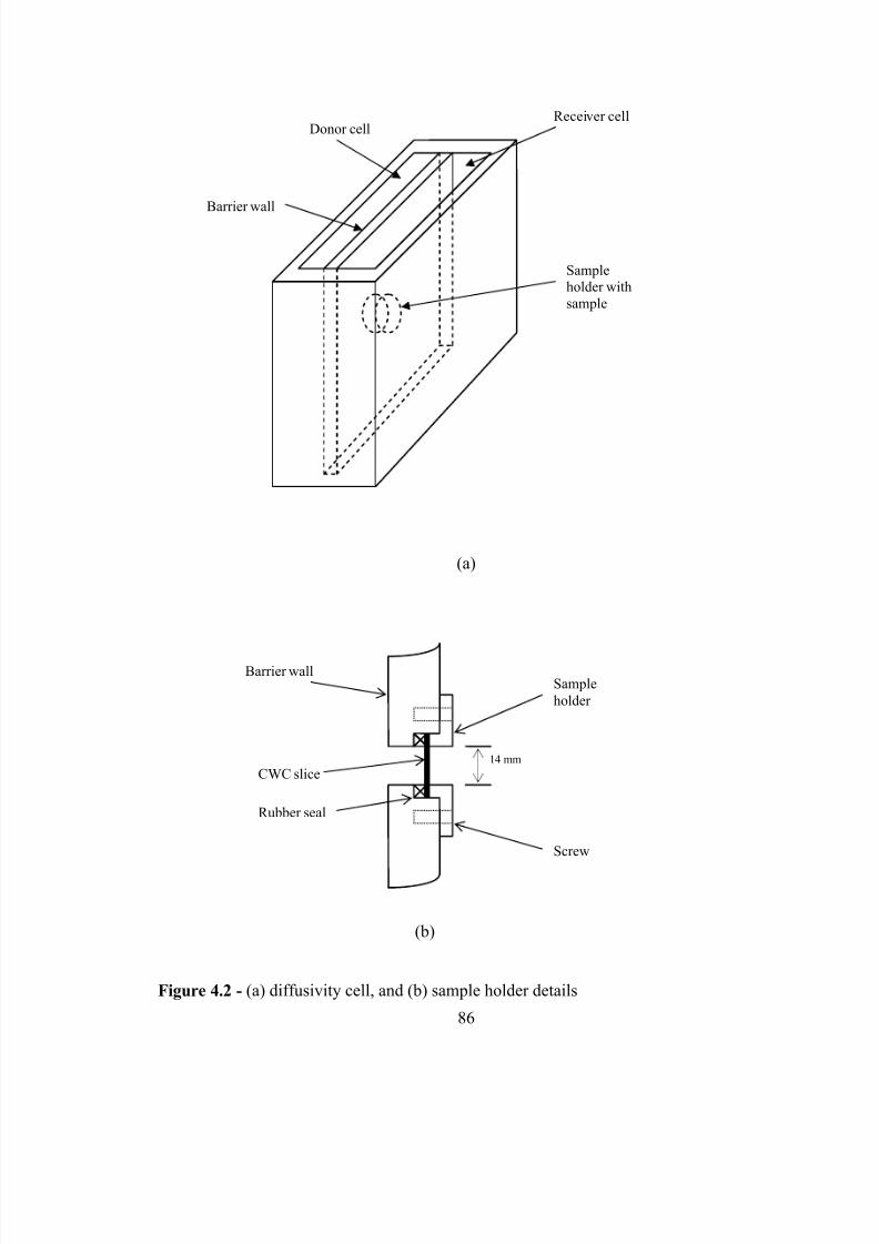
5/9/2018 Sarang Sanjay S - slidepdf.com
http://slidepdf.com/reader/full/sarang-sanjay-s 104/170
Sample
holder with
sample
Barrier wall
Donor cellReceiver cell
(a)
14 mm
Screw
Sample
holder
Rubber seal
CWC slice
Barrier wall
(b)
Figure 4.2 - (a) diffusivity cell, and (b) sample holder details
86
5/9/2018 Sarang Sanjay S - slidepdf.com
http://slidepdf.com/reader/full/sarang-sanjay-s 105/170
Electrode 1Electrode 2
Wall
Wall
0.18m
0.18m
Disc
(0.018m x 0.0075m
Figure 4.3 – Schematic diagram of chestnut disc in box used for simulation studies.
87
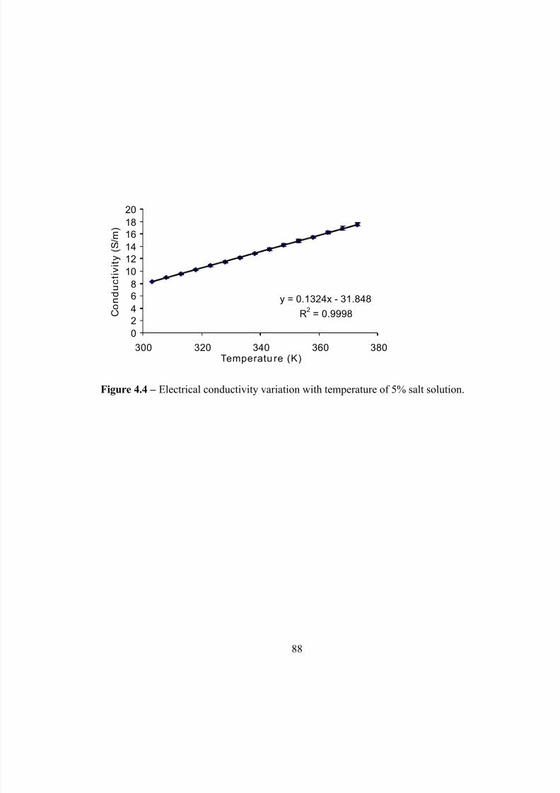
5/9/2018 Sarang Sanjay S - slidepdf.com
http://slidepdf.com/reader/full/sarang-sanjay-s 106/170
y = 0.1324x - 31.848
R2
= 0.9998
0
2
4
6
810
12
14
1618
20
300 320 340 360 380Temperature (K)
C o n d u c t i v i t y ( S / m )
Figure 4.4 – Electrical conductivity variation with temperature of 5% salt solution.
88
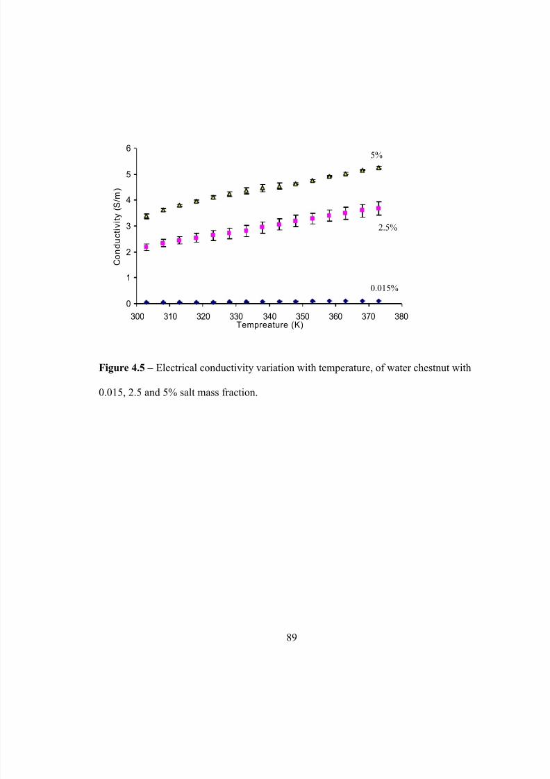
5/9/2018 Sarang Sanjay S - slidepdf.com
http://slidepdf.com/reader/full/sarang-sanjay-s 107/170
0
1
2
3
4
5
6
300 310 320 330 340 350 360 370 380Tempreature (K)
C o n d u c t i v i t y ( S / m )
5%
2.5%
0.015%
Figure 4.5 – Electrical conductivity variation with temperature, of water chestnut with
0.015, 2.5 and 5% salt mass fraction.
89
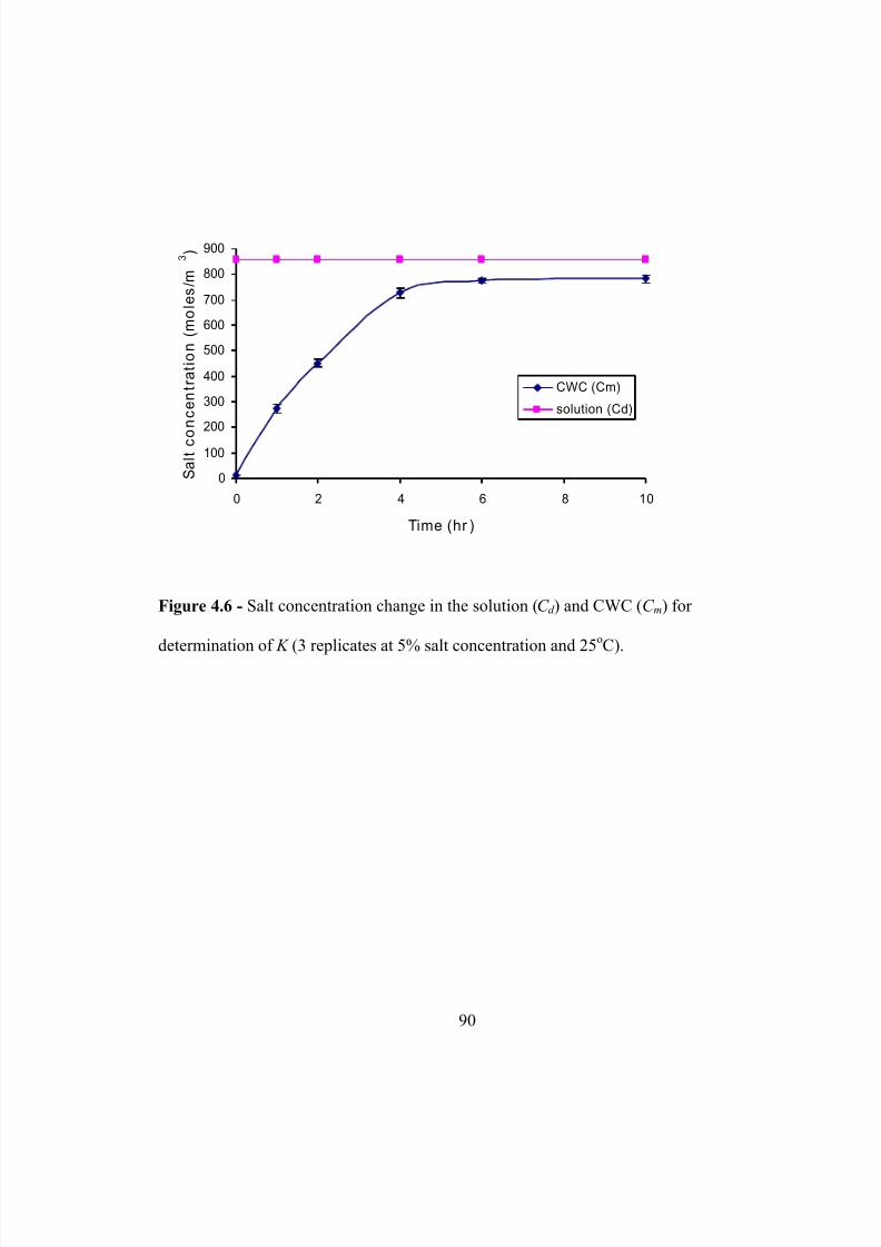
5/9/2018 Sarang Sanjay S - slidepdf.com
http://slidepdf.com/reader/full/sarang-sanjay-s 108/170
0
100
200
300
400
500
600
700
800
900
0 2 4 6 8 10
Time (hr)
S a l t c o
n c e n t r a t i o n ( m o l e s / m
3 )
CWC (Cm)
solution (Cd)
Figure 4.6 - Salt concentration change in the solution (C d ) and CWC (C m) for
determination of K (3 replicates at 5% salt concentration and 25
o
C).
90
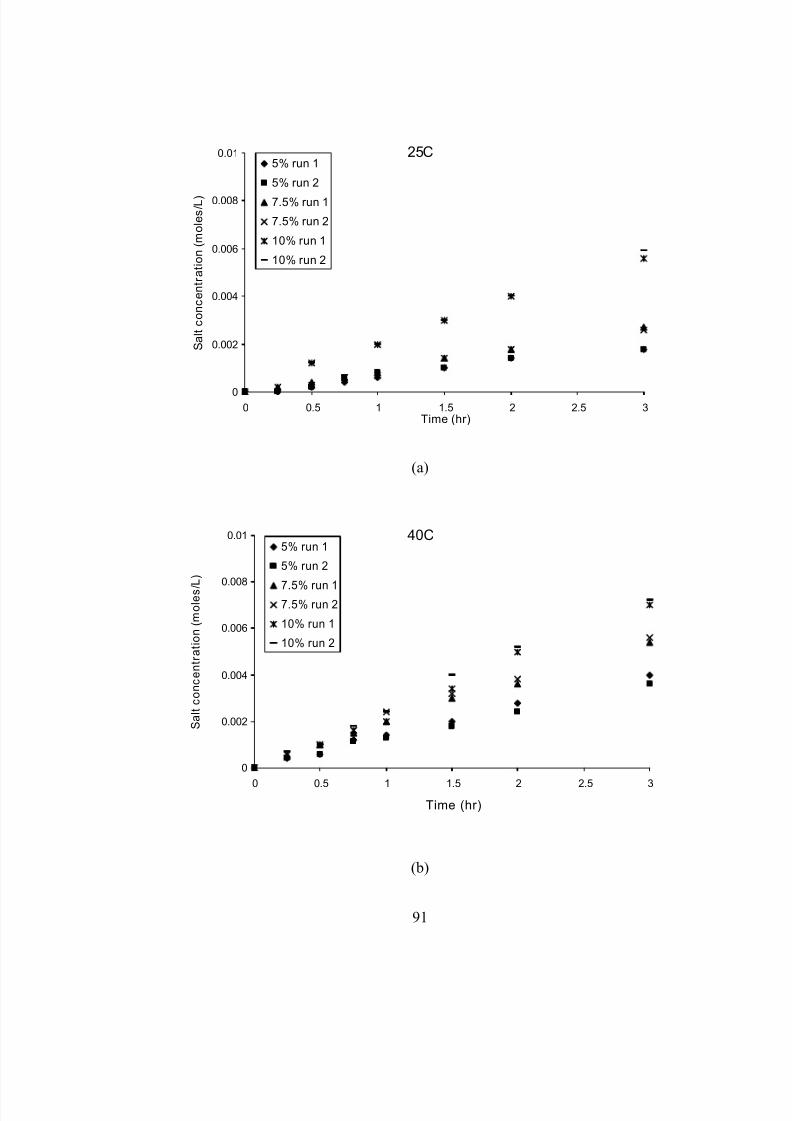
5/9/2018 Sarang Sanjay S - slidepdf.com
http://slidepdf.com/reader/full/sarang-sanjay-s 109/170
25C
0
0.002
0.004
0.006
0.008
0.01
0 0.5 1 1.5 2 2.5 3Time (hr)
S a l t c o n c e n t r a t i o n ( m o l e s / L )
5% run 1
5% run 2
7.5% run 1
7.5% run 2
10% run 1
10% run 2
(a)
40C
0
0.002
0.004
0.006
0.008
0.01
0 0.5 1 1.5 2 2.5
Time (hr)
S a l t c o n c e n t r a t i o n ( m o l e s / L )
3
5% run 1
5% run 2
7.5% run 17.5% run 2
10% run 1
10% run 2
(b)
91
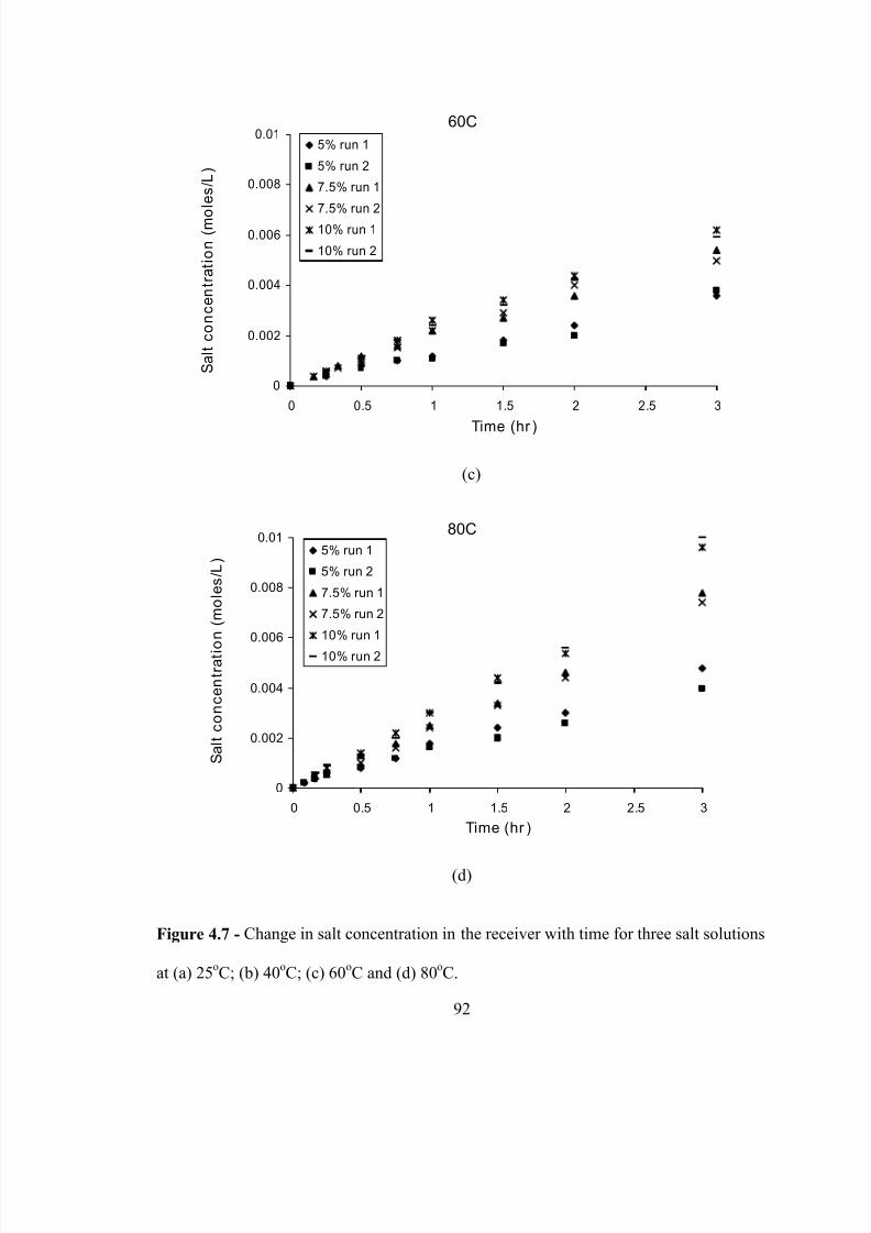
5/9/2018 Sarang Sanjay S - slidepdf.com
http://slidepdf.com/reader/full/sarang-sanjay-s 110/170
60C
0
0.002
0.004
0.006
0.008
0.01
0 0.5 1 1.5 2 2.5
Time (hr)
S a l t c o n c e n t r a t i o n ( m o
l e s / L )
3
5% run 1
5% run 2
7.5% run 1
7.5% run 210% run 1
10% run 2
(c)
80C
0
0.002
0.004
0.006
0.008
0.01
0 0.5 1 1.5 2 2.5 3
Time (hr)
S a l t c o n c e n t r a t i o
n ( m o l e s / L )
5% run 1
5% run 2
7.5% run 1
7.5% run 2
10% run 1
10% run 2
(d)
Figure 4.7 - Change in salt concentration in the receiver with time for three salt solutions
at (a) 25oC; (b) 40
oC; (c) 60
oC and (d) 80
oC.
92
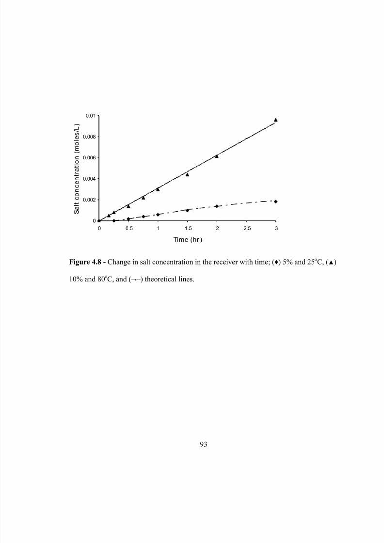
5/9/2018 Sarang Sanjay S - slidepdf.com
http://slidepdf.com/reader/full/sarang-sanjay-s 111/170
0
0.002
0.004
0.006
0.008
0.01
0 0.5 1 1.5 2 2.5 3
Time (hr)
S a l t c o n
c e n t r a t i o n ( m o l e s / L )
Figure 4.8 - Change in salt concentration in the receiver with time; (♦) 5% and 25oC, (▲)
10% and 80oC, and (– ▪ –) theoretical lines.
93
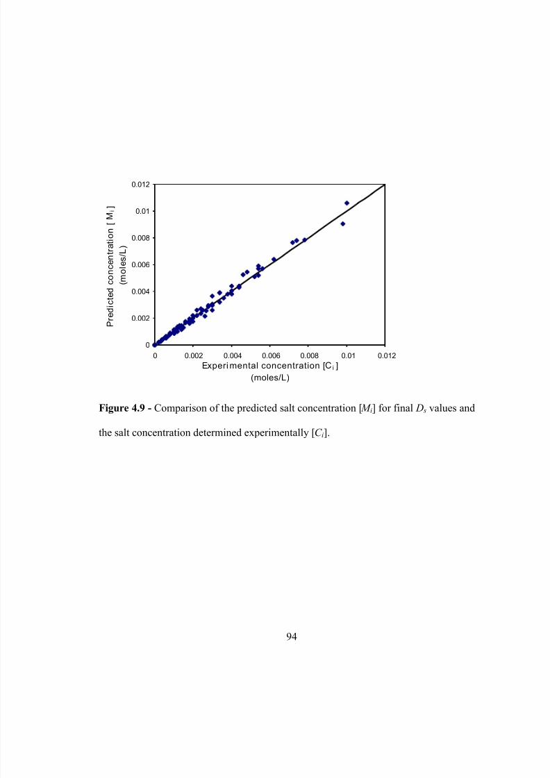
5/9/2018 Sarang Sanjay S - slidepdf.com
http://slidepdf.com/reader/full/sarang-sanjay-s 112/170
0
0.002
0.004
0.006
0.008
0.01
0.012
0 0.002 0.004 0.006 0.008 0.01 0.012
Experimental concentration [C i ]
(moles/L)
P r e d i c t e d c o n
c e n t r a t i o n [ M i ]
( m o
l e s / L )
Figure 4.9 - Comparison of the predicted salt concentration [M i] for final D s values and
the salt concentration determined experimentally [C i].
94
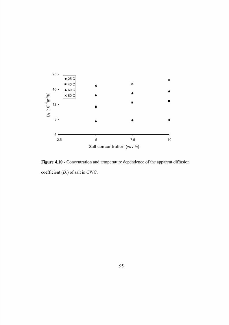
5/9/2018 Sarang Sanjay S - slidepdf.com
http://slidepdf.com/reader/full/sarang-sanjay-s 113/170
4
8
12
16
20
2.5 5 7.5 10
Salt concentration (w/v %)
D s ( 1 0 - 1 0 m 2 / s )
25 C
40 C
60 C
80 C
Figure 4.10 - Concentration and temperature dependence of the apparent diffusion
coefficient ( D s) of salt in CWC.
95
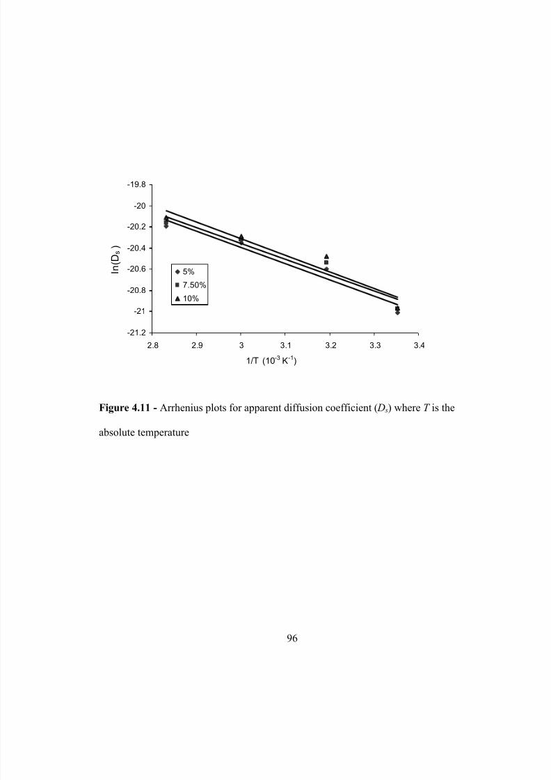
5/9/2018 Sarang Sanjay S - slidepdf.com
http://slidepdf.com/reader/full/sarang-sanjay-s 114/170
-21.2
-21
-20.8
-20.6
-20.4
-20.2
-20
-19.8
2.8 2.9 3 3.1 3.2 3.3 3.4
1/T (10-3 K-1)
l n ( D s )
5%7.50%
10%
Figure 4.11 - Arrhenius plots for apparent diffusion coefficient ( D s) where T is the
absolute temperature
96
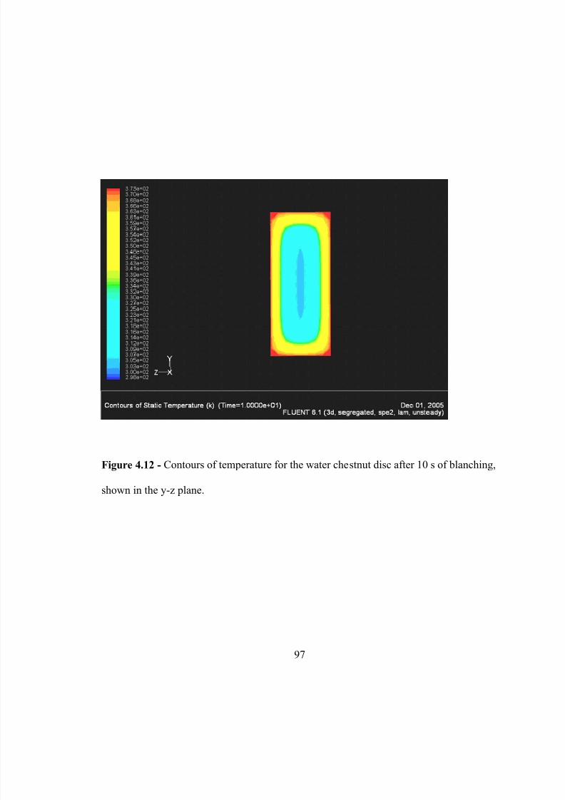
5/9/2018 Sarang Sanjay S - slidepdf.com
http://slidepdf.com/reader/full/sarang-sanjay-s 115/170
Figure 4.12 - Contours of temperature for the water chestnut disc after 10 s of blanching,
shown in the y-z plane.
97
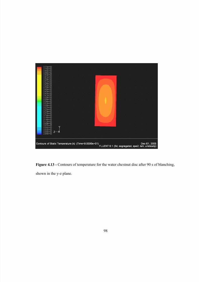
5/9/2018 Sarang Sanjay S - slidepdf.com
http://slidepdf.com/reader/full/sarang-sanjay-s 116/170
Figure 4.13 - Contours of temperature for the water chestnut disc after 90 s of blanching,
shown in the y-z plane.
98
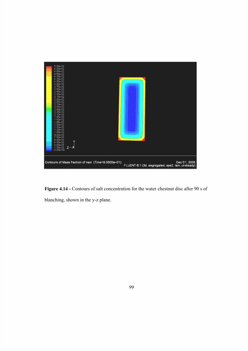
5/9/2018 Sarang Sanjay S - slidepdf.com
http://slidepdf.com/reader/full/sarang-sanjay-s 117/170
Figure 4.14 - Contours of salt concentration for the water chestnut disc after 90 s of
blanching, shown in the y-z plane.
99
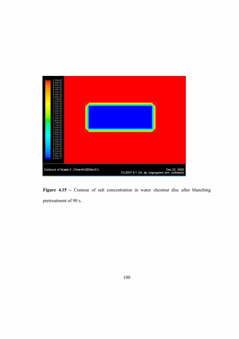
5/9/2018 Sarang Sanjay S - slidepdf.com
http://slidepdf.com/reader/full/sarang-sanjay-s 118/170
Figure 4.15 – Contour of salt concentration in water chestnut disc after blanching
pretreatment of 90 s.
100
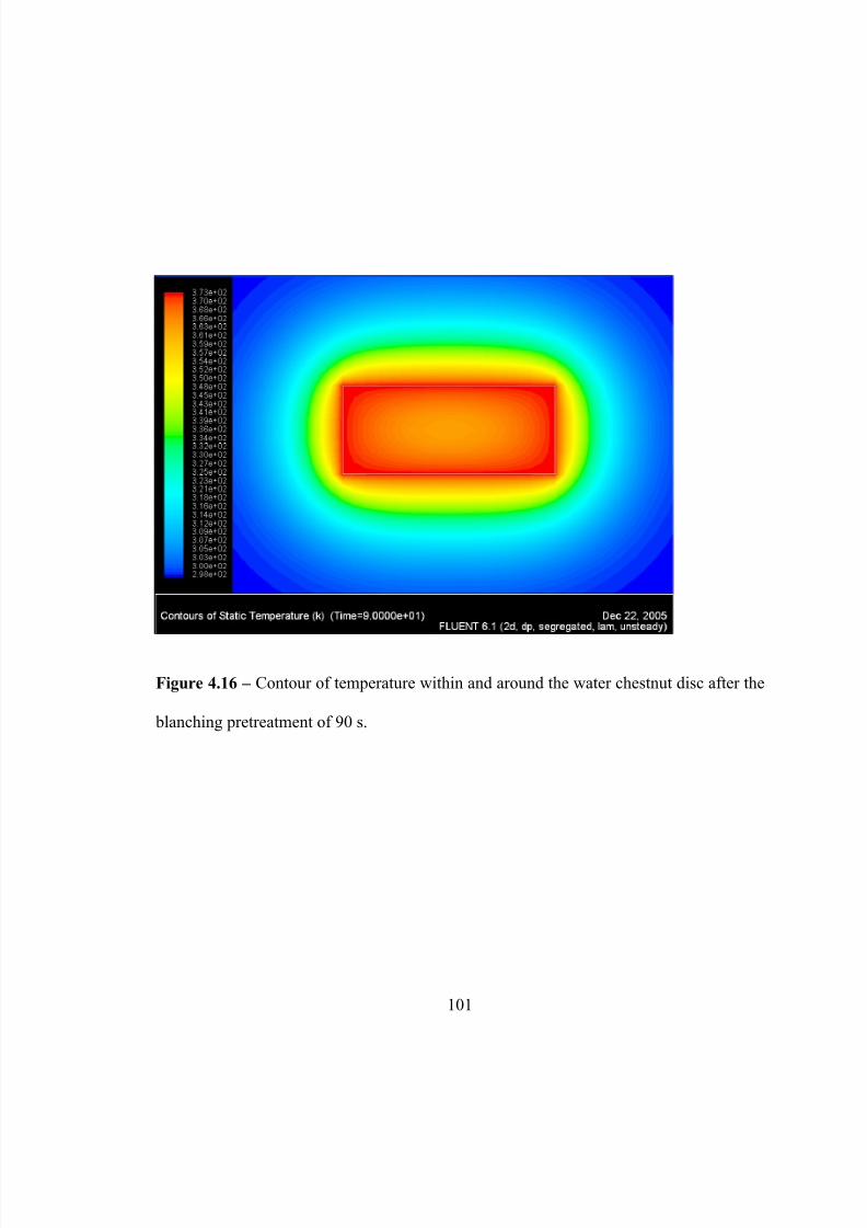
5/9/2018 Sarang Sanjay S - slidepdf.com
http://slidepdf.com/reader/full/sarang-sanjay-s 119/170
Figure 4.16 – Contour of temperature within and around the water chestnut disc after the
blanching pretreatment of 90 s.
101

5/9/2018 Sarang Sanjay S - slidepdf.com
http://slidepdf.com/reader/full/sarang-sanjay-s 120/170
Figure 4.17 – Contour of electrical conductivity inside the chestnut disc.
102
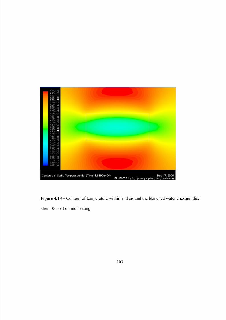
5/9/2018 Sarang Sanjay S - slidepdf.com
http://slidepdf.com/reader/full/sarang-sanjay-s 121/170
Figure 4.18 – Contour of temperature within and around the blanched water chestnut disc
after 100 s of ohmic heating.
103
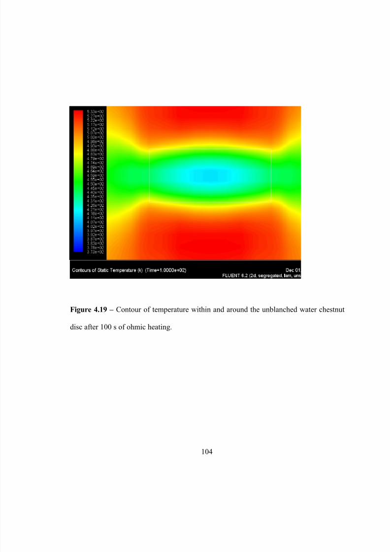
5/9/2018 Sarang Sanjay S - slidepdf.com
http://slidepdf.com/reader/full/sarang-sanjay-s 122/170
Figure 4.19 – Contour of temperature within and around the unblanched water chestnut
disc after 100 s of ohmic heating.
104
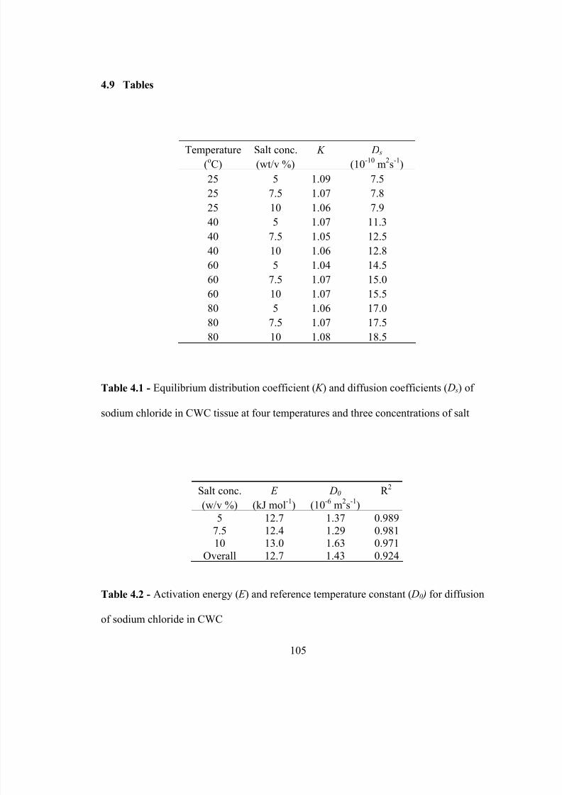
5/9/2018 Sarang Sanjay S - slidepdf.com
http://slidepdf.com/reader/full/sarang-sanjay-s 123/170
105
4.9 Tables
Temperature Salt conc. K D s
(oC) (wt/v %) (10
-10m
2s
-1)
25 5 1.09 7.5
25 7.5 1.07 7.8
25 10 1.06 7.9
40 5 1.07 11.3
40 7.5 1.05 12.5
40 10 1.06 12.8
60 5 1.04 14.5
60 7.5 1.07 15.060 10 1.07 15.5
80 5 1.06 17.0
80 7.5 1.07 17.5
80 10 1.08 18.5
Table 4.1 - Equilibrium distribution coefficient ( K ) and diffusion coefficients ( D s) of
sodium chloride in CWC tissue at four temperatures and three concentrations of salt
Salt conc. E D0 R 2
(w/v %) (kJ mol-1
) (10-6
m2s
-1)
5 12.7 1.37 0.989
7.5 12.4 1.29 0.98110 13.0 1.63 0.971
Overall 12.7 1.43 0.924
Table 4.2 - Activation energy ( E ) and reference temperature constant ( D0 ) for diffusion
of sodium chloride in CWC
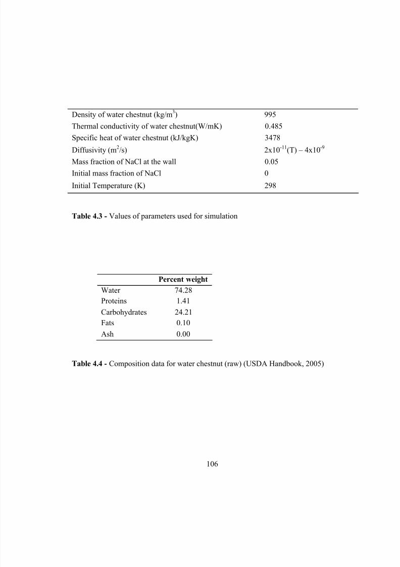
5/9/2018 Sarang Sanjay S - slidepdf.com
http://slidepdf.com/reader/full/sarang-sanjay-s 124/170
106
Density of water chestnut (kg/m3) 995
Thermal conductivity of water chestnut(W/mK) 0.485
Specific heat of water chestnut (kJ/kgK) 3478
Diffusivity (m2/s) 2x10
-11(T) – 4x10
-9
Mass fraction of NaCl at the wall 0.05
Initial mass fraction of NaCl 0
Initial Temperature (K) 298
Table 4.3 - Values of parameters used for simulation
Percent weight
Water 74.28
Proteins 1.41
Carbohydrates 24.21
Fats 0.10
Ash 0.00
Table 4.4 - Composition data for water chestnut (raw) (USDA Handbook, 2005)
5/9/2018 Sarang Sanjay S - slidepdf.com
http://slidepdf.com/reader/full/sarang-sanjay-s 125/170
107
CHAPTER 5
RESIDENCE TIME DISTRIBUTION (RTD) OF PARTICULATE FOODS IN A
CONTINUOUS FLOW PILOT-SCALE OHMIC HEATER
5.1 Abstract
The Residence Time Distribution (RTD) of a model particulate-fluid mixture
(potato in starch solution) in the ohmic heater in a continuous sterilization process was
measured using a Radio Frequency Identification (RFID) methodology. The effect of
solid concentration and the rotational speed of the agitators on the RTD were studied.
The velocity of the fastest particle was 1.62 times the mean product velocity. In general,
particle velocity was found to be greater than the product bulk average velocity. Mean
particle residence time increased with increase in the rotational speed of the agitators (p <
0.05) and no particular trend was observed between the mean particle residence time and
the solid concentration. The distribution curves E (θ) were skewed to the right suggesting
slow moving zones in the system.
5/9/2018 Sarang Sanjay S - slidepdf.com
http://slidepdf.com/reader/full/sarang-sanjay-s 126/170
108
5.2 Introduction
In continuous sterilization processes critical parameters include the temperature of
the coldest spot in the food and the shortest particle residence time in heating and holding
sections. Measurement of residence time distribution (RTD) is needed for determination
of the fastest-moving particle, to be used for designing and biologically validating
processes. Residence times of the average and slowest food elements helps in evaluating
quality degradation.
The critical safety consideration is that of the fastest-moving particle: the RTD
experiment must be able to demonstrate with a high degree of confidence (95 %) that the
fastest (99th
percentile) particle has indeed been sampled and therefore the sample size
becomes critical. DiGeronimo et al. (1997) stated that a distribution-free method was the
most appropriate method to determine reliably the characteristic fastest particle of the
system. Palaniappan & Sizer (1997) determined with 95% confidence that the fastest 99th
percentile particle was sampled, a population size of 299 particles is necessary.
Most studies on RTD have focused on visualization or detecting flow of particles
either within or at the inlet and outlet of process equipment. Alhamdan & Sastry (1997),
Salengke & Sastry (1995), Salengke & Sastry (1996), Dutta & Sastry (1990a,b), McCoy
et al. (1987), and Sancho & Rao (1991) studied RTD of food particles in holding tube. A
number of published studies have addressed residence times in swept surface heat
exchanges (SSHE) (Alhamdan & Sastry, 1998; Lee & Singh, 1991; Chandarana &
Unverferth, 1996).
Only a few experiments have been performed on RTD in ohmic heating systems.
RTD of particulates in ohmic system was investigated by Kim et al. (1996) both visually

5/9/2018 Sarang Sanjay S - slidepdf.com
http://slidepdf.com/reader/full/sarang-sanjay-s 127/170
109
and using Hall effect sensors for 35% total solids content in a sauce. Marcotte et al.
(2000) used an ultrasonic method to determine RTD of particulate foods (carrot particles/
starch solution mixtures) during ohmic heating. Tulsiyan et al. (2007) measured RTD of
chicken particles in chicken chowmein product in the ohmic heaters, using Radio
Frequency Identification (RFID) technology. More detailed studies of RTD of food
particles within an ohmic heater are necessary.
Three categories of variables which can affect RTD of particles in particulate
system are identifiable, those associated with the physical system, particles, and the
carrier fluid. System variables include dimensions, orientation, rotational speed of
agitators and product flow rate; particle variables include concentration, size, shape, type
and density; and the principal fluid variable involves rheological properties. System
variables like dimensions and orientation of heaters are generally fixed for the ohmic
heating facility. There is a need to study, in detail, the effect of other variables.
Several techniques have been developed for investigating the RTD of solid-liquid
flow as reviewed by Ramaswamy et al. (1995) and Sastry & Cornelius (2002). These
include visual observation (for example, stop watch, photography, playback videotaping),
laser beam detection, radioactive tracers, magnetic response, and photo sensors
methodology. Most methods work at low temperatures although recent investigations
have been performed at high temperatures. Generally, the majority of published results
were for a low proportion of solids with respect to liquid. A popular technique with the
industry is the use of magnetic methods which involve introduction of tagged particles
containing small magnets (Segner et al., 1989; Chandarana & Unverferth, 1996). The
passage of these tagged particles is detected by a voltage generated within coils at
5/9/2018 Sarang Sanjay S - slidepdf.com
http://slidepdf.com/reader/full/sarang-sanjay-s 128/170
110
selected locations of the process equipment. Hall effect sensors also operate on a similar
principle of electro magnetic induction (Tucker & Withers, 1994). Magnetic resonance
techniques have also been used for flow visualization in food systems (Manavel et al.,
1993). Optical methods like particle tracking velocimetry (Zitoun et al., 2001) and other
visualization techniques have also been used. Researchers have also examined history
methods, such as chemical markers and thermal memory cells, which involve
determining the effect of a process on a chemical reaction or diffusion process and back
calculating processing parameters (Kim & Taub, 1993; Swartzel et al., 1991). Other
methods for measuring RTD are ultrasound methods, which involve detecting RTD by
Doppler scattering of ultrasound waves by the moving particles, and salt tracer methods,
where the RTD is measured by electrical conductivity measurements (Ramaswamy et al,
1995).
In industry, magnetic particle methods have achieved greater acceptance than the
other methods because of their simplicity, versatility, relative ease of implementation and
low cost. However, their principal limitation is the inability to distinguish between
multiple particles passing through the detector at the same time. This necessitates that
operator wait for each magnetic tracer to enter and exit the system before introduction of
the next tracer (Sastry & Cornelius, 2002).
Radio Frequency Identification (RFID) technology contains tags, each with a
unique serial number or an Electronic Product Code (EPC), which can be read by the
reader (Bhuptani & Moradpour, 2005; Heinrich, 2005; and Paret, 2005). Since each tag
has a unique code, multiple particles with embedded RFID tags can be introduced in the
food processing system at the same time for RTD measurement. One reader can be
5/9/2018 Sarang Sanjay S - slidepdf.com
http://slidepdf.com/reader/full/sarang-sanjay-s 129/170
111
placed at the inlet and another at the outlet of the system across which the RTD is to be
measured. When the particle containing the RFID tag passes through the reader, the EPC
code is transmitted to the reader, and the time of transmission is recorded. The difference
between the time recorded at the inlet and the outlet reader provides residence time for
that particle. RFID technique, where in it is possible to track multiple particles, could be
used to measure RTD of particles in the ohmic heater in a continuous sterilization
process. Grabowski et al. (1993) patented similar approach for measuring RTD. The
limitation of their studies was that the transponders they used were of the order of 0.0254
m long and 0.00356 m diameter making them longer than the normally desirable
processed food particles. Today the availability of small and lighter transponders, make
RFID technique attractive for measuring RTD of food particles. Tulsiyan et al. (2007)
used RFID methodology to determine RTD of chicken particles in ohmic heating system.
The use of RFID tracers obviated the waiting time that was needed for a magnetic tracer
to exit the system before the next magnetic tracer can be introduced.
The objective of this study was to study the effect of concentration of solids (30,
40, 50, 60, 70, and 80 % v/v) and rotational speed of the agitators (55, 40, and 25 rpm) on
the RTD of particles in a solid-liquid food mixture (potato in starch solution) in a pilot-
scale ohmic heater.
5/9/2018 Sarang Sanjay S - slidepdf.com
http://slidepdf.com/reader/full/sarang-sanjay-s 130/170
112
5.3 Materials and methods
5.3.1 Product
The product chosen for this study was potato solids in starch solution. Diced
frozen potatoes (5/8 inch) were procured from E.W. Carlberg Co. (Kansas City). The
carrier fluid was a starch solution with 6 %w/w starch (PURITY CLOUD®
, National
Starch, Bridgewater, NJ) and 0.45 %w/w NaCl salt (Cargill, Minneapolis, MN). Frozen
potatoes were blanched for 30 s in 3 %w/w NaCl salt solution at about 98oC, to raise the
temperature and to increase the electrical conductivity and match it to the carrier fluid.
The formulation was finalized based on preliminary experimental results, to obtain a
viscous carrier fluid and closely match the conductivities of solid and fluid phases.
5.3.2 Analog particles
Potato/alginate analog particles carrying RFID tags were used as tracers for the
RTD studies. The potato/alginate cubes were prepared by adaptation of the formula used
by Brown et al. (1984). Canned sliced potatoes (The Kroger Co., Cincinnati, OH) were
drained and mashed in a blender and mixed to obtain potato/alginate blend. The finished
potato/alginate blend was shaped into a 5/8” slab. RFID tags were inserted into the slab at
equal distances (5/8”) and the slab was immersed in a 2 % calcium chloride solution
overnight at 4oC to harden. After hardening, the slab was then cut into 5/8” cubes (such
that each RFID tag was at the center of the cube). The analog particles thus obtained were
stored in calcium chloride solution at refrigerated temperature until use. A colored food-
dye (The Kroger Co., Cincinnati, OH) was added to the mixture to help identify the
tracers for recovery of the RFID tags after the experiment.
5/9/2018 Sarang Sanjay S - slidepdf.com
http://slidepdf.com/reader/full/sarang-sanjay-s 131/170
113
Electrical conductivity of the particles so obtained was found to be significantly
higher than the blanched potato particles and the gelatinized starch solution. In order to
adjust the conductivity, while still maintaining the density and rigidity of the particles,
different formulations were prepared containing vegetable oil, polystyrene beads (125 –
212 μm) or sand (15 – 150 μm), in different proportions. The formulation was finalized
based on these preliminary experiments to obtain analog particles of the same density and
electrical conductivity as the blanched potato solids and the carrier fluid. The formulation
is shown in Table 5.1.
Density was determined by weight/volume method and the density of
potato/alginate particles was within 2.7% of the blanched potato solids. An electrical
conductivity comparison of the starch solution, blanched potatoes, and potato/alginate
analog particles is shown in Figure 5.1. Electrical conductivity of 10 samples each was
determined using the experimental setup and procedures explained in Chapter 2.
Statistical analysis showed that there was no significant difference in the electrical
conductivities of the three components (p > 0.05).
5.3.3 Ohmic heating pilot plant facility
Experiments were performed on a 54 kW industrial ohmic heating pilot plant with
small modifications to the system to accommodate the RFID readers. The installation
consisted of two mixing tanks, a magnetic flow meter (Rosemount Inc, Chanhassen, MN,
USA), heating column, swept surface heat exchanger (SSHE) (Waukesha Cherry-Burrell,
Delavan, WI, USA), holding tube, and aseptic catch tank (see Figure 5.2). The heating
column consisted of three ohmic heaters with each heating section housed between a pair
of electrodes.

5/9/2018 Sarang Sanjay S - slidepdf.com
http://slidepdf.com/reader/full/sarang-sanjay-s 132/170
114
5.3.4 Radio Frequency Identification (RFID)
Cylindrical shaped RFID tags (GLT12x2RO, Intersoft Corp, Tullahoma, TN,
USA), measuring 0.012m in length and 0.002m in diameter, and weighing 0.0001 kg
were used. The tags operated at 125 kHz frequency which is considered least susceptible
to metal and liquid interference. The RFID reader consisted of a reader module
(TRRO1OEM, Intersoft Corp, Tullahoma, TN, USA) and a circular antenna (Intersoft
Corp, Tullahoma, TN, USA) connected to the module board.
In the pilot plant facility, the metal tubes present at the inlet and outlet of the
ohmic heating column were replaced by glass tubes. This is necessary to minimize the
attenuation that radio frequency suffers near metal. One antenna was placed at the inlet of
the heater and a second antenna at the outlet (Fig. 5.2). A RFID reader was connected to
each antenna. Both readers were connected to a computer for data acquisition. The
software used for data acquisition was a modified version of the software provided by the
RFID vendor (tstdemo2.exe, Intersoft Corp, Tullahoma, TN, USA) which would record
the EPC serial code of the tags and the time the code is read.
5.3.5 Experimental method
All the variables and parameters of this study are listed in Table 5.2. In a separate
set of preliminary experiments the bulk conductivity of the product (with different solid
concentrations) was determined using a bench scale 2 inch static ohmic heater (the setup
described in Chapter 3). Electrical conductivity of different concentrations of sodium
sulfate solution in water (sterilizing fluid) was also determined. Different sodium sulfate
solution concentrations that match the electrical conductivity of the different products are
listed in Table 5.3.
5/9/2018 Sarang Sanjay S - slidepdf.com
http://slidepdf.com/reader/full/sarang-sanjay-s 133/170
115
Sodium sulfate solution of the required concentration was prepared in a mixing
tank, pumped through the system and ohmically heated. System conditions, such as flow
rate (1.9gal/min), inlet temperature to the heaters (55oC), outlet temperature from the
heaters (130oC) and outlet temperature from heat exchangers (approximately 30
oC) were
set using this salt solution.
Starch solution was first cooked and gelatinized at about 70oC in a separate
mixing tank. Frozen potatoes were blanched separately for 30 s in 3 %w/w salt solution at
boiling temperature. Blanched potatoes along with potato/alginate analog particles were
then added to the gelatinized starch solution and mixed in the mixing tank. Although data
were only needed for 299 intact particles, 600-650 tracers were added in the mixing tank
and mixed thoroughly with the product. The extra tracers were added to provide a margin
of safety, since not all particles that remained fully intact would be read by the readers at
both the inlet and the outlet of the ohmic heaters. Once the product temperature was 55oC
(similar to the inlet condition of sodium sulfate solution) product was pumped through
the system. Generally, a half hour of mixing was allowed between mixing the solids in
cooked starch solution and pumping the product. This time was considered enough to mix
the product properly. The product, along with the tracers, was heated to aseptic
processing temperature (130oC) in the ohmic heaters, held in the holding tube, cooled in
the SSHE and water cooled tube heat exchangers, and finally collected in the aseptic
tank.
When the RFID tag-containing tracers passed through the reader antenna, the
reader powered the tags which then transmitted their EPC serial code to the reader, which
was recorded by the data acquisition system. The time at which the EPC was transmitted
5/9/2018 Sarang Sanjay S - slidepdf.com
http://slidepdf.com/reader/full/sarang-sanjay-s 134/170
116
was also recorded. The difference between the time recorded at the inlet and the outlet
reader for a tracer gave the residence time for that tracer particle. Data was collected for
minimum 299 intact particles, under each experimental condition.
The product flow rate was fixed through the experiments at 1.2 m3/s (1.9 gal/min).
Knowing the volume between the two readers the mean product residence time was
calculated to be 94 s. Once the entire product was pumped through the heaters, the line
was switched back to sodium sulfate solution and heating was stopped. Product was
collected in the aseptic tank from which the particles containing RFID tags were
retrieved. The experiment was repeated for different solid concentrations and rotational
speed settings.
5.4 Results
Three levels of rotation speed of agitators on ohmic heaters (55, 40, and 25 rpm)
and six levels of solid concentrations (30, 40, 50, 60, 70 and 80 % v/v) were studied for
their effect on the RTD of particles in ohmic heaters. After the experiments were
completed for solid concentrations up to 60% solid concentration it was observed that
solid concentration did not affect RTD significantly (which will be discussed shortly).
Hence, 70 and 80 % v/v solid concentration studies were performed only at one rotational
speed of the agitators (40 rpm). With 80 % solids the resulting product was very thick
and viscous. It was difficult to pump this product while maintaining the flow rate, final
processing temperature, and the pressure in the system constant. The run was aborted and
residence time data could not be collected.
5/9/2018 Sarang Sanjay S - slidepdf.com
http://slidepdf.com/reader/full/sarang-sanjay-s 135/170
117
Tables 5.4, through 5.9 summarize the effect of the variables studied, on the
minimum particle residence time, minimum normalized particle residence time
(MNNPRT), mean particle residence time (MPRT), mean normalized particle residence
time (MNPRT), maximum particle residence time (MXPRT) and maximum normalized
particle residence time (MXNPRT) respectively. The normalized times were calculated
by dividing the particle residence times with the mean product residence time (94 s).
The fastest particle residence time was 58 s, or the velocity of the fastest particle
was 1.62 times the mean product velocity. The fastest particle was therefore substantially
below the limit of laminar flow of Newtonian fluids in cylindrical tube, where the
maximum velocity in the center of the tube can reach twice the mean velocity. In most of
the cases the mean normalized particle residence time (MNPRT) (see Table 5.7) was less
than the mean product residence time, which implies that average particle velocities are
faster than the bulk product velocity. In all runs, the MXPRT was found to be 188 s or the
MXNPRT was 2.00. This implies that the slowest moving particle is twice as slow as the
bulk product.
Mean particle residence time (MPRT) increased with increase in the rotational
speed of the agitators (p < 0.05), see Table 5.6. Also, the statistical analysis shows that
MPRT are affected significantly by the solid concentration (p < 0.05), however, no
particular trend was observed between the mean residence time and the solid
concentration.
The density function E (θ), for the normalized residence time are plotted for all
cases and shown in Figure 5.3 through 5.15. These plots illustrate the spread of the
residence time distributions from the mean and also help to examine its departure from
5/9/2018 Sarang Sanjay S - slidepdf.com
http://slidepdf.com/reader/full/sarang-sanjay-s 136/170
118
the ideal plug flow behavior. It can be observed that in all the cases the E (θ) curves are
skewed to the right and, in general, at higher solid concentrations the distribution
becomes narrower. Tusiyan et al. (2007) observed similar tailing effects when they
measured the RTD of chicken particles in chicken chowmein in the same ohmic heating
system. In their studies the MXNPRT was 1.48, and they reasoned that it might be due to
the flow variation that was observed. Similar observations were made by Alhamdan &
Sastry (1998) and Lee & Singh (1991) when they studied RTD of solids in swept surface
heat exchanger (SSHE). The tailing effect is due to the lag of some particles related to the
bulk product which might suggest the presence of some slow moving zones in the ohmic
heating system.
The effect of other variables like different types and shapes of particles, and
different viscosity of the carrier fluid on the RTD inside the ohmic heaters needs to be
investigated. Although we kept the starch concentration and hence initial viscosity of the
carrier fluid constant, it should be observed that starch from the blanched potatoes leach
out, especially when we mix the product for about half an hour before pumping. This
changes the viscosity of the product significantly, especially at higher solid
concentrations. To investigate the influence of the solid concentration alone on the RTD,
food solids that would not alter the viscosity of the carrier fluid could be used, although it
might compromise the ‘real world’ character of experiments.
5/9/2018 Sarang Sanjay S - slidepdf.com
http://slidepdf.com/reader/full/sarang-sanjay-s 137/170
119
5.5 Conclusions
Mean particle residence time increased with the rotational speed of the agitators (p <
0.05) and no particular trend was observed between the mean residence time and the solid
concentration. The velocity of the fastest particle was 1.62 times the mean product
velocity while the product mean velocity was 2.00 times the slowest particle velocity.
These values are important for food safety and quality design considerations.
5.6 References
Alhamdan, A. M. & Sastry, S. K. (1997). Residence time distribution of food and
simulated particles in a holding tube. Journal of Food Engineering, 34, 271–292.
Alhamdan, A. M. & Sastry, S. K., (1998) Residence time distribution of food and
simulated particles in a model horizontal swept-surface heat exchanger. Journal of
Food Process Engineering, 21, 145–180.
Bhuptani, M. & Moradpour, S. (2005) RFID field guide: deploying radio frequency
identification systems. Sun Microsystems/Prentice Hall PTR, Upper Saddle River, NJ.
Brown, K. L., Ayers, C. A., Gaze, J. E. & Newman, M. E. (1987). Thermal destruction of
bacterial spores immobilized in food/alginate particles. Food Microbiology, 1, 187.
Chandarana, D. I. & Unverferth, J. A. (1996). Residence time distribution of particulate
foods at aseptic processing temperatures. Journal of Food Engineering, 28, 349–360.
DiGeronimo, M., Garthright, W. & Larkin, J. (1997). Statistical design and analysis.
Food Technology, 51 (10), 52–54.
5/9/2018 Sarang Sanjay S - slidepdf.com
http://slidepdf.com/reader/full/sarang-sanjay-s 138/170
120
Dutta, B. & Sastry, S. K. (1990a). Velocity distribution of food particle suspensions in
holding tube flow: experimental and modeling studies on average particle velocities.
Journal of Food Science, 55 (5), 1448-1453.
Dutta, B. & Sastry, S. K. (1990b). Velocity distribution of food particle suspensions in
holding tube flow: distribution characteristics and faster-particle velocities. Journal of
Food Science, 55 (6), 703-1710.
Grabowski, P. P., Dan, G. & Parker, E. M. (1993). Method and apparatus for monitoring
continuous cooking process based on particulate residence time. U.S. Patent No.
5,261,282.
Heinrich, C. E. (2005) RFID and beyond: Growing your business through real world
awareness. Wiley, Indianapolis, IN.
Kim, H. J. & Taub, I. A. (1993). Intrinsic chemical markers for aseptic processing of
particulate foods. Food Technology, 47 (1), 91–97.
Kim, H. J., Choi, Y. M., Yang, C. S., Taub, I. A., Tempest, P., Skudder, P., Tucker, G. &
Parrott, D. L. (1996). Validation of ohmic heating for quality enhancement of food
products. Food Technology, 253-262.
Lee, J. H. & Singh, R. K. (1991). Particle residence time distribution in a model
horizontal scraped-surface heat exchanger. Journal of Food Process Engineering, 14,
125-146.
Manavel, J. E., Powell, R. L., McCarthy, M. & McCarthy, K. L. (1993). Magnetic
resonance imaging of multiphase systems. Butterworth-Heinemann, Boston.
Marcotte, M., Trigui, M., Tatibouet, J. & Ramaswamy, H. S. (2000). An ultrasonic
method for assessing the residence time distribution of particulate foods during ohmic
5/9/2018 Sarang Sanjay S - slidepdf.com
http://slidepdf.com/reader/full/sarang-sanjay-s 139/170
121
heating. Journal of Food Science: Food Engineering and Physical Properties 65 (7),
1180-1186
McCoy, S., Zuritz, C. & Sastry, S. K. (1987). Residence time distribution of simulated
food particles in a holding tube. ASAE Paper No. 87-6536. ASAE, St. Joseph, MI.
Palaniappan, S., & Sizer, C. E. (1997). Aseptic process validation for food containing
particulates. Food Technology, 51(8), 60-68.
Paret, D. (2005) RFID and contactless smart card applications. Wiley, Hoboken, NJ.
Ramaswamy, H. S., Abdelrahim, K. A., Simpson, B. K. & Smith, J. P. (1995). Residence
time distribution (RTD) in aseptic processing of particulate foods: a review. Food
Research International, 28 (3), 291–310.
Salengke, S. & Sastry, S. K. (1995). Residence time distribution of cylindrical particles in
a curved section of a holding tube: the effect of particle size and flow rate. Journal of
Food Engineering, 18, 363-381.
Salengke, S. & Sastry, S. K. (1996). Residence time distribution of cylindrical particles in
a curved section of a holding tube: the effect of particle concentration and bend radius
of curvature. Journal of Food Engineering, 27, 159–176.
Sancho, M. F. & Rao, M. A. (1991). Residence time distribution in a holding tube.
Journal of Food Engineering, 15, 1-19.
Sastry, S. K. & Cornelius, B. D. (2002). Aseptic processing of foods containing solid
particulates. Jon Wiley and Sons, Inc. New York.
Segner, W. P., Ragusa, T. J., Marcus, C. L. & Soutter, S. L. (1989). Biological evaluation
of a heat transfer simulation for sterilizing low-acid large particulate foods for aseptic
packaging. Journal of Food Processing and Preservation, 13, 257–274.

5/9/2018 Sarang Sanjay S - slidepdf.com
http://slidepdf.com/reader/full/sarang-sanjay-s 140/170
122
Swartzel, K. R., Ganeshan, S. G., Kuehn, R. T., Hamaker, R. W. & Sadeghi, F. (1991).
Thermal memory cell and thermal system evaluation. U.S. Patent No. 5,021,981.
Tulsiyan, P., Sarang, S., & Sastry, S. K. (2007). Radio Frequency Identification:
Residence Time Distribution of a Multicomponent System inside Ohmic Heater.
Journal of Food Science, (submitted).
Tucker, G. S. & Withers, P. M. (1994). Determination of residence time distribution of
nonsettling food particulates in viscous food carrier fluids using Hall effect sensors.
Journal of Food Process Engineering, 17, 401–422.
Zitoun, K. B., Sastry, S. K. & Guezennec, Y. (2001). Investigation of three dimensional
interstitial velocity, solids motion , and orientation in solid-liquid flow using particle
tracking velocimetry. International Journal of Multiphase Flow, 27, 1397–1414.

5/9/2018 Sarang Sanjay S - slidepdf.com
http://slidepdf.com/reader/full/sarang-sanjay-s 141/170
5.7 Figures
0
0.5
1
1.5
2
2.5
3
0 20 40 60 80 100 120 140 160
Temperature (deg C)
E l e c t r i c a
l c o n d u c t i v i t y ( S / m )
blanched potatoes
starch solution
potato/alginate particles
Figure 5.1- Electrical conductivity comparison of blanched potato particles, starch
solution and potato/alginate analog particles (error bars – 1 std. dev.)
123
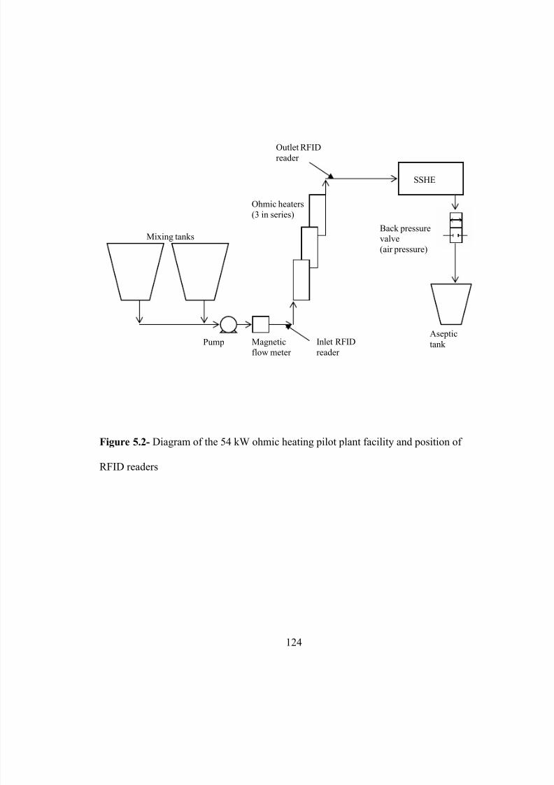
5/9/2018 Sarang Sanjay S - slidepdf.com
http://slidepdf.com/reader/full/sarang-sanjay-s 142/170
Mixing tanks
Pump Magnetic
flow meter
Ohmic heaters
(3 in series)
SSHE
Back pressure
valve
(air pressure)
Aseptic
tank Inlet RFID
reader
Outlet RFID
reader
Figure 5.2- Diagram of the 54 kW ohmic heating pilot plant facility and position of
RFID readers
124
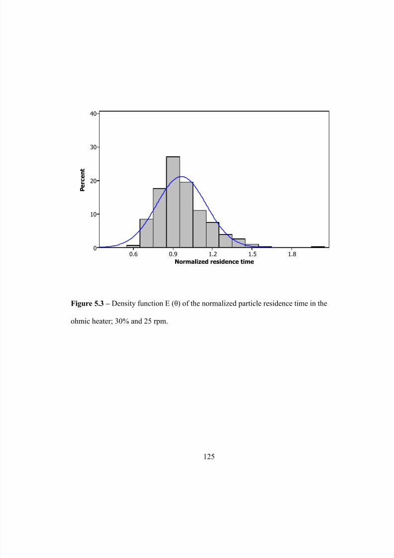
5/9/2018 Sarang Sanjay S - slidepdf.com
http://slidepdf.com/reader/full/sarang-sanjay-s 143/170
1.81.51.20.90.6
40
30
20
10
0
Normalized res idence t ime
P e r c e n t
Figure 5.3 – Density function E (θ) of the normalized particle residence time in the
ohmic heater; 30% and 25 rpm.
125
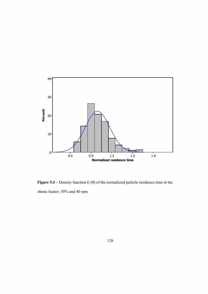
5/9/2018 Sarang Sanjay S - slidepdf.com
http://slidepdf.com/reader/full/sarang-sanjay-s 144/170
1.81.51.20.90.6
40
30
20
10
0
Normalized res idence t ime
P e r c e n t
Figure 5.4 – Density function E (θ) of the normalized particle residence time in the
ohmic heater; 30% and 40 rpm
126
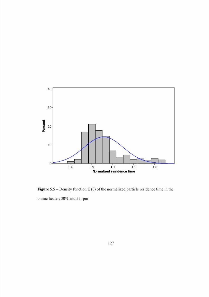
5/9/2018 Sarang Sanjay S - slidepdf.com
http://slidepdf.com/reader/full/sarang-sanjay-s 145/170
1.81.51.20.90.6
40
30
20
10
0
Normalized re sidence t ime
P e r c e n t
Figure 5.5 – Density function E (θ) of the normalized particle residence time in the
ohmic heater; 30% and 55 rpm
127
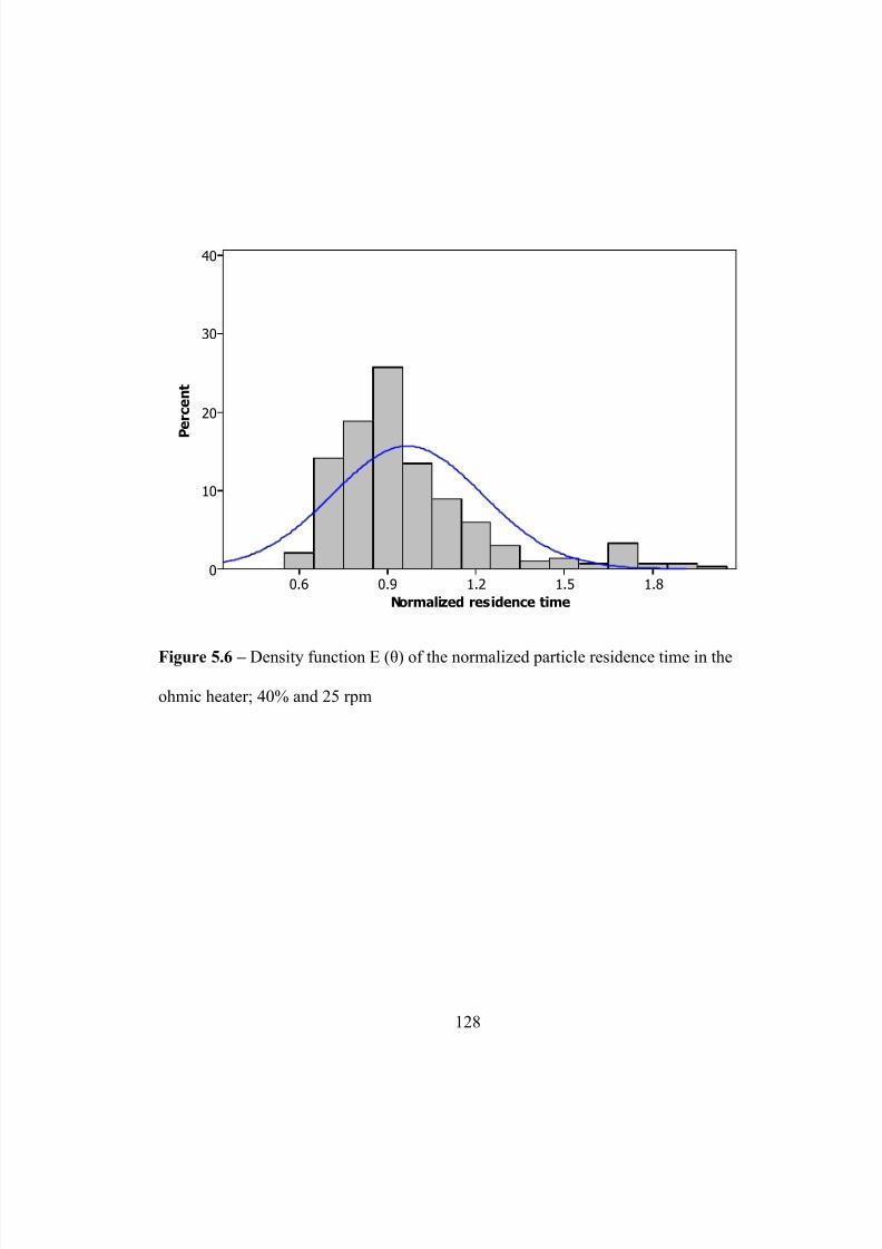
5/9/2018 Sarang Sanjay S - slidepdf.com
http://slidepdf.com/reader/full/sarang-sanjay-s 146/170
1.81.51.20.90.6
40
30
20
10
0
Normalized re sidence t ime
P
e r c e n t
Figure 5.6 – Density function E (θ) of the normalized particle residence time in the
ohmic heater; 40% and 25 rpm
128
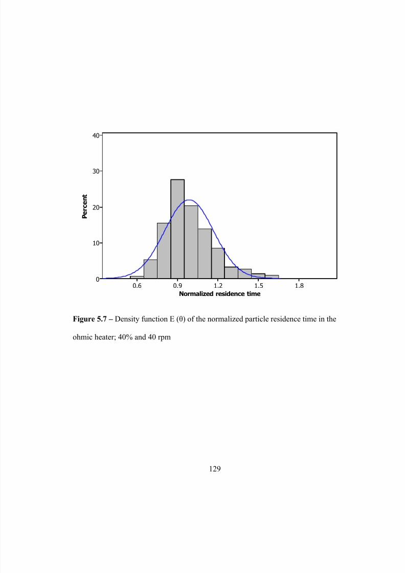
5/9/2018 Sarang Sanjay S - slidepdf.com
http://slidepdf.com/reader/full/sarang-sanjay-s 147/170
1.81.51.20.90.6
40
30
20
10
0
Normalized res idence t ime
P e r c e n
t
Figure 5.7 – Density function E (θ) of the normalized particle residence time in the
ohmic heater; 40% and 40 rpm
129
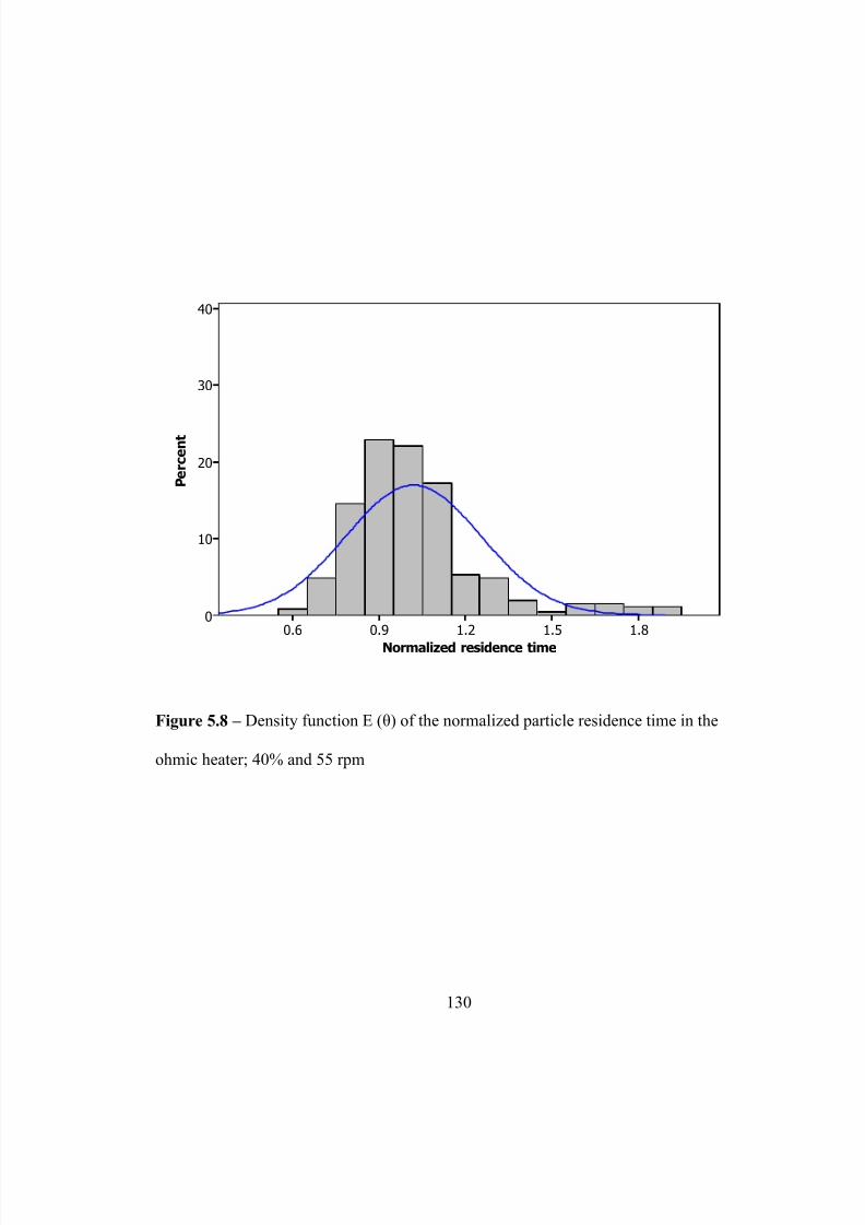
5/9/2018 Sarang Sanjay S - slidepdf.com
http://slidepdf.com/reader/full/sarang-sanjay-s 148/170
1.81.51.20.90.6
40
30
20
10
0
Normalized res idence t ime
P e r c e n t
Figure 5.8 – Density function E (θ) of the normalized particle residence time in the
ohmic heater; 40% and 55 rpm
130

5/9/2018 Sarang Sanjay S - slidepdf.com
http://slidepdf.com/reader/full/sarang-sanjay-s 149/170
1.81.51.20.90.6
40
30
20
10
0
Normalized res idence t ime
P e r c e n t
Figure 5.9 – Density function E (θ) of the normalized particle residence time in the
ohmic heater; 50% and 25 rpm
131
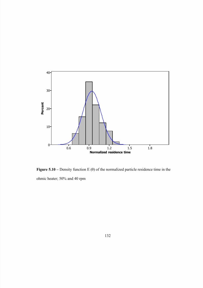
5/9/2018 Sarang Sanjay S - slidepdf.com
http://slidepdf.com/reader/full/sarang-sanjay-s 150/170
1.81.51.20.90.6
40
30
20
10
0
Normalized res idence t ime
P e r c e n t
Figure 5.10 – Density function E (θ) of the normalized particle residence time in the
ohmic heater; 50% and 40 rpm
132
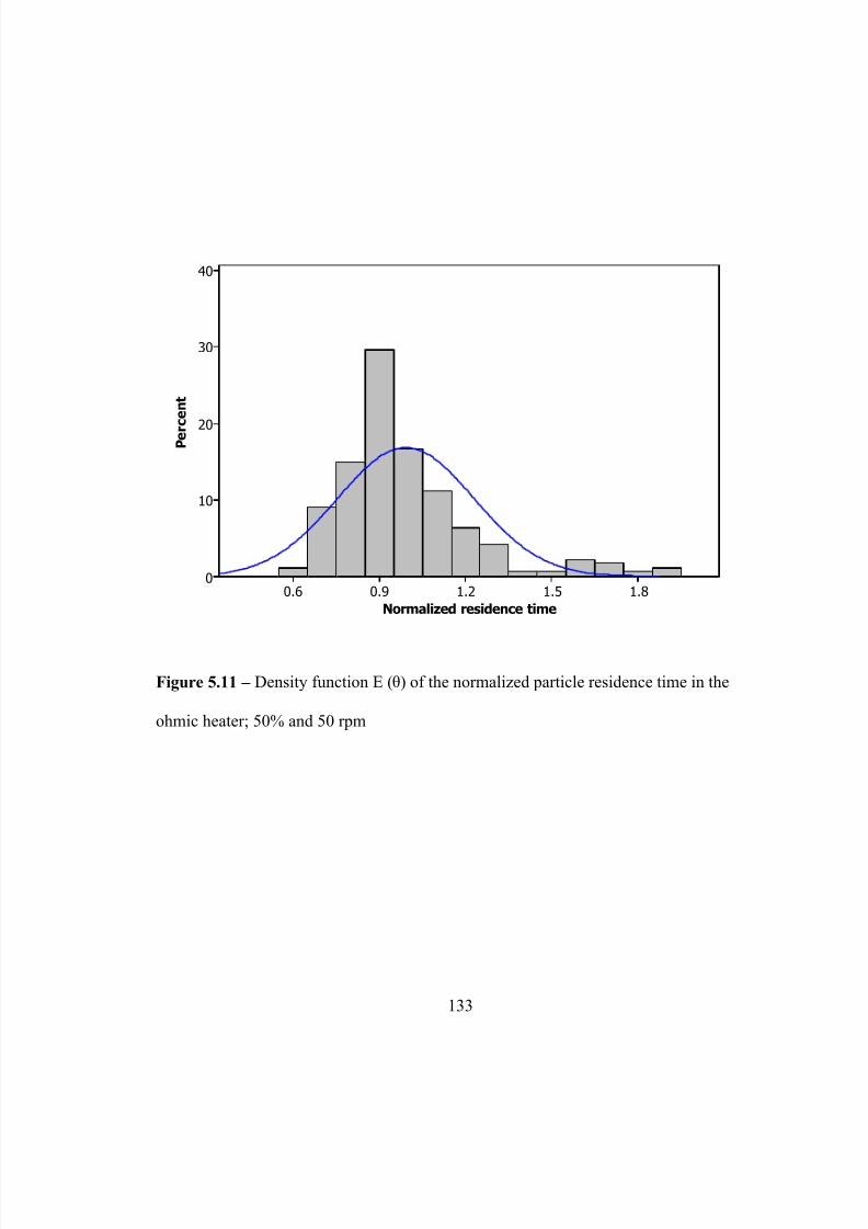
5/9/2018 Sarang Sanjay S - slidepdf.com
http://slidepdf.com/reader/full/sarang-sanjay-s 151/170
1.81.51.20.90.6
40
30
20
10
0
Normalized res idence t ime
P e r
c e n t
Figure 5.11 – Density function E (θ) of the normalized particle residence time in the
ohmic heater; 50% and 50 rpm
133
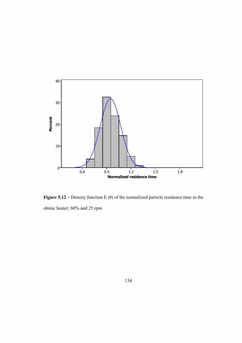
5/9/2018 Sarang Sanjay S - slidepdf.com
http://slidepdf.com/reader/full/sarang-sanjay-s 152/170
1.81.51.20.90.6
40
30
20
10
0
Normalized re sidence t ime
P e r c e n
t
Figure 5.12 – Density function E (θ) of the normalized particle residence time in the
ohmic heater; 60% and 25 rpm
134

5/9/2018 Sarang Sanjay S - slidepdf.com
http://slidepdf.com/reader/full/sarang-sanjay-s 153/170
1.81.51.20.90.6
40
30
20
10
0
Normalized re sidence t ime
P e r c e n t
Figure 5.13 – Density function E (θ) of the normalized particle residence time in the
ohmic heater; 60% and 40 rpm
135
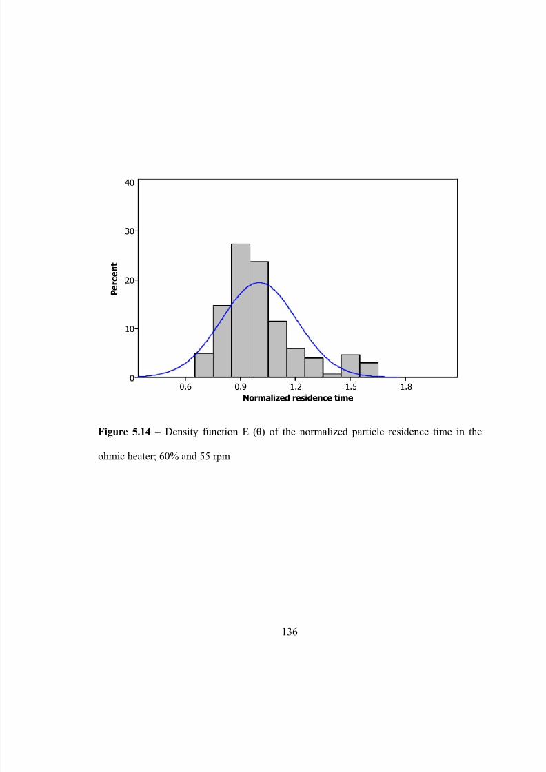
5/9/2018 Sarang Sanjay S - slidepdf.com
http://slidepdf.com/reader/full/sarang-sanjay-s 154/170
1.81.51.20.90.6
40
30
20
10
0
Normalized re sidence t ime
P e r c e n
t
Figure 5.14 – Density function E (θ) of the normalized particle residence time in the
ohmic heater; 60% and 55 rpm
136
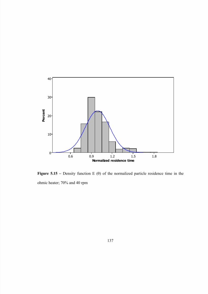
5/9/2018 Sarang Sanjay S - slidepdf.com
http://slidepdf.com/reader/full/sarang-sanjay-s 155/170
1.81.51.20.90.6
40
30
20
10
0
Normalized re sidence t ime
P e r c e n t
Figure 5.15 – Density function E (θ) of the normalized particle residence time in the
ohmic heater; 70% and 40 rpm
137
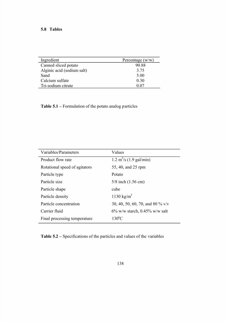
5/9/2018 Sarang Sanjay S - slidepdf.com
http://slidepdf.com/reader/full/sarang-sanjay-s 156/170
138
5.8 Tables
Ingredient Percentage (w/w)
Canned sliced potato 90.88
Alginic acid (sodium salt) 3.75Sand 5.00
Calcium sulfate 0.30
Tri-sodium citrate 0.07
Table 5.1 – Formulation of the potato analog particles
Variables/Parameters Values
Product flow rate 1.2 m3/s (1.9 gal/min)
Rotational speed of agitators 55, 40, and 25 rpmParticle type Potato
Particle size 5/8 inch (1.56 cm)
Particle shape cube
Particle density 1130 kg/m3
Particle concentration 30, 40, 50, 60, 70, and 80 % v/v
Carrier fluid 6% w/w starch, 0.45% w/w salt
Final processing temperature 130oC
Table 5.2 – Specifications of the particles and values of the variables
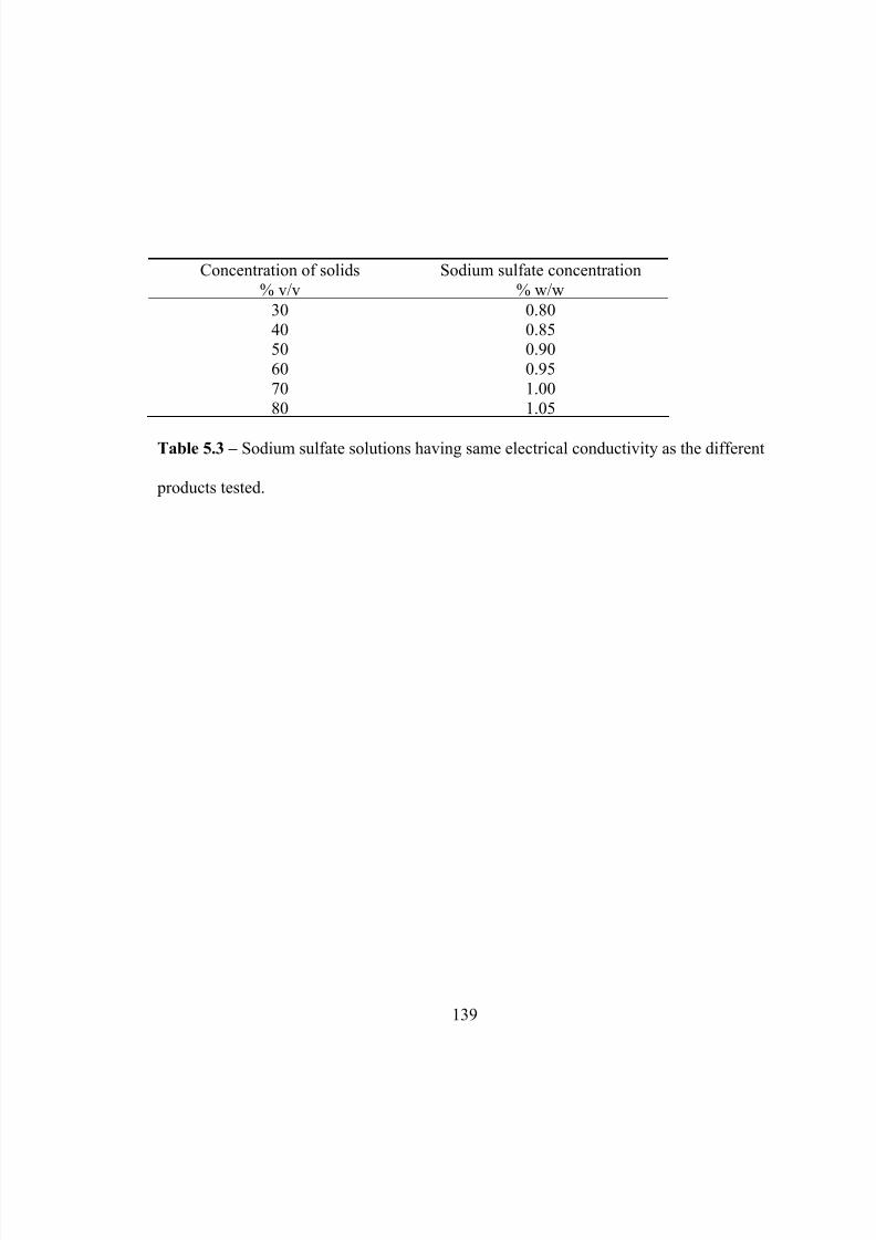
5/9/2018 Sarang Sanjay S - slidepdf.com
http://slidepdf.com/reader/full/sarang-sanjay-s 157/170
139
Concentration of solids
% v/v
Sodium sulfate concentration
% w/w
30 0.80
40 0.8550 0.90
60 0.95
70 1.00
80 1.05
Table 5.3 – Sodium sulfate solutions having same electrical conductivity as the different
products tested.

5/9/2018 Sarang Sanjay S - slidepdf.com
http://slidepdf.com/reader/full/sarang-sanjay-s 158/170
140
Rotational speed of agitators (rpm)Concentration of
solids (% v/v) 25 40 5530 59 64 60
40 58 59 59
50 61 63 6060 64 66 66
70 - 66 -
80 - - -
Table 5.4 - Minimum particle residence time in seconds - the effect of concentration of
solids and the rotational speed of the agitators
Rotational speed of agitators (rpm)Concentration of
solids (% v/v) 25 40 55
30 0.628 0.681 0.638
40 0.617 0.628 0.628
50 0.649 0.670 0.63860 0.681 0.702 0.702
70 - 0.702 -80 - - -
Table 5.5 - Minimum normalized particle residence time (MNNPRT) based on the
product mean residence time of 94 s - the effect of concentration of solids and the
rotational speed of the agitators
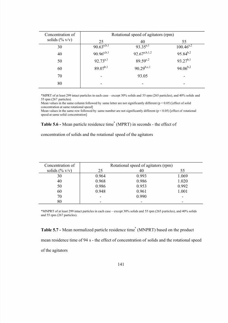
5/9/2018 Sarang Sanjay S - slidepdf.com
http://slidepdf.com/reader/full/sarang-sanjay-s 159/170
141
Rotational speed of agitators (rpm)Concentration of
solids (% v/v) 25 40 55
30 90.63a,b,1
93.35a,1
100.46a,2
40 90.96
a,b,1
92.67
a,b,1,2
95.84
b,2
50 92.73a,1
89.59c,2
93.27 b,1
60 89.07 b,1
90.29 b,c,1
94.06 b,2
70 - 93.05 -
80 - - -
*MPRT of at least 299 intact particles in each case – except 30% solids and 55 rpm (265 particles), and 40% solids and55 rpm (267 particles).Mean values in the same column followed by same letter are not significantly different (p < 0.05) [effect of solid
concentration at same rotational speed]Mean values in the same row followed by same number are not significantly different (p < 0.05) [effect of rotationalspeed at same solid concentration]
Table 5.6 - Mean particle residence time*
(MPRT) in seconds - the effect of
concentration of solids and the rotational speed of the agitators
Rotational speed of agitators (rpm)Concentration of
solids (% v/v) 25 40 5530 0.964 0.993 1.069
40 0.968 0.986 1.02050 0.986 0.953 0.992
60 0.948 0.961 1.001
70 - 0.990 -80 - - -
*MNPRT of at least 299 intact particles in each case – except 30% solids and 55 rpm (265 particles), and 40% solids
and 55 rpm (267 particles).
Table 5.7 - Mean normalized particle residence time*
(MNPRT) based on the product
mean residence time of 94 s - the effect of concentration of solids and the rotational speed
of the agitators
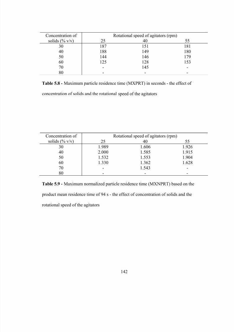
5/9/2018 Sarang Sanjay S - slidepdf.com
http://slidepdf.com/reader/full/sarang-sanjay-s 160/170
142
Rotational speed of agitators (rpm)Concentration of
solids (% v/v) 25 40 55
30 187 151 181
40 188 149 180
50 144 146 17960 125 128 15370 - 145 -
80 - - -
Table 5.8 - Maximum particle residence time (MXPRT) in seconds - the effect of
concentration of solids and the rotational speed of the agitators
Rotational speed of agitators (rpm)Concentration of solids (% v/v) 25 40 55
30 1.989 1.606 1.926
40 2.000 1.585 1.915
50 1.532 1.553 1.90460 1.330 1.362 1.628
70 - 1.543 -
80 - - -
Table 5.9 - Maximum normalized particle residence time (MXNPRT) based on the
product mean residence time of 94 s - the effect of concentration of solids and the
rotational speed of the agitators
5/9/2018 Sarang Sanjay S - slidepdf.com
http://slidepdf.com/reader/full/sarang-sanjay-s 161/170
143
CHAPTER 6
CONCLUSIONS
Ohmic heating offers an attractive alternative for continuous sterilization of foods
containing particulates because it heats simultaneously both the phases of the liquid-
particulate mixtures by internal energy generation. The critical property affecting energy
generation is the electrical conductivity of the food material. Electrical conductivity of
the selected solid foods increased linearly with temperature. Fruits were less conductive
than meat samples. Lower electrical conductivity was observed for porous materials like
apples. Lean muscle cuts were much more conductive compared to the separable fat.
Within the lean muscle cuts no relationship could be observed between the measured
electrical conductivity and the lean muscle fat content. Marbling (fat distribution) may be
the important factor affecting the electrical conductivity in lean muscle cuts.
In low-acid foods containing solid particulates like chicken chowmein the sauce
was more conductive than all the solid components. By blanching the solids in highly
conductive sauce it was possible to increase their ionic content and hence their electrical
conductivity. Product containing pretreated solids heated more uniformly during ohmic
heating. Sensory test results suggested that the blanching pretreatment did not
compromise the quality of the product. Following pretreatment, it may be possible to
5/9/2018 Sarang Sanjay S - slidepdf.com
http://slidepdf.com/reader/full/sarang-sanjay-s 162/170
144
uniformly heat the entire product during ohmic heating, thus, preventing thermal abuse
and improving the product quality.
Fick’s law can be used to describe sodium chloride diffusion in vegetable tissues
like Chinese water chestnut (CWC). The apparent diffusion coefficient increased
significantly with temperature. Simulation studies showed that after blanching the CWC
disc for 90 s (which was the blanching time required to match its conductivity to that of
the sauce), salt diffused only to the small depth from the surface and equilibration time is
much higher. So even though concentration and electrical conductivity is not uniformly
distributed throughout the solid it is possible to increase the overall ionic content and
electrical conductivity of the solid and heat it more rapidly during ohmic heating.
Residence time distribution (RTD) studies is necessary for the determination of
the fastest-moving particle for food safety consideration, and the determination of the
average and slowest-moving particle for food quality consideration. The residence times
and RTD of solid potato particles in starch solution were determined using Radio
Frequency Identification (RFID) technique. The effect of solid concentration and the
rotation speed of the agitators on the RTD were studied. Mean particle residence time
increased with the rotational speed, and no particular relationship was observed between
the measured mean particle residence time and the solid concentration. The velocity of
the fastest particle was 1.62 times the bulk mean product velocity which is important for
food safety design considerations.
5/9/2018 Sarang Sanjay S - slidepdf.com
http://slidepdf.com/reader/full/sarang-sanjay-s 163/170
145
LIST OF REFERENCES
Alhamdan, A. M. & Sastry, S. K. (1997). Residence time distribution of food and
simulated particles in a holding tube. Journal of Food Engineering, 34, 271–292.
Alhamdan, A. M. & Sastry, S. K., (1998) Residence time distribution of food and
simulated particles in a model horizontal swept-surface heat exchanger. Journal of
Food Process Engineering, 21, 145–180.
de Alwis, A. A. P., Halden, K. & Fryer, P. J. (1989). Shape and conductivity effects in
the ohmic heating of foods. Chemical Engineering Research, 67, 1547-1559
de Alwis, A. A. P. & Fryer, P. J. (1990). A finite element analysis of heat generation and
transfer during ohmic heating of food. Chemical Engineering Science, 45 (6), 1547-1559
Bean, E. C., Rasor, J. P., & Porter, G.C. (1960). Changes in electrical conductivities of avocados during ripening. Year Book of Californian Avocado Society, 44, 75–78.
Bhuptani, M. & Moradpour, S. (2005) RFID field guide: deploying radio frequencyidentification systems. Sun Microsystems/Prentice Hall PTR, Upper Saddle River, NJ.
Brown, K. L., Ayers, C. A., Gaze, J. E. & Newman, M. E. (1987). Thermal destruction of
bacterial spores immobilized in food/alginate particles. Food Microbiology, 1, 187.
Castro, I., Teixeira, J. A., Salengke, S., Sastry, S. K., & Vicente, A. A. (2003). Theinfluence of field strength, sugar and solid content on electrical conductivity of
strawberry products. Journal of Food Process Engineering, 26, 17-29.
Castro, I., Teixeira, J. A., Salengke, S., Sastry, S. K. & Vicente, A. A. (2004). Ohmic
heating of strawberry products: electrical conductivity measurements and ascorbicacid degradation kinetics. Innovative Food Science and Engineering Technologies, 5,27-36.
Chandarana, D. I. & Unverferth, J. A. (1996). Residence time distribution of particulate
foods at aseptic processing temperatures. Journal of Food Engineering 28, 349–360.
5/9/2018 Sarang Sanjay S - slidepdf.com
http://slidepdf.com/reader/full/sarang-sanjay-s 164/170
146
Del Valle, F. R., & Nickerson, J. T. R. (1967). Studies on salting and drying fish. 1.
Equilibrium considerations in salting. Journal of Food Science, 32, 173-179.
Del Valle, F. R., & Nickerson, J. T. R. (1967). Studies on salting and drying fish. 2.
Dynamic aspects of the salting of fish. Journal of Food Science, 218-224.
DiGeronimo, M., Garthright, W. & Larkin J. (1997). Statistical design and analysis. Food Technology 51(10), 52–54.
Drusas, A., & Vagenas, G. K. (1988). Diffusion of sodium chloride in green olives.
Journal of Food Engineering , 7, 211-222.
Dussap, G., & Gros, J. B. (1980). Diffusion sorption model for salt in pork and beef
muscle. In, P. Linko, Y. Malkki, J. Olkku, & J. Laringkari (Eds), Food Process Engineering (pp. 407-411). Applied Science Publishers, London.
Dutta, B. & Sastry, S. K. (1990). Velocity distribution of food particle suspensions inholding tube flow: experimental and modeling studies on average particle velocities. Journal of Food Science, 55 (5), 1448-1453.
Dutta, B. & Sastry, S. K. (1990). Velocity distribution of food particle suspensions in
holding tube flow: distribution characteristics and faster-particle velocities. Journal of
Food Science, 55 (6), 703-1710.
Fryer, P. J., deAlwis, A. A. P., Koury, E., Stapley, A. G. F. & Zhang, L. (1993). Ohmic processing of solid-liquid mixtures: heat generation and convection effects. Journal of Food Engineering, 18, 101-125.
Grabowski, P. P., Dan, G. & Parker, E. M. (1993). Method and apparatus for monitoring
continuous cooking process based on particulate residence time. U.S. Patent No.5,261,282.
Halden, K., de Alwis, A. A. P., & Fryer, P.J. (1990). Changes in the electrical
conductivity of foods during ohmic heating. International Journal of Food Science
and Technology, 25(1), 9–25.
Heinrich, C. E. (2005) RFID and beyond: Growing your business through real world
awareness. Wiley, Indianapolis, IN.
Icer, F., & Ilicali, C. (2005). Temperature dependent electrical conductivities of fruit purees during ohmic heating. Food Research International, 38, 1135-1142.
Khalaf, W. G. & Sastry, S. K. (1996). Effect of fluid viscosity on the ohmic heating rate
of solid-liquid mixtures. Journal of Food Engineering, 27, 125-158.
5/9/2018 Sarang Sanjay S - slidepdf.com
http://slidepdf.com/reader/full/sarang-sanjay-s 165/170
147
Kim, H. J., Choi, Y. M., Yang, C. S., Taub, I. A., Tempest, P., Skudder, P., Tucker, G. &
Parrott, D. L. (1996). Validation of ohmic heating for quality enhancement of food products. Food Technology, 253-262.
Kim, S. H., Kim, G. T., Park, J. Y. Cho, M. G., & Han, B. H. (1996). A study on the
ohmic heating of viscous food. Foods and Biotechnology, 5(4), 274-279.
Kim, H. J. & Taub, I. A. (1993). Intrinsic chemical markers for aseptic processing of
particulate foods. Food Technology, 47 (1), 91–97.
Klockeman, D. M., Pressey, R., & Jen, J. J. (1991). Characterization of cell wall
polysaccharides of jicama ( Pachyrrhizus erosus) and Chinese water chestnut( Eleocharis dulcis). Journal of Food Biochemistry, 15, 317-329
Larkin, J. W., & Spinak, S. H. (1996). Safety considerations of ohmically heated,aseptically processed, multiphase low-acid food products. Food Technology, 242-
245.
Lee, J. H. & Singh, R. K. (1991). Particle residence time distribution in a modelhorizontal scraped-surface heat exchanger. Journal of Food Process Engineering, 14,
125-146.
Lima, M., & Sastry, S. K. (1999). The effect of ohmic heating frequency on hot-air
drying rate and juice yield. Journal of Food Engineering, 41, 115-119.
Liu, H. (1992). A kinetic study of salt diffusion in potato at high temperature. International Journal of Food Science and Technology, 27, 443-455.
Manavel, J. E., Powell, R. L., McCarthy, M. & McCarthy, K. L. (1993). Magneticresonance imaging of multiphase systems. Butterworth-Heinemann, Boston.
Marcotte, M., Trigui, M., Tatibouet, J. & Ramaswamy, H. S. (2000). An ultrasonic
method for assessing the residence time distribution of particulate foods during ohmic
heating. Journal of Food Science: Food Engineering and Physical Properties 65 (7),1180-1186
Mavroudis, N. E., Dejmek, P., & Sjoholm, I. (2004). Studies on some raw materialcharacteristics in different Swedish apple varieties. Journal of Food Engineering , 62,
121-129.
McCoy, S., Zuritz, C. & Sastry, S. K. (1987). Residence time distribution of simulated
food particles in a holding tube. ASAE Paper No. 87-6536. ASAE, St. Joseph, MI.
Mitchell, F. R. G. & deAlwis, A. A. P. (1989). Electrical conductivity meter for food particles. Journal of Physics E , 22, 554-556.
5/9/2018 Sarang Sanjay S - slidepdf.com
http://slidepdf.com/reader/full/sarang-sanjay-s 166/170
148
Mudahar, G. S., & Jen, J. J. (1991). Texture of raw and canned jicama ( Pachyrrhizus
tuberosus) and Chinese water chestnut ( Eleocharis dulcis). Journal of Food Science,
56 (4), 977-980.
Orangi, S., Sastry, S. K. & Li, Q. (1997). A numerical investigation of electroconductiveheating in solid-liquid mixtures. International Journal of Heat and Mass Transfer, 41
(14), 2211-2220.
Palaniappan, S. & Sastry, S. (1991). Electrical conductivities of selected solid foods
during ohmic heating. Journal of Food Process Engineering , 14, 221-136
Palaniappan, S. & Sastry, S. (2002). Ohmic heating. In Control of Foodborne
Microorganisms, Eds. V. K. Juneja & J. N. Sofos. New York: Marcel Dekker, 451-
460.
Palaniappan, S., & Sastry, S. (2002). Ohmic heating. In V. K. Juneja & J. N. Sofos (Eds) Control of Foodborne Microorganisms, (pp. 451-460). New York: Marcel Dekker.
Palaniappan, S., & Sizer, C. E. (1997). Aseptic process validation for food containing
particulates. Food Technology, 51(8), 60-68.
Paret, D. (2005) RFID and contactless smart card applications. Wiley, Hoboken, NJ.
Parker, M. L., & Waldron K. W. (1995). Texture of Chinese water chestnut: involvementof cell wall phenolics. Journal of the Science of Food and Agriculture, 68, 337-346.
Parker, C. C., Parker, M. L., Smith, A. C., & Waldron, K. W. (2003). Thermal stability of texture in Chinese water chestnut may be dependent on 8, 8- Diferulic acid
(Aryltetralyn form). Journal of Agricultural and Food Chemistry, 51, 2034-2039.
Rahman, M. S. (1999). In Rahman, M. S., (Ed.), Handbook of Food Preservation; (pp.
521-532). Dekker: New York.
Rahman, M. S., Al-Zakwani, I., & Guizani, N. (2005). Pore formation in apple during air-
drying as a function of temperature: porosity and pore-size distribution. Journal of theScience of Food and Agriculture, 85, 979-989.
Ramaswamy, H. S., Abdelrahim, K. A., Simpson, B. K. & Smith, J. P. (1995). Residencetime distribution (RTD) in aseptic processing of particulate foods: a review. Food Res
Int 28(3), 291–310.
Ruhlman, K. T., Jin, Z. T. & Zhang, Q. H. (2001) Physical properties of liquid foods for
pulsed electric field treatment. In Pulsed Electric Fields in Food Processing. Eds.
5/9/2018 Sarang Sanjay S - slidepdf.com
http://slidepdf.com/reader/full/sarang-sanjay-s 167/170
149
Barbosa-Canovas, G. V. & Zhang, Q. H. Technomic Publishing Co., Lancaster, PA.,
45-56.
de Ruyter, P. W. & Brunet, R. (1973) Estimation of process conditions for the continuous
sterilization of foods containing particulates. Food Technology, 27(7), 44-51.
Saif, S. M. H., Lan, Y., Wang, S., & Garcia, S. (2004). Electrical resistivity of goat meat. International Journal of Food Properties, 7(3), 463-471.
Salengke, S. & Sastry, S. K. (1995). Residence time distribution of cylindrical particles in
a curved section of a holding tube: the effect of particle size and flow rate. Journal of Food Engineering, 18, 363-381.
Salengke, S. & Sastry, S. K. (1996). Residence time distribution of cylindrical particles in
a curved section of a holding tube: the effect of particle concentration and bend radiusof curvature. Journal of Food Engineering, 27, 159–176.
Salengke, S., & Sastry, S. K. (2007). Experimental investigation of ohmic heating of
solid-liquid mixtures under worst-case heating scenarios. Journal of Food
Engineering, 83 (3), 324-336.
Salengke, S., & Sastry, S. K. (2007). Models for ohmic heating of solid-liquid mixturesunder worst-case heating scenarios. Journal of Food Engineering, 83 (3), 337-355.
Sancho, M. F. & Rao, M. A. (1991). Residence time distribution in a holding tube. Journal of Food Engineering, 15, 1-19.
Sasson, A., & Monselise, A. P. (1977). Electrical conductivity of ’shamouti’ orange peelduring fruit growth and postharvest senescence. Journal of American Society: Horticulture Science, 102(2), 142–144.
Sastry, S. K. (1992). A model for heating of liquid-particle mixtures in a continuous flow
ohmic heater. Journal of Food Process Engineering, 15, 263-278
Sastry S. K. (1997). Measuring residence time and modeling the system. Food
Technology 51(10), 44–48.
Sastry, S. K. & Cornelius, B. D. (2002). Aseptic processing of foods containing solid
particulates. Jon Wiley and Sons, Inc. New York.
Sastry, S. K. & Palaniappan, S. (1992). Ohmic heating of liquid-particle mixtures. Food
Technology, 46 (12), 64-67.

5/9/2018 Sarang Sanjay S - slidepdf.com
http://slidepdf.com/reader/full/sarang-sanjay-s 168/170
150
Sastry, S. K. & Palaniappan, S. (1992). Influence of particle orientation on the effective
electrical resistance and ohmic heating rate of a liquid-particle mixture Journal of
Food Process Engineering, 15, 213-227.
Sastry, S. K. & Palaniappan, S. (1992). Mathematical modeling and experimental studies
on ohmic heating of liquid-particle mixtures in a static heater. Journal of Food Process Engineering, 15, 241-261.
Sastry, S. K. & Li, Q. (1996). Modeling the ohmic heating of foods. Food Technology. 50(5), 246-248.
Sastry, S. K. & Salengke, S. (1998). Ohmic heating of solid-liquid mixtures: Acomparison of mathematical models under worst-case heating conditions. Journal of
Food Process Engineering, 21, 441-458.
Segner, W. P., Ragusa, T. J., Marcus, C. L. & Soutter, E. A. (1989). Biological evaluation
of a heat transfer simulation for sterilizing low-acid large particulate foods for aseptic packaging. Journal of Food Processing and Preservation, 13, 257–274.
Sensoy, I. (2002) Ohmic and moderate electric field treatment of foods: studies on heat
transfer modeling, blanching, drying, rehydration and extraction. Thesis (PhD) Ohio
State University, 2002.
Shirsat, N., Lyng, J. G., Brunton, N. P., & McKenna, B. (2004). Ohmic processing:
Electrical conductivities of pork cuts. Meat Science, 67, 507-514.
Singh, R. P. and Heldman, D. R. (1984) Introduction to Food Engineering Academic
Press, Inc., San Diego, CA
Skoog, D. F., & West, D. M. (1976). Fundamentals of Analytical Chemistry. (pp. 232-233) Holt, Rinehart and Winston, New York.
Swartzel, K. R., Ganeshan, S. G., Kuehn, R. T., Hamaker, R. W. & Sadeghi, F. (1991).
Thermal memory cell and thermal system evaluation. U.S. Patent No. 5,021,981.
Tang, H., Belton, P. S., Ng, A., & Ryden, P. (1999).13
C MAS NMR studies of the effects
of hydration on the cell walls of potatoes and Chinese water chestnuts. Journal of
Agricultural and Food Chemistry, 47, 510-517.
Tucker, G. S. & Withers, P. M. (1994). Determination of residence time distribution of nonsettling food particulates in viscous food carrier fluids using Hall effect sensors.
Journal of Food Process Engineering, 17, 401–422.
5/9/2018 Sarang Sanjay S - slidepdf.com
http://slidepdf.com/reader/full/sarang-sanjay-s 169/170
151
Tulsiyan, P., Sarang, S., & Sastry, S. K. (2007). Electrical conductivity of
multicomponent systems during ohmic heating. International Journal of Food
Properties, (accepted).
Tulsiyan, P., Sarang, S., & Sastry, S. K. (2007). Radio Frequency Identification:
Residence Time Distribution of a Multicomponent System inside Ohmic Heater. Journal of Food Science, (submitted).
U.S. Department of Agriculture, Agricultural Research Service. (2005). USDA NutrientDatabase for Standard Reference, Release 18. Nutrient Data Laboratory Home Page,
http://www.nal.usda.gov/fnic/foodcomp
Wang, W. & Sastry, S. (1993 a). Salt diffusion into vegetable tissue as a pretreatment for
ohmic heating: electrical conductivity profiles and vacuum infusion studies. Journal of Food Engineering, 20, 299-309.
Wang, W. & Sastry, S. (1993 b). Salt diffusion into vegetable tissue as a pretreatment for ohmic heating: determination of parameters and mathematical model verification. Journal of Food Engineering, 20, 311-323.
Wang, W. & Sastry, S.K. (1997). Changes in electrical conductivity of selected
vegetables during multiple thermal treatments. Journal of Food Process Engineering , 20, 499-516.
Wang, W. C., & Sastry, S. K. (2000). Effects of thermal and electrothermal pretreatmentson hot air drying rate of vegetable tissue. Journal of Food Process Engineering , 23,
299-219.
Wang, W. C., & Sastry, S. K. (2002). Effects of moderate electrothermal treatments on
juice yield from cellular tissue. Innovative Food Science and Emerging Technologies,3(4), 371-377.
Williams, W. J. (1979). Handbook of Anion Determination. (pp. 297-301) Butterworths,
London.
Wistreich, H. E., Morse, R. E., & Kenyon, L. J. (1960) Curing of ham: a study of sodium
chloride accumulation. II: Combined effects of time, solution concentration andsolution volume. Food Technology, 14, 549-551.
Wood, F. W. (1966). The diffusion of salt in pork muscle and fat tissue. Journal of the
Science of Food and Agriculture, 17, 138-140.
Zhang, L. & Fryer, P. J. (1993). Models for the electrical heating of solid-liquid mixtures.Chemical Engineering Science. 48, 633-643
5/9/2018 Sarang Sanjay S - slidepdf.com
http://slidepdf.com/reader/full/sarang-sanjay-s 170/170
152
Zhong, T., & Lima, M. (2003). The effect of ohmic heating on vacuum drying rate of
sweet potato tissue. Bioresource Technology, 87, 215-220.
Zitoun, K. B., Sastry, S. K. & Guezennec, Y. (2001). Investigation of three dimensional
interstitial velocity, solids motion , and orientation in solid-liquid flow using particle
tracking velocimetry. International Journal of Multiphase Flow, 27, 1397–1414.