Saqib Paper
21
arXiv:1402.2731v2 [gr-qc] 10 Nov 2014 Dynamics of a Charged Particle Around a Slowly Rotating Kerr Black Hole Immersed in Magnetic Field Saqib Hussain, 1, * Ibrar Hussain, 2, † and Mubasher Jamil 1, ‡ 1 School of Natural Sciences (SNS), National University of Science and Technology (NUST), H-12, Islamabad, Pakistan 2 School of Electrical Engineering and Computer Science (SEECS), National University of Sciences and Technology (NUST), H-12, Islamabad, Pakistan Abstract: The dynamics of a charged particle moving around a slowly rotating Kerr black hole in the presence of an external magnetic field is investigated. We are interested to explore the conditions under which the charged particle can escape from the gravitational field of the black hole after colliding with another particle. The escape velocity of the charged particle in the innermost stable circular orbit is calculated. The effective potential and escape velocity of the charged particle with angular momentum in the presence of magnetic field is analyzed. This work serves as an extension of a preceding paper dealing with the Schwarzschild black hole [Zahrani et al, Phys. Rev. D 87, 084043 (2013)]. * Electronic address: [email protected] † Electronic address: [email protected] ‡ Electronic address: [email protected] , [email protected]
description
Dynamics of a Charged Particle Around a Slowly Rotating Kerr Black HoleImmersed in Magnetic Field
Transcript of Saqib Paper
arX
iv:1
402.
2731
v2 [
gr-q
c] 1
0 N
ov 2
014
Dynamics of a Charged Particle Around a Slowly Rotating Kerr Black Hole
Immersed in Magnetic Field
Saqib Hussain,1, ∗ Ibrar Hussain,2, † and Mubasher Jamil1, ‡
1School of Natural Sciences (SNS), National University of
Science and Technology (NUST), H-12, Islamabad, Pakistan
2School of Electrical Engineering and Computer Science (SEECS),
National University of Sciences and Technology (NUST), H-12, Islamabad, Pakistan
Abstract: The dynamics of a charged particle moving around a slowly rotating Kerr black
hole in the presence of an external magnetic field is investigated. We are interested to explore
the conditions under which the charged particle can escape from the gravitational field of the
black hole after colliding with another particle. The escape velocity of the charged particle in
the innermost stable circular orbit is calculated. The effective potential and escape velocity
of the charged particle with angular momentum in the presence of magnetic field is analyzed.
This work serves as an extension of a preceding paper dealing with the Schwarzschild black
hole [Zahrani et al, Phys. Rev. D 87, 084043 (2013)].
∗Electronic address: [email protected]†Electronic address: [email protected]‡Electronic address: [email protected] , [email protected]
2
I. INTRODUCTION
The dynamics of particles (massive or massless, charged or neutral) around a black hole is
among the most important and interesting problems of black hole astrophysics. These studies not
only help us to understand the geometrical structure of spacetimes but also shed light on the high
energy phenomenon occurring near the black hole such as formation of jets (which involve particles
to escape) and accretion disks (particles orbiting in circular orbits). Due to the presence of strong
gravitational and electromagnetic fields, charged particles in general do not follow stable orbits
and inter-particle collisions are most common. The aftermath of these collisions among numerous
particles lead to various interesting astrophysical phenomenon.
There are numerous astrophysical evidence that magnetic field might be present in the nearby
surrounding of black holes [1, 2] which support the large scale jets. These jets are most likely the
source of cosmic rays and high energy particles coming from nearby galaxies. The origin of this
magnetic field is the probable existence of plasma in the vicinity of a black hole in the form of an
accretion disk or a charged gas cloud [3, 4]. The relativistic motion of particles in the conducting
matter in the accretion disk can generate the regular magnetic field inside the disk. Therefore near
the event horizon of a black hole, it is expected that there exists much strong magnetic field. To
an approximation, it is presumed that this field does not effect the geometry of the black hole but
it does effect the motion of the charged particles moving around the black hole [5, 6].
More importantly, a rotating black hole may provide sufficient energy to the particle moving
around it due to which the particle may escape to spatial infinity. This physical effect appears to
play a crucial role in the ejection of high energy particles from accretion disks around black holes.
In the process of ejection of high energy particles, besides the rotation of black hole, the magnetic
field plays an important role [7, 8]. Note that if the black hole is carrying electric charge producing
the static electric field (also called Coulomb field), then the mere rotation of black hole itself
induces the magnetic field. Acceleration of the particle by the black hole is generally explained in
[9]. Other interesting processes around black holes may include evaporation and phantom energy
accretion onto black holes [10].
During the motion of a charged particle around a magnetized black hole, it remains under the
influence of both gravitational and electromagnetic forces which makes the situation complicated
[11, 12]. In the present article, it is considered that a charged particle is orbiting in the innermost
stable circular orbit (ISCO) of a slowly rotating Kerr black hole and is suddenly hit by a radially
incoming neutral particle. The aftermath of collision will depend on the energy of the incoming

3
particle which may result one of the three possible outcomes: charged particle may escape to
infinity; being captured by the black hole or keep orbiting in ISCO. However predicting the nature
of outcome is compounded by the facts that particle is charged and interacts with the magnetic field
and is frame dragged by the Kerr black hole. It should be noted that the present work is altogether
different from the BSW mechanism where two particles (with non-zero angular momentum and
high energies) arrive from spatial infinity and collide near the event horizon to generate surplus
energy in the center of mass frame [13]. In literature, motion of charged particles in ISCO around
various black holes has been studied ([14] and see therein).
Here we consider a slowly rotating Kerr black hole which is surrounded by an axially symmetric
magnetic field homogeneous at infinity. Almost similar problem was studied for weakly charged
rotating black holes in [15]. Their main conclusion is that, if the magnetic field is present than the
ISCO is located closer to the black hole horizon. In general, the effect of the black hole rotation on
the motion of a neutral particle is same as the effect of magnetic field on the motion of a charged
particle [16, 17].
To study the escape velocity of a particle from the vicinity of black hole, in this paper we
first consider a neutral particle moving around a slowly rotating Kerr black hole in the absence
of magnetic field and collides with another particle. For simplicity we consider the motion in
the equatorial plane only. Then we consider the same problem for a charged particle in the
presence of magnetic field. We focus under what circumstances the particle can escape from
the strong gravitational field to infinity. Magnetic field is homogeneous far from the black hole
and gravitational field is ignorable. Thus, far from the black hole charged particle moves in a
homogeneous magnetic field. If the magnetic field is absent then the equations of motion are
simple a little and can be solved analytically. When a particle moving in a non uniform magnetic
field in the absence of black hole its motion is chaotic [18, 19]. We are extending a previous work
[16] for the slowly rotating Kerr black hole.
The outline of the paper is as follows: In section II we explain our model and derive an expression
for escape velocity of the neutral particle. In section III we derive the equations of motion of the
charged particle moving around a slowly rotating weakly magnetized Kerr black hole. In section
IV we give the dimensionless form of the equations. Trajectories for escape energy and escape
velocity of the particle are discussed in section V and VI respectively and their graphs are given
in the appendix. Summery and conclusion are presented in section VII. Throughout we use sign
convention (+,−,−,−) and units where c = 1, G = 1.

4
II. ESCAPE VELOCITY FOR A NEUTRAL PARTICLE
We start with the simple case of calculating the escape velocity when the particle is neutral and
magnetic field is absent. The Kerr metric is given by [20]
ds2 =∆− a2 sin2 θ
ρ2dt2 +
4Mar sin2 θ
ρ2dφdt− ρ2
∆dr2 − ρ2dθ2 − A sin2 θ
ρ2dφ2,
∆ ≡ r2 − 2Mr + a2, ρ2 ≡ r2 + a2 cos2 θ, A ≡ (r2 + a2)2 − a2∆sin2 θ, (1)
where M is the mass and a is the spin of the black hole and interpreted as the angular momentum
per unit mass of the black hole a = LM. The horizons of Kerr metric are obtained by solving
∆(r) = r2 + a2 − 2Mr = 0. (2)
From the above equation we get two values of r:
r+ = M +√
M2 − a2, r− = M −√
M2 − a2. (3)
Note that ∆ > 0 for r > r+ and r < r− and ∆ < 0 for r− < r < r+ [23]. The region r = r+
represents the event horizon while r− is termed as the Cauchy horizon. Further r = 0 and θ = π2
is the location of a curvature ring-like singularity in the Kerr spacetime.
In literature, slowly rotating Kerr black holes have been investigated for numerous astrophysical
processes including as retro-MACHOS [24], particle acceleration via BSW mechanism [25], thin
accretion disk and accretion rates [26], to list a few. Hence we consider the slowly rotating black
hole and neglect the terms involving a2. The line element in (1) becomes
ds2 = (1− rgr)dt2 +
4aM sin2 θ
rdφdt− 1
1− rgr
dr2 − r2dθ2 − r2 sin2 θdφ2. (4)
Here rg = 2M , is the gravitational radius of the slowly rotating Kerr black hole just like
Schwarzschild black hole (Note that for a slowly rotating Kerr and Schwarzschild black hole the
horizon occurs at r = rg ). Clearly the metric (4) is stationary but non-static since dt → −dt,
changes the signature of metric. The metric is also axially symmetric (invariance under dθ → −dθ).
In terms of Lagrangian mechanics (L = gµν xµxν), the t and φ coordinates are cyclic which
lead to two conserved quantities namely energy and angular momentum with the corresponding
Noether symmetry generators
ξ(t) = ξµ(t)∂µ =∂
∂t, ξ(φ) = ξµ(φ)∂µ =
∂
∂φ. (5)

5
This shows that the black hole metric is invariant under time translation and rotation around sym-
metry axis. The corresponding conserved quantities are the energy E per unit mass and azimuthal
angular momentum Lz per unit mass 1
t =r3E + aLzrgr2(r − rg)
,
φ =1
r2
(
argE(r − rg)
+Lz
sin2 θ
)
. (6)
From the astrophysical perspective, it is known that particles orbit a rotating black hole in the
equatorial plane [27]. Therefore we choose θ = π2 to get
t =r3E + aLzrgr2(r − rg)
,
φ =1
r2( argE(r − rg)
+ Lz
)
. (7)
Throughout in this paper the over dot represents differentiation with respect to proper time τ .
Using the normalization condition, uµuµ = 1, we get the equation of motion
r2 =(Er2 − aLz)
2
r4− r2 − rgr
r4(r2 + L2
z − 2aELz). (8)
At the turning points r = 0, the equation (8) is quadratic in E whose solution is
E =aLzrg ±
√
r5(r − rg) + L2z(r
4 − r3rg + a2r2g)
r3, (9)
which gives E = Veff, the effective potential. The condition r = 0 is termed as the turning point
because it gives the location at which an incoming particle turns around from the neighborhood
of the gravitating source [28]. As we are considering only the positive energy therefore we will
consider only the positive sign before the square root in equation (9) for all the further calculation.
Equations (8) and (9) hold for equatorial plane only. It can be seen from (9) that E → 1 for r → ∞.
Therefore the minimum energy for the particle to escape from the vicinity of black hole is 1.
Consider a particle in ISCO, where ro is the local minima (which is also the convolution point)
of the effective potential [23]. The corresponding energy and azimuthal angular momentum are
given by [23, 29] after neglecting terms which involving a2 we have
Lzo = ±
√rg
(
ro ± a√
2rgro
)
√
2ro − 3rg ∓ 2a√
2rgro
, (10)
1 Given a Lagrangian L = gµν xµxν , one can calculate the conserved quantities corresponding to cyclic coordinates
t and φ as ddτ
∂L
∂t= 0, and d
dτ∂L
∂φ= 0, yielding ∂L
∂t= E ≡ −pµξ
µ
(t)/m, and ∂L
∂φ= Lz ≡ pµξ
µ
(φ)/m. Solving these
equations simultaneously, one can obtain (6).

6
Eo =1− rg
r∓ a
r
√
rg2r
√
1− 3rg2r ∓ a
r
√
2rgr
. (11)
Now consider the particle in the ISCO which collides with another incoming particle. After collision
between these particles, three cases are possible for the motion of the particle: (i) bound motion
(ii) capture by the black hole (iii) escape to infinity. The result will depend on the collision process.
For small change in energy and momentum, orbit of the particle will be slightly perturbed. While
for large change in energy and angular momentum, the particle can either be captured by black
hole or escape to infinity.
After the collision particle should have new values of energy and momentum E , Lz and the
total angular momentum L2. We simplify the problem by applying the following conditions (i) the
azimuthal angular momentum is fixed (ii) initial radial velocity remains same after the collision.
Under these conditions only energy of the particle can determine its motion. After collision particle
acquires an escape velocity (v⊥) in orthogonal direction of the equatorial plane [21]. The square of
total angular momentum of the particle after collision is given by
L2 = r4θ2 + r4 sin2 θφ2. (12)
Putting the value of φ from equation (6) in equation (12) we have
L2 = r2v2⊥ + sin2 θ
(
argEor − rg
+Lzo
sin2 θ
)2
. (13)
Here we denote v ≡ −rθo. Note that L2 is not the integral of motion. It is conserved for a = 0 i.e.
in the spherically symmetric case. However now the metric is axially symmetric, therefore only
Lz component is conserved. In a flat spacetime, all three components Lx, Ly, Lz are conserved,
and so is the square of the total angular momentum. The angular momentum Lzo and energy Eoappearing in (13) are given by (10) and (11) which provide the necessary corrections due to spin
of the black hole.
From equations (9) and (13), the angular momentum and the energy of the particle after the
collision becomes
L2 = r2ov2⊥ +
(
argEoro − rg
+ Lzo
)2
, (14)
Enew =aLrg +
√
r5o(ro − rg) + L2(r4o − r3org + a2r2g)
r3o. (15)
These values of angular momentum and energy are greater than their values before the collision.
Physically it means that the energy of the particle exceeds its rest mass energy. We have mentioned

7
above all the orbits with Enew ≥ 1 are unbounded in the sense that particle escapes to infinity.
Conversely for Enew < 1, particle cannot escape to infinity (the orbits are always bounded).
Therefore particle escapes to infinity if Enew ≥ 1, or
v⊥ ≥ ±r(rg − r)(Lz(r − rg) + arg(Eo − 1)) +√
r2rg(r − rg)2(r3 + rg(a2 − r2 − 2a2Eo))r2(r − rg)2
. (16)
Particle escape condition is |v| ≥ v⊥ i.e. the magnitude of velocity should be greater than any
orthogonal velocity.
III. CHARGED PARTICLE AROUND THE SLOWLY ROTATING MAGNETIZED
KERR BLACK HOLE
Here we investigate the motion of a charged particle (electric charge q) in the presence of
magnetic field in the exterior of the slowly rotating Kerr black hole. The Killing equation is
�ξµ = 0, (17)
where ξµ is a Killing vector. Note that (17) follows from the result: a Killing vector in a vacuum
spacetime generates a solution of Maxwell equations i.e. Fµν = −2ξµ;ν . From Fµν;ν = 0, it follows
that −2ξµ;ν;ν = 0. Thus (17) coincides with the Maxwell equation for 4-potential Aµ in the Lorentz
gauge Aµ;µ = 0. The special choice for Aµ is [2, 15].
Aµ =(
aB, 0, 0, B2
)
, (18)
where B is the magnetic field strength. The 4-potential is invariant under the symmetries which
correspond to the Killing vectors, i.e.,
LξAµ = Aµ,νξν +Aνξ
ν,µ = 0. (19)
A magnetic field vector is defined as
Bµ = −1
2eµνλσFλσuν , (20)
where
eµνλσ =ǫµνλσ√−g
, ǫ0123 = 1, g = det(gµν). (21)
In (21) ǫµνλσ is the Levi Civita symbol and the Maxwell tensor is defined as
Fµν = Aν;µ −Aµ;ν . (22)

8
For a local observer at rest we have
uµ =( 1√
(1− rgr) +
4aM√
(1−rg
r)
r2 sin θ
, 0, 0,1
r sin θ√
(1 + 4aM
r2 sin θ
√
(1−rgr))
)
. (23)
From (20)− (23) we can obtain the components of magnetic field
Bµ = B(
0, cos θ( (1− rg
r)
√
(1− rgr) +
2rga√
(1−rg
r)
r2 sin θ
)
+rga sin θ cos θ
r
( (1− rgr)
r sin θ√
(1 +2rga
r2 sin θ
√
(1−rgr))
)
,
,− sin θ(1− rgr)
r
√
(1− rgr) +
2rga√
(1−rgr)
r2 sin θ
, 0)
. (24)
For the equatorial plane only, the third component of the magnetic field will survive. Hence
equation (24) becomes
Bµ = B(
0, 0,− (1− rgr)
r
√
(1− rgr) +
2rga√
(1−rgr)
r2
, 0)
. (25)
The Lagrangian of the particle of mass m and charge q moving in an external magnetic field in
a curved spacetime is [22]
L =1
2gµν x
µxν +qAµ
mxµ, (26)
and generalized 4-momentum of the particle is Pµ = muµ + qAµ. The constants of motion are
t =r3E + aLzrgr2(r − rg)
− 2aB,
φ =1
r2
(
argE(r − rg)
+Lz
sin2 θ
)
−B. (27)
For the equatorial plane θ = π2 the above integrals of motion become
t =r3E + aLzrgr2(r − rg)
− 2aB,
φ =1
r2( argE(r − rg)
+ Lz
)
−B. (28)
Here we denote
B ≡ qB2m
. (29)
After putting the value of t and φ and neglecting the terms involving a2, Eq. (26) yields
L =1
2r2(r − rg)2
[
4Br2Lz(rg − r) + L2z(rg − r) +
r2(
Brg(3Br2 + 2aE)r(E2 − 3B2r2 − r2))
]
. (30)

9
By using the above Lagrangian in Euler-Lagrange equation which is defined as
d
dτ
(∂L∂x
)
− ∂L∂x
= 0, (31)
we get
r =BaErg
r(r − rg)+
1
2r4(r − rg)
[
6B2r6 − 2L2z(r − rg)
2
+r3rg(−E2 + 6B2rrg + r2 − 12B2r2)
]
. (32)
Following the procedure of section II, using the normalization condition, uµuµ = 1 and putting the
value of new constants of motion (28), we obtain
E =1
r6o(ro − rg)
[
2aBr7o + argr3o
(
2Br2o(rg − 2ro) + Lz(rg − ro))
±(
a2r6o(ro − rg)2(
rg(Lz + 2Br2o)− 2Br3o)2
+
r9o(ro − rg)3(
r2o + (Lz +Br2o)2)
)12]
. (33)
If (33) is satisfied initially (at the time of collision), then it is always valid (throughout the motion),
provided that r(τ) is controlled by (32).
The system (26)− (33) is invariant with respect to reflection (θ → π− θ). This transformation
retains the initial position of the particle and changes (v⊥ → −v⊥) as it is defined, (v⊥ ≡ −rθo).
Therefore, it is sufficient to consider only the positive value of (v⊥).
IV. DIMENSIONLESS FORM OF THE DYNAMICAL EQUATIONS
To perform the numerical analysis, it is convenient to convert equations (32) and (33) to di-
mensionless form by introducing the following dimensionless quantities
σ =τ
rg, ρ =
r
rg, ℓ =
Lz
rg, b = Brg. (34)
Equation (33) now becomes
Eo =1
ρ6o(ρo − 1)
[
aρ3o(1− ρo)(ℓ− 2bρ2o(ρo − 1))
+
(
ρ6o(ρo − 1)2(a2(
ℓ− 2bρ2o(ρo − 1))2)
+ρ3o(ρo − 1)(
ρ2o + (ℓ+ bρ2o)2)
)12]
. (35)

10
The magnetic field is zero at ρ → ∞. Therefore from the equation (35) as ρ → ∞ then E → 1.
Dimensionless form of equation (32) is
d2ρ
dσ2=
1
2ρ4(ρ− 1)
[
ρ3(
2aEb+ 6E2b2ρ(ρ− 1)2)
− 2ℓ(ρ− 1)2 + ρ3dρ
dσ
]
. (36)
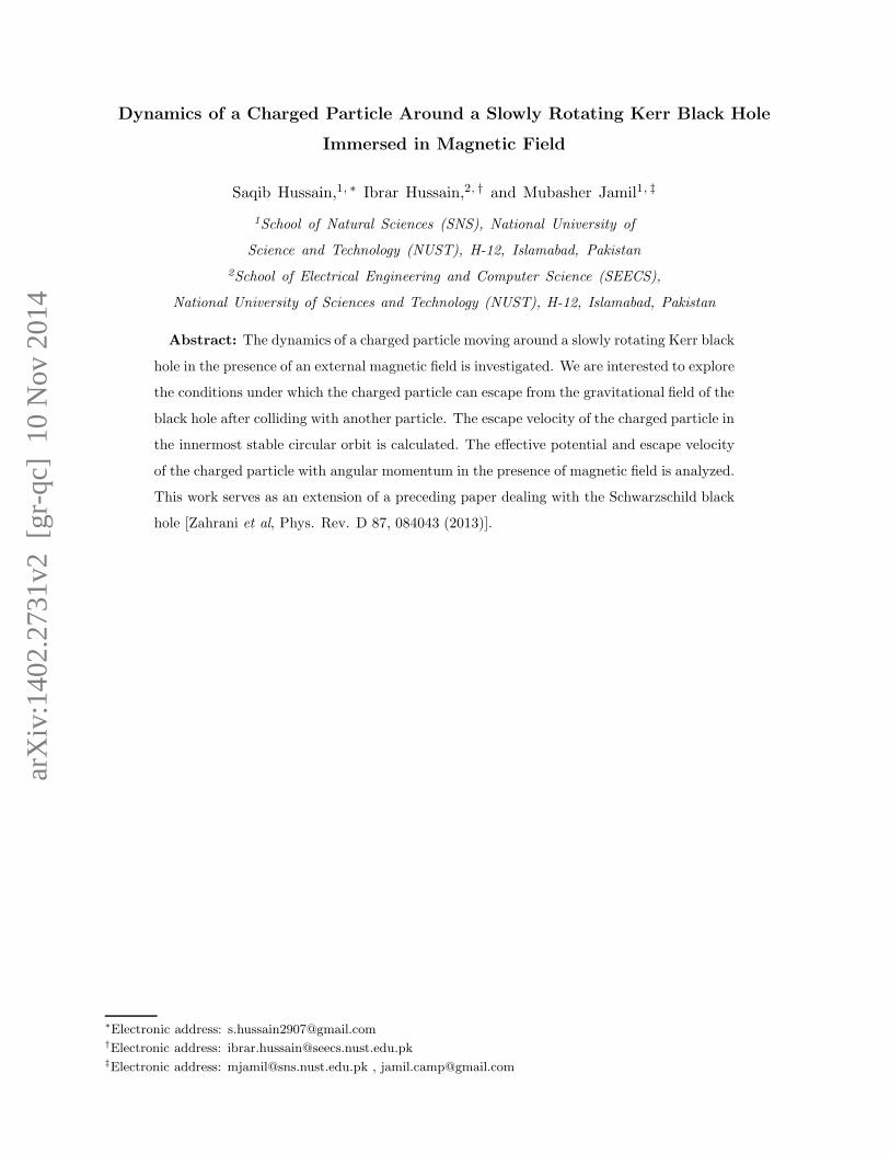
We solved the equation (36) numerically by using the built in command NDSolve of Mathematica.
As ISCO exists at r = 3rg, and using ρ = rrg
and σ = τrg, our initial conditions for solving (36)
become ρ(1) = 3 and ρ(1) = 3. We get the interpolating function ρ(σ) as the solution of the
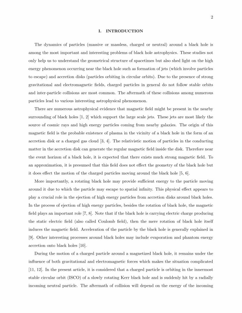
equation (36) which we plotted in figure 1 against σ. In figure 2 we have plotted the radial velocity
(derivative of the interpolating function) vs σ which shows that the particle will escape to infinity
according to the initial conditions.
As is the case of a neutral particle, we assume that the collision does not change the azimuthal
angular momentum of the particle but it changes the transverse velocity v > 0. Due to this, the
angular momentum and the energy of the particle will change as ℓ → ℓt and Eo → E respectively
which is given by
ℓ2t = ρ2v2⊥ + ρ4[
1
ρ2
(
aEo2(ρ− 1)
+ ℓ
)
− b
]2
, (37)
E =1
ρ6o(ρo − 1)
[
aρ3o(1− ρo)(ℓt − 2bρ2o(ρo − 1))
+
(
ρ6o(ρo − 1)2(a2(
ℓt − 2bρ2o(ρo − 1))2)
+ρ3o(ρo − 1)(
ρ2o + (ℓt + bρ2o)2)
)12]
. (38)
Here ℓt is the dimensionless form of L given by equation (13). For the unbound motion E ≥ 1. By
solving (38) and putting E = 1, we get escape velocity of the particle as given below
v⊥ = ± 1
4ρ2(ρ− 1)
[
4(ρ− 1)[√
a2ρ2 + ρ4(ρ− 1)− 2abρ4(ρ− 1)(2ρ − 1)
−aρ+ ρ(ρ− 1)(bρ2 + (ℓ− bρ2)2)]
+ aρEo[
4(ρ− 1)(ℓ− bρ2)]
]
(39)
We now discuss the behavior of the particle when it escapes to asymptotic infinity. For simplicity
we consider the particle initially in ISCO. The parameter ℓ and b are defined in term of ρo and
only E specifies the motion of the particle. We can express the parameters ℓ and b in term of ρo
by simultaneously solving the equations dEodρ
= 0, and d2Eodρ2
= 0, for ℓ and b. But the first derivative
and second derivative of effective potential are very complicated and we cannot find the explicit
expression for ℓ and b in term of ρ.

11
V. TRAJECTORIES FOR ESCAPE ENERGY
Here we investigate the dynamics of particle for the positive energy E+. Particles with negative
energy exist only inside the static limit surface (rst = 2m) orbiting in the retrograde orbits and do
not have the chance to escape. The equation for the rotational (angular) variable φ is
dφ
dσ=
ℓ
ρ2− b+
aEρ3(1− ρ)
. (40)
The Lorentz force acting on the massive charged particle is attractive when dφ/dσ < 0 and vice
versa. All the figures (3-8) correspond to Eq. (35). In figure-3, the shaded region corresponds
to unbound motion while the unshaded region refers to bounded trajectories of the particle. The
curved line represents the minimum energy required for the particle to escape form the vicinity of
the black hole. It can be seen from figure-4 that for large values of angular momentum, the plot is
similar to the effective potential of Schwarzschild black hole [16]. In figure 4, Emax corresponds to
unstable circular orbit and Emin refers to ISCO.
The effective potential E of a particle moving in a slowly rotating Kerr spacetime is plotted as
a function of radial coordinate ρ for different values of angular momentum ℓ in figure 5. We can
see from figure 5 that for large value of angular momentum, the maxima is shifting upward. For a
particle to be captured by the black hole it is required that the energy which should be greater then
this maxima. If its energy is less than this maxima there are two possibilities for a particle either
it will escape to infinity or it might start moving in ISCO. If energy of the particle E < 1 then it
will stay in some stable orbit and if E > 1 then it will escape to infinity. In figure 5 we plotted
effective potential against ρ for different value of angular momentum. For ℓ > 0 the Lorentz force
is repulsive. Hence it can be concluded from figure 5 that the possibility of a particle to escape
after collision from the vicinity of the black hole is greater for larger value of ℓ+ as compare to the
lesser value of it. For ℓ < 0 the lorentz force is attractive. Therefore, the possibility of a particle to
escape after collision is less for larger value of ℓ− as compared to smaller value of ℓ−, represented
in figure 6. The graph for ℓ = 0 and b = 0 in figure 6 corresponds to photon as there is no stable
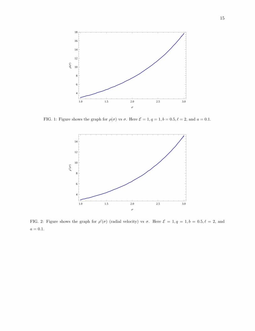
region. Moreover, we compare the effective potential for ℓ = 10 and ℓ = −10 in figure 7. It can
be seen that the stability is larger for ℓ = −10. Therefore it is concluded that for the attractive
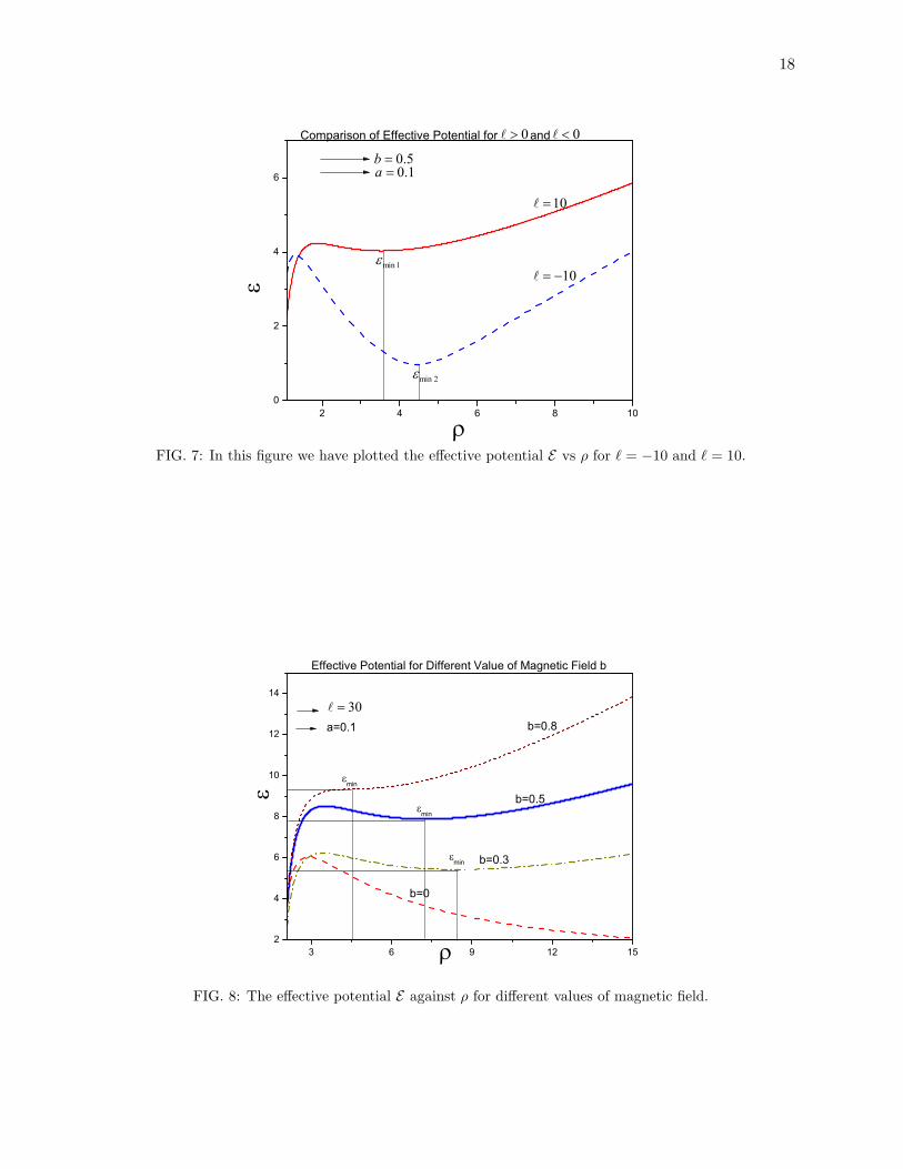
Lorentz force (ℓ = −10), particle required more energy to escape. It can be seen from figure 8 that
with the increase in the strength of magnetic field, the local minima of the effective potential is
shifting toward the horizon. This local minima corresponds to ISCO, which is in agreement with
the result of [15].

12
VI. TRAJECTORIES FOR ESCAPE VELOCITY
For all the figures of escape velocity we have denoted v⊥ ≡ vesc. From Eq. (38) we calculate the
escape velocity by substituting E = 1. Figures 9-12 correspond to Eq. (39). In figure 9, the shaded
region corresponds to escape velocity of the particle and the solid curve represents the minimum
velocity required to escape from the vicinity of the black hole to infinity. The unshaded region
represents the bound motion around the black hole. In figure 10 the shaded region corresponds
to escape velocity of the particle and the solid curve represents the minimum velocity required
to escape from the vicinity of the black hole. The unshaded region represents the bound motion
around the black hole.
In figure 11 we plotted escape velocity of a particle moving in ISCO as a function of radial
coordinate ρ for different values of magnetic field b. It can be seen from figure 11 that due to the
presence of magnetic field in the vicinity of black hole escape velocity of the particle increases.
Therefore we can say that in the presence of magnetic field b, the possibilities of the particle to
escape is greater then the case when magnetic field is absent i.e. b = 0. We plotted the escape
velocity against ρ in figure 12 for different values of angular momentum ℓ. We can see from the
figure 12 that the the escape velocity is increasing for large value of ℓ. Hence we can conclude that
if particle has larger value of angular momentum ℓ then it can easily escape to infinity as compared
to the particle with smaller value of angular momentum ℓ regardless of the magnetic field.
VII. DISCUSSION
We have studied the dynamics of a neutral and a charged particle around the slowly rotating
Kerr black hole which is immersed in a magnetic field. Therefore the particle is under the influence
of both gravitational and electromagnetic forces. We have obtained equations of motion by using
Lagrangian formalism. We have derived the expression for magnetic field present in the vicinity of
slowly rotating Kerr black hole. We have calculated the minimum energy for a particle to escape
from ISCO to infinity. With zero spin i.e. a = 0, our results reduce to the case of the Schwarzschild
black hole [12].
The behavior of effective potential and escape velocity against magnetic field and angular mo-
mentum are discussed in detail. It is shown in figures 4, 9 and 10 under what conditions particle
can escape from the vicinity of the black hole to spatial infinity. For larger values of the angular
momentum, behavior of the effective potential is similar to that of the Schwarzschild black hole

13
[12]. It is concluded that magnetic field largely effects the motion of the particle in the vicinity of
the black hole. This effect decreases far away from the black hole. It is found that as the value
of magnetic field parameter is increased, the local minima of effective potential shifted towards
the horizon, as shown in figure 8. This indicates that the ISCO shrinks as strength of magnetic
field increases. It is concluded from the figures 5 and 12 that if particle has large value angular
momentum ℓ+ then it can escape easily as compare to particle with smaller angular momentum
ℓ+. Figure 7 shows that for attractive Lorentz force (ℓ−) the stability is larger in comparison with
repulsive Lorentz force (ℓ+).
Escape velocity vesc, for different values of magnetic field b is plotted in figure 11. It is found
that due to the presence of magnetic field in the vicinity of black hole escape velocity of the particle
increases. Therefore we found that the possibility of the particle to escape from the vicinity of
black hole to infinity is greater in the presence of magnetic field as compared to the case when
magnetic field is absent b = 0.
Acknowledgment
M. Jamil and S. Hussain would like to thank the Higher Education Commission, Islamabad,
Pakistan for providing financial support under project grant no. 20-2166.
[1] C. V. Borm, M. Spaans, Astron, Astrophy, 553, L9 (2013).
[2] V. Frolov, The Galactic Black Hole (Editors: H. Falcke, F.H. Hehl), IoP 2003.
[3] J. C. Mckinney, R. Narayan, Mon. Not. Roy. Astron. Soc. 375, 523 (2007).
[4] P. B. Dobbie, Z. Kuncic, G. V. Bicknell, R. Salmeron, Proceedings of IAU Symposium 259 Cosmic
Magnetic Field: From Planets, To Stars and Galaxies(Tenerife, 2008).
[5] R. Znajek, Nature 262, 270 (1976).
[6] R. D. Blandford, R. L. Znajek, Mon. Not. Roy. Astron. Soc. 179, 433 (1977).
[7] S. Koide, K. Shibata, T. Kudoh, D. l. Meier, Science 295, 1688(2002).
[8] S. Kide, Phys. Rev. D 67, 104010 (2003).
[9] O. B. Zaslavskii, Class. Quant. Grav. 28, 105010 (2011).
[10] M. Jamil, A. Qadir, Gen. Rel. Grav. 43, 1069 (2011); B. Nayak, M. Jamil, Phys. Lett. B 709, 118
(2012); M. Jamil, D. Momeni, K. Bamba, R. Myrzakulov, Int. J. Mod. Phys D 21, 1250065 (2012); M.
Jamil, M. Akbar, Gen. Rel. Grav. 43, 1061 (2011).
[11] D. V. Gal’tsov, V. I. Petukhov, Sov. Phys. JEPT 47(3), 419 (1978).
[12] A. M. A. Zahrani, V. P. Frolov, A, A. Shoom, Phys. Rev. D 87, 084043 (2013).

14
[13] M. Baados, J. Silk, and S. M. West, Phys. Rev. Lett. 103, 111102 (2009).
[14] S. Hod, Phys. Rev. D 87, 024036 (2013) ; C. Chakraborty, Eur. Phys. J. C74, 2759 (2014); C. Bambi,
E. Barausse, Phys. Rev. D 84, 084034 (2011) ; B. Toshmatov, A. Abdujabbarov, B. Ahmedov, Z.
Stuchlk, arXiv:1407.3697 ; T. Harada, M. Kimura, Phys. Rev. D 83, 024002 (2011) ; P. Pradhan,
arXiv:1407.0877
[15] A. N. Aliev, N. O. Ozdemir, Mon. Not. Roy. Astron. Soc. 336, 241 (1978).
[16] V. P. Frolov, A. A. Shoom, Phys. Rev. D 82, 084034 (2010).
[17] V. P. Frolov, Phys. Rev. D 85, 024020 (2012).
[18] J. Buchner, and L. M. Zelenyi, J. Geophys. Res. 94, 821 (1989).
[19] J. Buchner, and L. M. Zelenyi, J. Geophys. Res. Lett. 17, 127 (1990).
[20] D. Raine, and E. Thomas, Black Holes An Introduction (Imperial College Press, 2005).
[21] B. Punsly, Black Hole Gravitohydrodynamics (Springer-Verlag, Berlin, 2001).
[22] I. Hussain, Mod. Phy. Lett. A 27, 1250068 (2012).
[23] S. Chandrasekher, The Mathematical Theory of Black Holes (Oxford University Press, 1983).
[24] F. De Paolis, A. Geralico, G. Ingrosso, A.A. Nucita, A. Qadir, Astron. Astrophys. 415,1 (2004).
[25] J. Sadeghi, B.Pourhassan, Eur. Phys. J. C 72, 1984 (2012).
[26] T. Harko, Z. Kovcs, F. S.N. Lobo, Class. Quant. Grav. 28, 165001 (2011); ibid, Class. Quant. Grav.
26, 215006 (2009).
[27] S. Chakrabarti, The Sun, The Stars, The Universe and General Relativity edited by R. Ruffini and G.
Vereshchagin (AIP 2010).
[28] A. Qadir, A.A. Siddiqui, Int. J. Mod. Phys. D 16, 25 (2007).
[29] M. P. Hobson, G. P. Efstathiou, A. N. Lasenby, General Relativity An Introdction for Physicists
(Cambridge University Press 2006).
15
1.0 1.5 2.0 2.5 3.0
4
6
8
10
12
14
16
18
Σ
ΡHΣL
FIG. 1: Figure shows the graph for ρ(σ) vs σ. Here E = 1, q = 1, b = 0.5, ℓ = 2, and a = 0.1.
1.0 1.5 2.0 2.5 3.0
4
6
8
10
12
14
Σ
Ρ¢HΣL
FIG. 2: Figure shows the graph for ρ′(σ) (radial velocity) vs σ. Here E = 1, q = 1, b = 0.5, ℓ = 2, and
a = 0.1.

16
1.0 1.5 2.0 2.5 3.0
0.4
0.6
0.8
1.0
1.2
1.4
1.6
1.8
Ρ
Ε
FIG. 3: In this figure we plot Effective potential E as a function of ρ for ℓ = 5, b = 0.5 and a = 0.1.
0.0 0.5 1.0 1.5 2.0 2.5 3.0 3.50.0
0.5
1.0
1.5
2.0
2.5
3.0
2max
2min
Veff
FIG. 4: Here we plot the effective potential against ρ for ℓ = 20, b = 0.5, and a = 0.1. In this figure Emax
corresponds to unstable circular orbit and Emin corresponds to stable circular orbit.

17
3.5 7.0 10.5 14.0
1
2
3
4
4
7
10
min
0b1.0a
Effective Potential in the Absence of Magnetic Field
20
FIG. 5: The effective potential E is plotted as a function of radial coordinate ρ for different values of angular
momentum ℓ.
2 4 6 8 100
2
4
1min2min
1.0a
5
2 0,0 b
10
Efective Potential for Negative Values of Angular Mometum
5.0b
FIG. 6: The effective potential E is plotted against radial coordinate ρ for different values of negative angular
momentum ℓ.
18
2 4 6 8 100
2
4
6 1.0a
1min
00
10
10
Comparison of Effective Potential for and
2min
5.0b
FIG. 7: In this figure we have plotted the effective potential E vs ρ for ℓ = −10 and ℓ = 10.
3 6 9 12 152
4
6
8
10
12
14
min
min
b=0.5
b=0
b=0.3
b=0.8
min
a=0.1
Effective Potential for Different Value of Magnetic Field b
30
FIG. 8: The effective potential E against ρ for different values of magnetic field.

19
1.5 2.0 2.5 3.0 3.5 4.0
4.0
4.5
5.0
Ρ
v
FIG. 9: Here we have plotted the escape velocity against ρ for ℓ = 5, b = 0.5 and a = 0.1.
1.5 2.0 2.5 3.0
-5.0
-4.5
-4.0
Ρ
v
FIG. 10: In this figure we have plotted the escape velocity against ρ for ℓ = 5, b = 0.5 and a = 0.1.
2.0 2.5 3.0 3.5 4.00
2
4
6
8
10
12
14
1o
1.0a
0b
5.0b
v esc
8.0b5
Esacpe Veloity for Different Values of Magnetic Field
FIG. 11: Escape velocity vesc against ρ for different values of magnetic field b.

20
1.4 1.6 1.8 2.0 2.2 2.4 2.6 2.8
0
5
10
15
20
25
1o
1.0a
3
v esc 5
5.0b
Escape Velocity for Different Values Angular Momentum
FIG. 12: Escape velocity vesc against ρ for different values of angular momentum ℓ.

3 4 5 6 7 8 9 10
0.5
0.6
0.7
0.8
0.9
r
B