PROBLEMS RELATED TO I NVARIANT THEORY OF TORUS

AND FINITE GROUPS

By

Santosha Kumar Pattanayak

Thesis Supervisor : Professor S. Senthamarai Kannan

P1(C)= Flag variety of SL2(C)

A Thesis in Mathematics submitted to the

Chennai Mathematical Institute

in partial fulfillment of the requirements

for the degree of Doctor of Philosophy

March 2011

Chennai Mathematical InstitutePlot No-H1, SIPCOT IT Park,

Padur Post, Siruseri,Tamilnadu-603103

CHENNAIMATHEMATICALINSTITUTE Santosha Kumar Pattanayak

Plot No.H1, SIPCOT IT Park

Padur Post, Siruseri-603 103

Tamil Nadu, India

Phone: +91 - 44 - 2747 0226

E-mail: santosh@cmi.ac.in

DECLARATION

I declare that the thesis entitled“Problems related to Invariant theory of torus and finitegroups” submitted by me for the Degree of Doctor of Philosophy in Mathematics is the recordof academic work carried out by me during the period from October 2005 to March 2011 underthe guidance of Professor S. Senthamarai Kannan and this work has not formed the basis forthe award of any degree, diploma, associateship, fellowship or other titles in this University orany other University or Institution of Higher Learning.

Santosha Kumar Pattanayak

ii

CHENNAIMATHEMATICALINSTITUTE Professor S. Senthamarai Kannan

Plot No.H1, SIPCOT IT Park

Padur Post, Siruseri-603 103

Tamil Nadu, India

Phone: +91 - 44 - 2747 0226

E-mail: kannan@cmi.ac.in

Certificate

I certify that the thesis entitled“Problems related to Invariant theory of torus and finitegroups” submitted for the degree of Doctor of Philosophy in Mathematics by Santosha KumarPattanayak is the record of research work carried out by him during the period from October2005 to March 2011 under my guidance and supervision, and that this work has not formed thebasis for the award of any degree, diploma, associateship, fellowship or other titles in this Uni-versity or any other University or Institution of Higher Learning. I further certify that the newresults presented in this thesis represent his independentwork in a very substantial measure.

Chennai Mathematical InstituteDate: March, 2011

Professor S. Senthamarai KannanThesis Supervisor

iv

Acknowledgement

First of all I would like to express my gratefulness to my advisor Professor S. SenthamaraiKannan for introducing me to the research area of Invariant theory. I am specially grateful tohim for introducing me to the problem in a beautiful way at thetime when I was an absolutenovice; for his efforts to understand my mindset and therebyadvising me appropriately; for hispatience in dealing with me; for his continuous encouragement. I deeply appreciate his way ofworking, start from basics, and must say that it has had a great influence on me. I owe muchmore to him than I can write here.

I had the opportunity to talk Mathematics with several people. I am especially grateful toPranab Sardar, Dr. P. Vanchinathan and Professor K. N. Raghavan who were always welcom-ing, happy to talk about mathematics and answer my questions. I am grateful to Professor V.Balaji and Dr. Clare D’Cruz for their encouragement and constant help. I have had very helpfulmathematical discussions with Professor R. Sridharan, Dr.Suresh Nayak and Rohith Varma. Iam grateful to all of them.

I am really grateful to Dr. Peter O’Sullivan for carefully reading all my papers in arxiv andfor giving me many valuable remarks which helped me to improve my thesis tremendously.I would like to thank Professor Pramathanath Sastry and Dr. M. Sundari for many valuablecomments on my thesis-synopsis.

I take this opportunity to thank many of my colleagues, especially Abhishek and Prakashfor helping me to write the C-program given in appendix-A. I would like to thank MahenderSingh with whom I have shared many good times and for helping me in many ways to improvethis thesis.

I would like to thank NBHM (National Board for Higher Mathematics) and the ChennaiMathematical Institute for supporting me financially throughout the Ph.D program. In partic-ular, I would like to thank the Chennai Mathematical Institute for providing me with variousfacilities and an environment to do independent work.

I would like to thank the office staff of the Chennai Mathematical Institute (CMI) for theiralltime ready-to-help attitude in any kind of official matter. I would also like to thank all theacademic staff at the Chennai Mathematical Institute who have been very friendly to me.

Finally this endeavor would not have existed without support from my parents. There cannot be any substitute for the unconditional support and loveof my parents, who have given mecomplete freedom over the years.

vi

Dedicated to my advisor

viii

Table of contents

0 Introduction 1

0.1 General Layout of the Thesis . . . . . . . . . . . . . . . . . . . . . . . .. . . 2

1 Algebraic Groups 3

1.1 Basic Definitions and Properties . . . . . . . . . . . . . . . . . . . .. . . . . 3

1.1.1 Definition and Examples . . . . . . . . . . . . . . . . . . . . . . . . . 3

1.1.2 Actions and Representations of Algebraic Groups . . . .. . . . . . . . 5

1.2 Jordan Decomposition in Linear Algebraic Groups . . . . . .. . . . . . . . . 6

1.3 Lie Algebra of an Algebraic Group . . . . . . . . . . . . . . . . . . . .. . . . 7

1.4 Homogeneous Spaces . . . . . . . . . . . . . . . . . . . . . . . . . . . . . . 8

1.5 Tori . . . . . . . . . . . . . . . . . . . . . . . . . . . . . . . . . . . . . . . . 10

1.6 Solvable Groups and Borel Subgroups . . . . . . . . . . . . . . . . .. . . . . 11

1.7 Root Systems and Semi-simple Theory . . . . . . . . . . . . . . . . .. . . . . 13

1.7.1 Classification of Root Systems . . . . . . . . . . . . . . . . . . . .. . 14

1.7.2 Classification of Semi-simple Lie Algebras and Algebraic Groups . . . 16

1.7.3 Weights and Representations . . . . . . . . . . . . . . . . . . . . .. . 18

1.8 Reductive Group . . . . . . . . . . . . . . . . . . . . . . . . . . . . . . . . . 21

1.8.1 Classification of Reductive Algebraic Groups . . . . . . .. . . . . . . 23

1.9 Parabolic Subgroups . . . . . . . . . . . . . . . . . . . . . . . . . . . . . .. 23

1.9.1 The Weyl Group of a Parabolic Subgroup . . . . . . . . . . . . . .. . 24

x

1.10 Schubert Varieties . . . . . . . . . . . . . . . . . . . . . . . . . . . . . .. . . 24

1.10.1 Line Bundles on G/P . . . . . . . . . . . . . . . . . . . . . . . . . . . 25

1.10.2 Weyl Module . . . . . . . . . . . . . . . . . . . . . . . . . . . . . . . 27

2 Invariant theory 28

2.1 Introduction . . . . . . . . . . . . . . . . . . . . . . . . . . . . . . . . . . . .28

2.2 Finite Generation . . . . . . . . . . . . . . . . . . . . . . . . . . . . . . . .. 29

2.3 Construction of Invariants . . . . . . . . . . . . . . . . . . . . . . . .. . . . . 30

2.4 Hilbert Series of an Invariant Algebra . . . . . . . . . . . . . . .. . . . . . . 31

2.5 UFD and Polynomial Algebra . . . . . . . . . . . . . . . . . . . . . . . . .. 32

2.6 Cohen-Macaulay Property . . . . . . . . . . . . . . . . . . . . . . . . . .. . 35

2.7 Depth of an Invariant Ring . . . . . . . . . . . . . . . . . . . . . . . . . .. . 37

2.8 Noether’s Degree Bound . . . . . . . . . . . . . . . . . . . . . . . . . . . .. 38

2.9 Vector Invariants . . . . . . . . . . . . . . . . . . . . . . . . . . . . . . . .. 41

2.10 Geometric Invariant Theory . . . . . . . . . . . . . . . . . . . . . . .. . . . . 44

2.10.1 Group Actions on Algebraic Varieties . . . . . . . . . . . . .. . . . . 44

2.10.2 G.I.T. Quotients . . . . . . . . . . . . . . . . . . . . . . . . . . . . . .47

2.10.3 Linearization of the Action . . . . . . . . . . . . . . . . . . . . .. . . 50

3 Torus Quotients of Homogeneous Spaces 51

3.1 Introduction . . . . . . . . . . . . . . . . . . . . . . . . . . . . . . . . . . . .51

3.2 Preliminary Notations and Combinatorial Lemmas . . . . . .. . . . . . . . . 52

3.3 Minimal Schubert Varieties inG/P admitting Semi-stable Points . . . . . . . . 57

3.3.1 Classical Types . . . . . . . . . . . . . . . . . . . . . . . . . . . . . . 57

3.3.2 Exceptional Types . . . . . . . . . . . . . . . . . . . . . . . . . . . . 64

3.4 Coxeter Elements admitting Semi-stable Points . . . . . . .. . . . . . . . . . 69

xi

4 Projective Normality of GIT Quotient Varieties 80

4.1 Introduction . . . . . . . . . . . . . . . . . . . . . . . . . . . . . . . . . . . .80

4.2 Solvable Case . . . . . . . . . . . . . . . . . . . . . . . . . . . . . . . . . . . 81

4.3 Group Generated by Pseudo Reflections . . . . . . . . . . . . . . . .. . . . . 83

4.4 Vector Invariants and Projective Normality . . . . . . . . . .. . . . . . . . . . 84

4.5 Normality, Projective Normality and EGZ Theorem . . . . . .. . . . . . . . . 89

4.5.1 Normality of a Semigroup . . . . . . . . . . . . . . . . . . . . . . . . 89

4.5.2 A Result connecting a Normal Semigroup and the EGZ Theorem . . . 90

4.6 A Counter Example . . . . . . . . . . . . . . . . . . . . . . . . . . . . . . . . 92

Appendix-A 93

Appendix-B 98

Bibliography 109

xii

Chapter 0

Introduction

One of the classical problems in invariant theory is the study of binary quantics. The mainobject is to give an explicit description of the ringK[V ]SL2, whereV is the space of all homo-geneous forms of degreen in two variables and study the geometric properties ofSL2 quotientsof projective space for a suitable choice of linearization.The natural generalization of this clas-sical problem is the following;

Let K be an algebraically closed field. LetG be a semi-simple algebraic group overK,T a maximal torus ofG, B a Borel subgroup ofG containingT , N the normalizer ofT inG and,W = N/T the Weyl group. For a parabolic subgroupQ of G containingB, considerthe quotient varietyN\\(G/Q). In the case whenG = SLn(K), the special linear group andQ is the maximal parabolic subgroup ofSLn(K) associated to the simple rootα2, one knowsthatG/Q is the GrassmannianG2,n of two- dimensional subspaces of ann dimensional vectorspace. One also has an isomorphism:

N\\(G/Q)ss(L2) = N\\(G2,n)ss(L2) ≃ SL2\\(P(V ))ss,

whereV is the vector space of homogeneous polynomials of degreen in two variables andL2

is the line bundle associated to the fundamental weight2, and the varietySL2\\P(V )ss isprecisely the space of binary quantics, (for example, see the proof of Theorem-1 and the proofof Theorem-4 of [100]). More generally one has the followingisomorphism;

T\\(G/P )ss(Lr) = T\\(Gr,n)ss(Lr) ≃ SLr\\(P

r−1)n,

whereG = SLn(K), P is the maximal parabolic subgroup associated to the simple root αr,Gr,n is the Grassmannian ofr-dimensional subspaces of ann dimensional vector space andLr

is the line bundle onG/P = Gr,n associated to r.

One direction of our work is the study of projective normality of GIT quotient varieties forfinite group actions and another direction is to study the semi-stable points for a maximal torusaction on the homogeneous spaceG/P , whereG is a semi-simple simply connected algebraicgroup andP is a parabolic subgroup ofG. Both studies arose out of an attempt to understandthe quotientSn\(T\\G2,n)

ss.

1

0.1 General Layout of the Thesis

We now describe the organization of this thesis. The thesis consists of four chapters. A con-scious effort is made to make this thesis self-contained andreader-friendly. Chapters 1 and2 are preliminary in nature and are intended to introduce most of the basic concepts used inthis thesis. We do not aim to give a complete account of these topics but try to give most ofthe definitions and results used later and provide appropriate references for these results. Thenwhile using these results we refer to the first two chapters instead of referring to the originalpapers, which we have anyway referred to in the introductorychapters. Chapters 3 and 4 reportthe work done by the author.

In Chapter 1 we give a brief account of the theory of algebraicgroups. In this chapter, weintroduce some definitions and terminologies which we keep using throughout this thesis. Fora detailed study of the theory of algebraic groups, we refer the reader to [2], [46], [115].

Chapter 2 is a survey of computational invariant theory of finite groups as well as reduc-tive algebraic groups. In this chapter we present many classical as well as modern results ininvariant theory. In the last section of this chapter “Geometric invariant theory” is introduced.

Chapter 3 is about torus action onG/P . Mainly under the action of a maximal torus wedescribe all the minimal-dimensional Schubert varieties in G/P admitting semi-stable pointswith respect to an ample line bundle, whereG is a semi-simple simply connected algebraicgroup andP is a maximal parabolic subgroup ofG. In this chapter we also describe all Coxeterelementsw ∈ W for which the corresponding Schubert varietyX(w) admits a semi-stablepoint for the action of a maximal torus with respect to a non-trivial line bundle onG/B.

In Chapter 4 we investigate the projective normality of GIT quotient varieties for the actionof finite groups. At the end of this chapter, we also take the opportunity to describe some of thequestions that remain to be answered.

At the end of this thesis we have included two appendices, named as Appendix-A andAppendix-B. In Appendix-A we give a C-program that is used inChapter 3. Appendix-Bcollects the most important pieces of information about theLie algebras associated to semi-simple algebraic groups.

2

Chapter 1

Algebraic Groups

This chapter is the most basic and at the same time the most essential part of this thesis. Herewe define all the required terms and review the basic results (without proof) that are neededlater in this thesis. The theory of linear algebraic groups is a well-developed topic and there aremany excellent books available on it. Mostly, we refer to [2,46, 115] for simplicity.

1.1 Basic Definitions and Properties

1.1.1 Definition and Examples

An affine algebraic group is a groupG equipped with a structure of an affine variety such thatthe multiplication mapµ : G × G → G, µ(g1, g2) = g1g2 and the inverse mapi : G →G, i(g) = g−1 are morphisms of affine varieties.

Since any variety has atleast one smooth point and the actionof G on itself by left translationis transitive,G is a smooth variety.

A homomorphism of algebraic groupsφ : G1 → G2 is a homomorphism of groups and alsoa morphism of varieties. An isomorphism of algebraic groupsis a bijective homomorphismφ : G1 → G2 such thatφ−1 is also a morphism of varieties. An isomorphism fromG to itselfis called an automorphism.

Example : An example of an affine algebraic group is the groupGLn of n × n invertiblematrices. Indeed, we have

GLn = {

(X 00 xn+1

)

: det(X)xn+1 = 1}

and forX, Y ∈ GLn, the entries of the productXY are polynomial functions in the entries ofX andY . We callGLn, the general linear group.

3

Remark: In this chapter we consider only affine algebraic groups, so the adjective ”affine” willbe sometimes omitted.

A closed subgroup ofGLn is called a linear algebraic group. It is easy to see that ifH isa subgroup of an algebraic groupG and also a closed subvariety ofG, thenH is an algebraicsubgroup. So we have several examples of algebraic subgroups ofGLn. We list some of thembelow:

Example: Dn: the group of invertible diagonal matrices.Bn: the group of upper triangular matrices.Un: the group of unipotent upper triangular matrices.SLn = {X ∈ GLn : det(X) = 1}: the special linear group.On = {X ∈ GLn : X tX = In}: the orthogonal group, (whereX t denotes the transpose of thematrixX andIn is the identity matrix inGLn).SOn = SLn∩On: the special orthogonal group. This group can also be definedas{X ∈ GLn :

X tJX = J}, whereJ ∈ GLn is the matrix

(0 In

2

In2

0

)

if n is even and

1 0 00 0 In−1

2

0 In−1

2

0

if n is odd (charK 6= 2).Sp2n = {X ∈ GL2n : X tJX = J}: the symplectic group, whereJ ∈ GL2n is the matrix(

0 In

−In 0

)

.

Example : (Finite groups). Any finite setX with n elements admits a canonical structure ofan affine algebraic variety (overK). This variety hasn irreducible one-point components andthe algebra of regular functionsK[X] is the direct sum ofn copies of the fieldK: K[X] =K ⊕ · · · ⊕ K. In particular, anyK-valued function onX is regular, and any mapX → Yto another affine varietyY is a morphism. This shows that any finite groupG has a canonicalstructure of an affine algebraic group.

Example : (Additive and multiplicative groups). The additive groupGa is the affine lineK1 with group lawµ(x, y) = x + y and i(x) = −x. The multiplicative groupGm is theaffine open subsetK× ⊂ K with µ(x, y) = xy, i(x) = x−1. Clearly, they are commutativeone-dimensional algebraic groups. The groupGm may be realized asGL1, but for a matrixrealization ofGa one needs2 × 2-matrices:

{

(1 c0 1

)

: c ∈ K}.

InfactGa andGm are the only connected one-dimensional algebraic groups.

Again, the direct product of two affine algebraic groups has acanonical structure of anaffine algebraic group. So, we can construct many examples ofalgebraic groups, for example:the direct productT = Gk

m is a commutative algebraic group called an algebraic torus.

For an algebraic groupG the connected componentG0 containing the identity element is aclosed normal subgroup of finite index and coincide with the irreducible component contain-ing identity. So, the notions of irreducibility and connectedness coincide for affine algebraic

4

groups. SinceGLn is an open subset ofMn×n, it is irreducible. So,GLn is connected. One cancheck that the commutator subgroup[G, G] of a connected algebraic groupG is connected. Inparticular,SLn is connected being commutator ofGLn.

1.1.2 Actions and Representations of Algebraic Groups

Let X be an algebraic variety andG an algebraic group. A morphismG × X → X is said tobe an algebraic action, if it satisfies the following properties:

(i) e.x = x for anyx ∈ X;

(ii)g1.(g2.x) = (g1g2).x for anyg1, g2 ∈ G, x ∈ X.

Example: There are three actions of a groupG on itself, which are considered most often.Namely,g.g1 = gg1, g.g1 = g1g

−1, g.g1 = gg1g−1.

We refer to [46] for the definition of orbit, stabilizer and the set of fixed points of an action.The subsetXG of G-fixed points is closed inX and for anyx ∈ X the stabilizerGx is a closedsubgroup ofG. Further, the orbitG.x is a smooth locally closed subvariety ofX and orbit ofthe smallest dimension is closed inX. Moreover,dim(G) = dim(Gx) + dim(G.x).

Definition : A rational representation of an algebraic groupG in a finite dimensional vectorspaceV is a homomorphismρ : G → GL(V ) of algebraic groups. HereV is said to be arationalG-module.

Any representationρ : G → GL(V ) defines an actionG × V → V, g.v = ρ(g)v. Suchactions are called linear.

Remark : A rational representation ofGLn is a homomorphismρ : GLn → GL(V ) such thatthe matrix entries ofρ(A) are polynomials inaij ,

1det(A)

, whereV is a finite dimensional vector

space. The presence of1det(A)

motivates the term ”rational”.

Remark : Standard constructions of representation theory (restrictions to invariant subspaces,quotient and dual representations, direct sums, tensor products, symmetric and exterior powersetc.) allow to produce numerous rationalG-modules from given ones.

Remark : Any rational representationρ : G → GL(V ) defines a natural algebraic action onthe projective spaceP (V ); g.[v] := [ρ(g)v].

If X is an affineG-variety then, there is a natural action ofG on the algebra of regularfunctionsK[X]:

(g.f)(x) := f(g−1.x); f ∈ K[X], x ∈ X, g ∈ G.

The G-moduleK[X] is locally finite i.e. any elementf ∈ K[X] is contained in a finitedimensional rational submodule.

5

The next theorem explains why we call an affine algebraic group linear.

Theorem 1.1.1.Any affine algebraic group is isomorphic to a closed subgroupof GLn forsomen ∈ N.

1.2 Jordan Decomposition in Linear Algebraic Groups

In this section we will assume thatK is an algebraic closed field.A matrix x ∈ Mn(K) is semi-simple ifx is diagonalizable: there is ag ∈ GLn(K) such thatgxg−1 is a diagonal matrix. Also,x is unipotent ifx − In is nilpotent:(x − In)k = 0 for somenatural numberk. For givenx ∈ GLn(K), there exist elementsxs andxu in GLn(K) suchthatxs is semi-simple,xu is unipotent, andx = xs.xu = xu.xs. Furthermore,xs andxu areuniquely determined (see [46, pg. 96]). Now suppose thatG is an affine algebraic group. Wecan choosen and an injective homomorphismφ : G → GLn(K) of algebraic groups. Ifg ∈ G,the semi-simple and unipotent partsφ(g)s andφ(g)u of φ(g) lie in φ(G).The elementsgs andgu such thatφ(gs) = φ(g)s andφ(gu) = φ(g)u depend only ong and not on the choice ofφ (orn). The elementsgs andgu are called the semi-simple and unipotent part ofg, respectively. Anelementg ∈ G is semi-simple ifg = gs, and unipotent ifg = gu.

Theorem 1.2.1.(Jordan-Chevalley Decomposition ([46, pg. 99]). Ifg ∈ G, there exist uniqueelementsgs andgu in G such thatg = gs.gu = gu.gs, gs is semi-simple, andgu is unipotent.Further, Jordan decompositions are preserved by homomorphisms of algebraic groups.

For any algebraic groupG the setGu = {gu : g ∈ G} is a closed subset ofG. An algebraicgroupG is called unipotent if all of its elements are unipotent. ForexampleGa is unipotent.

A solvable (resp. nilpotent) algebraic group is an algebraic group which is solvable (resp.nilpotent) as an abstract group. Now letG be an arbitrary connected algebraic group. Supposethat A andB are two closed connected normal solvable subgroups ofG. ThenAB is againa closed connected normal solvable subgroup ofG containing bothA andB. It follows thatG contains a unique closed connected normal solvable subgroup of maximal dimension. Thisis called the radical ofG, denoted byR(G). An algebraic group is calledsemi-simpleif itsradicalR(G) = e. Similarly the unipotent radical ofG, denoted byRu(G) is the unique closedconnected normal unipotent subgroup of maximal dimension.An algebraic group is calledreductiveif its unipotent radicalRu(G) = e. SinceRu(G) is unipotent, it is nilpotent, hencesolvable. ThusRu(G) ⊆ R(G). So semi-simple groups are reductive.

For example,SLn is a semi-simple group butGLn has a one dimensional radical consistingof the scalar matrices. ThusGLn is not semi-simple, but since scalar matrices are semi-simple,its unipotent radical is trivial, soGLn is reductive.

6

1.3 Lie Algebra of an Algebraic Group

Let G be a linear algebraic group. The tangent bundleT (G) of G is the setHomK−alg(K[G],K[t]/(t2)) of K-algebra homomorphisms from the affine algebraK[G] of G to the algebraK[t]/(t2). If g ∈ G, the evaluation mapf 7→ f(g) from K[G] to K is aK-algebra isomor-phism. This results in a bijection betweenG andHomK−alg(K[G], K). Composing elementsof T (G) with the mapa + bt + (t2) 7→ a from K[t]/(t2) to K results in a map fromT (G) toG = HomK−alg(K[G], K). The tangent spaceT1(G) of G at the identity element1 of G is thefibre of T (G) over1. If X ∈ T1(G) andf ∈ K[G], thenX(f) = f(1) + tdX(f) + (t2) forsomedX(f) ∈ K. This defines a mapdX : K[G] → K which satisfies:

dX(f1f2) = dX(f1)f2(1) + f1(1)dX(f2), f1, f2 ∈ K[G]

Let µ∗ : K[G] → K[G] ⊗ K[G] be theK-algebra homomorphism which corresponds tothe multiplication mapµ : G×G → G. SetδX = (1⊗ dX) ◦µ∗. The mapδX : K[G] → K[G]is aK-linear map and a derivation:

δX(f1f2) = δX(f1)f2 + f1δX(f2), f1, f2 ∈ K[G].

Furthermore,δX is left-invariant:lgδX = δX lg for all g ∈ G, where(lgf)(g′) = f(g−1g′), f ∈K[G]. The mapX 7→ δX is aK-linear isomorphism ofT1(G) onto the vector space ofK-linearmaps fromK[G] to K[G] which are left-invariant derivations.

Let g = T1(G). Define[X, Y ] ∈ g by δ[X,Y ] = δX ◦ δY − δY ◦ δX . Theng is a vector spaceoverK and the map[·, ·] satisfies:

(1) [·, ·] is bilinear

(2) [X, X] = 0 for all X ∈ g

(3) [[X, Y ], Z] + [[Y, Z], X] + [[Z, X], Y ] = 0 for all X, Y, Z ∈ g (Jacobi identity).

Thereforeg is a Lie algebra overK. We call it the Lie algebra ofG.

Example : If G = GLn(K), theng is isomorphic to the Lie algebragln(K) which isMn(K)equipped with the Lie bracket[X, Y ] = XY − Y X,X, Y ∈ Mn(K).

Example : The Lie algebras of the algebraic groupsSLn, SOn, andSP2n aresln:= the trace

zero matrices,son:= the anti-symmetric matrices andsp2n := {

(A BC D

)

∈ GL2n : A =

−DT , B = BT , C = CT} respectively.

Let φ : G → G′ be a homomorphism of linear algebraic groups. Composition with thealgebra homomorphismφ∗ : K[G′] → K[G] results in a mapT (φ) : T (G) → T (G′). Thedifferentialdφ of φ is the restrictiondφ = T (φ)|g of T (φ) to g. It is aK-linear map fromg to

7

g′, and satisfiesdφ([X, Y ]) = [dφ(X), dφ(Y )], X, Y ∈ g.

That is,dφ is a homomorphism of Lie algebras. Ifφ is bijective, thenφ is an isomorphism ifand only ifdφ is an isomorphism of Lie algebras. IfK has characteristic zero, any bijectivehomomorphism of linear algebraic groups is an isomorphism.

In characteristic zero the correspondence between algebraic groups and their Lie algebrasis very nice. IfH is a closed subgroup of a connected linear algebraic groupG, then (via thedifferential of inclusion) the Lie algebrah of H is isomorphic to a Lie subalgebra ofg. Infactthe correspondenceH 7→ h is 1 − 1 and inclusion preserving between the collection of closedconnected subgroupsH of G and the collection of their Lie algebras, regarded as subalgebrasof g. And H is a normal subgroup ofG if and only if h is an ideal ing ([X, Y ] ∈ h wheneverX ∈ g andY ∈ h). If G is solvable (resp. nilpotent), theng is solvable (resp. nilpotent). IfG is semi-simple (resp. reductive), theng is semi-simple (resp. reductive). Recall that a Liealgebrag is said to be semi-simple ifrad(g): the maximal solvable ideal is 0 and reductive ifrad(g) = Z(g).

If g ∈ G, thenIntg : G → G, Intg(g0) = gg0g−1, g0 ∈ G, is an isomorphism of algebraic

groups. So,Ad(g) := d(Intg) : g → g is an isomorphism of Lie algebras and the mapAd : G → GL(g) is a homomorphism of algebraic groups, called theadjoint representationofG.

Jordan decomposition in the Lie algebra:We can define semi-simple and nilpotent elementsin g in a manner analogous to definitions of semi-simple and unipotent elements inG (asg isisomorphic to a Lie subalgebra ofgln(K) for somen). If X ∈ g, there exist unique elementsXs andXn ∈ g such thatX = Xs + Xn, [Xs, Xn] = [Xn, Xs] = 0, Xs is semi-simple, andXn is nilpotent.

1.4 Homogeneous Spaces

Let G be an affine algebraic group andH a closed subgroup ofG. The set of left cosetsG/Hadmits a natural transitiveG-action: g.g1H = gg1H. The following celebrated theorem ofChevalley gives a structure of an algebraic variety onG/H such that the action above becomesalgebraic.

Theorem 1.4.1.(Chevalley [14] (1951)). LetG be an affine algebraic group andH a closedsubgroup ofG. Then,

(1) There is a rational representationρ : G → GL(V ) and a non-zero vectorv ∈ V suchthatH = {g ∈ G : ρ(g)v ∈ K.v}.

(2) If the subgroupH is normal, then there is a representationρ′ : G → GL(V′

) such thatH = Ker(ρ′).

8

Now, the induced action ofG on P (V ) is algebraic, and there exist[v] ∈ P(V ) such thatthe stabilizer of[v] coincides withH. The orbitG[v] is open in its closure and thus has astructure of a quasi-projective variety with an algebraic transitiveG-action. The orbit mapG → P(V ), g 7→ g.[v] defines a bijectionG/H → G[v], and induces a structure of a quasi-projective variety onG/H such that the natural action ofG on G/H is algebraic. Infact wehave more;

Corollary 1.4.2. The setG/H of left cosets admits a unique structure of a quasi-projectivealgebraic variety such that the natural action ofG on G/H is algebraic. In addition ifH is aclosed normal subgroup ofG, then the quotient groupG/H has a unique structure of an affinealgebraic group such that the projectionG → G/H is a homomorphism of algebraic groups.

Let G be a unipotent group and choosen such thatG is a closed subgroup ofGLn, thenthere is ag ∈ GLn such thatgGg−1 ⊂ Un. In particularG is nilpotent. IfV is a non-zerorationalG-module, thenV G 6= 0. For an affineG-varietyX, theG-orbits are closed. For ifthere existsx ∈ X such thatZ = G.x is not closed inX, thenY = Z − Z is a non-emptyclosed subset ofZ. So there existsf ∈ I(Y ) \ {0} such thatg.f = f for all g ∈ G. Hencef(g.x) = f(x) andf is constant onZ, and so onZ. But f is zero onY , and sof = 0, acontradiction.

It follows that if H is a closed subgroup of an unipotent groupG, then the varietyG/H isaffine (see [118, pg. 397]).

The following proposition is sometimes helpful for computing invariants.

Proposition 1.4.3. Let G be an algebraic group andH a closed subgroup. Then the pro-jection morphismG → G/H is open andK[G/H ] = K[G]H := {f ∈ K[G] : f(gh) =f(g) for any g ∈ G, h ∈ H}.

For a reductive algebraic group, the following theorem called the “Matsushima criterion”gives a necessary and sufficient condition for a homogeneousspace to be affine.

Theorem 1.4.4.(Matsushima [75]) IfG is reductive thenG/H is affine if and only ifH isreductive.

We end this section with some examples of homogeneous spaces.

Example : (Grassmannians and Flag Varieties). The groupGLn acts transitively on the set ofk-dimensional subspaces ofV = Kn(1 ≤ k ≤ n). The stabilizer of the standardK-subspace〈e1, e2, · · · , ek〉 is

P (k, n) := {

(A B0 C

)

: A ∈ GLk, C ∈ GLn−k, B ∈ Mk×n−k}.

Hence the homogeneous spaceGLn/P (k, n) is isomorphic to the GrassmannianGr(k, n)of k-dimensional subspaces inV . Now consider the subgroupBn ⊂ GLn. It is the stabilizer

9

of the standard complete flag

{0} ⊂ 〈e1〉 ⊂ 〈e1, e2〉 ⊂ · · · ⊂ 〈e1, e2, · · · , en〉 = Kn

in Kn. SinceGLn acts transitively on the set of complete flags, we again have thatGLn/Bn isisomorphic to the flag varietyF(V ). In this case the homogeneous spacesGr(k, n) andF(V )are projective.

Example (Homogeneous spaces forG = SL2)(1) Let G = SL2 andH = B := {A ∈ T2 : det(A) = 1}. In order to apply Chevalley’stheorem, consider the tautologicalSL2-moduleV = K2 and the first standard vectore1 ∈ V .Clearly, B = {A ∈ SL2 : A.e1 ∈ K.e1}. SinceSL2 acts transitively on one dimensionalsubspaces inV , the homogeneous spaceSL2/B is isomorphic to the projective lineP1.

(2) Let G = SL2 andH = U := U2. Again considerV = K2 andv = e1, and note thatU = {A ∈ SL2 : A.e1 = e1}. Thus,SL2/U is isomorphic to the orbit ofe1 in V . This is aquasi-affine (non-affine) varietyK2 \ {0}.

(3) Finally, takeG = SL2 andH = T := {A ∈ D2 : det(A) = 1}. Let V be the three-dimensional space of2 × 2-matrices with trace zero, whereSL2 acts by conjugation:A.C =ACA−1. Set

v =

(1 00 −1

)

.

The stabilizer ofv coincides withT , and the orbitGv consists of matrices with eigenvalues1 and -1. This orbit is defined inV by the equationdet(C) = −1. ThusSL2/T is an affinequadric inA3.

1.5 Tori

A torus is a linear algebraic group which is isomorphic to thedirect productGdm = Gm ×· · ·×

Gm (d times), whered is a positive integer. It is easy to see that a linear algebraic groupG is atorus if and only ifG is connected and abelian, and every element ofG is semi-simple.

A character of a torusT is a homomorphism of algebraic groups fromT to Gm. Theset X(T ) of characters ofT is a free abelian group. A one-parameter subgroup ofT is ahomomorphism of algebraic groups fromGm to T . The setY (T ) of one-parameter subgroupsof G is also a free abelian group. IfT ≃ Gm, thenX(T ) = Y (T ) and the only charactersare of the formx 7→ xr, wherer ∈ Z. In general,T ≃ Gd

m for some positive integerd, soX(T ) ≃ X(Gm)d ≃ Zd ≃ Y (T ). We have a pairing

〈·, ·〉 : X(T ) × Y (T ) → Z; 〈χ, η〉 7→ r whereχ ◦ η(x) = xr, x ∈ Gm.

Let G be a linear algebraic group which contains at least one torus. Then the set of tori inG has maximal elements, relative to inclusion. Such maximal elements are called maximal tori

10

of G. All the maximal tori inG are conjugate. Therankof G is defined to be the dimension ofa maximal torus inG. Thesemi-simple rankof G is defined to be the rank ofG/R(G), and thereductive rankof G is the rank ofG/Ru(G).

Now suppose thatG is a linear algebraic group andT is a torus inG. Recall that the adjointrepresentationAd : G → GL(g) is a homomorphism of algebraic groups. ThereforeAd(T )consists of commuting semi-simple elements and so is diagonalizable. Givenα ∈ X(T ), letgα = {X ∈ g : Ad(t)X = α(t)X, ∀ t ∈ T}. The nonzeroα ∈ X(T ) such thatgα 6= 0 are therootsof G relative toT . The set of roots ofG relative toT will be denoted byφ(G, T ).

The centralizerZG(T ) of T in G is the identity component of the normalizerNG(T ) ofT in G. TheWeyl groupW (G, T ) of T in G is the (finite) quotientNG(T )/ZG(T ). BecauseW (G, T ) acts onT , W (G, T ) also acts onX(T ), andW (G, T ) permutes the roots ofT in G.WhenT is a maximal torus,ZG(T ) = T and, henceW (G, T ) = NG(T )/T . Since any twomaximal tori inG are conjugate, their Weyl groups are isomorphic. The Weyl group of anymaximal torus is referred to as the Weyl group ofG.

1.6 Solvable Groups and Borel Subgroups

Assume in this section thatK is algebraically closed. As in the theory of finite groups, solvablegroups are well studied in the theory of algebraic groups, westart with the structure theoremof these groups.

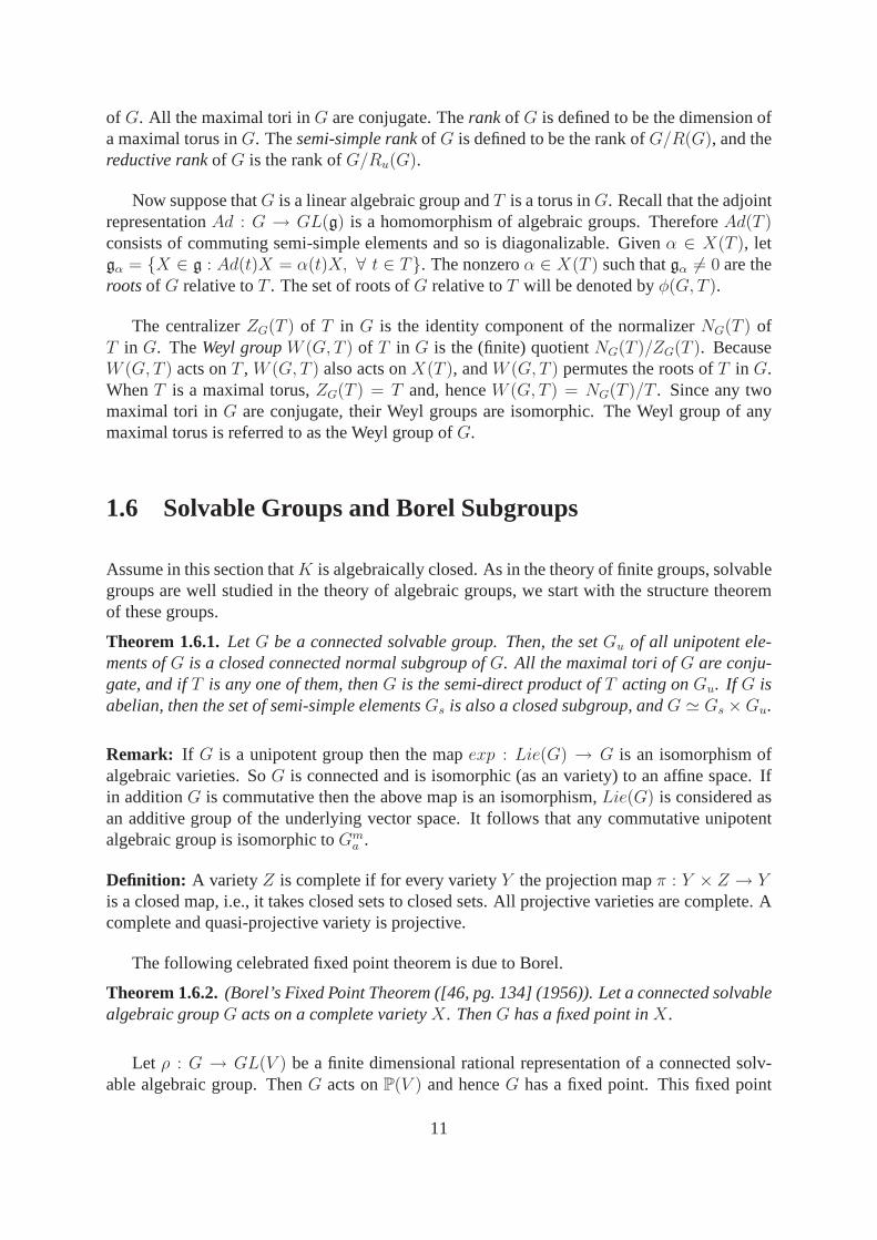
Theorem 1.6.1.Let G be a connected solvable group. Then, the setGu of all unipotent ele-ments ofG is a closed connected normal subgroup ofG. All the maximal tori ofG are conju-gate, and ifT is any one of them, thenG is the semi-direct product ofT acting onGu. If G isabelian, then the set of semi-simple elementsGs is also a closed subgroup, andG ≃ Gs × Gu.

Remark: If G is a unipotent group then the mapexp : Lie(G) → G is an isomorphism ofalgebraic varieties. SoG is connected and is isomorphic (as an variety) to an affine space. Ifin additionG is commutative then the above map is an isomorphism,Lie(G) is considered asan additive group of the underlying vector space. It followsthat any commutative unipotentalgebraic group is isomorphic toGm

a .

Definition: A varietyZ is complete if for every varietyY the projection mapπ : Y × Z → Yis a closed map, i.e., it takes closed sets to closed sets. Allprojective varieties are complete. Acomplete and quasi-projective variety is projective.

The following celebrated fixed point theorem is due to Borel.

Theorem 1.6.2.(Borel’s Fixed Point Theorem ([46, pg. 134] (1956)). Let a connected solvablealgebraic groupG acts on a complete varietyX. ThenG has a fixed point inX.

Let ρ : G → GL(V ) be a finite dimensional rational representation of a connected solv-able algebraic group. ThenG acts onP(V ) and henceG has a fixed point. This fixed point

11

corresponds to aG-stable lineL in V , andG acts onL via some characterχ of G. So, we have;

Theorem 1.6.3.(Lie-Kolchin Theorem ([46, pg. 113]) (1948)). LetG be a connected solvablealgebraic group andρ : G → GL(V ) be a rational representation. Then there is a non-zerovectorv ∈ V such thatρ(g)v = χ(g)v for someχ ∈ X(G) and anyg ∈ G.

Note that the above theorem is analogous to Lie’s theorem fora solvable Lie algebra, whichsays that ifg is a solvable Lie subalgebra ofgl(V ), V finite dimensional, thenV contains acommon eigen vector for all the endomorphisms ing.

Again letG be a connected solvable algebraic group and letρ : G → GL(V ) be a rationalrepresentation. Since the flag varietyF(V ) of complete flags inV is projective, the naturalaction ofG onF(V ) has a fixed point. By taking a basis inV compatible with aG-fixed flagwe haveAρ(G)A−1 ⊆ Tn, for someA ∈ GL(V ), n = dimV .

A Borel subgroupof an algebraic groupG is a connected solvable subgroup ofG which ismaximal in the partial order on closed subgroups given by inclusion of subsets.

Let B be a Borel subgroup ofG andB0 be a Borel subgroup of maximal dimension. ByBorel’s fixed point theorem,B has a fixed point onG/B0, or, equivalently, there is ag ∈ Gwith gBg−1 ⊆ B0. By maximality ofB, gBg−1 = B0. Now take two maximal toriT1 andT2

in G. SinceT1 andT2 are connected and solvable, there are Borel subgroupsB1 andB2 withT1 ⊂ B1, T2 ⊂ B2. Since,gB1g

−1 = B2 for someg ∈ G, T1 andT2 are conjugate. Similarlythe maximal unipotent subgroups ofG are all conjugate. So we have;

Theorem 1.6.4. In an algebraic group the maximal tori (resp. Borel subgroups, maximalconnected unipotent subgroups) are conjugate.

Let B be a Borel subgroup of largest possible dimension in an algebraic groupG. ByChevalley’s theorem there exists a rationalG-moduleV and a non-zerov ∈ V such thatB ={g ∈ G : g.v ∈ K.v}. Let F0 be the closed subvariety of the flag varietyF(V ) consistingof complete flags with the first elementK.v. The subvarietyF0 is B-invariant, and by Borel’sfixed point theoremB has a fixed pointF ∈ F0. Hence the stabilizerGF = B and theG-orbitof F is closed inF(V ), since it is of minimal dimension. So,G/B ≃ G.F is closed in theprojective varietyF(V ), thus is projective too. This gives the following importanttheorem;

Theorem 1.6.5.LetG be an algebraic group andB a Borel subgroup ofG. Then the homoge-neous spaceG/B is projective.

The following theorem shows that conjugates ofB cover the whole groupG.

Theorem 1.6.6.Let B be a Borel subgroup of a connected algebraic groupG, thenG =∪g∈GgBg−1, NG(B) = B, Z(B) = Z(G)0. Further if B is nilpotent, thenB = G. Inparticular G is nilpotent.

A parabolicsubgroupP of G is any closed subgroup ofG such thatG/P is a projectivevariety. LetB be a Borel subgroup ofG. It acts onG/P with a fixed point, sayBgP = gP .

12

This implies thatg−1Bg ⊆ P , i.e., P contains a Borel subgroup. Conversely, supposePcontains a Borel subgroupB. Then the mapG/B → G/P is surjective and,G/B is complete.This shows, the varietyG/P is complete and quasi-projective. So,G/P is projective.

Let P be a parabolic subgroup ofG. ThenP contains a Borel subgroupB of G. Letx ∈ NG(P ). Then bothB andxBx−1 are Borel subgroups ofP 0, so they are conjugate byan elementy ∈ P 0 and henceyx ∈ NG(B) = B. Thusx ∈ P 0, i.e., P 0 = P = NG(P ).So the parabolic subgroups are self-normalizing, connected. Further, ifP, Q are two conjugateparabolic subgroups ofG containing a Borel subgroupB, thenP = Q.

1.7 Root Systems and Semi-simple Theory

An abstract root system in a Euclidean space (a finite dimensional vector space overR endowedwith a positive definite symmetric bilinear form(·, ·) ) V , is a subsetΦ of V that satisfies thefollowing axioms:

(R1): Φ is finite,Φ spansV and0 /∈ Φ.

(R2): If α ∈ Φ, then there exists a reflectionsα relative toα such thatsα(Φ) ⊂ Φ. (Areflection relative toα is a linear transformation sendingα to −α that restricts to the identitymap on a subspace of co-dimension one).

(R3): If α, β ∈ Φ, thensα(β) − β is an integer multiple ofα.

A root system isreducedif it has the property that ifα ∈ Φ, then+α are the only multiplesof α which belong toΦ. The rank ofΦ is defined to bedim(V ). The abstract Weyl groupW (Φ) is the subgroup ofGL(V ) generated by the set{sα : α ∈ Φ}. Note thatW (Φ) is finite,since it permutes the finite setΦ.

Example: Let G be a connected reductive group. LetT be a torus inG and letΦ = Φ(G, T ).Let ZΦ be the subgroup ofX(T ) generated byΦ and letV = ZΦ ⊗Z R. Then the setΦis a subset of the vector spaceV and is a root system. IfT is a maximal torus inG, thenΦ = Φ(G, T ) is a root system inV = ZΦ⊗Z R, and it is reduced. The rank ofΦ is equal to thesemi-simple rank ofG, and the abstract Weyl groupW (Φ) is isomorphic toW = W (G, T ).

A base ofΦ is a subset∆ = {α1, · · · , αl}, such that∆ is a basis ofV and eachα ∈ Φ isuniquely expressed in the formα =

∑li=1 ciαi, where theci’s are all integers, no two of which

have different signs. The elements of∆ are called simple roots andCard(∆) is therankof Φ.The set of positive rootsΦ+ is the set ofα ∈ Φ such that the coefficients of the simple roots inthe expression forα as a linear combination of simple roots, are all nonnegative. Similarly,Φ−

consists of thoseα ∈ Φ such that the coefficients are all non-positive. ClearlyΦ is the disjointunion ofΦ+ andΦ−. Givenα ∈ Φ, there exists a base∆ containingα. Given a base∆, the set{sα : α ∈ ∆} generatesW = W (Φ). The reflectionssα, α ∈ ∆ are called simple reflections.For simplicity we setsi = sαi

, 1 ≤ i ≤ l. The length function onW relative tos1, s2, · · · , sl

13

is given byl(w) = min{k : w = si1si2 · · · sik , 1 ≤ i1, · · · , ik ≤ l}.

If w = si1si2 · · · sik with k = l(w), this is called areduced expressionfor w. There is a uniqueelementw0 of largest length inW , called thelongest elementof W . The elementw0 has theproperty thatw0(α) < 0 for all α > 0, i.e.,w0(Φ

+) = Φ−. There is a partial order inW , calledtheBruhat order, with w′ ≤ w if there exists a sequence{αii, · · · , αik} of simple reflectionssuch thatw′αii · · ·αik = w.

If α, β ∈ Φ, thensα(β) = β − (2(β, α)/(α, α))α. A Weyl chamberin V is a connectedcomponent in the complement of the union of the hyperplanes orthogonal to the roots. The setof Weyl chambers inV and the set of bases ofΦ correspond in a natural way, andW permuteseach of them simply transitively.

If α ∈ Φ, defineα∨ = 2α/(α, α). The setΦ∨ of elementsα∨ (called co-roots) forms a rootsystem inV , called the dual ofΦ. The Weyl groupW (Φ∨) is isomorphic toW (Φ), via the mapsα 7→ s∨α.

A root systemΦ is said to be irreducible ifΦ cannot be expressed as the union of twomutually orthogonal proper subsets. In general,Φ can be partitioned uniquely into a union ofirreducible root systems in subspaces of V.

Let Φ be a root system in an Euclidean spaceV with Weyl groupW . Let

Λ = {λ ∈ V : 〈λ, α〉 := 2(λ, α)/(α, α) ∈ Z, α ∈ Φ}.

Then Λ is a lattice (abelian subgroup generated by a basis ofV ) called weight lattice andelements ofΛ are called weights. Note thatΛ containsΦ. Let Λr be the lattice generated byΦ, called root lattice. Fix a basis∆ of Φ. An elementλ ∈ Λ is called dominant if〈λ, α〉 ≥ 0,∀α ∈ ∆ and strongly dominant if〈λ, α〉 > 0, ∀α ∈ ∆. We denote byΛ+ the set of dominantweights. Each weight is conjugate underW to one and only one dominant weight. Ifλ isdominant, thenσ(λ) ≤ λ, for all σ ∈ W . Moreover forλ ∈ Λ+ the number of dominantweightsµ < λ is finite.

Let ∆ = {α1, α2, · · · , αl}, then the vectors2αi/(αi, αi) also form a basis ofV . Let1, 2, · · · , l be the dual basis, i.e.,2(i, αj)/(αi, αi) = δij . Note thati’s are dom-inant weights called fundamental dominant weights. Every elementλ ∈ V can be writ-ten asλ =

∑mii, wheremi = 〈λ, αi〉. Therefore,Λ = Z1 ⊕ · · ·⊕Zl and Λ+ =

Z≥01 ⊕ · · · ⊕ Z≥0l. SinceΛ andΛr are of same rank, the groupΛ/Λr is a finite group,called thefundamental groupof Φ. The set of fundamental weights and the associated funda-mental group for each type of simple Lie algebras are listed in appendix-B.

1.7.1 Classification of Root Systems

Let (V, Φ) be a root system and let∆ = {α1, · · · , αl} be a base ofΦ. The Cartan matrixA = (ai,j)1≤i,j≤l is the matrix withai,j = 〈αi, α

∨j 〉, where〈α, β∨〉 := 2(β, α)/(α, α). Since

14

all the bases are conjugate under the action ofW , the Cartan matrix is an invariant of the rootsystem (up to simultaneous permutation of rows/columns). Here are some basic propertiesabout this matrix:

(C1)ai,i = 2.

(C2) Fori 6= j, ai,j ∈ {0,−1,−2,−3}.

(C3)ai,j = 0 if and only if aj,i = 0.

We can completely recover the form〈·, ·〉 on V up to a scalar multiple from the Cartanmatrix. We can also recoverΦ since the Cartan matrix contains enough information to com-pute the reflectionsαi

for eachi = 1, · · · , l andΦ = W.∆. So an irreducible root system iscompletely determined up to isomorphism by its Cartan matrix.

A convenient shorthand for Cartan matrices is given by the Dynkin diagram. This is a graphwith vertices labelled byα1, · · · , αl. There areai,j.aj,i edges joining verticesαi andαj , withan arrow pointing towardsαi if (αi, αi) < (αj , αj) (equivalently,ai,j = −1, aj,i = −2,−3).Clearly the Cartan matrix, hence the root system can be recovered from the Dynkin diagram.Now we have a classification theorem for root systems.

Theorem 1.7.1.If Φ is an irreducible root system of rankl, then its Dynkin diagram is one ofthe following:

1 2 3 n−1 n:An (n > 1)

1 2 3 n−1 n( n > :3 )Bn

1 2 3 n−1 n( n > :3 )Cn

1 2 3 n−3 n−2

n−1

n

Dn (n > 4 ) :

1:

6543

2

6E

15

1:

6543

2

E7

7

1 6543

2

E7 8

:8

1 2 3 4:F4

21G 2

:

1.7.2 Classification of Semi-simple Lie Algebras and Algebraic Groups

First we start with a semi-simple Lie algebra and build a rootsystem out of it, and vice versa.Let us begin with a finite dimensional semi-simple Lie algebra g over an algebraically closedfield K. Theng possesses a non-degenerate invariant symmetric bilinear form κ(X, Y ) =Tr(adXadY ) called the Cartan Killing form, where invariant here meansκ([X, Y ], Z) =κ(X, [Y, Z]). Note that ifg is simple, there is a unique such form upto a non-zero scalar.

A maximal toral subalgebrah of g (also called theCartan subalgebra) is a maximal abeliansubalgebra, all of whose elements are semi-simple. It turnsout that in a semi-simple Lie alge-bra, maximal toral subalgebras are non-zero, and they are all conjugate under automorphismsof g. Now fix a maximal toral sub-algebrah. Firstly, the restriction of the invariant formκ ong to h is still non-degenerate. So we can define a map

h∗ → h, α 7→ tα,

wheretα ∈ h is the unique element satisfyingκ(tα, h) = α(h) for all h ∈ h. Now we can evenlift the non-degenerate form onh to h∗, by defining(α, β) = κ(tα, tβ).

Forα ∈ h∗, define

gα = {X ∈ g|[h, X] = α(h)X for everyh ∈ h}.

16

Clearly,g = h⊕αgα. SetΦ = {0 6= α ∈ h∗ : gα 6= 0}. Then we have the Cartan decompositionof g:

g = h ⊕⊕

α∈Φ

gα.

Thegα are one dimensional andΦ satisfies all the properties of a root system. LetV be the realvector subspace ofh∗ spanned byΦ. The restriction of the form onh∗ to V turns out to be realvalued, and makesV into a Euclidean space.

Now start with a reduced root systemΦ and choose a basis∆ = {α1, α2, · · · , αl} of Φ. Foreachi ∈ {1, 2 · · · , l} we associate three symbolsxi, yi, hi and letg be the free Lie algebra withgeneratorsxi, yi, hi (i ∈ {1, 2 · · · , l}). Consider the idealI of g generated by[hihj ], [xiyi] −hi, [xiyj] (i 6= j), [hixj ] − 〈αj, αi〉xj , [hiyj] + 〈αj, αi〉yj, (ad(xi))

−〈αj ,αi〉+1(xj)(i 6= j) and(ad(yi))

−〈αj ,αi〉+1(yj)(i 6= j) and defineg = g/I. It turns out that the Lie algebrag is semi-simple and has root system isomorphic to the givenΦ. The above relations ing among thegenerators are called Chevalley-Serre generators and relations. Now we have a map from thecategory of semi-simple Lie algebras to the set of Dynkin Diagrams (root systems) and viceversa. So we have;

Theorem 1.7.2.The map from semi-simple Lie algebras to Dynkin diagrams gives a bijectionbetween isomorphism classes of semi-simple Lie algebras and Dynkin diagrams. The decom-position of a semi-simple Lie algebra as a direct sum of simple Lie algebras corresponds to thedecomposition of the Dynkin diagram into connected components.

Assume that the ground field is of characteristic0. Then a connected algebraic groupG issemi-simple if and only ifg is semi-simple. In that case,Ad G = G/Z(G). Note that for semi-simpleG, Z(G) is finite. So theorem (1.7.2) almost classifies the semi-simple algebraic groupsin characteristic0: the isomorphism type ofG/Z(G) at least is classified by the isomorphismtype ofg. Since the latter are classified by Dynkin diagrams, so are the centerless semi-simplegroups.

Recall that ifg is simple thenG is simple over an arbitrary field. ButSLn in characteristicdividing n gives us an example whereG is simple butg is not. So theorem (1.7.2) is not true inpositive characteristic.

The following theorem classifies semi-simple algebraic groups in terms of fundamentalgroups.

Theorem 1.7.3.([46, pg. 196]). IfG andG′ are simple algebraic groups having isomorphicroot systems and isomorphic fundamental groups, thenG and G′ are isomorphic, unless theroot system isDl (l ≥ 6) and the fundamental group has order2, in which case there may betwo distinct isomorphic types.

Remark: The groupG is simple (or almost simple) ifG contains no proper nontrivial closedconnected normal subgroup, equivalentlyg is a simple Lie algebra. Note that a simple algebraicgroupG may contain a proper normal subgroup. For example takeSL2 butG/Z(G) is simple

17

as an abstract group. WhenG is semi-simple and connected, thenG is simple if and only ifΦis irreducible.

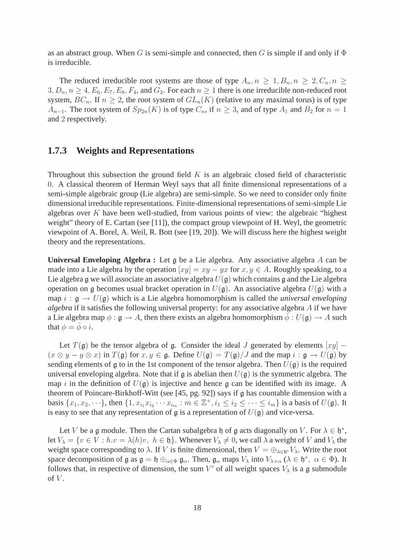
The reduced irreducible root systems are those of typeAn, n ≥ 1, Bn, n ≥ 2, Cn, n ≥3, Dn, n ≥ 4, E6, E7, E8, F4, andG2. For eachn ≥ 1 there is one irreducible non-reduced rootsystem,BCn. If n ≥ 2, the root system ofGLn(K) (relative to any maximal torus) is of typeAn−1. The root system ofSp2n(K) is of typeCn, if n ≥ 3, and of typeA1 andB2 for n = 1and2 respectively.

1.7.3 Weights and Representations

Throughout this subsection the ground fieldK is an algebraic closed field of characteristic0. A classical theorem of Herman Weyl says that all finite dimensional representations of asemi-simple algebraic group (Lie algebra) are semi-simple. So we need to consider only finitedimensional irreducible representations. Finite-dimensional representations of semi-simple Liealgebras overK have been well-studied, from various points of view: the algebraic “highestweight” theory of E. Cartan (see [11]), the compact group viewpoint of H. Weyl, the geometricviewpoint of A. Borel, A. Weil, R. Bott (see [19, 20]). We willdiscuss here the highest weighttheory and the representations.

Universal Enveloping Algebra : Let g be a Lie algebra. Any associative algebraA can bemade into a Lie algebra by the operation[xy] = xy − yx for x, y ∈ A. Roughly speaking, to aLie algebrag we will associate an associative algebraU(g) which containsg and the Lie algebraoperation ong becomes usual bracket operation inU(g). An associative algebraU(g) with amapi : g → U(g) which is a Lie algebra homomorphism is called theuniversal envelopingalgebraif it satisfies the following universal property: for any associative algebraA if we havea Lie algebra mapφ : g → A, then there exists an algebra homomorphismφ : U(g) → A suchthatφ = φ ◦ i.

Let T (g) be the tensor algebra ofg. Consider the idealJ generated by elements[xy] −(x ⊗ y − y ⊗ x) in T (g) for x, y ∈ g. DefineU(g) = T (g)/J and the mapi : g → U(g) bysending elements ofg to in the 1st component of the tensor algebra. ThenU(g) is the requireduniversal enveloping algebra. Note that ifg is abelian thenU(g) is the symmetric algebra. Themap i in the definition ofU(g) is injective and henceg can be identified with its image. Atheorem of Poincare-Birkhoff-Witt (see [45, pg. 92]) says if g has countable dimension with abasis{x1, x2, · · ·}, then{1, xi1xi2 · · ·xim : m ∈ Z+, i1 ≤ i2 ≤ · · · ≤ im} is a basis ofU(g). Itis easy to see that any representation ofg is a representation ofU(g) and vice-versa.

Let V be ag module. Then the Cartan subalgebrah of g acts diagonally onV . Forλ ∈ h∗,let Vλ = {v ∈ V : h.v = λ(h)v, h ∈ h}. WheneverVλ 6= 0, we callλ a weight ofV andVλ theweight space corresponding toλ. If V is finite dimensional, thenV = ⊕λ∈h∗Vλ. Write the rootspace decomposition ofg asg = h ⊕α∈Φ gα. Then,gα mapsVλ into Vλ+α (λ ∈ h∗, α ∈ Φ). Itfollows that, in respective of dimension, the sumV ′ of all weight spacesVλ is ag submoduleof V .

18

Choose a basis∆ = {α1, α2, · · · , αl} of Φ. A maximal vector (of weightλ) in ag-moduleV is a non-zero vectorv+ ∈ Vλ such thatgα.v+ = 0 (α ∈ ∆). If dim(V ) is finite, then theBorel subalgebrab(∆) := h⊕α>0 gα has a common eigen vector by Lie’e theorem, and this isa maximal vector inV .

In order to study finite dimensional irreducibleg-modules, it is useful to study first the largerclass ofg-modules generated by a maximal vector. IfV = U(g).v+ for a maximal vectorv+

(of weightλ), we say thatV is standard cyclic(of weightλ) and we callλ thehighest weightof V . In this caseV is the direct sum of its weight spaces and the weights are of the formµ = λ −

∑li=1 kiαi (ki ∈ Z≥0). This justifies the terminology highest weight forλ, since

µ ≤ λ. Again V is an indecomposableg-module, with a unique proper maximal submoduleand a corresponding unique irreducible quotient. If further, V itself was irreducible, thenv+ isthe unique maximal vector inV , up to non-zero scalar multiples. It is easy to check that such acyclic module is unique upto isomorphism if it exists.

For the existence, there are two ways to construct a cyclicg-module of highest weightλ foranyλ ∈ h∗. The first way of construction is to consider the one dimensional vector spaceDλ =K.v+ and define an action ofb = b(∆) = h ⊕α>0 gα onDλ by h.v+ = λ(h)v+, xα.v+ = 0.Consider theU(g)-moduleZ(λ) = U(g) ⊗U(b) Dλ. Then,Z(λ) is a standard cyclic module ofweightλ and the element1 ⊗ v+ is a highest weight vector of weightλ (see [45, Ch. 6]). Theother way of construction is the Verma module. Consider the left idealI(λ) in U(g) generatedby {xα, α ∈ Φ+} and{hα − λ(hα).1, α ∈ Φ}. ThenU(g)/I(λ) is ag-module with highestweight λ. There is a canonical homomorphism of leftU(g)-modulesU(g)/I(λ) → Z(λ)sending the coset of 1 onto the maximal vectorv+. Again using PBW basis ofU(g) it is easy tosee that the above map is infact an isomorphism. The standardcyclic moduleZ(λ) of weightλ has a unique maximal submoduleY (λ) and therefore,V (λ) = Z(λ)/Y (λ) is an irreduciblestandard cyclicg-module of weightλ.

We now discuss the following: (1) For whichλ, theV (λ) are finite dimensional. (2) De-termine for suchV (λ), exactly which weightsµ occur and give the formula for multiplicity ofV (λ)µ in V (λ).

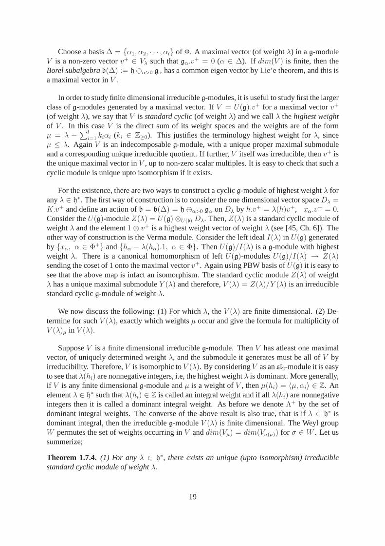
SupposeV is a finite dimensional irreducibleg-module. ThenV has atleast one maximalvector, of uniquely determined weightλ, and the submodule it generates must be all ofV byirreducibility. Therefore,V is isomorphic toV (λ). By consideringV as ansl2-module it is easyto see thatλ(hi) are nonnegative integers, i.e, the highest weightλ is dominant. More generally,if V is any finite dimensionalg-module andµ is a weight ofV , thenµ(hi) = 〈µ, αi〉 ∈ Z. Anelementλ ∈ h∗ such thatλ(hi) ∈ Z is called an integral weight and if allλ(hi) are nonnegativeintegers then it is called a dominant integral weight. As before we denoteΛ+ by the set ofdominant integral weights. The converse of the above resultis also true, that is ifλ ∈ h∗ isdominant integral, then the irreducibleg-moduleV (λ) is finite dimensional. The Weyl groupW permutes the set of weights occurring inV anddim(Vµ) = dim(Vσ(µ)) for σ ∈ W . Let ussummerize;

Theorem 1.7.4.(1) For anyλ ∈ h∗, there exists an unique (upto isomorphism) irreduciblestandard cyclic module of weightλ.

19

(2) If λ ∈ h∗ is dominant integral, then the irreducibleg-moduleV (λ) is finite dimensional.

(3) Every finite dimensional irreducibleg-moduleV is isomorphic toV (λ) for some domi-nant integral weightλ.

(4) The Weyl groupW permutes the set of weights occurring inV anddim(Vµ) = dim(Vσ(µ))for σ ∈ W .

Corollary 1.7.5. The mapλ 7→ V (λ) induces a one-one correspondence betweenΛ+ and theisomorphism classes of finite dimensional irreducibleg-modules.

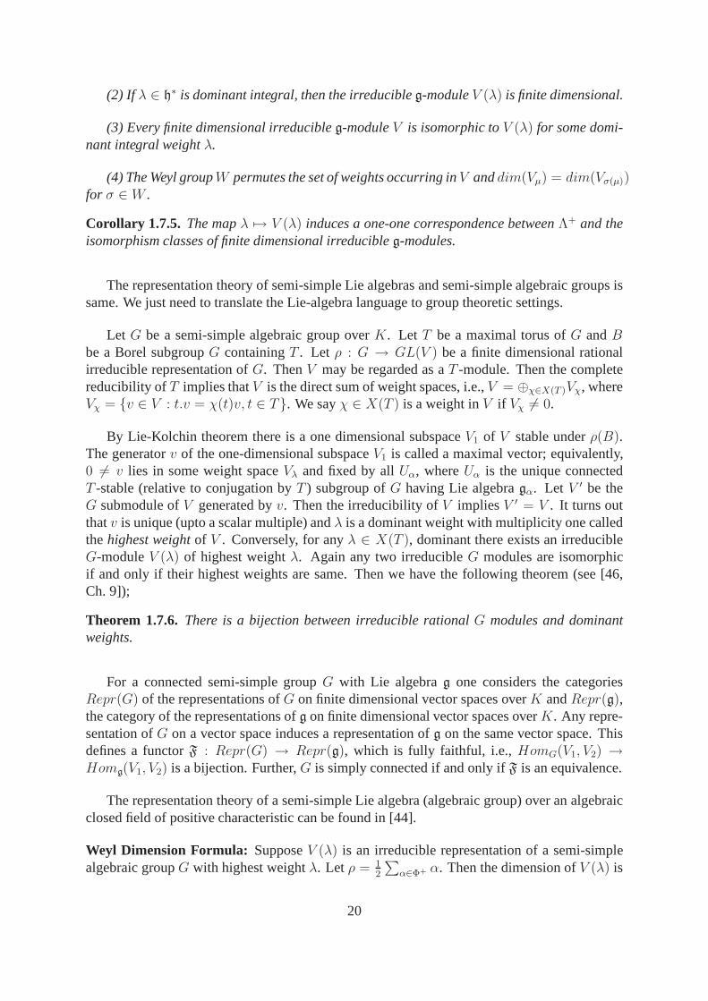
The representation theory of semi-simple Lie algebras and semi-simple algebraic groups issame. We just need to translate the Lie-algebra language to group theoretic settings.

Let G be a semi-simple algebraic group overK. Let T be a maximal torus ofG andBbe a Borel subgroupG containingT . Let ρ : G → GL(V ) be a finite dimensional rationalirreducible representation ofG. ThenV may be regarded as aT -module. Then the completereducibility ofT implies thatV is the direct sum of weight spaces, i.e.,V = ⊕χ∈X(T )Vχ, whereVχ = {v ∈ V : t.v = χ(t)v, t ∈ T}. We sayχ ∈ X(T ) is a weight inV if Vχ 6= 0.

By Lie-Kolchin theorem there is a one dimensional subspaceV1 of V stable underρ(B).The generatorv of the one-dimensional subspaceV1 is called a maximal vector; equivalently,0 6= v lies in some weight spaceVλ and fixed by allUα, whereUα is the unique connectedT -stable (relative to conjugation byT ) subgroup ofG having Lie algebragα. Let V ′ be theG submodule ofV generated byv. Then the irreducibility ofV impliesV ′ = V . It turns outthatv is unique (upto a scalar multiple) andλ is a dominant weight with multiplicity one calledthehighest weightof V . Conversely, for anyλ ∈ X(T ), dominant there exists an irreducibleG-moduleV (λ) of highest weightλ. Again any two irreducibleG modules are isomorphicif and only if their highest weights are same. Then we have thefollowing theorem (see [46,Ch. 9]);

Theorem 1.7.6.There is a bijection between irreducible rationalG modules and dominantweights.

For a connected semi-simple groupG with Lie algebrag one considers the categoriesRepr(G) of the representations ofG on finite dimensional vector spaces overK andRepr(g),the category of the representations ofg on finite dimensional vector spaces overK. Any repre-sentation ofG on a vector space induces a representation ofg on the same vector space. Thisdefines a functorF : Repr(G) → Repr(g), which is fully faithful, i.e.,HomG(V1, V2) →Homg(V1, V2) is a bijection. Further,G is simply connected if and only ifF is an equivalence.

The representation theory of a semi-simple Lie algebra (algebraic group) over an algebraicclosed field of positive characteristic can be found in [44].

Weyl Dimension Formula: SupposeV (λ) is an irreducible representation of a semi-simplealgebraic groupG with highest weightλ. Let ρ = 1

2

∑

α∈Φ+ α. Then the dimension ofV (λ) is

20

given by

dim(V (λ)) =

∏

α∈Φ+〈α, λ + ρ〉∏

α∈Φ+〈α, ρ〉.

Weyl Character Formula: Sometimes it is convenient to write the elements ofX(T ) multi-plicatively. So, we introduce symbolseλ for λ ∈ X(T ) subject to the ruleeλ.eµ = eλ+µ. Thecharacter of an irreducible representationV (λ) is given by

ch(V (λ)) =

∑

w∈W (−1)l(w)(ew(λ+ρ))

eρ∏

α∈Φ+(1 − e−α).

Kostant Multiplicity Formula: Supposeµ is an element of the root lattice. Letp(µ) denotethe number of ways thatµ can be expressed as a linear combination of positive roots withnon-negative integer co-efficients. The functionp is called theKostant partition function.

Suppose thatV (λ) is a finite dimensional irreducible representation of a semi-simple alge-braic groupG with highest weightλ. If µ is a weight ofV (λ), then the multiplicitymµ(λ) isgiven by

mµ(λ) =∑

w∈W

(−1)l(w)p(w.(λ + ρ) − (µ + ρ)).

1.8 Reductive Group

Recall that, a linear algebraic groupG is said to be reductive if its unipotent radicalRu(G) istrivial. If G is connected, thenR(G) is a torus. The following theorem reduces the study ofreductive groups to the study of semi-simple groups and tori.

Theorem 1.8.1.Let G be a connected reductive algebraic group. Then we haveR(G) =Z(G)0, G = R(G)[G, G], and the subgroup[G, G] is semi-simple.

Let G be a connected reductive group. LetT be a torus inG. ThenZG(T ) is reductive.This fact is useful for inductive arguments. Let〈Φ〉 be the subgroup ofX(T ) generated byΦand letV = 〈Φ〉 ⊗Z R. Then the setΦ is a subset of the vector spaceV and is a root system. IfT is a maximal torus, then the root system is reduced. The rank of Φ is equal to the semi-simplerank ofG, and the abstract Weyl groupW (Φ) is isomorphic toW = W (G, T ).

Now let us assume thatT is a maximal torus. Lett be the Lie algebra ofT and letΦ =Φ(G, T ). Then

(1) g = t ⊕⊕

α∈Φ gα anddimgα = 1 for all α ∈ Φ.

(2) If α ∈ Φ, let Tα = (Kerα)0. ThenTα is a torus of co-dimension one inT .

21

(3) If α ∈ Φ, let Zα = ZG(Tα). ThenZα is a reductive group of semi-simple rank 1, andthe Lie algebrazα of Zα satisfieszα = t⊕gα ⊕g−α. The groupG is generated by the subgroupsZα, α ∈ Φ+.

(4) The centreZ(G) of G is equal to∩α∈ΦTα.

(5) If α ∈ Φ, there exists a unique connectedT -stable (relative to conjugation byT ) sub-groupUα of G having Lie algebragα. Also,Uα ⊂ Zα.

(6) Let n ∈ NG(T ), and letw be the corresponding element ofW = W (G, T ). ThennUαn−1 = Uw(α) for all α ∈ Φ.

(7) Let α ∈ Φ. Then there exists an isomorphismǫ : Ga → Uα such thattǫα(x)t−1 =ǫα(α(t)x), t ∈ T, x ∈ Ga.

(8) The groupsUα, α ∈ Φ, together withT , generate the groupG.

The Bruhat Decomposition: Let B be a Borel subgroup ofG, and letT be a maximal torusof G contained inB. ThenG is the disjoint union of the double cosetsBwB, asw ranges overa set of representatives inNG(T ) of the Weyl groupW (BwB = Bw′B if and only if w = w′

in W ), i.e.,G = ⊔w∈W BwB.

Remark: More generally the Bruhat decomposition holds for a group with BN-pair. A BN-pair in a groupG is a datum(B, N, S) consisting of sub-groupsB andN , such thatB ∩ N isnormal inN , and a set of involutionsS in the quotient groupW = N/(B ∩ N). The datumsatisfies the following properties:

(1) The setB ∪ N generatesG.

(2) The setS generatesW .

(3) For anys ∈ S, andw ∈ W we havesBw ⊂ BwB ∪ BswB.

(4) For anys ∈ S we havesBs 6⊂ B.

The groupW is called the Weyl group of theBN-pair (see [3, pg. 15]). It follows fromthese properties that(W, S) is in fact a Coxeter system, and moreover the third property can berefined to

BsBwB =

{BswB if l(sw) = l(w) + 1.BwB ∪ BswB if l(sw) = l(w) − 1.

Let G be a connected reductive group. Then ifB is a Borel subgroup andT is a maximaltorus inB, the pair of subgroupsB andN = NG(T ) is aBN-pair for G, where the setS isequal to{sα : α ∈ ∆} ⊂ W .

22

1.8.1 Classification of Reductive Algebraic Groups

Like semi-simple algebraic groups are classified by root systems, the reductive algebraic groupsare classified by an invariant calledroot datum. An abstract root datumis a quadrupleΨ =(X, Y, Φ, Φ∨), whereX andY are free abelian groups such that there exists a bilinear mapping〈·, ·〉 : X × Y → Z inducing isomorphismsX ≃ Hom(Y, Z) andY ≃ Hom(X, Z), andΦ ⊂ X andΦ∨ ⊂ Y are finite subsets, and there exists a bijectionα 7→ α∨ of Φ ontoΦ∨. Thefollowing two axioms must be satisfied:

(RD1): 〈α, α〉 = 2

(RD2): If sα : X → X andsα∨ : Y → Y are defined bysα(x) = x − 〈x, α∨〉α, andsα∨(y) = y − 〈α, y〉α∨, thensα(Φ) ⊂ Φ and sα∨(Φ∨) ⊂ Φ∨ (for all α ∈ Φ). (see [115,pg. 124])

If Φ 6= ∅, thenΦ is a root system inV = 〈Φ〉 ⊗Z R, where〈Φ〉 is the subgroup ofXgenerated byΦ. The setΦ∨ is the dual of the root system. The quadrupleΨ∨ = (Y, X, Φ∨, Φ)is also a root datum, called the dual ofΨ. A root datum isreducedif it satisfies a third axiom

(RD3): α ∈ Φ ⇒ 2α /∈ Φ.

Let G be a connected reductive group and letT be a maximal torus inG. Then the quadru-ple Ψ(G, T ) = (X, Y, Φ, Φ∨) = (X(T ), Y (T ), Ψ(G, T ), Ψ∨(G, T )) is a root datum and it isreduced.

An isomorphism of a root datumΨ = (X, Y, Φ, Φ∨) onto a root datumΨ′

= (X ′, Y ′, Φ′

, Φ′∨)

is a group isomorphismf : X → X ′ which induces a bijection ofΦ ontoΦ′ and whose dualinduces a bijection ofΦ′∨ ontoΦ∨. If G′ is a linear algebraic group which is isomorphic toG,andT ′ is a maximal torus inG′, then the root dataΨ(G, T ) andΨ(G′, T ′) are isomorphic.

If Ψ is a reduced root datum, there exists a connected reductive group G and a maximaltorusT in G such thatΨ = Ψ(G, T ). The pair(G, T ) is unique up to isomorphism. So wehave (see [115, Ch. 9, 10]);

Theorem 1.8.2.For every root datum, there exists a corresponding reductive algebraic group.Further, any two reductive algebraic groups are isomorphicif and only if their root datums(relative to some maximal tori) are isomorphic.

1.9 Parabolic Subgroups

Recall that a parabolic subgroup of G is a closed subgroupQ of G such thatG/Q is a projectivevariety. Note that a subgroupQ of G is parabolic if and only if it contains a Borel subgroup.

Let Q be a parabolic subgroup containing a Borel subgroupB. Let R(Q) be the radicalof Q, namely, the connected component through the identity element of the intersection of all

23

the Borel subgroups ofQ. Let Ru(Q) be the unipotent radical ofQ and letΦ+Q be the subset

of Φ+ defined byΦ+ \ Φ+Q = {α ∈ Φ+ : Uα ⊂ Ru(Q)}. Let Φ−

Q = −Φ+Q, ΦQ = Φ+

Q ∪ Φ−Q

and∆Q = ∆ ∩ ΦQ. ThenΦQ is a subroot system ofΦ called the root system associated toQ, with ∆Q as a set of simple roots andΦ+

Q (resp.Φ−Q) as the set of positive (resp. negative)

roots ofΦQ relative to∆Q. On the other hand, given a subsetJ of ∆, the subgroupQ of Ggenerated byB andU−α, α ∈ Φ+

J = {∑

β∈J aββ : aβ ≥ 0} ∩ Φ+ is a parabolic subgroupof G containingB. Thus the set of parabolic subgroups containingB is in bijection with thepower set of∆. In particular forQ = B (resp.G), ∆Q is the empty set (resp. the whole set∆).The subgroup ofQ generated byT and{Uα : α ∈ ΦQ} is called theLevi subgroupassociatedto ∆Q, and is denoted byLQ. We have thatQ is the semidirect product ofRu(Q) andLQ

called theLevi decompositionof Q. The set of maximal parabolic subgroups containingB isin one-to-one correspondence with∆. Namely givenα ∈ ∆, the parabolic subgroupQ where∆Q = ∆ \ {α} is a maximal parabolic subgroup, and conversely. We shall denote the maximalparabolic subgroupQ, where∆Q = ∆ \ {αi} by Pi.

1.9.1 The Weyl Group of a Parabolic Subgroup

Given a parabolic subgroupQ, let WQ be the subgroup ofW generated by{sα : α ∈ ∆Q}.WQ is called the Weyl group ofQ. Note thatWQ ≃ NQ(T )/T , whereNQ(T ) is the normalizerof T in Q. In each cosetwWQ ∈ W/WQ, there exists a unique element of minimal length.Let W min

Q be the set of minimal length representatives ofW/WQ . We haveW minQ = {w ∈

W : l(ww′) = l(w) + l(w′), for all w′ ∈ WQ}. In other words, each elementw ∈ W canbe written uniquely asw = uv whereu ∈ W min

Q , v ∈ WQ and l(w) = l(u) + l(v). The setW min

Q can also be characterized asW minQ = {w ∈ W : w(α) > 0, for all α ∈ ∆Q}. W min

Q isalso denoted byW Q. Similarly in each cosetwWQ ∈ W/WQ, there exists a unique elementof maximal length and the setW max

Q of maximal length representatives ofW/WQ is equal to{w ∈ W : w(α) < 0, for all α ∈ ∆Q}. Further if wQ is the unique element of maximallength inWQ, then we haveW max

Q = {wwQ : w ∈ W minQ }. If Q is the parabolic subgroup

corresponding to a subsetI of ∆, thenWQ (resp.W Q) is also denoted byWI (resp.W I).

1.10 Schubert Varieties

Let G be a semi-simple algebraic group over an algebraically closed field K. Let T be amaximal torus ofG andB be a Borel subgroup ofG containingT . The projective varietyG/P is called a generalised flag variety. For the left action ofT on G/P , there are onlyfinitely many fixed points{ew := wWP : w ∈ W/WP}. For w ∈ W/WP , the B-orbitCP (w) := Bew = BwP/P in G/P is a locally closed subset ofG/P , called theSchubertcell. The Zariski closure ofCP (w) with the canonical reduced structure is theSchubert varietyassociated tow, and is denoted byXP (w). Thus Schubert varieties inG/P are indexed byW P . Note that ifP = B, thenWP = {id}, and the Schubert varieties inG/B are indexed bythe elements ofW . We denote the Schubert variety corresponding tow ∈ W by X(w).

24

Dimension ofXP (w): If P = B, then forw ∈ W , the isotropy subgroup inG at theT fixedpoint ew in G/B is wBw−1; hence, the isotropy subgroup in the unipotent radicalBu (of B)at ew is generated by the root subgroups{Uα, α ∈ Φ+ : Uα ⊂ wBw−1}, i.e.,{Uα, α ∈ Φ+ :w−1(α) > 0}. Hence we get an identification

CB(w) ≃∏

{α∈Φ+:w−1(α)<0}

Uα

Since|{α ∈ Φ+ : w−1(α) < 0}| = l(w), CB(w) is isomorphic to the affine spaceK l(w). Hencewe have

dimXB(w) = dimCB(w) = l(w).

For a general parabolicP , considerw ∈ W/WP and denote the unique representativefor w in W min

P (resp. W maxP ) by wmin

P (resp. wmaxP ). Now under the canonical projection

πP : G/B → G/P , XB(wminP ) maps birationally ontoXP (w), andXB(wmax

P ) = π−1P (XP (w)).

Hence we obtaindimXP (w) = dimXB(wmin

P ) = l(wminP ).

Note that,G/B = X(w0), w0 being the longest element inW . The cellCB(w0) is theunique cell of maximal dimension (=l(w0) = |Φ+|); it is affine, open and dense inG/B, calledthebig cell of G/B. It is denoted asO. Let B− = w0Bw−1

0 be the opposite Borel subgroupto B. TheB− orbit B−eid is again affine, open and dense inG/B, and is called theoppositebig cell of G/B, and it is denoted asO−. For aw ∈ W , YB(w) = XB(w) ∩ O− is called theopposite cell inXB(w).

There is a partial order onWP , known as the Bruhat order, induced by the partial orderon the set of Schubert varieties given by inclusion, namely,for w1, w2 ∈ WP , w1 ≥ w2 ⇐⇒XP (w1) ⊇ XP (w2). TakingQ = B, we obtain a partial order onW .

The Bruhat decomposition ofG/P andXP (w) are induced by the Bruhat decomposition ofG/B. They areG/P =

⊔

w∈W P BewP (modP ) andXP (w) =⊔

{w∈W P , ew′∈XP (w)} Bew′P (modP )respectively.

Example: Let G = SLn+1 andP = Pα1. The semi-simple part of thisP is justSLn. Thus

WP = Sn and has the longest element(w0)P = sn(sn−1sn) · · · (s2 · · · sn). Note thatw0 =(w0)P (s1 · · · sn). The number of Schubert varieties inG/P is then[W : WP ] = n + 1. These

are given by the sequencewi =

{id if i = 0;si · · · s1 if 1 ≤ i ≤ n.

1.10.1 Line Bundles on G/P

For the study ofG/B, there is no loss in generality in assuming thatG is simply connected; inparticular, the character groupX(T ) coincides with the weight latticeΛ. Henceforth, we shallsuppose thatG is simply connected. The canonical projectionπ : G → G/B is a principalB-bundle withB as both the structure group and fiber. Anyλ ∈ X(T ) defines a character

25

λB : B → Gm obtained by composing the natural mapB → T with λ : T → Gm. Then wehave an action ofB onK, namelyb.k = λB(b)k, b ∈ B, k ∈ K. SetE = G × K/ ∼, where∼ is the equivalence relation defined by(gb, b.k) ∼ (g, k), g ∈ G, b ∈ B, k ∈ K. ThenE isthe total space of a line bundle overG/B. We denote byL(λ), the line bundle associated toλ.Thus we obtain a map

L : X(T ) → Pic(G/B), λ 7→ L(λ),

wherePic(G/B) is the Picard group ofG/B which is by definition, the group of isomorphismclasses of line bundles onG/B. By a theorem of Chevalley [16] the above map is in fact anisomorphism of groups sinceG is simply connected.

On the other hand, consider the irreducible divisorsX(w0si), 1 ≤ i ≤ l on G/B. LetLi = OG/B(X(w0si)) be the line bundle defined byX(w0si), 1 ≤ i ≤ l. The Picard groupPic(G/B) is a free abelian group generated by theLi’s, and under the isomorphismL :X(T ) ≃ Pic(G/B), we haveL(i) = Li, 1 ≤ i ≤ l (see [16]). Thus forλ =

∑li=1〈λ, αi〉i,

we haveL(λ) = ⊗li=1L

⊗〈λ,αi〉i .

For a general parabolicP , anyλ ∈ X(T ) can not be lifted to a character ofP always. To bea character ofP the weightλ must be orthogonal to the positive roots ofP . Therefore,λ mustbe an integral linear combination of the fundamental weights, 1, · · · , r dual to the simpleroots in∆P . We call1, · · · , r the fundamental weights ofP and the sublatticeΛP ⊂ Λ theygenerate the weights ofP .

A line bundleL on an algebraic varietyX is very ample if there exists an immersioni :X → Pn such thati∗(OPn(1)) = L. A line bundleL on X is ample ifLm is very ample forsome positive integerm ≥ 1. A line bundleL on X is said to benumerically effective, if thedegree of the restriction to any algebraic curve inX is non-negative.

The following theorem summarizes some well-known facts about line bundles onG/P (forexample see [113]).

Theorem 1.10.1.Let X = G/P , whereG is a semi-simple algebraic group and P is aparabolic subgroup. Let 1, · · · , r be the fundamental weights ofP and letL be a linebundle onX defined byλ =

∑rj=1 mjj ∈ ΛP . Then

(1) X = X1 × · · · × Xs, whereXi = Gi/Pi, Gi is a simple algebraic group andPi is aparabolic subgroup ofGi, i = 1, · · · , s.(2)L = pr∗1L1 ⊗ · · · ⊗ pr∗sLs, whereLi is a line bundle onXi, i = 1, · · · , s.(3) Pic(X) ≃ ΛP . In particular,Pic(X) ≃ Z if P is a maximal parabolic subgroup ofG.(4)L is numerically effective if and only ifλ is dominant.(5)L is very ample if and only ifλ is a regular dominant weight (〈λ, αi〉 > 0, for all αi ∈ ∆).

As we have described above, letE denote the total space of the line bundleL(λ), overG/B. Let σ : E → G/B be the canonical mapσ(g, c) = gB. Let

Mλ = {f ∈ K[G] : f(gb) = λ(b)f(g), g ∈ G, b ∈ G}.

ThenMλ can be identified with the space of sectionsH0(G/B, L(λ)) := {s : G/B →E : σ ◦ s = idG/B} as follows. Tof ∈ Mλ, we associate a sections : G/B → E by

26

settings(gB) = (g, f(g)). To see thats is well defined, considerg′ = gb, b ∈ B. Then(g′, f(g′)) = (gb, f(gb)) = (gb, λ(b)f(g)) = (gb, bf(g)) ∼ (g, f(g)). From this, it followsthat s is well defined. Conversely, givens ∈ H0(G/B, L(λ)), considergB ∈ G/B. Lets(gB) = (g′, f(g′)), whereg′ = gb for someb ∈ B (note thatg′B = gB, sinceσ ◦ s = idG/B).Now the point(g′, f(g′)) may also be represented by(g, λ(b)−1f(gb)) (since(g′, f(g′)) =(gb, f(gb)) ∼ (g, λ(b)−1f(gb)). Thus giveng ∈ G, there exists a unique representative of theform (g, f(g)) for s(gB). This defines a functionf : G → K. Further, thisf has the propertythat forb ∈ B, f(g) = λ(b)−1f(gb), i.e.,f(gb) = λ(b)f(g), b ∈ B, g ∈ G. Thus we obtainan identification

Mλ = H0(G/B,L(λ)).

It can be easily verified that the above identification preserves the respectiveG-module struc-tures.

1.10.2 Weyl Module

In this section we assume that the ground field isC. Let G be a semi-simple algebraic groupover C with root systemΦ and the set of simple roots∆. Let g = Lie(G) and letU(g)be the universal enveloping algebra ofg. Let U+(g) be the subalgebra ofU(g) generated by{Xα : α ∈ ∆}, andU+

Z(g) be the KostantZ-form of U+(g), which is by definition theZ-

subalgebra ofU+(g) generated by{Xnα

n!, α ∈ Φ+, n ∈ N}.

Let λ be a dominant weight, andV (λ) be the irreducibleG-module overC. Fix a highest-weight vectoruλ in V of weightλ; we have that the weightλ in V (λ) has multiplicity one. Forw ∈ W , fix a representativenw for w in NG(T ), and setuw,λ = nwuλ, known as anextremalweight vector; it is a weight vector inV (λ) of weightw(λ), and is unique up to scalars. Havingfixedλ, we shall denoteuλ (resp.uwλ) by justu (resp.uw ). SetVw,Z(λ) = U+

Z(g)uw. For any

field K, let Vw,λ = Vw,Z(λ) ⊗ K, w ∈ W . ThenVK(λ) := Vw0,λ = Vw0,Z(λ) ⊗ K is theWeylmodulewith highest weightλ, and forw ∈ W , Vw,λ is theDemazure modulecorresponding tow andλ (see [72, pg. 25]). The vectorsuw,λ for w ∈ W are also called extremal weight vectorsin VK(λ). Then the following theorem can be found in [49].

Theorem 1.10.2.H0(G/B,L(λ)) ≃ VK(λ)∗ andH0(X(w),L(λ)) ≃ V ∗w,λ.

27

Chapter 2

Invariant theory

This chapter is a brief survey of invariant theory of finite groups as well as reductive algebraicgroups. Here we present many classical as well as modern results in invariant theory mostlyon computational aspects. In the last section of this chapter “Geometric invariant theory” isintroduced.

2.1 Introduction

Invariant theory served as one of the major motivations for the development of commutative al-gebra: from Hilbert’s basis theorem to Noetherian rings andmodules. It is primarily concernedwith the study of group actions, their fixed points and their orbits. The actions are usually onalgebras of various sorts, the fixed points are subalgebra, and the orbits form a variety of groupson rings and the invariants of the action, e.g. the fixed subring and related objects. The basicobject to study is the ring of invariants. In this chapter we deal with only linear actions. IfG is afinite group acting linearly on a vector spaceV over a fieldK, then the action may be extendedto K[V ], the algebra of polynomial functions onV , by the formula(gf)(v) := f(g−1.v) for allv ∈ V and the ring ofG-invariant polynomials isK[V ]G := {f ∈ K[V ] : gf = f ∀ g ∈ G}. IfG is a linear algebraic group acting on an affine varietyX, then the same formula above definesan action on the coordinate ringK[X] of X andK[X]G := {f ∈ K[X] : gf = f ∀ g ∈ G}.In this section we focus on the case whenX = V is a representation ofV and, when we talkabout algebraic group actions, the base fieldK is algebraic closed, unless stated otherwise. TheG action onK[V ] preserves degree andK[V ]G ⊆ K[V ] inherits the grading.

The basic question in invariant theory is when isK[V ]G finitely generated ? If it is finitelygenerated then find the generators and relations forK[V ]G(fundamental systems of invariants),find the degree bounds for the generators. When isK[V ]G a polynomial ring ? If not thenwhat is the distance ofK[V ]G from being a polynomial ring ? and, what is the distance ofK[V ]G from being free as module over a homogeneous system of parameters ? What is thecohomological co-dimension:depth(K[V ]G) ?

28

2.2 Finite Generation

The question, whether there is always a finite set of fundamental invariants for arbitrary groupswas considered to be one of the most important problems in 19’th century algebra. It wasproved to be true, using explicit calculations, by P Gordan for K = C andG = SL2(C) inthe 1860/70’s. In 1890 David Hilbert introduced new methodsin invariant theory, which stilltoday are basic tools of modern algebra (Hilbert’s basis theorem). Applying these he was ableto prove finite generation for the invariants of the general linear groupsGLn(C).

In the year 1900, on the occasion of the international congress of mathematics in Paris,Hilbert posed the general question of finite generation of invariant rings for arbitrary groupsas the 14’th of the now famous “Hilbert problems”. In generalthe answer to this question isnegative: In 1958 Nagata gave a counterexample to this.

For finite groups, Hilbert’s 14’th problem has been solved affirmatively: In 1916 EmmyNoether had considered the problem specifically forK = C, where she was able to find con-structive procedures to compute fundamental systems explicitly. Ten years later (1926) sheproved that the invariant ring is finitely generated, ifG is a finite group andK is an arbitraryfield. The price one has to pay for this generality is, that theproof is not constructive and doesnot provide an immediate algorithm how to compute a finite setof fundamental invariants.

Theorem 2.2.1.(Hilbert [40], 1890; Noether [88, 89], 1916, 1926). Let G be afinite group.Then the ring extensionK[V ]G ⊆ K[V ] is finite andK[V ]G is a finitely generatedK-algebra.

In the general setting, finite generation no longer holds forK[V ]G. There are many counterexamples. This is the Nagata’s famous counter example to Hilbert’s 14’th problem.

Nagata’s counter example [79]: Let G′ be the subgroup ofGna equal to the set of solutions

(t1, · · · , tn) of a system of linear equations∑n

j=1 aijxj = 0, i = 1, 2, 3. The groupG′ acts onthe affine spaceC2n by the formula(t1, · · · , tn)(x1, y1, · · · , xn, yn) = (x1 + t1y1, y1, · · · , xn +tnyn, yn). Now consider the subgroupH = {(h1, · · · , hn) ∈ Gn

a :∏n

i=1 hi = 1} of Gnm. It

acts onC2n by the formula(h1, · · · , hn).(x1, y1, · · · , xn, yn) = (h1x1, h1y1, · · · , hnxn, hnyn).Both of these groups are identified naturally with subgroupsof SL2n and we enlargeG′ byconsidering the groupG = G′H. Then Nagata showed that, in an appropriate choice ofaij ’sand the numbern the algebra of invariantsK[x1, · · · , xn, y1, · · · , yn]

G is not finitely generated.For example, takingn = 16 and aij ’s are algebraically independent overQ, the invariantalgebra is not finitely generated (see [22, pg. 43]).

Remark: Here are some more counter examples involving the additive groupGa. LetK be analgebraically closed field of characteristic0. Roberts [94] found a non-linear action ofGa onK7 such that the invariant ring is not finitely generated. Recently, Daigle and Freudenburg [18]found the following counter example in dimension 5. Consider the action ofGa onK5 definedby g.(a, b, x, y, z) = (a, b, x + ga2, y + g(ax + b) + 1

2g2a3, z + gy + 1

2g2(ax + b) + 1

6g3a3).

ThenC[a, b, x, y, z]Ga is not finitely generated. However forn ≤ 3, Zariski [125] showed thatfor any rational action ofGa on Kn that the invariant ring is finitely generated and ifV is a

29

representation ofGa over a fieldK of characteristic0, Weitzenbock [122] proved thatK[V ]G

is finitely generated.

Reductivity, Linear Reductivity and Geometric Reductivity: We first recall the definitionof a reductive algebraic group from last chapter. A linear algebraic groupG is called reductiveif its unipotent radicalRu(G) is trivial, i.e., the largest connected normal unipotent subgroupof G is trivial. The examples areGLn, all semi-simple groups, tori, finite groups, etc. Alinear algebraic groupG is called linearly reductive if for any rational representation V andany nonzero invariant vectorv ∈ V there exists a linearG-invariant functionf onV such thatf(v) 6= 0. Equivalently every rational representationV of G is completely reducible. A linearalgebraic groupG is called geometrically reductive if for any rational representationV and anynonzero invariant vectorv ∈ V there exists a homogeneousG-invariant polynomialf on Vsuch thatf(v) 6= 0.

In characteristic0, an algebraic group is reductive⇐⇒ linear reductive⇐⇒ geometricallyreductive. For any characteristic reductivity⇐⇒ geometric reductivity. Clearly in any char-acteristic linear reductivity=⇒ geometric reductivity. The converse is not true, though. Forexample a non-trivial finitep-group in characteristicp is geometrically reductive but not lin-early reductive. Nagata [80] proved that in characteristicp a linear algebraic groupG is linearlyreductive if and only ifG0 is a torus and|G/G0| is not divisible byp. These groups are com-pletely classified: finite groups whose order is not divisible byp, tori, and extensions of tori byfinite groups whose order is not divisible byp.

Example: Define a regular action ofGa onK2 by g.(x, y) = (x+g.y, y), g ∈ Ga, (x, y) ∈ K2.ThenK[x, y]G = K[y]. If v ∈ K \ {0} = (K2)Ga , then every invariants vanishes onv. Thegroup is therefore not geometrically reductive.

In 1964 Nagata proved the following finiteness theorem for geometrically reductive groups.

Theorem 2.2.2.(Nagata [81]). IfX is an affineG-variety andG is a geometrically reductivegroup, thenK[X]G is finitely generated. In particular ifV is a representation ofG, thenK[V ]G

is a finitely generatedK-algebra.

The converse is also true. Popov proved the following.

Theorem 2.2.3.(Popov [90]). If K[X]G is a finitely generated algebra for every affineG-varietyX, thenG must be reductive (Geometrically reductive).

2.3 Construction of Invariants

Let V be a finite dimensional representation of a finite groupG over a fieldK. For an orbitB ⊂ V ∗ define the orbit polynomialφB(X) =

∏

b∈B(X + b) ∈ K[V ]G[X]. Note thatφB(X)is a polynomial inX of degree|B| and expanding we getφB(X) =

∑

i+j=|B| ci(B).Xj . Thedefining classesci(B) ∈ K[V ]G are calledorbit Chern classesof the orbitB. Thefirst orbit

30

Chern classc1(B) is the sum of the orbit elements. If|B| = k thenck(B) is the product of allthe elements in the orbitB and called thetop Chern classof the orbit. If b ∈ B then the topChern class ofB is also referred to as thenormof b. The first Chern class is additive and thenorm is multiplicative.

Theorem 2.3.1.(L. Smith and R.E. Stong [108]). LetV be a representation of a finite groupGover a fieldK. Suppose either the fieldK is of characteristic zero or that the order ofG is lessthan the characteristic ofK. ThenK[V ]G is generated by orbit Chern classes. Ifb is the sizeof the largest orbit ofG acting onV ∗ thenK[V ]G is generated by classes of degree at mostb.

In [23], Dickson showed that for a2-dimensional representation of the quaternion groupQ8

over the fieldK = F3, K[x, y]Q8 is not generated by orbit Chern classes. So the assumptionthat the characteristic ofK is zero or larger than the order of|G| in the above theorem cannotbe relaxed to the assumption that|G| is prime to the characteristic ofK.

There are many other cases where the orbit Chern classes generate the ring of invariants:if G is solvable and the characteristic ofK does not divide|G| (see [110]); ifG = An is thealternating group and the characteristic ofK is prime to|An| (see [111, 112]); ifG is a Coxetergroup containing no factor of the formE6, E7, E8 (see [71]).

2.4 Hilbert Series of an Invariant Algebra

Let V be a linear representation of a groupG over a fieldK. We would like to computethe dimension of the homogeneous componentK[V ]Gj consisting of invariant polynomials ofdegreej. These numbers may be conveniently arranged in a generatingfunction called theHilbert series (Poincare Series). The Hilbert series of a gradedK-algebraR = ⊕d∈Z≥0

Rd isthe formal power series defined byH(R, t) =

∑

d∈Z≥0dimK(Rd)t

d.

WhenG is finite, there is a beautiful theorem about the Hilbert series of invariant ring innon modular case and in the modular case when the group actionis by permutation. Assumethat characteristic ofK does not divide|G| and letV be a finitely generatedKG-module. It isknown from representation theory (for example see [99, Ch. 18]) of finite groups, that there is a“Brauer lift” V to zero characteristic: in brief terms, this is anOG-module which is free as anO-module, whereO is a suitable discrete valuation ring with quotient fieldF of characteristiczero and a maximal idealm of O such thatO/m ≃ K andV ⊗O K ≃ V . In particular for eachg ∈ G there is a “lift” of det(g|V ) ∈ K to det(g|V ) ∈ O.

Theorem 2.4.1.(Molien [77]). Let G be a finite group acting on a finite dimensional vectorspaceV over a fieldK of characteristics does not divide|G|, then one has

H(K[V ]G, t) =1

|G|

∑

g∈G

1

det(1 − g|V ∗t).

If characteristic ofK is 0, thendet(1 − g|V ∗t) can be taken asdet(1 − g|V ∗t).If K is arbitrary andG ≤ Sn, thenH(K[Kn]G, t) = H(C[Cn]G, t).

31

The Molien’s formula can be generalized to arbitrary reductive groups as well. AssumethatK = C. SinceG always contains a maximal compact subgroupC, we can choose a Haarmeasuredµ onC and normalize it such that

∫

Cdµ = 1. Let V be a finite dimensional rational

representation ofG. Then the Hilbert series is given by (see [22, pg. 180])

H(C[V ]G, t) =

∫

C

dµ

det(1 − g|V t)

For ar-dimensional torusT andV a rational representation ofT , there is a simple formula forthe Hilbert series of the invariant ring. Choose generatorsz1, z2, · · · , zr of X(T ) ≃ Zr. Theaction ofT onV ∗ is diagonal and given by the matrixdiag(m1(z), m2(z), · · · , mn(z)), wherem1, m2, · · · , mn are Laurent monomials inz1, z2, · · · , zr. Then the Hilbert series ofK[V ]T isgiven by (see [22, pg. 184]) the co-efficient ofz0

1z02 · · · z

0r = 1 in

1

(1 − m1(z)t)(1 − m2(z)t) · · · (1 − mn(z)t)

Let V be a rational representation of a connected reductive groupG over an algebraic closedfield K of characteristic 0. There is a formula by Weyl for computingHilbert series of theinvariant ringK[V ]G. Fix a maximal torusT of G and a Borel subgroupB of G containingT . Let W be the Weyl group ofG andλ1, λ2, · · · , λr be the fundamental weights. Let usdenote the character ofT associated to a weightλ ∈ X(T ) by zλ. Then every character ofT is a Laurent monomial inzλi ’s. The action ofT on V ∗ is diagonal and given by the matrixdiag(m1(z), m2(z), · · · , mn(z)), wherem1(z), m2(z), · · · , mn(z) are Laurent monomials inzλi ’s. Then the Hilbert series (see [22, pg. 186]) is the coefficient ofzρ in

∑

w∈W (−1)l(w)zw(ρ)

(1 − m1(z)t)(1 − m2(z)t) · · · (1 − mn(z)t)

whereρ is the half sum of positive roots.

2.5 UFD and Polynomial Algebra

In this section we investigate when is a ring of invariants a UFD and when is it a polynomialalgebra. We begin with an example where the invariant ring fails to be both.

Example: Let K be a field of characteristic not equal2. Consider the action ofZ2 onK[x, y]by algebra automorphisms:x 7→ −x andy 7→ −y. Then the ring of invariantsK[x, y]Z2 =K[x2, y2, xy]/((xy)2 − x2y2), which is not a UFD (and not a polynomial ring).

As a positive result we have the following theorem;

Theorem 2.5.1.([86, pg. 27]). Letρ : G → GL(V ) be a representation of a finite groupGover a fieldK. If there is no non-trivial homomorphismsG → K∗, thenK[V ]G is a UFD.

The above theorem covers several interesting cases, such as: G is a simple non-abeliangroup,G is perfect (equals to its own commutator),char(K) = p andG is a finitep-group,

32

|K| = q andG is a group such thatgcd(|G|, q− 1) = 1, K = Q andG is a group of odd order,K = F2 andG is finite orK = F3 andG has odd order.

Let V be a vector space of dimensionn over a fieldK. A linear transformationσ : V → Vis called a pseudo-reflection, if it fixes pointwise a subspace of co-dimension one. LetG ≤GL(V ) be a finite group acting linearly onV . We say thatG is a pseudo-reflection group ifGis generated by pseudo-reflections.

The list above is the most special cases of the following characterization of representationswith UFD ring of invariants due to Nakajima.

Theorem 2.5.2.(Nakajima [83]). Letρ : G → GL(V ) be a representation of a finite groupGover a fieldK. Denote byH the subgroup ofG generated by all the pseudo-reflections inG.Then the following are equivalent:

1. K[V ]G is a UFD.

2. G/H has no non-trivial one-dimensional representation.

3. K[V ]Gλ := {f ∈ K[V ] : g.f = λ(g).f ∀g ∈ G} is a freeK[V ]G-module for everyone-dimensional representationλ : G → K∗.

G.C. Shephard and J.A. Todd showed in 1954 that the ring of invariants of a finite group overa field of characteristic zero is a polynomial ring if and onlyif the action ofG onV is generatedby pseudo-reflections. Their proof of the “if” half of this theorem was by classification. In1955, C. Chevalley gave an elegant algebraic proof that, if the action of a finite groupG onV is generated by reflections (still assumingchar(K) = 0), thenK[V ]G is a polynomial ring.Soon thereafter, J.P. Serre observed that Chevalley’s proof was also valid for actions generatedby pseudo-reflections and that it therefore provided an algebraic proof of the “if” half of theShephard-Todd theorem.

Theorem 2.5.3.(Chevalley-Serre-Shephard-Todd, [15, 98, 106]). LetV be a finite dimensionalrepresentation of a finite groupG over a fieldK. Assume that the order ofG is relatively primeto the characteristic ofK. ThenG is generated by pseudo-reflections if and only ifK[V ]G is apolynomial algebra. In this case one also has|G| =

∏ni=1 deg(fi), wheref1, f2, · · · , fn are the

generators ofK[V ]G.

Recently (2007) Broer gave an extension of the above theoremto positive characteristic.

Theorem 2.5.4.(Broer [5]). SupposeV is an irreducible representation of a finite groupGover a fieldK, thenK[V ]G is a polynomial algebra if and only ifG is generated by pseudo-reflections and there is a surjectiveK[V ]G linear mapπ : K[V ] → K[V ]G.

The following criterion due to Kemper is valid over any field.

Theorem 2.5.5.(Kemper [60]). LetV be an-dimensional representation of a finite groupG over a fieldK. ThenK[V ]G is a polynomial ring if and only if there is a homogeneous

33

system of parameterh1, · · · , hn of K[V ]G with |G| =∏n

i=1 deg(hi). In particular K[V ]G =K[h1, h2, · · · , hn] implies|G| =

∏ni=1 deg(hi).

If G ≤ GL(V ) is generated by pseudo-reflections, but the characteristicof K divides theorder ofG, then the ring of invariantsK[V ]G need not be a polynomial algebra. For example([86, pg. 193]) for the Weyl groupW of type F4, the ring of invariants is not a polynomialalgebra at the prime3 (3 divides|W | = 1152).

The following theorem shows that for a pseudo-reflection group, the ring of invariants isalways a UFD.

Theorem 2.5.6.(A. Dress [28]). Letρ : G → GL(n, K) be a representation of a finite groupover a fieldK. If ρ(G) is generated by pseudo-reflections thenK[V ]G is a unique factorizationdomain.

An elementη ∈ GL(V ) is called a transvection ifKer(I−η) ⊂ V has co-dimension 1 andIm(I − η) ⊂ Ker(I − η). The hyperplaneHη = Ker(I − η) is called the hyperplane ofη.We say thatG ⊂ GL(V ) is a transvection group ifG is generated by transvections (see [109,pg. 242]).

Theorem 2.5.7.(Nakajima [82]). LetV be a finite dimensional irreducible representation of afinite groupG over a fieldK. Assume thatchar(K) 6= 2, dim(V ) ≥ 3 and thatG is generatedby transvections. ThenK[V ]G is a polynomial algebra if and only ifG is conjugate onGL(V )to SL(n, Fq), whereFq is a finite field of characteristicp.

Definition: Assuming that the ground fieldK is of positive characteristicp, ap-subgroupG of GL(V ) is called a Nakajimap-group (onV ) if there is a basisB = {z1, z2, · · · , zn} ofV such that under this basisG is upper triangular and such thatG = G1 · · ·Gn, where eachsubgroupGi := {g ∈ G|gzj = zj for j 6= i}. The basisB is called a Nakajima basis (see [10,pg. 141]).

Obviously Nakajimap-groups are modular reflectionp-groups. But a reflectionp-groupmay not be a Nakajimap-group (see [124, pg. 4]).

The following important result concerns Nakajimap-groups.

Theorem 2.5.8.(Nakajima [85]). LetV be a finite-dimensional vector space over the primefield Fp, andP a p-subgroup ofGL(V ). ThenP is a Nakajimap-group if and only ifFp[V ]P

is a polynomial ring.

The above result does not extend to other fields of characteristicp as is shown by an exampledue to Stong (see [86, pg. 164]). However whenK is a field of characteristicp, in 1983Nakajima proved that ifP is a Nakajima group thenK[V ]P = K[N(z1), · · · , N(zn)], whereN(zi) =

∏

g∈P g.zi, the orbit product ofzi. Recently (2008) Y. Wu in his Ph.D thesis provedthe converse.

34

Theorem 2.5.9.(Nakajima [85], Wu [124]).P is a Nakajima-group with respect toB if andonly if K[V ]P is a polynomial ring. In that caseK[V ]P is generated byN(zi)’s.

The following theorem shows that for an abelian pseudo-reflection groupG the propertythatK[V ]G be a polynomial algebra is controlled by ap-Sylow subgroup in characteristicp.

Theorem 2.5.10.(Nakajima [84]). Letρ : G → GL(V ) be a pseudo-reflection representationof an abelian groupG over a fieldK of characteristicp. Then,K[V ]Sylp(G) is a polynomial al-gebra if and only ifK[V ]G is a polynomial algebra, whereSylp(G) denote a Sylowp-subgroupof G.

Kemper and Malle classified all irreducible representations V of G such thatK[V ]G apolynomial ring.

Theorem 2.5.11.(Kemper-Malle [61]). LetV be a finite dimensional irreducible representa-tion of a finite groupG over a fieldK. ThenK[V ]G is a polynomial ring if and only ifG is areflection group andK[V ]GW is a polynomial ring for every non-zero linear subspaceW of V ,whereGW = {g ∈ G : g.w = w for everyw ∈ W}.

Very recently (2010), Fleischmann and Woodcock [36] showedthat if |G| = pn andchar(K) =p then there is a non-linear faithful action ofG onK[x1, · · · , xn] such thatK[x1, · · · , xn]G is apolynomial ring.

A method for classifying those reductive groups having a polynomial ring of invariants wassuggested in 1976 by V. Kac, V. Popov and E. Vinberg [50]. Using this method G. Schwarz[97] in 1978, and independently O. Adamovich and E. Golovina[1] in 1979, enumerated therepresentations of complex connected simple algebraic groups having a polynomial ring ofinvariants. In 1989, P. Littelmann [74] listed (up to the equivalence relation called castling) theirreducible representations of connected semi-simple complex groups whose rings of invariantsare polynomial rings. While the result of Shephard and Todd gives simple conditions forK[V ]to be a polynomial algebra ifG is finite, there is no known similar simple characterizationfora semi-simple algebraic groupG.

WhenG = T a torus, in 1994, D. Wehlau [121] gave two constructive criteria each ofwhich determines those representations ofT for which the ring of invariants is a polynomialring.

2.6 Cohen-Macaulay Property

In a graded NoetherianK-algebraR = ⊕d∈Z≥0Rd, a sequencef1, f2, · · · , fr of homogeneous

elements ofR is called ahomogeneous system of parametersif f1, f2, · · · , fr are algebraicallyindependent andR is finitely generated as a module over the subringA = K[f1, f2, · · · , fr],i.e., if there existg1, g2, · · · , gm ∈ R such thatR = Ag1 + Ag2 + · · · + Agm. The Noether

35

normalization lemma asserts thatR always has a homogeneous system of parameters. Thenumberr is called theKrull dimensionof R. The ringR is Cohen-Macaulayif R is a freeK[h1, h2, · · · , hr]-module for some homogeneous system of parameters,h1, h2, · · · , hr. It canbe shown that ifR is Cohen-Macaulay thenR is a freeK[h1, h2, · · · , hr]-module for everyhomogeneous system of parameters,h1, h2, · · · , hr. If R = K[V ]G then the elements of a ho-mogeneous system of parameters,f1, f2, · · · , fr are calledprimary invariantsand the modulegeneratorsg1, g2, · · · , gm ∈ R are calledsecondary invariants. Together, primary and sec-ondary invariants generateK[V ]G. Of course there are many choices for primary invariantsand secondary invariants.

Theorem 2.6.1.(Hochster and Eagon [41]). LetV be a finite dimensional representation of afinite groupG over a fieldK. If char(K) ∤ |G|, thenK[V ]G is Cohen-Macaulay.

The above theorem is false in the modular case. In 1980, Ellingsrud-Skjelbred [30] showedthatFp[Vreg]

Cp is not CM for allp ≥ 5.

The following theorem is due to Campbell, Hughes, Kemper, Shank, Wehlau [9].

Theorem 2.6.2.Let char(K) = p > 0 and letN be a normal subgroup ofG with cyclicfactor groupG/N ≃ Cp. Then for every representationV of G, the ring K[mV ]G is notCohen-Macaulay form ≥ 3.

The following two theorems due to Kemper give simple criteria for an invariant ring to beCohen-Macaulay in positive characteristic.

Theorem 2.6.3.(Kemper [63]). Letchar(K) = p and letV be a finite dimensional repre-sentation of ap groupG overK such thatK[V ]G is Cohen-Macaulay, thenG is generated bybi-reflections, i.e., byg ∈ G which fix a subspaceU ⊂ V of co-dimension2.

Theorem 2.6.4.([22, pg. 98]). LetV be a finite dimensional faithful representation of a fi-nite groupG over a fieldK. Let f1, · · · , fn ∈ K[V ]G be primary invariants of degreesd1, · · · , dn, and letg1, · · · , gm be a minimal system of secondary invariants. ThenK[V ]G isCohen-Macaulay if and only ifm|G| =

∏ni=1 di.

The following theorem shows that the Cohen-Macaulay property of K[V ]G in characteristicp is controlled by ap-Sylow subgroup ofG.

Theorem 2.6.5.([109, pg. 257]). LetV be a representation of a finite groupG over a fieldK of characteristicp. If K[V ]Sylp(G) is Cohen-Macaulay then so isK[V ]G, whereSylp(G)denote a Sylowp-subgroup ofG.

The following theorem can be found in [109, pg. 260].

Theorem 2.6.6.Let ρ : G → GL(V ) be a finite dimensional representation of a finite groupG over Fp. If ρ(Sylp(G)) = Uni(m, Fp) for some integerm ≤ n thenFp[V ]G is Cohen-Macaulay, whereUni(m, Fp) denote the group of unipotent matrices.

36

Kemper has classified all groups, whose modular regular representation has a Cohen-Macaulayring of invariants.

Theorem 2.6.7.(Kemper [64]) For a finite groupG with group algebraFG, F [FG]G is Cohen-Macaulay if and only ifchar(F ) ∤ |G| or G ∈ {Z2, Z3, Z2 × Z3}.

The following theorem is due to Hochster and Roberts for a linearly reductive group over afield K that is not necessarily algebraically closed.

Theorem 2.6.8.(Hochster and Roberts [42]). IfV is a representation of a linearly reductivegroup over a fieldK, thenK[V ]G is Cohen-Macaulay.

If X is a smooth affineG-variety, Hochster and Huneke [43] proved that the ring of invari-ants is Cohen-Macaulay. Kemper proved a partial converse ofthe above theorem.

Theorem 2.6.9.(Kemper [65]). Suppose thatG is a reductive group and that for every ratio-nal representationV of G the invariant ringK[V ]G is Cohen-Macaulay. ThenG is linearlyreductive.

Since in characteristic0 the notion of reductivity and linear reductivity are same, for a re-ductive group the ring of invariant is Cohen-Macaulay. But,the above theorem shows thatthe classical groups in positive characteristic have rational representation with non-Cohen-Macaulay invariant rings. The following example shows thatfor a rational representation ofa non-reductive group, the ring of invariants can be Cohen-Macaulay.

Example: Let V be a rational representation ofGa over C. The action ofGa on V can beextended to an action ofSL2(C), and sinceGa is a maximal unipotent subgroup ofSL2(C),we have an isomorphismC[V ]Ga(C) ≃ C[V ⊕ C2]SL2(C) ([114, pg. 69]), whereSL2(C) actsnaturally onC2. Now sinceSL2(C) is linearly reductive,C[V ]Ga is Cohen-Macaulay, althoughGa is not reductive.

2.7 Depth of an Invariant Ring

In the last section we saw that the ring of invariants may not be always Cohen-Macaulay.If it is not Cohen-Macaulay, then the question is, how close is aK[V ]G to being a Cohen-Macaulay ring ? That is measured bydepth(K[V ]G) := maximal regular sequence inK[V ]G.From Auslander-Buchsbaum-formula it follows thatK[V ]G is Cohen-Macaulay if and only ifdepth(K[V ]G) = dim(K[V ]G).

The first formula for the depth of a cyclicp group was given by Ellingsrud and Skjelbred[30].

Theorem 2.7.1.Let V be a finite dimensional representation of a cyclicp group (withp =char(K)). Thendepth(K[V ]G) = min{dimK(V G) + 2, dimK(V )}.

37

The following theorem is due to Kemper.

Theorem 2.7.2.(Kemper [66]). LetV be a finite dimensional representation of a finite groupG over a fieldK. Suppose that|G| is divisible byp = char(K) but not byp2. Let r be thesmallest positive number such thatHr(G, K[V ]) 6= 0. Then

depth(K[V ]G) = min{dimK(V P ) + r + 1, dimK(V )},

whereP ≤ G is a Sylowp-subgroup.

A groupG is calledp-nilpotent if it has a normalp-complement, i.e. a normal subgroupN of order co-prime top, such thatG/N is ap-group (which then has to be isomorphic to aSylow p-group ofG) (see page 68 of [10]). Then recently (2005) Fleischmann, Kemper andShank [34] proved the following:

Theorem 2.7.3.If G isp-nilpotent with cyclic Sylow p-subgroupP ≤ G, thendepth(K[V ]G) =min{dimK(V P ) + 2, dimK(V )}.

Let K be an algebraically closed field. For a finitely generated graded commutativeK-algebraR, let cmdef(R) := dim(R) − depth(R) denote the Cohen-Macaulay defect ofR.Then the following result can be found in [68].

Theorem 2.7.4.LetG be a linear algebraic group overK that is reductive but not linearly re-ductive. Then there exists a faithful rational representationV ofG such thatcmdef(K[V ⊕k]G) ≥k − 2 for all k ∈ N.

2.8 Noether’s Degree Bound

Let V be a finite dimensional representation of a groupG. We define theNoether Numberof V , β(K[V ]G) := min{d : K[V ]G is generated by homogeneous invariants of degree≤ d}and theNoether Numberof G, β(G) := max{β(K[V ]G) : V a representation ofG}.

In the second proof (1926) of the finite generation of the invariant ring of a finite groupNoether also proved that the invariant ring can be generatedby homogeneous invariants ofdegree at most the order ofG, provided the characteristic ofK is 0 or bigger than|G|. For thecase thatp = char(K) is smaller than|G| but p ∤ |G|, the question whether Noether’s boundholds was open for quite a while. Recently (2001) Fleischmann and Fogarty independentlyfound proofs for the general non-modular case.

Theorem 2.8.1. (Noether [89], Fleischmann [33], Fogarty [37]). For a finitegroup G, ifchar(K) ∤ |G|, thenβ(G) ≤ |G|.

Remark: Noether bound is sharp in the sense that no better bound can begiven in terms ofgroup order. Consider a finite cyclic groupG of ordern and letchar(K) = 0 and containing

38

a primitiventh root of unity,ξ. Let g be a generator ofG. There are exactlyn inequivalentirreducible representationsW0, W1, · · · , Wn−1 of G, each of which is one dimensional. Theaction ofG on Wi is given bygv = ξiv for all v ∈ Wi. It is easy to see thatK[Wi]

G =F [xn/gcd(i,n)] and thus ifi is relatively prime ton thenβ(K[Wi]

G) = n. Therefore we see thatNoethers bound is sharp for cyclic groups. However Schmid [96] proved that ifG is non-cyclicandchar(K) = 0, thenβ(G) < |G|. Domokos and Hegedus [26] examined Schmid’s proof byinduction and sharpened the bound. Sezer extended the results to non-modular case.

Theorem 2.8.2.(Sezer [103]). LetG be a finite, non-cyclic group andchar(K) ∤ |G|. Then

β(G) ≤

{34|G| if |G| is even

58|G| if |G| is odd

The following theorem says, in order to compute Noether number of a group in character-istic 0, it is sufficient to consider only the regular representation of that group.

Theorem 2.8.3.(Schmid [96]). LetG be a finite group and letK be a field of characteristic0.LetVreg denote the regular representation ofG. Thenβ(G) = β(K[Vreg]

G).

In the modular case the Noether bound does not hold and the behaviour ofβ(K[V ]G) is insharp contrast to the non-modular situation.

Example: Let G = C2 acts onF2[x1, · · · , xk, y1, · · · , yk] as algebra automorphism byg : xi →yi, ∀ i = 1, · · · , k. For k ≥ 3, the elementf := x1 · · ·xk + y1 · · · yk is indecomposable inF2[x1, · · · , xk, y1, · · · , yk]

G, i.e., can not be written as a polynomial in lower degree invariants.So the Noether bound does not hold in the modular case.

Theorem 2.8.4.(Richman [93], (1996)). LetK be a field of characteristicp, G be a finitegroup whose order is divisible byp and letV be a faithful representation ofG. Then

β(K[V ⊕m]G) ≥m(p − 1)

p|G|−1 − 1

The above theorem shows that there is a positive numberα depending only on|G| andp,such that every set ofK-algebra generators ofK[V ⊕m]G contain a generator of degree≥ αm.So,β(G) may be infinite whenG is a finite modular group. Indeed the next theorem due toBryant and Kemper shows this is always the case.

Theorem 2.8.5.(Bryant-Kemper [7]). LetG be any linear algebraic group. Ifβ(G) is finitethenG is a finite group with|G| is invertible inK.

However, if we content ourselves with finding a so-called separating subalgebra of invari-ants rather than the entire ring of invariants then, the invariants of degree at most|G|will alwayssuffice (see [22, pg. 54]).

Derksen and Kemper (see [22, pg. 117]) proved the following bound for any modular rep-resentation of a finite group.

39

Theorem 2.8.6.Let V be ann-dimensional modular representation of a finite groupG. Thenβ(K[V ]G) ≤ n(|G| − 1) + (|G|(2

n−1)n+1)(n2n−1+1).

Campbell, Geramita, Hughes, Shank and Wehlau [8] showed that if K[V ]G is Goren-stein then,β(K[V ]G)) ≤ max{|G|, dim(V )(|G| − 1)}. Then Broer [4] showed that forany representationV of a finite groupG if K[V ]G is Cohen-Macaulay thenβ(K[V ]G)) ≤max{|G|, dim(V )(|G| − 1)}. Then many people conjectured that the hypothesis of Cohen-Macaulayness is not required. Recently (2009) Symonds proved the conjecture.

Theorem 2.8.7.(Symonds [117]). For any finite dimensional representationV of a finite groupG we haveβ(K[V ]G) ≤ max{|G|, dim(V )(|G| − 1)}.

Kemper has conjectured that ifV is a representation of a finite groupG such thatK[V ]G isCohen-Macaulay thenβ(K[V ]G] ≤ |G|.

The 2p− 1 Conjecture: It has been conjectured that ifVreg is the regular representation ofCp

overFp thenβ(Vreg) = 2p − 3. Then recently (2006) Fleischmann, Sezer, Shank, Woodcock[35] proved the conjecture with a more general result.

Theorem 2.8.8.For any representationV of Cp we haveβ(Fp[V ]Cp) = (p − 1)dim(V Cp) +p − 2.

Kemper [62] found the following lower bound for a permutation representation. LetV be afaithful modular permutation representation of the finite groupG over a fieldK of characteristicp and supposeG contains an element of orderpk for somek ∈ N. Thenβ(K[mV ]G) ≥m(pk − 1). About the same time Fleischmann obtained the following exact result.

Theorem 2.8.9.(Fleischmann [32]). LetG = Sn be the symmetric group onn = pk lettersacting naturally by permuting a basis of then dimensional representationV over the fieldFq

of orderq = pr. Thenβ(K[mV ]Sn) = max{n, m(n − 1)}.

For a gradedK-algebraR = ⊕d∈Z≥0Rd, define the constantγ(R) as the smallest integerd

such that there exist homogeneousf1, f2, · · · , fr ∈ R with deg(fi) ≤ d for all i andR is finiteoverK[f1, f2, · · · , fr].

For a connected semi-simple algebraic group Popov gave an explicit upper bound forβ(K[V ]G) in terms ofγ(K[V ]G).

Theorem 2.8.10.(Popov [91, 92]). SupposeV is an almost faithful representation (0-dimensionalkernel) of a connected semi-simple groupG defined over a fieldK of characteristic zero. Thenβ(K[V ]G) ≤ dim(V )lcm{1, 2, · · · , γ(K[V ]G)}.

In 1989, Knop gave the following improvement of the above theorem.

Theorem 2.8.11.(Knop [67]). LetV be a representation of a connected semi-simple algebraicgroupG defined over a fieldK of characteristic0. Supposea1, a2, · · · , ar is a homogeneoussystem of parameters forK[V ]G. Thenβ(K[V ]G) ≤ max{a1+a2+· · ·+ar−r, a1, a2, · · · , ar}.

40

In 1999, Derksen gave a better upper bound forβ(K[V ]G) in terms ofγ(K[V ]G) for areductive group.

Theorem 2.8.12.(Derksen [21]). LetG be a reductive group defined over an algebraicallyclosed fieldK of characteristic zero. Thenβ(K[V ]G) ≤ max{2, 3

8r(γ(K[V ]G))2}, wherer is

the Krull dimension ofK[V ]G.

In the case ofG = T a torus Wehlau gave a better upper bound forβ(K[V ]G). Let V be ann-dimensional faithful representation of anr-dimensional torus with weights 1, 2, · · · , n.The character groupX(T ) of T is isomorphic toZr and has a natural embedding intoX(T )⊗Z

R ≃ Rr. We have the usual volume formdν onRr which is independent of the chosen basis ofX(T ).

Theorem 2.8.13.(Wehlau [120]). In the situation above we haveβ(K[V ]T ) ≤ max(n − r −1, 1)r!vol(CV ), whereCV is the convex hull of 1, 2, · · · , n in Rr.

2.9 Vector Invariants

Let V be ann dimensional representation ofG over a fieldK. For m ∈ N, we denote bymV thenm dimensional representationmV := V ⊕ V ⊕ · · · ⊕ V

︸ ︷︷ ︸

m copies

on whichG acts diagonally

via g.(v1, v2, · · · , vm) = (gv1, gv2, · · · , gvm). Invariants lying inK[mV ]G are called vectorinvariants ofV . The first fundamental theorem of invariant theory ofG refers to a description ofa minimal system of homogeneous generators ofK[mV ]G and the second fundamental theoremof invariant theory describes the relations among these generators. In this section we talk aboutonly the first fundamental theorem for Weyl groups and classical groups. Ifm = 1 then agenerating set for the algebraK[mV ]G of invariants in one vector variable is called a systemof basic invariants. The classical procedure, known as polarization constructs invariants ofmVfrom invariants ofV as follows. Letf ∈ K[V ]G be a homogeneous polynomial of degreed. Forv1, v2, · · · , vm ∈ V andt1, t2, · · · , tm are indeterminates, we consider the functionf(

∑

i tivi).Then

f(∑

i

tivi) =⊕

α∈(Z+)m,|α|=d

fα(v1, · · · , vm)tα, (2.1)

where thefα ∈ K[mV ]G are multihomogeneous of the indicated degreeα. Here forα =(a1, a2, · · · , am) ∈ (Z+)m, we havetα = ta1 . . . tam and |α| = a1 + . . . + am. We call thepolynomialsfα, thepolarizationsof f .

Polarizations of a polynomial can also be defined in terms of some linear differential oper-ators called the polarization operators. Choosing a basis for V and writingvi = (xi1, · · · , xin)we define

Dij =

n∑

k=1

xik∂

∂xjk.

41

The operatorsDij ’s are called polarization operators. They commute with theaction ofG onK[mV ] and applying successively operatorsDij (i > j) to f ∈ K[V ]G we obtain precisely (upto a constant) the polarizations off in any number of variables.

The following theorem is due to H. Weyl (see [123, Ch. II]).

Theorem 2.9.1.SupposeV is a representation of a finite groupG over a fieldK of char-acteristic zero. Ifm ∈ N is an integer withm > n then a complete fundamental system ofinvariants forK[mV ]G is obtained by polarizing a complete fundamental system of invariantsfor K[nV ]G.

Let V be ann-dimensional vector space overK = C and letG be a finite subgroup ofGL(V ) generated by reflections. Ifm = 1 then the algebraK[V ]G of invariants in one vectorvariable is very nice. As discussed earlier a celebrated theorem of Chevalley impliesK[V ]G isa polynomial ring. LetW be a Weyl group andV be the natural representation ofW . A set ofbasic invariants for each type of Weyl groups is listed in appendix-B.

The first fundamental theorem forW = Sn is proved by Weyl long ago. Then Wallach[119] and Hunziker [48] independently proved the same for Weyl group of typeBn = Cn andG2.

Theorem 2.9.2.LetW be a Weyl group of typeAn, Bn = Cn or G2, then the polarization of aset of basic invariants generateK[mV ]W .

However for Weyl group of typeDn Wallach observed that the polarizations of a set ofbasic invariants do not generate the algebraK[mV ]W for m ≥ 2. Explicitly, Wallach [119]used bidegree considerations to show that the invariant

f :=n∑

i=1

x1x2 · · · xi · · ·xny3i

can not be expressed in terms of polarizations of a set of basic invariants (Herexi = x1i andyi = x2i). Then Wallach introduced the notion of a generalized polarization operator as follows.Assume that we have chosen a orthonormal basis forV . Fork = 1, 2, · · · , n define

Dkij :=

n∑

l=1

∂fk

∂xil(xi1, · · · , xin)

∂

∂xjl

wheref1, f2, · · · , fn are basic invariants. The operatorsDkij ’s are called generalized polariza-

tion operators. For typeDn the polynomials

fk =n∑

i=1

x2ki 1 ≤ k ≤ n − 1, fn = x1x2 · · ·xn

can be taken as a system of basic invariants. In [119], Wallach proved that the generalizedpolarizations off1, · · · , fn generateK[mV ]W . Then Hunziker [48] sharpened his result in thefollowing way: For oddr ≥ 1 define

Pr =n∑

i=1

yri

∂

∂xi

42

wherexi = x1i andyi = x2i. Then;

Theorem 2.9.3.The algebraK[2V ]W is generated by the polarizations of the basic invariantsand the generalized polarizations

Pr1· · ·Prk

(fn) (ri ≥ 1 oddk∑

i=1

ri ≤ n − k)

of the basic invariantfn.

Theorem 2.9.4.For m ≥ 2, the algebraK[mV ]W is generated by the polarizations ofK[2V ]W .

For the other types of Weyl group the problem of finding a generating set forK[mV ]W

is still open. Recently Domokos [27] found a generating set for a class of pseudo-reflectiongroups.

Let V be a finite dimensionalK-vector space. Consider the representation ofGL(V ) onthe vector spaceW := V ⊕p ⊕ V ∗⊕q consisting ofp copies ofV andq copies of its dual spaceV ∗, given by

g(v1, · · · , vp, φ1, · · · , φq) := (gv1, · · · , gvp, gφ1, · · · , gφq)

wheregφi is defined by(gφi)(v) := φi(g−1v). The elements ofV are classically called vectors,

those of the dual spaceV ∗ covectors. For every pair(i, j), i = 1, · · · , p, j = 1, · · · , q, wedefine the bilinear function(i|j) onW := V ⊕p ⊕ V ∗⊕q by

(i|j) : (v1, · · · , vp, φ1, · · · , φq) 7→ (vi|φj) := φj(vi).

These functions are usually called contractions. They are clearly invariant:

(i|j)(g(v, φ)) = (gφj)(gvi) = φj(g−1gvi) = (i|j)(v, φ).

Now the first fundamental theorem (shortly FFT) states that these functions generate the ringof invariants.

Theorem 2.9.5.(FFT for GL(V ), [70, Th. 2.1]).The ring of invariants for the action ofGL(V ) on V ⊕p ⊕ V ∗⊕q is generated by the invariants(i|j) :

K[V ⊕p ⊕ V ∗⊕q]GL(V ) = K[(i|j) : i = 1, · · · , p, j = 1, · · · , q].

Letn := dimV . Fix a basis{v1, · · · , vn} of V and choose inV ∗ the dual basis{φ1, · · · , φn}.Then the determinantdet(v1, · · · , vn) is defined for everyn-tuple of vectorsvi ∈ V = Kn asthe determinant of then× n matrix consisting of the column vectorsv1, · · · , vn. This allows todefine, for every sequence1 ≤ i1 < i2 < · · · < in ≤ p, anSL(V )-invariant function

[i1, · · · , in] : V p ⊕ V ∗q → K, (v, φ) 7→ det(vi1 , · · · , vin).

Similarly the determinants

[j1, · · · , jn]∗ : V p ⊕ V ∗q → K, (v, φ) 7→ det(φj1, · · · , φjn).

areSL(V ) invariants.

43

Theorem 2.9.6.(FFT for SL(V ), [70, Th. 8.4]).The ring of invariants for the action ofSL(V ) on V ⊕p ⊕ V ∗⊕q is generated by the scalarproducts〈j|i〉 and the determinants[i1, · · · , in] and[j1, · · · , jn]∗.

For the action ofOn andSOn on V ⊕p = (Kn)⊕p, clearly the functions(i|j) defined by(i|j)(v1, · · · , vp) := (vi|vj) are invariants.

Theorem 2.9.7.(FFT for On andSOn, [70, Th. 10.2]).(a) The invariant algebraK[V ⊕p]On is generated by the invariants(i|j), 1 ≤ i ≤ j ≤ p.(b) The invariant algebraK[V ⊕p]SOn is generated by the invariants(i|j), 1 ≤ i ≤ j ≤ ptogether with the determinants[i1, · · · , in], 1 ≤ i1 < i2 < · · · < in ≤ p.

For every pair1 ≤ i, j ≤ p the following functions onV p are invariant bySp2m:

〈i|j〉(v1, · · · , vp) := 〈vi|vj〉.

Theorem 2.9.8.(FFT for Sp2m, [70, Th. 10.3]).The algebraK[V ⊕p]Sp2m is generated by the invariants〈i|j〉, 1 ≤ i ≤ j ≤ p.

2.10 Geometric Invariant Theory

Though there are several good introductory books on this subject, in this section we will try toexplain the most important concepts in Geometric Invarianttheory. Through out this sectionwe assumeG is an affine algebraic group over an algebraic closed fieldK.

2.10.1 Group Actions on Algebraic Varieties

The main purpose of Geometric Invariant Theory is as follows. Given a variety (or scheme)Xand a groupG, acting onX, one wants to construct a quotient of this action. In the categoryof sets one just takesX/G to be the set of orbits. In the category of varieties (or schemes) itis far more difficult. In general there will be no quotient which is an orbit space. This is easyto see. Suppose thatX/G has the structure of a variety, such that the mapπ : X → X/G isa morphism. Then in particular each orbit has to be closed, becauseπ is continuous. But thisneed not always be the case as the following example shows.

Example: The action ofGLn(K) onKn has two orbits:{0} andKn \{0}. The orbitKn \{0}is not closed.

This trivial example is typical: the fact is almost never allorbits of the actions consideredare closed. However, we will see that “in most cases” there exists an open setU ⊂ X such thatU/G has the structure of algebraic variety andU → U/G is a morphism (so in particularU isa union of closed orbits).

44

The following definition gives us the minimal requirements for what we should call a quo-tient of an algebraic group action.

Definition: Let σ : G × X → X be an algebraic group action. A categorical quotient ofX byG is a varietyY with a morphismΦ : X → Y such that

1. the diagram

G × Xσ //

p2

��

X

��

XΦ

// Y

commutes, i.e.,Φ is constant on orbits, and

2. if Ψ : X → Z is any morphism that is constant on orbits, then there existsa uniquemorphismη : Y → Z with Ψ = η ◦ Φ.

Note that if a categorical quotient exists, it is unique and has good functorial properties, butnot necessarily good geometric ones.

Example: Gm acts onK2 by λ.(x, y) = (λx, λ−1y). The orbits are (1) for eachα ∈ K∗, theconic{(x, y) : xy = α}, (2) the puncturedx-axis{(x, 0) : x ∈ K∗}, (3) the puncturedy-axis{(0, y) : y ∈ K∗}, (4) the origin{(0, 0)}. In order to get a separated quotient, one has tocombine the last three orbits listed and indeed one then getsa categorical quotient isomorphicto K, the quotient morphism being given by(x, y) → xy. One cannot obtain a separated orbitspace (that is, as a variety), even if one deletes the orbit{(0, 0)}, which has lower dimensionthan the others, since both punctured axes are limits of the other orbits asα → 0.

Example: Gm acts onKn (n ≥ 2) by λ.(x1, · · · , xn) = (λx1, · · · , λxn). The origin lies in theclosure of every orbit, so any morphism which is constant on orbits is constant. Thus there isno orbit space but there is a categorical quotient consisting of a single point.

Example: Gm acts onKn \ {(0, 0)} by the same formula. This time the projective spaceP n−1

is a categorical quotient and also an orbit space.

In order to construct categorical quotients in general we first restrict our attention to aspecial case. SupposeX is an affine variety on whichG acts rationally and, letK[X] denotethe algebra of morphismsX → K. Then we have an rational action ofG on K[X]. Now,we can ask for a candidate for a categorical quotientY . Suppose it exists and is affine, writeY = Spec(B). The definition of categorical quotient tells us that such a morphism factorsthroughY if and only if it is constant on orbits. Algebraically this means thatB = K[X]G.

So, if Y is to be affine,K[X]G has to be finitely generated. In general, given a rational ac-tion of an algebraic groupG on a finitely generatedK-algebraR, the subalgebra of invariantsRG is not finitely generated as we have already discussed in§-(2.2). This is the famous coun-terexample of Nagata against Hilbert’s fourteenth problem. However, we have seen already

45

that by Nagata’s theorem (Th. 2.2.2) whenG is geometrically reductiveK[X]G is finitelygenerated. We recall the notion of linear reductivity and geometrically reductivity from§-(2.2).

A linear algebraic groupG is called linearly reductive (resp. geometrically reductive) iffor any rational representationV and any nonzero invariant vectorv ∈ V there exists a ho-mogeneousG-invariant polynomialf on V with deg(f) = 1 (resp. deg(f) ≥ 1) such thatf(v) 6= 0. In characteristic 0 an algebraic group is reductive⇐⇒ linear reductive⇐⇒ ge-ometrically reductive. For any characteristic reductivity ⇐⇒ geometric reductivity and alsoclearly linear reductivity=⇒ geometric reductivity. The converse is not true though in positivecharacteristic, as discussed in§-(2.2).

The aim of the rest of this sub-section is to give a theorem about the categorical quotient ofan affine variety for the action of a reductive group. Before we give this theorem, we give somemore definitions. There are more properties one would like tohave when one has constructeda categorical quotient.

Definition: Let σ : G×X → X be an algebraic group action. A good quotient ofX by G is avarietyY and a morphismΦ : X → Y such that

(1) Y (together withΦ) is a categorical quotient,

(2) for any subsetU ⊂ Y , the inverse imageΦ−1(U) is open if and only ifU is open,

(3) for any open subsetU ⊂ Y , the homomorphismΦ∗ : K[U ] → K[Φ−1(U)] is anisomorphism ontoK[Φ−1(U)]G, and

(4) Φ is surjective.

If we are in the situation of the definition above, it follows that

(1) if W is a closedG-invariant subset ofX, thenΦ(W ) is closed inY , and

(2) if W1 andW2 are closedG-invariant subsets ofX with W1 ∩ W2 = ∅, thenΦ(W1) ∩Φ(W2) = ∅.

In fact one can rephrase the definition above using these properties of closed invariant sub-sets.

Definition: Let σ : G × X → X be an algebraic group action. A geometric quotient ofX byG is a varietyY and a morphismΦ : X → Y such that

(1) Y (together withΦ) is a good quotient, and

(2) the image of the mapΨ : G×X → X ×X given by(g, x) 7→ (σ(g, x), x) is X ×Y X.

A geometric quotient is the best we can hope for, because it iseven an orbit space for theaction ofG onX.

46

Recall we were looking for a categorical quotient for the action of an algebraic group on anaffine variety. The following theorem says that, if the groupis reductive, our candidate for anaffine categorical quotient is in fact a very good candidate.

Theorem 2.10.1.Let G be a reductive group acting on an affine varietyX. ThenY =Spec(K[X]G), together with the mapφ : X → Y is a good quotient ofX byG.

Usually we will work in this thesis with projective varieties, and not with affine varieties. Inthe next paragraph we will look more closely at reductive group actions on projective varieties.

2.10.2 G.I.T. Quotients

Until now we required our actions on affine varieties to be linear, i.e. the groups act via arational representation. The analogue of this, when we consider actions on quasi-projectivevarieties, is the concept of linearization with reference to a line bundle.

Definition: Let σ : G × X → X be an algebraic group action on a quasi-projective varietyX, and letL be a line bundle onX, with projection map:π : L → X. A linearization of thisaction is an actionβ : G × L → L such that

1. the diagram

G × Lβ

//

id×π��

L

π

��G × X

σ// X

commutes, and

2. for all x ∈ X and allg ∈ G, the mapLx → Lσ(g,x) given byy 7→ β(g, y) is linear.

We call aG-linearized line bundle overX a pair of a line bundleL and its linearizationβ. Amorphism ofG-linearized line bundles is aG-equivariant morphism of line bundles. Thus wecan speak of isomorphism classes ofG-linearized line bundles onX and one can show (see [25,Ch. 7]) that the set of isomorphism classes ofG-linearized line bundles onX has an abeliangroup structure. We denote this group byPicG(X), and we have a natural homomorphism

θ : PicG(X) → Pic(X)

which is forgetting the linearization. This homomorphism is not necessarily surjective.

Definition: Let X be a quasi-projective variety with an action of a reductive algebraic groupG. LetL be aG-linearized line bundle onX. Let x ∈ X.

1. x is called semi-stable with respect toL if there existsm ≥ 0 ands ∈ H0(X, L⊗m)G

such thatXs = {y ∈ X|s(y) 6= 0} is affine and containsx,

47

2. x is called stable with respect toL if there existsm ≥ 0 ands ∈ H0(X, L⊗m)G suchthatXs = {y ∈ X|s(y) 6= 0} is affine and containsx, Gx is finite and all orbits ofG in Xs areclosed, and

3. x is called unstable with respect toL if x is not semi- stable.

Here are some notations we use.Xss(L): locus of semi-stable points,Xs(L): locus ofstable points,Xus(L): locus of unstable points,Xsss(L) := Xss(L) \ Xs(L). Often we willomit the line bundle in question and writeXs, etc.. Elements ofXsss are called strictly semi-stable points which are not stable.

Remark: In the definition of semi-stable points above, if the line bundleL is ample, the setXs

is affine automatically. So in that case we only have to find an invariant section (of a power) ofL which is non-zero onx. This is important for us because all line bundle we will consider, areample.

As shows the following theorem, the semi-stable locus is an open subset ofX over which agood quotient exists.

Theorem 2.10.2.(Mumford) LetG be a reductive group acting on a quasi-projective varietyX. LetL be aG-linearized line bundle onX. Then there exists a good quotient

π : Xss(L) → Xss(L)//G.

There exists an open setU ⊂ Xss(L)//G such thatXs(L) = π−1(U) and the restriction ofπto Xs(L) is a geometric quotient ofXs(L) byG. Moreover:Xss(L)//G is a quasi-projectivevariety.

The following corollary we will use in practice.

Corollary 2.10.3. If in the theorem above, we further assume thatX is projective, andL isvery ample, we have

Xss(L)//G ≃ Proj(RG)

whereR = ⊕k∈Z≥0

H0(X,L⊗k).

ThusXss(L)//G is a projective variety.

Remark: If X ⊂ Pn, L := OX(1) in corollary (2.10.3) and the action is by the groupG =SLn+1 and, it is linearized with respect to thisL, the unstable points are precisely the points onwhich all invariant functions vanish. We define:

N := Xus(L) = {x ∈ X : s(x) = 0 for all s ∈ RG}.

The idea to consider this setN goes back to Hilbert. It is called thenullconeand itselements are callednullforms. Nullforms can’t be distinguished by invariant functions.In fact

48

if we consider the special case thatRG is generated by generatorss0, · · · , sk of the same degree,then the rational mapX 99K Pk given by

x 7→ (s0(x), · · · , sk(x))

is the quotient map (when restricted to the semi-stable locus). The nullcone is the locus wherethis map isn’t defined.

In most cases it turns out to be very difficult to find explicit invariants. Nevertheless we havea useful tool to determine which points are (semi-)stable. This is the so called one-parametercriterion or numerical criterion for stability. The idea isas follows. LetG be a reductivealgebraic group acting on a projective varietyX ⊂ Pn via a homomorphismG → GLn+1.In other words: the action is linearized with respect to the line bundleL corresponding to theembeddingX ⊂ Pn. We can consider the induced action ofG on the affine coneX ⊂ Kn+1.Let x ∈ X be a point whose class isx ∈ X. Then another way to say whether or notx isunstable is given by this equivalence:

x ∈ N ⇐⇒ 0 ∈ Gx.

We could also check this for subgroups ofG. If 0 ∈ Hx for some subgroupH ⊂ G, x isunstable, becauseHx ⊂ Gx. In fact the numerical criterion will say it is sufficient to checkthis only for the one-parameter subgroups ofG.

Recall from the last chapter that a one-parameter subgroup of G is a non- trivial homomor-phism of algebraic groupsGm → G and we denote the set of one-parameter subgroups ofGby Y (G).

A one-parameter subgroupλ of G can be viewed as an action ofGm onX, or as an actionon X. It is a fact (see [87]) that we can choose coordinates such that the action onX is givenby

λ(t)x = (ta0x0, · · · , tamxm)

for certaina0, · · · , am ∈ Z. Now consider the map

φ∗x : A1 \ {0} → Kn+1, t 7→ λ(t)x.

If this map can be extended to a mapA1 → Kn+1 by sending the origin to the origin then it isclear that0 is in the closure of the orbit ofx of the one-parameter subgroup ofG, so thatx isunstable. Using the diagonal form of the action we see that0 is in this closure if and only if allai for whichxi 6= 0 are strictly positive. This observation leads to the following definition.

Definition:µL(x, λ) := −min{ai : xi 6= 0}.

One can show that the functionµL doesn’t depend on the diagonalization of the one-parameteraction. We can use this function to check unstability. If a one-parameter subgroupλ of G anda pointx ∈ X satisfyµL(x, λ) < 0, thenx is unstable. Now we are in a position to state thenumerical criterion.

49

Theorem 2.10.4.(Hilbert-Mumford) LetG be a reductive group acting on a projective varietyX. Let the action be linearized with respect to an ample line bundleL. Letx ∈ X. Then:

x ∈ Xss(L) ⇐⇒ µL(x, λ) ≥ 0 for all λ ∈ Y (G)

x ∈ Xs(L) ⇐⇒ µL(x, λ) > 0 for all λ ∈ Y (G).

2.10.3 Linearization of the Action

We probably hoped, in the previous section, that an action ofan algebraic groupG on Xcan always be linearized with reference to some line bundleL. This is certainly true in theexample we consider in this thesis. In fact we will see in a moment that often more than onelinearization is possible, with fixed line bundleL. The quotient can change together with achange of linearization. Whenever no confusion arises as towhich linearization we choose, wejust writeXss(L)//G for the GIT quotient. It will happen, however, that we do consider ourquotients with respect to different linearization. When this is the case, we denote byXβ(L) thesemi-stable locus for the linearizationβ : G × L → L, and byXβ(L)//G it’s GIT quotient.We give some theorems saying how many linearizations are possible for a given action and aline bundle.

Let χ(G) denote the group of rational characters ofG. Recall thatφ : PicG(X) → Pic(X)is the homomorphism that forgets the linearization. The dimension of the kernel ofφ is ameasure of the amount of linearizations a given line bundle on X allows.

Theorem 2.10.5.If K[G × X]∗ = p−11 (K[G]∗) then

ker(φ) ≃ χ(G).

The condition is fulfilled for example ifX is just affine space or ifX is connected andproper overK, because in those casesK[X]∗ = K∗.

The following is the main theorem ([25,§. 7.2]) about the existence and the amount oflinearizations.

Theorem 2.10.6.Let G be a connected, affine algebraic group acting on a normal varietyXthen, we have an exact sequence of groups

0 → ker(φ) → PicG(X)θ

−→ Pic(X) → Pic(G).

Remark: Since it can happen that there are many possible linearizations, a priori there aremany different quotients for the same action. It turns out however, that in the case of linebundles giving projective geometric quotients, there are only finitely many quotients and allthese are birational to one another. See an article of Dolgachev and Hu [26]. We will not focusin this thesis on all possible linearizations and their resulting quotients, but almost always takea standard linearization.

50

Chapter 3

Torus Quotients of Homogeneous Spaces

This chapter reports the work done in [57]. Our main aim in this chapter is to describe all theminimal Schubert varieties admitting semi-stable points for the action of a maximal torus onG/P , whereG is a semi-simple simply connected algebraic group andP is a maximal parabolicsubgroup ofG. We also describe for any semi-simple simply connected algebraic groupG andfor any Borel subgroupB of G, all Coxeter elementsτ for which the Schubert varietyX(τ)admits a semi-stable point for the action of the maximal torus T with respect to a non-trivialline bundle onG/B. In this chapter the author also gives a C-program that describes all theminimal Schubert varieties admitting semi-stable points for the exceptional algebraic groups.

3.1 Introduction

Let G be a simply connected semi-simple algebraic group over an algebraically closed fieldK.Let T be a maximal torus ofG and letB be a Borel subgroup ofG containingT . In [52, 53],Kannan described all parabolic subgroupsP of G containingB for which there exists an ampleline bundleL on G/P such that the semi-stable points(G/P )ss

T (L) are the same as the stablepoints(G/P )s

T (L). In [116], Strickland gives a shorter proof of Kannan’s result. In [126] and[127], Zhgun studied how the quotients vary as the line bundle varies. In [107], Skorobogatovdescribed the automorphism group ofT\\(G/P ).

Let L be an ample line bundle onG/P . It is an interesting question to study the minimalSchubert varieties inG/P admitting semi-stable points with respect toL for the action of amaximal torusT . In [56], whenQ is a maximal parabolic subgroup ofG andL = L, where is a minuscule dominant weight, it is shown that there existsunique minimal Schubert varietyX(w) admitting semi-stable points with respect toL. Note that this includes typeA.

LetG be a simple algebraic group of typeB, C orD andP is a maximal parabolic subgroupof G. Let L be an ample line bundle onG/P . In §-3.3, we describe all minimal Schubertvarieties inG/P admitting semi-stable points with respect toL.

51

In the case ofG/Q, whereG is of exceptional type (E6, E7, E8, F4 andG2), Q is a maximalparabolic andL is an ample line bundle, the combinatorics of minimal elements w ∈ W/WQ

for whichX(w)ssT (L) 6= ∅ is complicated. In§-3.3, we give a C-program that describes all such

w ∈ W/WQ.

Now, letG be a semi-simple simply connected algebraically group overan algebraic closedfield K. Let T be a maximal torus ofG and letB be a Borel subgroup ofG containingT . ASchubert varietyX(w) in G/B contains a (rankG)-dimensionalT -orbit if and only if w ≥ τfor some Coxeter elementτ . So, it is a natural question to ask if for every Coxeter element τ ,there is a non-trivial line bundleL on G/B such thatX(τ)ss

T (L) 6= ∅. In §-3.4 we describe allsuch Coxeter elementsτ .

3.2 Preliminary Notations and Combinatorial Lemmas

In this section we recall some notations from chapter-1 and prove some combinatorial lemmas.

Let G be a semi-simple algebraic group over an algebraically closed fieldK. Let T be amaximal torus ofG, B a Borel subgroup ofG containingT and letU be the unipotent radicalof B. Let NG(T ) be the normalizer ofT in G. Let W = NG(T )/T be Weyl group ofG withrespect toT andΦ denote the set of roots with respect toT , Φ+ positive roots with respect toB.As in chapter-1, for the enumeration of roots we refer to [3].Let Uα denote the one dimensionalT -stable subgroup ofG corresponding to the rootα and let∆ = {α1, · · · , αl} ⊆ Φ+ denotethe set of simple roots. For a subsetI ⊆ ∆ denoteW I = {w ∈ W |w(α) > 0, α ∈ I}and WI is the subgroup ofW generated by the simple reflectionssα, α ∈ I. Then everyw ∈ W can be uniquely expressed asw = wI .wI , with wI ∈ W I andwI ∈ WI . DenoteΦ(w) = {α ∈ Φ+ : w(α) < 0} andw0 is the longest element ofW with respect to∆. LetX(T ) (resp.Y (T )) denote the set of characters ofT (resp. one parameter subgroups ofT ). LetE1 := X(T )⊗R, E2 = Y (T )⊗R. Let 〈., .〉 : E1×E2 −→ R be the canonical non-degeneratebilinear form. Chooseλj ’s in E2 such that〈αi, λj〉 = δij for all i. Let C := {λ ∈ E2|〈α, λ〉 ≥

0 ∀α ∈ Φ+} and for allα ∈ Φ, there is a homomorphismSL2φα−→ G (see [12, pg. 19]). We

haveα : Gm −→ G defined byα(t) = φα(

(t 00 t−1

)

). We also havesα(χ) = χ − 〈χ, α〉α

for all α ∈ Φ andχ ∈ E1. Setsi = sαi∀ i = 1, 2, · · · , l. Let {ωi : i = 1, 2, · · · , l} ⊂ E1 be

the fundamental weights; i.e.〈ωi, αj〉 = δij for all i, j = 1, 2, · · · , l.

We recall the definition of the Hilbert-Mumford numerical function and definition of thesemi-stable points from chapter-2. We also refer to the samechapter for notations in geometricinvariant theory.

Let X be a projective variety with an action of reductive groupG. Letλ be a one-parametersubgroup ofG. LetL be aG-linearized very ample line bundle onX. Let x ∈ P(H0(X,L)∗)andx =

∑ri=1 vi, where eachvi is a weight vector ofλ of weightmi. Then we have

µL(x, λ) = −min{mi : i = 1, · · · , r}

52

A point x ∈ X is said to be semi-stable with respect to aG-linearized line bundleL if there isa positive integerm ∈ N, and aG-invariant sections ∈ H0(X,Lm) with s(x) 6= 0.

For any characterχ of B, we denote byLχ, the line bundle onG/B given by the characterχ. We denote byX(w)ss

T (Lχ) the semi-stable points ofX(w) for the action ofT with respectto the line bundleLχ. For the simplicity of notation we will denote byX(w) for a Schubertvariety in bothG/B andG/P , whereP is a maximal parabolic subgroup ofG.

We now recall the following definition from [54, pg. 90]. Letw, φ ∈ W . DefineW−(w, φ) ={τ ≤ w : Φ+(τ) ∩ Φ+(φ) = ∅}. By [54, lemma. 5.4(1)]W−(w, φ) has a unique maximal ele-ment in the Bruhat order and is denoted byτ−(w, φ).

The following proposition describes a criterion for a Schubert variety to admit semi-stablepoints.

Proposition 3.2.1. Let χ =∑

α∈∆ aαα be a dominant character ofT which is in the rootlattice. LetI = Supp(χ) = {α ∈ ∆ : aα 6= 0} and letw ∈ W Ic

, whereIc = ∆ \ I . ThenX(w)ss

T (Lχ) 6= ∅ if and only ifwχ ≤ 0.

Proof. Let X(w)ssT (Lχ) 6= ∅. SinceX(w)ss

T (Lχ) is an open subset of the irreducible varietyX(w), we haveX(w)ss

T (Lχ) ∩ BwPI/PI 6= ∅ wherePI is the parabolic corresponding toI.Let x ∈ X(w)ss

T (Lχ) ∩ BwPI/PI . Then by Hilbert-Mumford criterion ([Ch. 2, Th. 2.10.4],we haveµLχ(x, λ) ≥ 0 for all one parameter subgroupλ of T .

On the other hand by [101, lemma. 5.1] we haveµLχ(x, λ) = −〈wχ, λ〉 for all one param-eter subgroupλ of T lying in the dominant chamber. So−〈wχ, λ〉 ≥ 0 for all one parametersubgroupλ of T lying in the dominant chamber. Hence,wχ ≤ 0.

Conversely, letwχ ≤ 0.

Step 1- We prove that ifw, τ ∈ W Ic

are such thatX(w) ⊆⋃

φ∈W φX(τ), then,w ≤ τ . Now,suppose thatX(w) ⊆

⋃

φ∈W φX(τ). Then, sinceX(w) is irreducible andW is finite, we musthave

X(w) ⊆ φX(τ), for someφ ∈ W.

Hence,φ−1X(w) ⊆ X(τ). Now, letPI = BWIB and consider the projection

π : G/B −→ G/PI

Then,π−1(φ−1X(w)) ⊆ π−1(X(τ)). Let wmax(resp.τmax) be the unique maximal element inwWIc (resp.τWIc). Then we haveφ−1X(wmax) ⊆ X(τmax). So, we may assume thatI = ∆.

Now, sinceφ−1X(w) ⊆ X(τ), we haveφ−1w1 ≤ τ, ∀ w1 ≤ w. Thereforew1φ ≤τ−1 ∀ w1 ≤ w−1. Hence, by the definition ofτ−, we haveτ−(w−1, φ−1)φ ≤ τ−1.

Now we claim thatw−1 ≤ τ−(w−1, φ−1)φ for all w, φ ∈ W , i.e.,w ≤ τ−(w, φ)φ−1 for allw, φ ∈ W .

53

We will prove this by induction onl(φ). Let φ = sα. Now we consider two cases.

Case-1:wsα < w.

By [54, lemma. 5.6] we havewsα ≤ τ−(w, sα)sα. Sinceτ−(w, sα)sα(α) < 0 andwsα ≤τ−(w, sα)sα, we havew = max{w, wsα} ≤ τ−(w, sα)sα.

Case-2:wsα > w

Again by [54, lemma. 5.6] we havewsα ≤ τ−(w, sα)sα. Hencew ≤ wsα ≤ τ−(w, sα)sα.

Assume by induction thatw ≤ τ−(w, η)η−1 for all η ≤ φ and letφ = ηsα for someα ∈ ∆such thatl(φ) = 1 + l(η).

Case-1:w(α) > 0

In this casew < wsα.

Now we have wsα ≤ τ−(wsα, η)η−1 by induction, sincel(η) = l(φ) − 1.

= τ−(wsα, φsα)η−1

= τ−(w, φ)sαη−1 by [54, lemma. 5.4, 4(b)]= τ−(w, φ)φ−1

Hence,w ≤ τ−(w, φ)φ−1.

Case-2:w(α) < 0

Thenwsα(α) > 0.

Now we have w ≤ τ−(w, φsα)sαφ−1 by induction, sincel(φsα) = l(φ) − 1.

= τ−(wsα, φ)sαsαφ−1 by [54, lemma. 5.4, 4(b)]= τ−(wsα, φ)φ−1

= τ−(w, φ)φ−1 by [54, lemma. 5.4, 4(a)]

Hence we havew−1 ≤ τ−(w−1, φ−1)φτ−1. Thusw ≤ τ .

Now, letw ∈ W Ic

be such thatwχ ≤ 0. Then by step-1, there exist a pointx ∈ X(w)\W -translates ofX(τ), τ ∈ W Ic

, τ � w. −→ (1).

Step 2: We prove thatx is semi-stable.

Let λ be an one parameter subgroup ofT . Chooseφ ∈ W such thatφλ ∈ C. Let τ ∈ W Ic

be such thatφx ∈ UττPI .

By (1) we have,w ≤ τ . Hence,τχ ≤ wχ ≤ 0.

Hence, by [101, lemma. 5.1], we haveµLχ(x, λ) = µLχ(φx, φλ) = 〈−τχ, φλ〉 ≥ 0.

54

Hence, by Hilbert-Mumford criterion ([Ch. 2, Th. 2.10.4],x is semi-stable.

We recall the following elementary properties of minusculeweights from [56], which werederived by Kannan and Sardar and they are be crucial in our description.

Lemma 3.2.2.LetI be any nonempty subset of∆, and letµ be a weight of the form∑

αi∈I miαi−∑

αi 6∈I miαi, wheremi ∈ Q for all i, 1 ≤ i ≤ n − 1; mi > 0 for all αi ∈ I andmi ≥ 0 for allαi ∈ ∆ \ I. Then there is anα ∈ I such thatsα(µ) < µ.

Proof. Sincesα(µ) = µ − 〈µ, α〉α, we need to find anα ∈ I such that〈µ, α〉 > 0. Since〈∑

αi∈I miαi, ˇ∑

αi∈I miαi〉 ≥ 0, we can find anα ∈ I such that〈∑

αi∈I miαi, α〉 > 0. Nowwe know that for anyαi, αj ∈ ∆, i 6= j, 〈αi, αj〉 ≤ 0. Hence,〈

∑

αi 6∈I miαi, α〉 ≤ 0 for thisα ∈ I. Thus〈µ, α〉 > 0. This proves the lemma.

Lemma 3.2.3. Let λ be any dominant weight and letI = {α ∈ ∆ : 〈λ, α〉 = 0}. Letw1, w2 ∈ W I be such thatw1(λ) = w2(λ), thenw1 = w2.

Proof. See [12] and [45].

In the rest of this section,ω will denote a minuscule weight andI := {α ∈ ∆ : 〈ω, α〉 = 0}

Lemma 3.2.4. Let α ∈ ∆ and τ ∈ W such thatl(sατ) = l(τ) + 1 and sατ ∈ W I , thenτ ∈ W I ; sατ(ω) = τ(ω) − α.

Proof. The proof of the first part of the lemma is clear. Nowsατ(ω) = τ(ω) − 〈τ(ω), α〉α.Since the form〈., .〉 is W -invariant,〈τ(ω), α〉 = 〈ω, ˇτ−1α〉. Again sincel(sατ) = l(τ) + 1,we haveτ−1α > 0. Let τ−1α =

∑n−1i=1 miαi, mi ∈ Z≥0. Now, if 〈ω, ˇτ−1α〉 = 0, then

mi > 0 ⇒ 〈ω, ˇτ−1αi〉 = 0 for 1 ≤ i ≤ n − 1. This gives a contradiction, sincesατ ∈ W I andsατ(τ−1α) = sα(α) < 0. Thus,〈ω, ˇτ−1α〉 = 1. Hence the lemma is proved.

Corollary 3.2.5. 1. For anyw ∈ W I , the number of times thatsi, 1 ≤ i ≤ n − 1 appears in areduced expression ofw = (coefficient ofαi in ω)− (coefficient ofαi in w(ω)) and hence it isindependent of the reduced expression ofw.2. Let w ∈ W I and letw = si1 .si2 . . . sik ∈ W I be a reduced expression. Thenw(ω) =

ω −∑k

j=1 αij . andl(w) = ht(ω − w(ω)).

Proof. Follows from lemma (3.2.4).

Lemma 3.2.6.Letw = si1si2 . . . sik ∈ W such thatht(ω−si1si2 . . . sik(ω)) = k thenw ∈ W I

andl(w) = k.

Proof. This follows from the corollary (3.2.5).

55

Lemma 3.2.7. Let ω =∑l

i=1 miαi, mi ∈ Q≥0 be a minuscule weight. LetI = {α ∈ ∆ :

〈ω, α〉 = 0}. Then, there exist a uniquew ∈ W I such thatw(ω) =∑l

i=1(mi − ⌈mi⌉)αi wherefor any real numberx,

⌈x⌉ :=

{x if x is an integer[x] + 1 otherwise

Proof. Using lemma (3.2.2) and the fact thatω is minuscule we can find a maximal sequencesik , sik−1

, . . . , si1 of simple reflections inW such that for eachj, 2 ≤ j ≤ k + 1, coefficient ofαij in sij−1

.sij−2. . . si1(ωr) is positive and(sik .sik−1

. . . si1(ωr)) = ωr −∑k

j=1 αij for eachj,1 ≤ j ≤ k. The existence part of the lemma follows from here. The uniqueness follows fromlemma (3.2.3).

Now onwards, we say that for two elementsw andτ in W , w � τ if l(τ) = l(w)+ l(τw−1).Note that this order if finer than the Bruhat order.

Lemma 3.2.8.Let ω andI be as in the lemma (3.2.7) andτ, σ ∈ W I . Thenτ(ω) ≤ σ(ω) ⇔σ � τ .

Proof. (⇒) The proof is by induction onht(σ(ω) − τ(ω)) which is a non-negative integer.ht(w(σω) − τ(ω)) = 1: This meansσ(ω) = τ(ω) + α for someα ∈ ∆. Applying sα on boththe sides of this equation, we have,

sασ(ω) = −α + sατ(ω)

=⇒ τ(ω) − 〈ω, ˇσ−1α〉α = −2α + τ(ω) − 〈ω, ˇτ−1α〉α=⇒ 〈ω, ˇσ−1α〉 = 2 + 〈ω, ˇτ−1α〉

Sinceω is minuscule, we get〈ω, ˇσ−1α〉 = 1 and 〈ω, ˇτ−1α〉 = −1. So, by lemma (3.2.6),l(sασ) = l(w) + 1 andsαw ∈ W I . Now, we havesασ(ω) = τ(ω). Hence, by lemma (3.2.3),we getτ = sασ with l(τ) = l(σ) + 1. Thus the result follows in this case.

Let us assume that the result is true forht(σ(ω) − τ(ω)) ≤ m − 1.

ht(σ(ω) − τ(ω)) = m: Let σ(ω) − τ(ω) =∑

αi∈J miαi whereJ ⊆ ∆ andmi’s are positiveintegers. Since〈

∑

αi∈J miαi,∑

αi∈J miαi〉 ≥ 0 there exist anαj ∈ J such that〈σ(ω) −τ(ω), αj〉 > 0. Hence either〈σ(ω), αj〉 > 0 or 〈τ(ω), αj〉 < 0.

CaseI: Let us assume〈σ(ω), αj〉 > 0 . Then l(sαjσ) = l(σ) + 1 andsαj

σ ∈ W I . Nowht(sαj

σ(ω) − τ(ω)) = m − 1. Hence, by inductionτ = φ1sαjσ with l(τ) = l(φ1) + l(sαj

σ).Thus takingφ = φ1.sαj

we are done in this case.

CaseII: Let us assume〈τ(ω), αj〉 < 0. Then l(sαjτ) = l(τ) − 1 andsαj

τ ∈ W I . Sinceσ(ω) − sαj

τ(ω) = m − 1 by inductionsαjτ = φ2σ with l(sαj

τ) = l(φ2) + l(σ). Thus takingφ = sαj

φ2 we are done in this case also. This completes the proof.

(⇐) σ � τ ⇒ σ ≤ τ . Soτ(ω) ≤ σ(ω)

56

Corollary 3.2.9. Let ω, w andI be as in lemma (3.2.7). Letσ ∈ W I be such thatσ(nω) ≤ 0for some positive integern. Then, we havew � σ.

Proof. The proof follows from lemma (3.2.7), (3.2.8) and the fact thatω is minuscule.

This corollary solves our problem in the case of minuscule weights since the order we havedefined above is finer than the Bruhat order. Now we list all theminuscule findamental weightsand the corresponding elementw of the Weyl group for each type of simple algebraic group.

Type-A: All the fundamental weights are minuscule. For the description of the correspond-ing w such thatX(w)ss

T 6= ∅, see theorem (3.3.1) in the next section.

Type-B, C, D: The only minuscule fundamental weights in typeBn andCn aren and1 respectively. For typeDn, the fundamental weights 1, n−1 andn are minuscule. Foreach of the fundamental weight the corresponding Weyl groupelement is written explicitly intheorem (3.3.3).

Type-E6: The minuscule fundamental weights are1 and6. The corresponding Weylgroup elements ares5s6s1s3s4s5s2s4s3s1 ands6s5s3s4s1s3s2s4s5s6 respectively.

Type-E7: The only minuscule fundamental weight isw7 and the corresponding Weyl groupelement iss7s5s6s2s4s5s3s4s1s3s2s4s5s6s7.

Type-E8, F4, G2: There is no minuscule fundamental weight in these cases.

3.3 Minimal Schubert Varieties in G/P admitting Semi-stablePoints

In this section, we describe all minimal Schubert varietiesX(w) in G/P , whereG is a simplealgebraic group andP is a maximal parabolic subgroup ofG, for whichX(w) admits a semi-stable point for the action of a maximal torus ofG with respect to an ample line bundle onG/P . LetLr

denote the line bundle corresponding to the fundamental weightr.

3.3.1 Classical Types

For typeA, the following theorem is due to Kannan and Sardar (see [56, lemma. 2.7]).

Theorem 3.3.1.Let rank(G) = n = qr + t, with 1 ≤ t ≤ r and letw ∈ W Ir . ThenX(w)ss

T (Lr) 6= ∅ if and only if w = (sa1

· · · s1) · · · (sar· · · sr), where{ai : i = 1, 2 · · · r}

is an increasing sequence of positive integers such thatai ≥ i(q + 1) ∀ i ≤ t − 1 andai = iq + (t + 1) ∀ t ≤ i ≤ r.

57

Now assumeG is of typeB, C or D, andP is a maximal parabolic subgroup ofG forwhichX(w) admits a semi-stable point for the action of a maximal torus of G with respect toan ample line bundle onG/P .

Let Ir = ∆ \ {αr} and letPIr= BWIr

B be the maximal parabolic corresponding to thesimple rootαr. Let Lr denote the line bundle associated to the weightr. In this section wewill describe all minimal elements ofW Ir for whichX(w)ss

T (Lr) 6= ∅.

At this point, we recall a standard property of the fundamental weights of typeA, B, C andD which will be used in the proof of our next proposition.

In typesAn, Bn, Cn andDn, we have|〈r, α〉| ≤ 2 for any fundamental weight r andany rootα.

Proof. Now 〈r, α〉 ≤ 〈r, η〉, whereη is a highest root for the corresponding root system.

The highest root for typeAn is α1 + α2 + . . . + αn, the highest roots for typeBn areα1 + 2(α2 + . . . + αn) andα1 + α2 + . . . + αn, the highest roots for typeCn are2(α1 + α2 +. . . + αn−1) + αn andα1 + 2(α2 + . . . + αn−1) + αn and the unique highest root for typeDn isα1 + 2(α2 + . . . + αn−2) + αn−1 + αn.

In all these cases, we have〈r, η〉 ≤ 2. So|〈r, α〉| ≤ 2, for any rootα.

Let G be a simple simply-connected algebraic group of typeB, C or D. LetT be a maximaltorus of G and let∆ be the set of simple roots with respect to a Borel subgroupB of GcontainingT .

Proposition 3.3.2.Letr ∈ {1, 2, · · · , n} such that r is non-miniscule. LetIr = ∆\{αr} andlet w ∈ W Ir be of maximal length such thatw(r) ∈ Q≥0∆. Writew(r) =

∑ni=1 aiαi and

let a = max{ai : i = 1, 2, · · · , n}. Thena ∈ {1, 32}. Further, ifa = 3

2, thenr must be odd and

G must be of typeDn with a = an−1 or a = an.

Proof. Let r ∈ {1, 2, · · · , n} such that r is non-miniscule. Thenr 6= n in typeBn, r 6= 1 intypeCn, r 6= 1, n − 1, n in typeDn.

Assume thata /∈ {1, 32}, thena ≥ 2 or a = 1

2. We first show thata � 2.

Assumea ≥ 2. Let i0 be the least integer such thatai0 = a. Using the tables in appendix-Bwe see thati0 6= 1. We first observe that,si0w(r) = w(r)−〈w(r), αi0〉αi0 =

∑

i6=i0aiαi+

(a − 〈w(r), αi0〉)αi0 ∈ Q≥0∆, since〈w(r), αi0〉 ≤ 2 ≤ a = ai0.

For all the cases excepti0 = n in typeBn, i0 = n−1, n in typeCn andi0 = n−2, n−1, nin typeDn, we have〈w(r), αi0〉 = 2a − (ai0−1 + ai0+1) > 0. So,sαi0

w > w, a contradictionto the maximality ofw.

Now, we treat the special cases explicitly.

58

i0 = n in typeBn: In this case,〈w(r), αn〉 = −2an−1 + 2an > 0, sincean = a > an−1. So,snw > w, a contradiction to the maximality ofw.

i0 = n− 1 in typeCn: In this case〈w(r), ˇαn−1〉 = −an−2 + 2an−1 − 2an and〈w(r), αn〉 =2an − an−1. So we have

〈w(r), ˇαn−1〉 + 〈w(r), αn〉 > 0.

So we have either〈w(r), ˇαn−1〉 > 0 or 〈w(r), αn〉 > 0. If 〈w(r), ˇαn−1〉 > 0, thensn−1w > w, a contradiction to the maximality ofw. Otherwise,〈w(r), αn〉 > 0. Then,snw(r) =

∑

i6=n−1 aiαi + (an−1 − an)αn ∈ Q≥0∆. Hence,snw > w, a contradiction to themaximality ofw.

i0 = n in typeCn: In this case〈w(r), αn〉 = 2an − an−1 > 2 asan = a ≥ 2. This gives acontradiction to the fact that|〈r, α〉| ≤ 2, for any rootα.

i0 = n in typeDn: Here, we have〈w(r), αn〉 = 2an − an−2 > 2 asan = a > an−2, acontradiction to the fact that|〈r, α〉| ≤ 2, for any rootα.

i0 = n − 1 in typeDn: This case is similar to the previous case.

i0 = n−2 in typeDn: We have〈w(r), ˇαn−2〉 = −an−3+2an−2−an−1−an, 〈w(r), ˇαn−1〉 =2an−1 − an−2 and〈w(r), αn〉 = 2an − an−2. Now if 〈w(r), ˇαn−2〉 > 0 thensn−2w > w,a contradiction to the maximality ofw. Otherwise we claim that, either〈w(r), ˇαn−1〉 > 0 or〈w(r), αn〉 > 0.

Now assume〈w(r), ˇαn−2〉 ≤ 0. Thenan−1 + an > an−2, sincean−3 < an−2. Then wehave either2an−1 > an−2 or 2an > an−2. Then, either〈w(r), ˇαn−1〉 > 0 or 〈w(r), αn〉 >0. If 〈w(r), ˇαn−1〉 > 0, thensn−1w > w, a contradiction to the maximality ofw, sincesn−1w(r) =

∑

i6=n−1 aiαi + (an−2 − an−1) ∈ Q≥0∆. Similarly, if 〈w(r), αn〉 > 0, we get acontradiction.

Thus, we conclude thata ≤ 2.

Now we show thata 6= 12. Assume in contrary thata = 1

2. Then using the tables in

appendix-B we see thatr is odd with the following four possibilities;

an = 12

in typeCn

an−1 = an = 12

in typeDn

an−1 = 0, an = 12

in typeDn

an−1 = 12, an = 0 in typeDn.

In first two casesw(r) is conjugate to 1, a contradiction. In third and fourth casew(r) = 1

2a. So 2r is conjugate to the unique highest rootα1 + 2(α2 + · · · + αn−2) +

αn−1 + αn = 2, a contradiction.

Thus, we conclude thata ∈ {1, 32}.

Now, if a = 32, then clearlyr is odd andG is not of typeBn (see Appendix-B). We now

59

prove thatG can not be of typeCn.

Suppose on the contrary letG be of typeCn. We first note that〈w(r), αn〉 = 3−an−1 ≤ 2.So, we havean−1 = 1. Let t be the least positive integer such that

∑n−1i=t αi + 3

2αn ≤ w(r).

If t ≤ n − 2, then0 ≤ stw(r) =∑

i6=t aiαi < w(r). So,stw > w, a contradiction to themaximality ofw. Hence,an−2 = 0.

We now claim thatai = 0 ∀ i ≤ n− 3. For otherwise, letm ≤ n− 3 be the largest integersuch thatam = 1. Then,〈w(r), ˇαm+1 + αm+2 + . . . αn−1〉 = −3, a contradiction to the factthat |〈w(r), β〉| ≤ 2 for all root β. So,ai = 0 ∀ i ≤ n − 2. Hence,w(r) = αn−1 + 3

2αn.

But then,w(r) is conjugate to 1, a contradiction.

Thus,G can not be of typeCn.

Now let G be of typeDn. We have already proved thatai ≤ 32∀ i = 1, 2, · · · , n. We

now claim that,an−1 + an ≤ 2. Suppose on the contrary, letan−1 = an = 32. We claim that

am = 0 ∀ m ≤ n−3. Otherwise, lett be the least positive integer such that∑n−2

i=t αi+32αn−1+

32αn ≤ w(r). Then,at−1 = 0 andt ≤ n − 3.

Hence,〈w(r), ˇαt + αt+1 + . . . αn−1 + αn〉 = 3, a contradiction to the fact that|〈w(r), β〉| ≤2 for all rootβ. Thus,am = 0 ∀ m ≤ n − 3. So,w(r) = αn−2 + 3

2(αn−1 + αn).

Then,〈w(r), ˇαn−2 + αn−1 + αn〉 = 3, a contradiction to the fact that|〈w(r), β〉| ≤ 2for all rootβ.

Thus, in typeDn not bothan−1 andan can be32.

Notation:Jp,q = {(i1, i2, · · · , ip) : ik ∈ {1, 2, · · · , q} ∀ k and ik+1 − ik ≥ 2}.

Now, we describe the set of all elementsw ∈ W Ir of minimal length such thatwr ≤ 0for typesBn, Cn andDn. Note that forw ∈ W we havew(r) = r if and only if w ∈ WIr

,and that ifw ∈ W Ir thenw is the unique minimal element of the cosetwWIr

.

Theorem 3.3.3.LetW Ir

min= Minimal elements of the set of allτ ∈ W Ir such thatX(τ)ssT (Lr

) 6=∅.

(1)TypeBn: (i) Let r = 1. Thenw = snsn−1 . . . s1. Further,W I1min = {w}.

(ii) Let r be an even integer in{2, 3, · · · , n − 1}. For any i = (i1, i2, · · · , i r2) ∈ J r

2,n−1,

there exists uniquewi ∈ W Ir

min such thatwi(r) = −(∑ r

2

k=1 αik). Further,W Ir

min = {wi : i ∈J r

2,n−1}.

(iii) Let r be an odd integer in{2, 3, · · · , n − 1}. For anyi = (i1, i2, · · · , i r−1

2

) ∈ J r−1

2,n−2,

there exists uniquewi ∈ W Ir

min such thatwi(r) = −(∑ r−1

2

k=1 αik + αn). Further,W Ir

min = {wi :i ∈ J r−1

2,n−2}.

60

(iv) Let r = n. If n is even, then,w = wn2· · ·w1, where,wi = s2i−1 . . . sn, i = 1, 2, · · · n

2

and ifn is odd, then,w = w[ n2]+1 · · ·w1, where,wi = s2i−1 . . . sn, i = 1, 2, · · · [n

2]+1. Further,

W In

min = {w}.

(2) TypeCn: (i) Let r = 1. Thenw = snsn−1 . . . s1. Further,W I1min = {w}.

(ii) Let r be an even integer in{2, 3, · · · , n}. For any i = (i1, i2, · · · , i r2) ∈ J r

2,n−1, there

exists uniquewi ∈ W Ir

min such thatwi(r) = −(∑ r

2

k=1 αik). Further, W Ir

min = {wi : i ∈J r

2,n−1}.

(iii) Let r be an odd integer in{2, 3, · · · , n}. For anyi = (i1, i2, · · · , i r−1

2

) ∈ J r−1

2,n−2, there

exists uniquewi ∈ W Ir

min such thatwi(r) = −(∑ r−1

2

k=1 αik + 12αn). Further,W Ir

min = {wi : i ∈J r−1

2,n−2}.

(3)TypeDn: (i) Let r = 1. Thenw = snsn−1 . . . s1. Further,W I1min = {w}

(ii) Let r be an even integer in{2, 3, · · · , n−2}. For anyi = (i1, i2, · · · , i r2) ∈ J r

2,n\Z, there

exists uniquewi ∈ W Ir

min such thatwi(r) = −(∑ r

2

k=1 αik), whereZ = {(i1, i2, · · · , i r2−2, n −

2, n) : ik ∈ {1, 2, · · · , n − 4} and ik+1 − ik ≥ 2 ∀ k}. Further,W Ir

min = {wi : i ∈ J r2,n \ Z}.

(iii) Let r be an odd integer in{2, 3, · · · , n − 2}. For anyi = (i1, i2, · · · , i r−1

2

) ∈ J r−1

2,n−3,

there exists uniquewi ∈ W Ir

min such thatwi(r) = −(∑ r−1

2

k=1 αik + 12αn−1 + 1

2αn). Also, for

any i = (i1, i2, · · · , i r−1

2

) ∈ J r−1

2,n−2, there exists uniquewi,1 ∈ W Ir

min such thatwi,1(r) =

−(∑ r−1

2

k=1 αik + 12αn−1 + 3

2αn) and there exists uniquewi,2 ∈ W Ir

min such thatwi,2(r) =

−(∑ r−1

2

k=1 αik+32αn−1+

12αn). Further,W Ir

min = {wi : i ∈ J r−1

2,n−3}

⋃{wi,j : i ∈ J r−1

2,n−2 and j =

1, 2}.

(iv) Let r = n − 1 or n. Then,w =∏[ n−1

2]

i=1 wi, where,

wi =

{τisn if i is odd.τisn−1 if i is even.

with, τi = s2i−1 . . . sn−2, i = 1, 2, · · · [n−12

]. Further,W Ir

min = {w}.

Proof. Proof of 1:

(i) 1 = α1 + α2 + . . . + αn.

Takew = snsn−1 . . . s1. Thenw(1) = −αn ≤ 0. Clearly,W I1min = {w}.

(ii) Let r be an even integer in{2, 3, · · · , n − 1}.

We have, r =∑r−1

i=1 iαi + r(αr + . . . + αn), 2 ≤ r ≤ (n − 1).

61

Now, J r2,n−1 = {(i1, i2, · · · , i r

2) : ik ∈ {1, 2, · · · , n − 1} and ik+1 − ik ≥ 2 ∀ k}. Consider

the partial order onJ r2,n−1, given by (i1, i2, · · · , i r

2) ≤ (j1, j2, · · · , j r

2) if ik ≤ jk ∀ k and

(i1, i2, · · · , i r2) < (j1, j2, · · · , j r

2) if ik < jk for somek. We will prove by descending induction

on this order that there exists aw ∈ W Ir such thatw(r) = −(∑ r

2

k=1 αik).

For(j1, j2, · · · , j r2) = (n−r+1, n−r+3, · · · , n−1), we have(sn−r+1 . . . s1)(sn−r+3 . . . s2)

. . . (sn−1 . . . s r2)(snsn−1 . . . s r

2+1)(snsn−1 . . . s r

2+2) . . . (snsn−1 . . . sr)(r) = −(

∑ r2

t=1 αn−r+2t−1).

Now, if (i1, i2, · · · , i r2) ∈ J r

2,n−1 is not maximal, then, there existst maximal such that

it < n − r + 2t − 1.

Now,(i1, i2, · · · , it−1, 1+it, it+1, · · · , i r2) ∈ J r

2,n−1 and(i1, i2, · · · , it−1, 1+it, it+1, · · · , i r

2) >

(i1, i2, · · · , i r2). So by induction, there existsw1 ∈ W Ir such thatw1r = −(

∑

k 6=t αik +α1+it).

Takingw = s1+itsitw1 we havewr = −(∑ r

2

k=1 αik).

Hence, for any(i1, i2, · · · , i r2) ∈ J r

2,n−1, there existsw ∈ W Ir such thatwr = −(

∑ r2

k=1 αik).

Now, we prove that thew’s in W Ir having this property are minimal in the set ofτ withτ(r) ≤ 0.

Let w ∈ W Ir such thatwr = −(∑ r

2

k=1 αik).

Supposew is not minimal. Then there existsβ ∈ Φ+ such thatsβw(r) ≤ 0 andl(sβw) =

l(w)− 1. So we have−(∑ r

2

k=1 αik) = w(r) < sβw(r) ≤ 0. Again sinceik+1 − ik ≥ 2 ∀ k,β = αit for somet = 1, 2, · · · r

2. Hence,sβw(r) = −(

∑

k 6=t αik) + αit � 0, a contradiction.Thus, all thew’s are minimal.

Now, it remains to prove that for all elements of two types, (i) −(∑ r

2

k=1 αik) and (ii)−(

∑sk=1 αik), s > r

2in the weight lattice such that〈αik , αik+1

〉 6= 0, for some k, there does

not existw ∈ W Ir minimal in the set ofτ with τ(r) ≤ 0 such thatwr = −(∑ r

2

k=1 αik).

We first consider the first case. Letµ = −(∑ r

2

k=1 αik) be such that〈αik , αik+1〉 6= 0 for

somek. Choosek minimal such that〈αik , αik+1〉 6= 0.

If ik = n − 1, thenik+1 = 1 andsnw(n) = −(∑

ij 6=n αij ) > −(∑ r

2

k=1 αik). Hence,snw < w, a contradiction to the minimality ofw.

Otherwise,sikw(r) = −(∑

j 6=k αij ) > −(∑ r

2

k=1 αik). Hence,sikw < w, a contradictionto the minimality ofw.

We now consider the second case. Letµ = −(∑s

k=1 αik), s > r2. Using the same argument

as above we see that there does not existw ∈ W Ir minimalin the set ofτ with τ(r) ≤ 0 suchthatwr = −(

∑sk=1 αik).

Hence,W Ir

min = {wi : i ∈ J r2,n−1} follows from proposition (3.3.2).

62

(iii) Let r be an odd integer in{2, 3, · · · , n − 1}.

The proof is similar to the case whenr is even.

(iv) We have, n = 12

∑ni=1 iαi.

Then,2n =∑n

i=1 iαi.

Case 1 : n is even.

Takewi = s2i−1 . . . sn, i = 1, 2, · · · n2.

Let w = wn2· · ·w1. Thenw(2n) = −

∑n2

i=1 α2i−1 ≤ 0.

Case 2 : n is odd.

Takewi = s2i−1 . . . sn, i = 1, 2, · · · , n+12

.

Let w = wn+1

2

· · ·w1. Thenw(2n) = −∑n+1

2

i=1 α2i−1 ≤ 0. Note thatW In

min = {w}, sincen is miniscule.

Proof of 2:

(i) We have, 1 = α1 + α2 + . . . + 12αn.

Then,21 = 2(α1 + α2 + . . . + αn−1) + αn.

Takew = snsn−1 . . . s1. Thenw(21) = −αn ≤ 0. Note thatW I1min = {w}, since1 is

miniscule.

Proof of (ii) and (iii) are similar to Cases (ii) and (iii) of typeBn.

Proof of 3:

(i) We have, 1 =∑n−2

i=1 αi + 12(αn−1 + αn). Then,21 = 2(

∑n−2i=1 αi) + αn−1 + αn.

Takew = snsn−1 . . . s1. Thenw(21) = −(αn−1 + αn) ≤ 0. Note thatW I1min = {w},

since1 is miniscule.

Proof of (ii) and (iii) are similar to Cases (ii) and (iii) of typeBn.

(iv) We have, n−1 = 12(α1 + 2α2 + . . . + (n − 2)αn−2) + 1

4(nαn−1 + (n − 2)αn).

Then,4n−1 = 2(α1 + 2α2 + . . . + (n − 2)αn−2) + nαn−1 + (n − 2)αn

63

Take

wi =

{τisn−1 if i is odd.τisn if i is even.

where,τi = s2i−1 . . . sn−2, i = 1, 2, · · · [n−12

].

Let w =∏[ n−1

2]

i=1 wi. Then,

w(4n−1) =

µ − 2αn if n ≡ 0 (mod 4),µ − 2αn−1 if n ≡ 2 (mod 4),µ − 2αn−2 − 3αn−1 − αn if n ≡ 1 (mod 4),µ − 2αn−2 − αn−1 − 3αn if n ≡ 3 (mod 4),

where,µ = −2(∑[ n−1

2]

i=1 α2i−1).

We have, n = 12(α1 + 2α2 + . . . + (n − 2)αn−2) + 1

4((n − 2)αn−1 + nαn).

Then,4n = 2(α1 + 2α2 + . . . + (n − 2)αn−2) + (n − 2)αn−1 + nαn.

Take

wi =

{τisn if i is odd.τisn−1 if i is even.

where,τi = s2i−1 . . . sn−2, i = 1, 2, · · · [n−12

].

Let w =∏[ n−1

2]

i=1 wi. Then,

w(4n) =

µ − 2αn−1 if n ≡ 0 (mod 4),µ − 2αn if n ≡ 2 (mod 4),µ − 2αn−2 − αn−1 − 3αn if n ≡ 1 (mod 4),µ − 2αn−2 − 3αn−1 − αn if n ≡ 3 (mod 4),

where,µ = −2(∑[ n−1

2]

i=1 α2i−1). Note thatW Ii

min = {w} for i = n − 1, n, sincen−1 andn are miniscule.

3.3.2 Exceptional Types

In this section, we describe all minimal Schubert varietiesX(w) in G/P (whereG is a simplealgebraic group of typeE6, E7, E8, F4 or G2, andP is a maximal parabolic subgroup ofG) forwhichX(w) admits a semi-stable point for the action of a maximal torus of G with respect toan ample line bundle onG/P .

64

Let Ir = ∆ \ {αr} and letPIr= BWIr

B be the maximal parabolic corresponding to thesimple rootαr. Let Lr denote the line bundle associated to the weightr. In this section wedescribe all minimal elements ofW Ir for whichX(w)ss

T (Lr) 6= ∅.

Now, we describe the set of all elementsw ∈ W Ir of minimal length such thatwr ≤ 0for typeE6, E7, E8, F4 or G2. For the Dynkin diagrams and labelling of simple roots, we referto chapter-1 and for fundamental weights we refer to appendix-B.

Type F4 :

(1) 1 = 2α1 + 3α2 + 4α3 + 2α4

(s2s1)(s3s2s4s3s2s1)(1) = −α2

(s1s2)(s3s2s4s3s2s1)(1) = −α1

(2) 2 = 3α1 + 6α2 + 8α3 + 4α4

(s3s4)(s1s2s1s3s2s1s4s3s2)(2) = −α1 − 2α3

(s4s3)(s1s2s1s3s2s1s4s3s2)(2) = −α1 − 2α4

(s1s2s3s2s1s4s3s2s3s1s2)(2) = −2α1 − α2

(s2s1s3s2s3s4s3s2s3s1s2)(2) = −α1 − 2α2

(s4s2s3s1s2s3s1s2s4s3s2)(2) = −α2 − 2α4

(3) 3 = 2α1 + 4α2 + 6α3 + 3α4

(s1s2)(s3s4s3s2s3s4s1s2s3)(3) = −α1 − α4

(s2s1)(s3s4s3s2s3s4s1s2s3)(3) = −α2 − α4

(s1s3)(s2s3s4s3s2s3s1s2s3)(3) = −α1 − α3

(s3s4)(s2s1s3s2s3s4s1s2s3)(3) = −2α3 − α4

(s4s3)(s2s3s4s1s2s3s4s2s3)(3) = −α3 − 2α4

(4) 4 = α1 + 2α2 + 3α3 + 2α4

(s3s4)(s2s3s1s2s3s4)(4) = −α3

(s4s3)(s2s3s1s2s3s4)(4) = −α4

Type G2 :

65

(1) 1 = 2α1 + α2

s2s1(1) = −α1 − 4α2

s1s2s1s2s1s2(1) = −2α1 − α2

(2) 2 = 3α1 + 2α2

s2s1(2) = −α1 − 5α2

s1s2s1s2s1s2(2) = −3α1 − 2α2

Type E6,E7,E8 :

Since the combinatorics in this case is very complicated, for given a fundamental weightwe give a C-program that will generate all thew ∈ W Ir such thatw ≤ 0. For the programplease refer to appendix-A.

Program Description:

Given a fundamental weight we can write it as a tuple of rational numbers(a1, a2 . . . al).Sincew() ≤ 0 if and only if w(k) ≤ 0, by multiplying a suitable integer we can assumethat all the co-ordinates of the tuple are positive integers. Since we are interested in minimalSchubert varieties admitting semi-stable points, so givena fundamental weight we need tocompute all the minimal length Weyl group elements having the property thatw() ≤ 0, i.e.,all the entries of the tuple is non-positive. Letsi denote the reflection corresponding to thesimple rootαi. We keep applying the simple reflections to the tuple. We say the operationsi

is valid for this tuple ifr > 0 andsi(r) < r, wherer is the resultant tuple afterrth

operation. A sequence ofsi’s is valid if at each stage the operation applied is valid. Our goal isto find all valid sequence of operations which when applied consecutively, takes each elementof the tuple to a non-positive integer. Also, if two or more valid sequences map the tuple tothe same tuple of non-positive numbers, we want to retain theone which is lexicographicallysmallest and this is possible by lemma (3.2.3). Note that if two valid sequences map to thesame value, they must be of the same length. This follows fromthe definition of valid.

The algorithm does an exhaustive search through the set of all possible function sequencesi.e. sequence ofsi’s, with a little pruning to cut down on the running time. Notethat this setis infinite, but in our case, we know a bound on the length of such a sequence, thus restrictingthe set to only finitely many sequences. This is based on the following observation: Given afundamental weights = (a1, a2, . . . al), the length of the sequence is bounded by

∑

i ai. Forthe cases we are interested in (TypeE6, E7, E8), the sum of the weights does not exceed 200for any tuple. Hence, we restrict our search space to all sequences ofsi’s of length at most 200.Let us call this setM .

It is clear that we can define a lexicographical ordering onM . The algorithm goes throughthe elements inM in a lexicographical manner. However, the algorithm does not consider everyelement in order to cut down on the running time. Certain relations listed below are used to

66

prune equivalent sequences:

1. The commuting relations:sisj = sjsi if i, j are not neighbouring vertices.

2. The Braid relations:sisjsi = sjsisj if i, j are neighbouring vertices.

Moreover, once a valid sequences has been found to map to a tuple of non- positive integers,we do not consider sequences which haves as a prefix, since they clearly would not be valid.Apart from this, a sequence which contains ansi followed by anothersi is not considered, sinces2

i = 1. Algorithmically speaking, we build sequences in lexicographical order, in increasingorder of length i.e. starting with somesi as the first operation, we recursively keep appendingoperations (in lexicographically order i.e.sj would be tried beforesj+1) to the sequence, whilstpreserving validity and applying the above heuristics for commutativity etc.

Even after employing these conditions we could not handle the block commutation ofsi’s,for example in typeE8, the program was not able to detect the equivalence ofs7s6s5s4s2s3s1s4s2

ands5s7s6s5s4s2s3s1s4 i.e. that the two sequences map to the same tuple. We made certainmodifications to the program to get around these duplications. Since the output is integer val-ued andw1(λ) = w2(λ) if and only if w1 = w2, we could use hashing map to filter out therepeated elements.

We represent the fundamental weight as anl-tuple (a1, a2 . . . , al). We keep on applyingreflections till each of the component entries in the tuple become less than or equal to 0. Itcan be checked easily that none of the entries of the final non-positive tuple go beyond−8.We now define the hashing functionh : {0,−1,−2 . . . ,−7}l → N, which maps a reflectedtuple to a unique value inN. Let the tuple after reflections be(a′

1, a′2 . . . , a′

l). Let us definexi = a′

i + 7, 1 ≤ i ≤ l. Then,0 ≤ xi ≤ 7, and the tuple(x1, x2, . . . , xl) can be interpretedas an octal number, read from left to right (x1 is the unit position). We can then map the octalnumber to its decimal value. Thus, the hash function is defined as follows:

h(a′1, a

′2 . . . , a′

l) =l∑

i=1

8i−1(a′i + 7)

Here,(a′1, a

′2 . . . a′

l) is a reflected tuple. It is easy to see that the hashing function is injective.We know that two octal numbers are equal if and only if there corresponding digits are equal,and thus, two tuples map to the same value if and only if there component entries are same.

Input and Output formats:

Create an input file called “data” in the same directory as theprogram. The top-most lineof the input file contains the length of the tuple (6, 7 or 8) . The rest of the lines contain a tupleof the given length. For the output, the file generated by the program is “output”. For each lineof input (except the first line, which is used to give the length), the program generates pairs oflines. The first line in each pair corresponds to the sequenceof operations applied, while thesecond line corresponds to the final tuple obtained after applying the sequence to the tuple inthe corresponding input line. For example, in typeE6, 2 = (1 2 2 3 2 1), so the input and

67

output are given below:

Input: 6 1 2 2 3 2 1Output:0 0 0 0 0 -1 0 0s2s4s3s1s5s4s2s3s4s5s6

0 0 0 0 -1 0 0 0s2s4s3s1s5s4s2s3s4s6s5

0 0 0 -1 0 0 0 0s2s4s3s1s5s4s2s3s6s5s4

0 0 -1 0 0 0 0 0s2s4s3s1s5s4s2s6s5s4s3

0 -1 0 0 0 0 0 0s2s4s3s1s5s4s3s6s5s4s2

-1 0 0 0 0 0 0 0s2s4s3s5s4s2s6s5s4s3s1

The last two zeros in the output are filling up the dummy placeswhich are reserved for typeE7 andE8. Since the output is huge we list here only the number of minimal Schubert varietiesadmitting semi-stable points in each of the three cases.

Let n denote the number of minimal Schubert varieties admitting semi-stable points.

Type E6 :

Fundamental weights n31 =(4 3 5 6 4 2) 12 =(1 2 2 3 2 1) 633 =(5 6 10 12 8 4) 64 =(2 3 4 6 4 2) 3035 =(4 6 8 12 10 5) 636 =(2 3 4 6 5 4) 1

Type E7 :

Fundamental weights n1 =(2 2 3 4 3 2 1) 722 =(4 7 8 12 9 6 3) 103 =(3 4 6 8 6 4 2) 514 =(4 6 8 12 9 6 3) 18625 =(6 9 12 18 15 10 5) 526 =(2 3 4 6 5 4 2) 1527 =(2 3 4 6 5 4 3) 1

68

Type E8 :

Fundamental weights n1 =(4 5 7 10 8 6 4 2) 212 =(5 8 10 15 12 9 6 3) 1923 =(7 10 14 20 16 12 8 4) 6234 =(10 15 20 30 24 18 12 6) 40145 =(8 12 16 24 20 15 10 5) 21156 =(6 9 12 18 15 12 8 4) 5897 =(4 6 8 12 10 8 6 3 ) 948 =(2 3 4 6 5 4 3 2) 8

3.4 Coxeter Elements admitting Semi-stable Points

In this section, we describe all Coxeter elementsw ∈ W for which the corresponding Schubertvariety X(w) admits a semi-stable point for the action of a maximal torus with respect to anon-trivial line bundle onG/B.

We now assume that the root systemΦ is irreducible.

Coxeter elements of Weyl group:

An elementw ∈ W is said to be a Coxeter element if it is of the formw = si1si2 . . . sin ,with sij 6= sik unlessj = k, see [47, pg. 74].

Let χ =∑

α∈∆ aαα be a non-zero dominant weight and letw be a Coxeter element ofW .

Lemma 3.4.1. If wχ ≤ 0 andα ∈ ∆ is such thatl(wsα) = l(w) − 1, then,

(1) |{β ∈ ∆ \ {α} : 〈β, α〉 6= 0}| = 1 or 2.

(2) Further if |{β ∈ ∆ \ {α} : 〈β, α〉 6= 0}| = 2, thenΦ must be of typeA3 andχ is ofthe forma(2α + β + γ) for somea ∈ Z≥0, whereα, β andγ are labelled as

◦β

◦α

◦γ

Proof. SinceΦ is irreducible andχ is non zero dominant weight,aβ is a positive rationalnumber for eachβ ∈ ∆. Further sincewχ ≤ 0, χ must be in the root lattice and soaβ is apositive integer for everyβ in ∆.

Sincew is a Coxeter element andl(wsα) = l(w)−1, the coefficient ofα in wχ = coefficientof α in sαχ. −→ (1)

69

We have sαχ = χ − 〈χ, α〉α

= χ − 〈∑

β∈∆

aββ, α〉α

=∑

β∈∆

aββ −∑

β∈∆

aβ〈β, α〉α.

The coefficient ofα in sαχ is −(∑

β∈∆\{α}〈β, α〉aβ + aα). −→ (2)

Sincewχ ≤ 0, from (1) and (2) we have

−(∑

β∈∆\{α}〈β, α〉aβ + aα) ≤ 0.

Hence, −(∑

β∈∆\{α}〈β, α〉aβ) ≤ aα

Thus, we have−2(∑

β∈∆\{α}〈β, α〉aβ) ≤ 2aα. −→ (3)

Sinceχ is dominant, we have,

〈χ, β〉 ≥ 0, ∀ β ∈ ∆

⇒ 〈∑

γ∈∆ aγγ, β〉 ≥ 0

⇒∑

γ∈∆ aγ〈γ, β〉 ≥ 0

Now if 〈β, α〉 6= 0, the left hand side of the inequality is2aβ − aα−(a non-negative integer).

Thus, we have,2aβ ≥ aα if 〈β, α〉 6= 0 −→ (4).

Now if |{β ∈ ∆ \ {α} : 〈β, α〉 6= 0}| ≥ 3, from (3) and (4) we have,

3aα ≤ −(2∑

β∈∆\{α}

〈β, α〉aβ) ≤ 2aα.

This is a contradiction to the fact thataα is a positive integer.

So |{β ∈ ∆ \ {α} : 〈β, α〉 6= 0}| ≤ 2.

Proof of (2):

Suppose|{β ∈ ∆ \ {α} : 〈β, α〉 6= 0}| = 2. Let β, γ be the two distinct elements of thisset. Using (3) and the facts that〈β, α〉 ≤ −1, 〈γ, α〉 ≤ −1, we have

2(aβ + aγ) ≤ −2(〈β, α〉aβ + 〈γ, α〉aγ) ≤ 2aα −→ (5)

Since〈χ, β〉 ≥ 0 and〈χ, γ〉 ≥ 0 we have

2aβ ≥ −∑

δ 6=β,α

〈δ, β〉aδ + aα and

70

2aγ ≥ −∑

δ 6=γ,α

〈δ, γ〉aδ + aα.

Hence,−∑

δ 6=β,α〈δ, β〉aδ −∑

δ 6=γ,α〈δ, γ〉aδ + 2aα ≤ 2(aβ + aγ).

Using (5), we get

−∑

δ 6=β,α

〈δ, β〉aδ −∑

δ 6=γ,α

〈δ, γ〉aδ + 2aα ≤ 2aα.

⇒∑

δ 6=γ,β,α

〈−δ, checkβ〉aδ +∑

δ 6=γ,β,α

〈−δ, γ〉aδ ≤ 0, since〈β, γ〉 = 〈γ, β〉 = 0

Since eachaδ is positive and〈−δ, β〉, 〈−δ, γ〉 are non-negative integers, we have

〈−δ, β〉 = 0 and〈−δ, γ〉 = 0, ∀ δ 6= α, β, γ.

SinceΦ is irreducible, we have∆ = {α, β, γ}. So, from the classification theorem (theorem (1.7.1)) of irreducible root systems, we have〈β, α〉 ∈ {−1,−2}.

If 〈β, α〉 = −2, then〈γ, α〉 = −1.

Hence, from (3) we get 4aβ + 2aγ ≤ 2aα −→ (6)

Again, from (4) we have2aβ ≥ aα and2aγ ≥ aα. So using (6), we get3aα ≤ 4aβ + 2aα ≤2aα, a contradiction to the fact thataα is a positive integer. Thus〈β, α〉 = −1.

Using a similar argument, we see that〈γ, α〉 = −1.

Now, let us assume that〈α, β〉 = −2.

Then,0 ≤ 〈χ, β〉 = aγ〈γ, β〉 − 2aα + 2aβ

= −2aα + 2aβ, since〈γ, β〉 = 0⇒ 2aα ≤ 2aβ.

From (3), we have 2aβ + 2aγ ≤ 2aα ≤ 2aβ.Hence,2aγ ≤ 0, a contradiction. So〈α, β〉 = −1. Similarly 〈α, γ〉 = −1.

HenceΦ is of the typeA3.◦

β◦

α◦

γ

We now show thatχ = a(β + 2α + γ), for somea ∈ Z≥0.

Let χ = aαα + aββ + aγγ. By assumption, we havesγsβsα(χ) ≤ 0.

So(aβ + aγ − aα)α + (aβ − aα)γ + (aγ − aα)β ≤ 0.

Hence, we haveaβ + aγ ≤ aα −→ (7)

71

Sinceχ is dominant, we have〈χ, β〉 ≥ 0 and〈χ, γ〉 ≥ 0.

So we have,aα ≤ 2aβ andaα ≤ 2aγ −→ (8).

Using (7) and (8),2aα ≥ 2(aβ + aγ) ≥ 2aα. This is possible only if2aβ = aα = 2aγ .

Then,χ must be of the forma(β + 2α + γ), for somea ∈ Z≥0.

Let G be a simple simply connected algebraic group. We now describe all the Coxeterelementsw ∈ W for whichX(w)ss

T (Lχ) 6= ∅.

Theorem 3.4.2.(A) TypeAn: (1) A3: For any Coxeter elementw, X(w)ssT (Lχ) 6= ∅ for some

non-zero dominant weightχ.

(2) An, n ≥ 4: If X(w)ssT (Lχ) 6= ∅ for some non-zero dominant weightχ andw is a Coxeter

element, thenw must be eithersnsn−1 . . . s1 or si . . . s1si+1 . . . sn for some1 ≤ i ≤ n − 1.

(B) TypeBn: (1) B2: For any Coxeter elementw, X(w)ssT (Lχ) 6= ∅ for some non-zero

dominant weightχ.

(2) Bn, n ≥ 3: If X(w)ssT (Lχ) 6= ∅ for some non-zero dominant weightχ andw is a Coxeter

element, thenw = snsn−1 . . . s1.

(C) TypeCn: If X(w)ssT (Lχ) 6= ∅ for some non-zero dominant weightχ andw is a Coxeter

element, thenw = snsn−1 . . . s1.

(D) TypeDn: (1) D4: If w is a Coxeter element, thenX(w)ssT (Lχ) 6= ∅ for some non-zero

dominant weightχ if and only if l(ws2) = l(w) + 1 and l(wsi) = l(w) − 1 for exactly onei 6= 2.

(2) Dn, n ≥ 5: If X(w)ssT (Lχ) 6= ∅ for some non-zero dominant weightχ and w is a

Coxeter element, thenw = snsn−1 . . . s1.

(E) E6, E7, E8: There is no Coxeter elementw for which there exist a non-zero dominantweightχ such thatX(w)ss

T (Lχ) 6= ∅.

(F) F4: There is no Coxeter elementw for which there exist a non-zero dominant weightχsuch thatX(w)ss

T (Lχ) 6= ∅.

(G) G2: There is no Coxeter elementw for which there exist a non-zero dominant weightχ such thatX(w)ss

T (Lχ) 6= ∅.

Proof. By proposition (3.2.1),X(w)ssT (Lχ) 6= ∅ for a non-zero dominant weightχ if and only

if wχ ≤ 0. So, using this lemma we investigate all the cases.

Proof of (A):

72

(1) The Coxeter elements ofA3 are preciselys1s2s3, s1s3s2, s2s1s3, s3s2s1. For w =s1s3s2, takeχ = α1 + 2α2 + α3. Otherwise takeχ = α1 + α2 + α3. Thenwχ ≤ 0.

(2) Let n ≥ 4, and letwχ ≤ 0 for some dominant weightχ. By lemma (3.4.1), ifl(wsi) =l(w) − 1, theni = 1 or i = n.

If l(wsn) 6= l(w) − 1, then using the fact thatsi commute withsj for j 6= i − 1, i + 1, it iseasy to see thatw = snsn−1 . . . s2s1.

If l(wsn) = l(w) − 1, then, leti be the least integer in{1, 2, · · · , n − 1} such thatw =φsi+1 . . . sn, for someφ ∈ W with l(w) = l(φ) + (n − i). Then, we have to show thatφ = sisi−1 . . . s1.

If φ = φ1sj for somej ∈ {2, 3, · · · , i − 1}, thenw is of the form

w = φ1sj(si+1 . . . sn−1sn)= φ1(si+1 . . . sn−1snsj).

This contradicts lemma (3.4.1). Soj ∈ {1, i}. Againj = i is not possible unlessi = 1 by theminimality of i. Thus, we haveφ = si . . . s1.

Proof of (B):

(1) Forw = s1s2, takeχ = α1 + 2α2.

Forw = s2s1, takeχ = α1 + α2.

(2) Forw = snsn−1 . . . s1, takeχ = α1 + α2 + . . . αn. Thenwχ = −αn ≤ 0.

Conversely, letw be a Coxeter element and letχ be a non-zero dominant weight such thatwχ ≤ 0. By lemma (3.4.1), ifl(wsi) = l(w) − 1 then eitheri = 1 or i = n.

If l(wsn) 6= l(w) − 1, then using the fact thatsi commute withsj for j 6= i − 1, i + 1, it iseasy to see thatw = snsn−1 . . . s2s1.

We now claim thatl(wsn) = l(w)+1. If not, then, the coefficient ofαn in wχ = coefficientof αn in snχ.

Now, the coefficient ofαn in snχ is 2an−1 − an. Sincewχ ≤ 0, we have2an−1 − an ≤ 0.

⇒ 2an−1 ≤ an. −→ (1)

Sinceχ is dominant, we have〈χ, ˇαn−1〉 ≥ 0. Thus, we get

−an−2 + 2an−1 − an ≥ 0.

⇒ an−2 ≤ 2an−1 − an ≤ 0, by (1).

73

Soan−2 = 0, a contradiction to the assumption thatn ≥ 3 andχ is a non-zero dominantweight. Thusl(wsn) = l(w) + 1.

So the only possibility forw is snsn−1 . . . s1.

Proof of (C):

Forw = snsn−1 . . . s1, takeχ = 2(∑

i6=n αi) + αn. Then,χ is dominant andwχ = −αn.

Conversely, letw be a Coxeter element and letχ be a non-zero dominant weight such thatwχ ≤ 0. By lemma (3.4.1), ifl(wsi) = l(w) − 1 theni ∈ {1, n}.

If l(wsn) 6= l(w) − 1, then using the factsi commute withsj for j 6= i − 1, i + 1, it is easyto see thatw = snsn−1 . . . s2s1.

Claim: l(wsn) = l(w) + 1.

If not, then, the coefficient ofαn in wχ = coefficient ofαn in snχ.

Now, the coefficient ofαn in snχ is an−1 − an. Sincewχ ≤ 0, we havean−1 − an ≤ 0.

Hence, we havean−1 ≤ an. −→ (2)

Sinceχ is dominant, we have〈χ, ˇαn−1〉 ≥ 0. Thus, we get

−an−2 + 2an−1 − 2an ≥ 0.

⇒ an−2 ≤ 2an−1 − 2an ≤ 0, by (2).

Soan−2 = 0, a contradiction to the assumption thatχ is a non-zero dominant weight. Thusl(wsn) = l(w) + 1.

So the only possibility forw is snsn−1 . . . s1.

Proof of (D):

(1) The Coxeter elements in this case are preciselys4s3s2s1, s4s1s2s3, s3s1s2s4, s4s2s3s1,s2s4s3s1, s3s2s4s1, s4s3s1s2, s1s2s3s4.

For w = s4s3s2s1, takeχ = 2(α1 + α2) + α3 + α4, for w = s4s1s2s3, takeχ = 2(α3 +α2)+α1 +α4 and forw = s3s1s2s4, takeχ = 2(α4 +α2)+α1 +α3. Thenw(χ) ≤ 0 in each ofthese cases. For other Coxeter elements we have eitherl(ws2) 6= l(w)+1 or l(wsi) = l(w)−1for more than onei 6= 2. In these cases we show that there is no dominant weightχ such thatw(χ) ≤ 0.

Assume that there exists a dominant weight of the formχ =∑4

k=1 akαk and there existi, j ∈ {1, 3, 4} such thatl(wsi) = l(w) − 1 or l(wsj) = l(w) − 1 with w(χ) ≤ 0. Since

74

w(χ) ≤ 0, we havea2 ≤ ai anda2 ≤ aj . Then〈χ, α2〉 < 0, a contradiction to the fact thatχ isdominant.

Now assumel(ws2) 6= l(w) + 1, thenw = s4s3s1s2. Then by lemma (3.4.1)(1), the prooffollows.

The converse follows from lemma (3.4.1).

(2) Forw = snsn−1 . . . s1, takeχ = 2(∑n−2

i=1 αi) + αn−1 + αn. Thenwχ ≤ 0.

Conversely, letw be a Coxeter element and letχ be a non-zero dominant weight such thatwχ ≤ 0. By lemma (3.4.1), ifl(wsi) = l(w) − 1 theni ∈ {1, n − 1, n}.

Now, if l(ws1) = l(w) − 1, then, it is easy to see thatw = snsn−1 . . . s2s1.

So, it is sufficient to prove thatl(wsn) = l(w) + 1 andl(wsn−1) = l(w) + 1.

If l(wsn) = l(w) − 1, then, the coefficient ofαn in wχ = coefficient ofαn in snχ =an−2 − an.

Sincewχ ≤ 0, we havean−2 − an ≤ 0. −→ (4)

Sinceχ is dominant we have〈χ, ˇαn−2〉 ≥ 0. Therefore, we have

2an−2 ≥ an−1 + an−3 + an. −→ (5)

Also, since〈χ, ˇαn−1〉 ≥ 0 and〈χ, ˇαn−3〉 ≥ 0, we have

2an−1 − an−2 ≥ 0 −→ (6)

and 2an−3 − an−4 − an−2 ≥ 0. −→ (7)

From (5), we get

4an−2 ≥ 2an−1 + 2an−3 + 2an

≥ an−2 + (an−4 + an−2) + 2an, from (6) and (7)

≥ 2an−2 + 2an−2 + an−4, by (4)

= 4an−2 + an−4.

Soan−4 = 0, a contradiction to the assumption thatχ is a non-zero dominant weight. Sol(wsn) = l(w) + 1.

Using a similar argument, we can show thatl(wsn−1) = l(w) + 1.

Proof of (E):

75

Type E8 :

Let w be a Coxeter element and letχ be a non-zero dominant weightχ such thatwχ ≤ 0.Further, ifl(wsi) = l(w) − 1, then by lemma (3.4.1),i ∈ {1, 2, 8}.

Case 1 : i = 8

Co-efficient ofα8 in wχ = Co-efficient ofα8 in s8(χ) = a7 − a8 ≤ 0.

Sinceχ is dominant,〈χ, αi〉 ≥ 0 ∀ i ∈ {1, 2, 3, 4, 5, 6, 7, 8}.

〈χ, α7〉 ≥ 0 ⇒ 2a7 ≥ a6 + a8 ≥ a6 + a7.

Hence, we havea7 ≥ a6.

〈χ, α6〉 ≥ 0 ⇒ 2a6 ≥ a5 + a7 ≥ a5 + a6

⇒ a6 ≥ a5.

〈χ, α5〉 ≥ 0 ⇒ 2a5 ≥ a4 + a6 ≥ a4 + a5.

⇒ a5 ≥ a4

〈χ, α3〉 ≥ 0 ⇒ 2a3 ≥ a1 + a4.

〈χ, α2〉 ≥ 0 ⇒ 2a2 ≥ a4.

Now, 〈χ, α4〉 ≥ 0 ⇒ 2a4 ≥ a2 + a3 + a5

⇒ 4a4 ≥ 2a2 + 2a3 + 2a5.

≥ a4 + a1 + a4 + 2a4, sincea5 ≥ a4.

So,a1 = 0. Thus in this case, there is no Coxeter elementw for which there is a non-zerodominant weight such thatwχ ≤ 0.

Case 2 : i = 1

Co-efficient ofα1 in wχ = Co-efficient ofα1 in s1χ = a3 − a1 ≤ 0.

Sinceχ is dominant, we have〈χ, α3〉 ≥ 0. Therefore,2a3 ≥ a1 + a4 ≥ a3 + a4

Hence, we havea3 ≥ a4 .

Since,〈χ, α4〉 ≥ 0, we have2a4 ≥ a3 + a2 + a5.

Since,〈χ, α2〉 ≥ 0 and〈χ, α5〉 ≥ 0 we have2a2 ≥ a4 and2a5 ≥ a4 + a6.

76

Then,4a4 ≥ 2a3 + 2a2 + 2a5 ≥ 2a4 + a4 + a4 + a6, from the above inequalities.

So,a6 = 0. Hence we haveχ = 0. Thus, in this case also, there is no Coxeter elementwfor which there exist a non-zero dominant weightχ such thatwχ ≤ 0.

Case 3 : i = 2

Co-efficient ofα2 in wχ = Co-efficient ofα2 in s2χ = a4 − a2 ≤ 0.

Sinceχ is dominant,〈χ, αi〉 ≥ 0 ∀ i ∈ {1, 2, 3, 4, 5, 6}.

〈χ, α5〉 ≥ 0 ⇒ 2a5 ≥ a4 + a6.

〈χ, α3〉 ≥ 0 ⇒ 2a3 ≥ a1 + a4.

〈χ, α4〉 ≥ 0 ⇒ 2a4 ≥ a3 + a2 + a5.

So, we have4a4 ≥ 2a3 + 2a2 + 2a5.

≥ (a1 + a4) + 2a4 + (a4 + a6) = a1 + a6 + 4a4.

⇒ a1 + a6 = 0. So,a1 = a6 = 0.

Hence, we haveχ = 0. Thus, in this case also, there is no Coxeter elementw for whichthere exist a non-zero dominant weightχ such thatwχ ≤ 0.

Type E6,E7 :

Proof is similar to the case ofE8.

Proof of F:

Let w be a Coxeter element. Letχ be a non-zero dominant weight such thatwχ ≤ 0. Ifl(wsi) = l(w) − 1, theni ∈ {1, 4}, by lemma (3.4.1).

Case 1 : i = 1

Co-efficient ofα1 in wχ = Co-efficient ofα1 in s1χ = a2 − a1 ≤ 0.

Sinceχ is dominant, we have〈χ, α3〉 ≥ 0 and〈χ, α2〉 ≥ 0.

〈χ, α2〉 ≥ 0 ⇒ 2a2 ≥ a1 + a3 ≥ a2 + a3, sincea2 ≤ a1.

Hence, we havea2 ≥ a3.

〈χ, α3〉 ≥ 0 ⇒ 2a3 ≥ 2a2 + a4 ≥ 2a3 + a4.

So, we havea4 = 0. Hence,χ = 0. Thus, in this case there is no Coxeter elementw forwhich there exist a non-zero dominant weightχ such thatwχ ≤ 0.

77

Case 2 : i = 4

Co-efficient ofα4 in wχ = Co-efficient ofα4 in s4χ = a3 − a4 ≤ 0.

Sinceχ is dominant, we have〈χ, α3〉 ≥ 0 and〈χ, α2〉 ≥ 0.

〈χ, α3〉 ≥ 0 ⇒ 2a3 ≥ 2a2 + a4 ≥ 2a2 + a3, sincea3 ≤ a4.

Hence, we havea3 ≥ 2a2.

〈χ, α2〉 ≥ 0 ⇒ 2a2 ≥ a1 + a3 ≥ a1 + 2a2.

So, we havea1 = 0. Hence,χ = 0. Thus, in this case also, there is no Coxeter elementwfor which there exist a non-zero dominant weightχ such thatwχ ≤ 0.

Proof of G:

Let w be a Coxeter element andχ = a1α1 + a2α2, be a dominant weight such thatwχ ≤ 0

Case 1 : l(ws1 ) = l(w) − 1 .

Co-efficient ofα1 in wχ = Co-efficient ofα1 in s1χ = a2 − a1 ≤ 0.

Sinceχ is dominant, we have〈χ, α2〉 ≥ 0.

⇒ 2a2 ≥ 3a1 ≥ 3a2.

So, we havea2 = 0. Hence,χ = 0. Thus, in this case, there is no Coxeter elementw forwhich there exist a non-zero dominant weightχ such thatwχ ≤ 0.

Case 2 : l(ws2 ) = l(w) − 1 .

Co-efficient ofα2 in wχ = Co-efficient ofα2 in s2χ = 3a1 − a2 ≤ 0.

Sinceχ is dominant, we have〈χ, α1〉 ≥ 0.

⇒ 2a1 ≥ a2 ≥ 3a1.

So, we havea1 = 0. Hence,χ = 0. Thus, in this case also, there is no Coxeter elementwfor which there exist a non-zero dominant weightχ such thatwχ ≤ 0.

We now turn to the general case. LetG be a semi-simple simply connected algebraicgroup. ThenG is of the formG =

∏ri=1 Gi, for some simple simply connected algebraic

groupsG1, · · · , Gr. So, a maximal torusT (resp. a Borel subgroupB containingT ) is ofthe form

∏ri=1 Ti (resp.

∏ri=1 Bi), where eachTi is a maximal torus ofGi, and eachBi is a

Borel subgroup ofGi containingTi. Also the Weyl group ofG with respect toT is of the form∏r

i=1 Wi, where eachWi is the Weyl group ofGi with respect toTi.

78

Now, let χ = (χ1, · · ·χr) ∈ ⊕ri=1X(Ti) be a dominant weight, whereX(Ti) denote the

group of characters ofTi. Then, clearly eachχi is dominant. Letw = (w1, w2, · · · , wr) ∈∏r

i=1 Wi be a Coxeter element ofW . Then, eachwi is a Coxeter element. Then, we have;

Theorem 3.4.3.X(w)ssT (Lχ) 6= ∅ if and only ifwi must be as in theorem (3.4.2) for alli such

thatχi is nonzero.

Proof. Follows from theorem (3.4.2) and the fact thatwχ ≤ 0 if and only if wiχi ≤ 0 for alli = 1, 2, · · · , r.

79

Chapter 4

Projective Normality of GIT QuotientVarieties

This chapter reports the work done in [55, 58, 59]. In this chapter we investigate projectivenormality of quotient varieties modulo finite groups. In sections (4.2) and (4.3) we prove thatfor any finite dimensional vector spaceV over an algebraically closed fieldK, and for anyfinite subgroupG of GL(V ) which is either solvable or is generated by pseudo reflections suchthat|G| is a unit inK, the projective varietyP(V )/G is projectively normal with respect to thedescent ofO(1)⊗|G|. In section (4.4) we prove the projective normality ofP(V m)/W , whereV m denotem-copies of the standard representationV of the Weyl groupW of a semi-simplealgebraic group of typeAn, Bn, Cn, Dn, F4 andG2 overC. In section (4.5) we prove a resultconnecting normality of an affine semigroup and the EGZ-theorem.

4.1 Introduction

Projective Normality: A projective varietyX is said to be projectively normal if the affineconeX overX is normal at its vertex, i.e., the stalk at the vertex is a normal domain. Projec-tive normality depend on the particular projective embedding of the variety (unlike the affinevarieties) as the following example shows.

Example: The projective lineP1 is obviously projectively normal since its cone is the affineplaneK2 (which is non-singular). However, it can be also embedded inP3 as the quartic curve,namely,

V+ = {(a4, a3b, ab3, b4) ∈ P3 : (a, b) ∈ P1},

i.e.,V+ = V+(XT − Y Z, TY 2 − XZ2), but the coordinate ring of its coneV which isK[X, Y, Z, T ]/(XT − Y Z, TY 2 − XZ2) is not normal.

Remark: Let L be a very ample line bundle on a projective varietyX. Then the polarizedvariety (X,L) is projectively normal if the natural mapSymmH0(X,L) → H0(X,Lm) is

80

surjective for allm ≥ 0 (see [39, Ch. II, Ex. 5.14]).

Let G be a finite group. LetV be a finite dimensional representation ofG over a fieldK.In 1916, E. Noether proved that if characteristic ofK does not divide|G|, then theK-algebraof invariantsK[V ]G is finitely generated. In1926, she proved that the same result holds in allcharacteristics (Th. 2.2.1). So, whenK is algebraically closed, it is an interesting problem tostudy quotient varietiesV/G = Spec(K[V ]G) andP(V )/G. Also, ∀x ∈ P(V ), the isotropyGx acts trivially on the fiber of the line bundleO(1)⊗|G| at x. Hence, by a descent lemma ofKempf (see [29]), when|G| is a unit inK, the line bundleO(1)⊗|G| descends to the quotientP(V )/G, whereO(1) denotes the ample generator of the Picard group ofP(V ). Let us denoteit by L. On the other hand,V/G is normal. So, it is a natural question to ask ifP(V )/G isprojectively normal with respect to the line bundleL. More generally, an interesting questionis the following:-

Question: LetG be a finite group acting on a projectively normal polarized variety (X,O(1)),whereO(1) is G-linearized very ample line bundle makingX ⊂ P(V ) projectively normal andL ∈ Pic(X/G) is the descent ofO(1)⊗|G| onX. Is the polarized variety(X/G,L) projectivelynormal ?

Here we give an affirmative answer to this question in many cases.

4.2 Solvable Case

In this section, we prove projective normality of the quotient varietyP(V )/G when the groupG is solvable. We begin the section with the celebrated theorem in additive number theory dueto Erdos, Ginzburg and Ziv.

Erdos-Ginzburg-Ziv Theorem [31]: Let n ≥ 1 anda1, . . . , a2n−1 ∈ Z. Then there existi1, . . . , in such that:ai1 + · · ·+ ain ≡ 0modn.

Proposition 4.2.1.Let G be a finite solvable group, and letV be a finite dimensional faithfulrepresentation ofG over a fieldK of characteristic not dividing|G|. Let m = |G|, R :=⊕d≥0Rd; Rd := (SymdmV ∗)G. ThenR is generated as aK-algebra byR1.

Proof. Step1: We first prove the statement whenG is cyclic of orderm. Let ξ be a primitivemth root of unity in an algebraic closureK of K. Let F = K(ξ). SinceF is a freeK module,we haveV G ⊗K F = (V ⊗K F )G. Hence, we may assume thatξ ∈ K.

Let G =< g >. Write V = ⊕m−1i=0 Vi whereVi := {v ∈ V : g.v = ξi.v}, 0 ≤ i ≤ m − 1.

Now, letf ∈ Rd be of the formf = X0 ·X1 · · ·Xm−1 with Xi = Xi,1.Xi,2 · · ·Xi,ai∈ SymaiVi,

whereXi,j ∈ Vi such that∑m−1

i=0 ai = dm. Sincef is G-invariant we have

m−1∑

i=0

i.ai ≡ 0 modm

81

If d = 1, f ∈ R1; so we may assume thatd ≥ 2. Now, consider the sequence of integers

0, . . . , 0︸ ︷︷ ︸

a0 times

, 1, . . . , 1︸ ︷︷ ︸

a1 times

, · · · , m − 1, . . . , m − 1︸ ︷︷ ︸

am−1 times

Since the sequence hasdm terms andd ≥ 2, by a theorem of Erdos-Ginzburg-Ziv (see [31]),there is a subsequence with exactlym-terms whose terms add up to a multiple ofm. Thus thereexistf1 ∈ R1 andf2 ∈ Rd−1 such thatf = f1.f2. Hence the proof follows by induction ondeg(f).

Step2: Now we assume thatG is any finite solvable group of orderm. We use induction onm to prove the statement. We may assume thatm is not a prime number. SinceG is solvable ithas a normal subgroupH such thatG/H is a cyclic group of prime order.

Let W := (Sym|H|V )H . SinceH is a normal subgroup ofG, both W ⊗ . . . ⊗ W︸ ︷︷ ︸

d|G/H| copies

and

(Symd|H|V )H have naturalG/H-module structures. LetG1 = G/H. Since|H| < |G|, byinduction, the homomorphismW ⊗ . . . ⊗ W

︸ ︷︷ ︸

d|G1| copies

−→ (Symd|G|V )H is surjective. · · · (1)

Claim: The natural map(Symd|G1|W )G1 −→ (Symd|G|V )G is surjective. . . . (2)

The surjectivity of the natural mapSymd.|G1|W −→ (Symd|G|V )H of G1-modules followsfrom (1) and the following commutative diagram

⊗d|G1|W

��

// (Symd|G|V )H

Symd.|G1|W

66n

nn

nn

nn

nn

nn

n

Hence applying Reynold’s operator we have the claim.

Now, consider the commutative diagram:

⊗d(Sym|G1|W )G1 //

��

(Symd.|G1|W )G1

��

⊗d(Sym|G|V )G // (Symd.|G|V )G

The first horizontal map is surjective by step(1) and the second vertical map is surjective by(2). Thus the second horizontal map is surjective. Thus the proposition follows.

Theorem 4.2.2.Let G be a finite solvable group, and letV be a finite dimensional faithfulrepresentation ofG over a fieldK of characteristic not dividing|G|. Then, the polarizedvariety(P(V )/G,L) is projectively normal.

82

Proof. The polarized variety(P(V )/G,L) is Proj(⊕d∈Z≥0(H0(P(V ),O(1)⊗d|G|)G) which is

same asProj(⊕d∈Z≥0(Symd|G|V ∗)G). Let R := ⊕d≥0Rd; Rd := (SymdnV ∗)G. By proposi-

tion (4.2.1), the mapSymdR1 → Rd is surjective. So the result follows from the remark in thelast section.

4.3 Group Generated by Pseudo Reflections

In this section, we prove the projective normality of the quotient varietyP(V )/G when thegroupG is generated by pseudo reflections. First we prove a combinatorial lemma which willbe used frequently in this chapter.

Let a=(a1, a2, · · ·ar) ∈ Nr andNa =∏r

i=1 ai. Consider the semigroup

Ma = {(m1, m2, · · ·mr) ∈ Zr≥0 :

∑ri=1 miai ≡ 0 modNa} and the set

Sa = {(m1, m2, · · ·mr) ∈ Zr≥0 :

∑ri=1 miai = Na}.

Lemma 4.3.1.Ma is generated bySa for a ∈ Nr.

Proof. Suppose(m1, m2, · · ·mr) ∈ Zr≥0 such that:

∑ri=1 mi.ai = q.Na, with q ≥ 2.

Let n = q.Na. Choose anyn × r matrix

A =

x11 x12 · · · x1r

x21 x22 · · · x2r...

.... . .

...xn1 xn2 · · · xnr

with entriesxi,j ’s in {0, 1} such that each row sum∑r

j=1 xi,j is

equal to 1 and for eachj = 1, 2, · · · , r, thejth column sum∑n

i=1 xi,j is mjaj.

Sinceq ≥ 2 we haven ≥ 2.a1. Therefore, the sequence{x11, x21, · · · , xn1} has atleast2a1

number of terms. Hence, applying the theorem of Erdos-Ginzburg-Ziv repeatedly (see [31]) andrearranging the rows if necessary, we can assume that then-terms of the sequence can be par-titioned into n

a1number of subsequences{x11, x21, · · · , xa11}, {x(a1+1)1, x(a1+2)1, · · · , x2a11},

· · · , {x(n−a1+1)1, x(n−a1+2)1, · · · , xn1}, each of lengtha1 and sum of terms of each of thesesubsequences is a multiple ofa1.

Again, consider the sequence{∑a1

i=1 xi2,∑2a1

i=a1+1 xi2, · · · ,∑n

i=n−a1+1 xi2}. Using the sameargument as above we can assume that this sequence can be partitioned into n

a1a2number of

subsequences each of lengtha2 and sum of terms of each subsequence is a multiple ofa2.

Proceeding in this way, we can see that for eachj = 1, 2, · · · , r, the sum of the firstNa-terms in thejth column of the matrixA is a multiple ofaj.

83

Let bj =∑Na

i=1 xij . By construction of thexij ’s , bj is a multiple ofaj for every j =1, 2, · · · , r. So, for eachj = 1, 2, · · · , r, write bj = ajcj , with cj ∈ Z≥0. Now, since∑r

j=1 xi,j = 1, ∀ i = 1, 2, · · · , n, we have∑r

j=1 bj = Na. Hence,(c1, c2, · · · , cr) ∈ Sa.As mjaj =

∑ni=1 xij , bj ≤ mj for everyj = 1, 2, · · · , r. Thus, we have(m1, m2, · · · , mr) =

(c1, c2, · · · , cr) + (m1 − c1, m2 − c2, · · · , mr − cr), with (c1, c2, · · · , cr) ∈ Sa. So, the lemmafollows by induction onq.

Corollary 4.3.2. Let V be a finite dimensional vector space over a fieldK. Let G be a finitesubgroup ofGL(V ) which is generated by pseudo reflections. Further assume that character-istic ofK does not divide|G|. LetRd := (Symd.|G|(V ∗))G. ThenR = ⊕d∈Z≥0

Rd is generatedbyR1.

Proof. By a theorem of Chevalley-Serre-Shephard-Todd (Th. 2.5.3), (Sym(V ∗))G is a poly-nomial ring K[f1, f2, · · · , fr] with eachfi is a homogeneous polynomial of degreeai and∏r

i=1 ai = |G|. Thus, proof follows from lemma (4.3.1).

Theorem 4.3.3.LetV be a finite dimensional vector space over a fieldK. LetG be a finite sub-group of GL(V ) which is generated by pseudo reflections. Further assume that characteristicof K does not divide|G|, then the polarized variety(P(V )/G,L) is projectively normal.

Proof. Proof follows from corollary (4.3.2).

4.4 Vector Invariants and Projective Normality

Let G be a semi-simple algebraic group of rankn over C. Let T be a maximal torus ofG.Let NG(T ) be the normaliser ofT in G and letW = NG(T )/T be the Weyl group ofGwith respect toT . Consider the standard representationV = Lie(T ) of W . For every integerm ≥ 1, the groupW acts on the algebraC[V m] of polynomial functions on the direct sumV m := V ⊕ · · · ⊕ V of m copies ofV via the diagonal action

(wf)(v1, · · · , vm) := f(w−1v1, · · · , w−1vm), f ∈ C[V m], w ∈ W.

If m = 1 then the algebraC[V ]W of invariants in one vector variable is generated byn alge-braically independent homogeneous invariantsf1, f2, · · · , fn of degreesd1, d2, · · · , dn respec-tively such that

∏ni=1 di = |W | by a theorem of Chevalley-Serre-Shephard-Todd (Th. 2.5.3).

We will refer to such a system of generators ofC[V ]W as a system of basic invariants. Ex-plicit systems of basic invariants are known for each type ofirreducible Weyl groupsW (seeappendix-B).

Theorem 4.4.1.LetG be a semi-simple algebraic group of typeAn, Bn, Cn, Dn, F4 or G2. LetW denote the corresponding Weyl group. LetV be the standard representation ofW . ThenP(V m)/W is projectively normal with respect to the line bundleO(1)⊗|W |.

84

Proof. By a theorem of Chevalley-Serre-Shephard-Todd (Th. 2.5.3), theC-algebraC[V ]W =(Sym(V ∗))W is a polynomial ringC[f1, f2, · · · , fn] with eachfi is a homogeneous polynomialof degreedi and

∏ni=1 di = |W |.

Let R := ⊕q≥0Rq; whereRq := (Symq|W |V ∗m)W . Since theC-algebraR is integrallyclosed, so to prove our claim, it is enough to prove that it is generated byR1. We prove thisdealing case by case.

Type An,Bn,Cn :

We first note that the Weyl groups of typeBn andCn are same, and the root systems aredual to each other. Hence, the standard representationV for Bn and the standard representationV ′ for Cn are also the same. So, here we need to deal with casesAn andBn only.

For the diagonal action of the Weyl group onV m, in typeAn by H. Weyl and in typeBn,by a theorem of Wallach, the algebraC[V m]W is generated by polarizations of the system ofbasic invariantsf1, f2, · · · , fn (see Th. 2.9.2).

For eachi ∈ {1, 2, · · · , n}, let {fij : j = 1, 2, · · ·ai} denote the polarizations offi whereai is a positive integer. Since the polarization operatorsDij =

∑nk=1 xik

∂∂xjk

do not change thetotal degree of the original polynomial, we have

degree offij = degree offi = di, ∀ j = 1, 2, · · ·ai. (4.1)

Let us take an invariant polynomialf ∈ (Symq|W |(V m))W , whereq > 1. Sincefij ’sgenerateC[V m]W with out loss of generality we can assumef is a monomial of the form∏n

i=1

∏ai

j=1 fmij

ij .

Sincef =∏n

i=1

∏ai

j=1 fmij

ij ∈ (Symq|W |(V m))W , we have

n∑

i=1

ai∑

j=1

mijdi = q|W | = q(

n∏

i=1

di)

Let mi =∑ai

j=1 mij then we have∑n

i=1 midi = q(∏n

i=1 di), and hence(m1, m2, · · · , mn)is in the semigroupMd = {(m1, m2, · · ·mn) ∈ Zn

≥0 :∑r

i=1 midi ≡ 0 modN}.

By lemma (4.3.1), the semigroupMd is generated by the setSd = {(m1, m2, · · ·mn) ∈Zn≥0 :

∑ni=1 midi =

∏ni=1 di}. So there exists(m′

1, m′2, · · ·m

′n) ∈ Zn

≥0 such that for eachi

m′i < mi and

n∑

i=1

m′idi =

n∏

i=1

di.

Again, sincem′i < mi =

∑ai

j=1 mij , for eachi andj there existsm′ij ≤ mij such that

m′i =

ai∑

j=1

m′ij .

85

Theng =∏n

i=1

∏ai

j=1 fm′

ij

ij is W -invariant and is in(Sym|W |(V m))W .

Let f ′ = fg. Then f ′ ∈ (Sym(q−1)|W |(V m))W and so by induction onq, f ′ is in the

subalgebra generated by(Sym|W |(V m))W .

Hencef = g.f ′ is in the subalgebra generated by(Sym|W |(V m))W .

Type Dn :

Before proving the theorem for this case let us recall the action of the Weyl group of typeBn andDn on the Euclidean spaceRn. Let W andW ′ denote the Weyl group of typeDn andBn respectively. ThenW ′ acts onx = (x1, x2, · · · , xn) ∈ Rn by permutation ofx1, x2, · · · , xn

and the sign changesxi → −xi and the groupW acts onx by permuting the coordinates andchanges an even number of signs. Then it is clear that the group W ′ is generated by the groupW and a reflectionσ defined by

σ(x1, x2, · · · , xn−1, xn) = (x1, x2, · · · , xn−1,−xn).

We can take the polynomials

fi =n∑

k=1

x2ik , i = 1, 2, · · · , n − 1

and fn = x1.x2 . . . xn

for the basic invariants ofC[V ]W (see appendix-B).

ForC[V ]W′

we can take the basic invariants the polynomials

fi =n∑

k=1

x2ik , i = 1, 2, · · · , n − 1

and f ′n =

∑nk=1 x2n

k .

For oddr ≥ 1, define the operator

Pr :=

n∑

k=1

xr2k

∂

∂x1k,

wherex1k, x2k are standard coordinates ofR2n. The operatorPr commutes with the diagonalaction ofW andW ′ onC[V 2] and preservesC[V 2]W .

Now by theorem (2.9.3) the algebraC[V 2]W is generated by the polarizations of the basicinvariantsf1, f2, · · · , fn and the polynomials

Pr1· · ·Prl

(fn) (ri ≥ 1 odd,l∑

i=1

ri ≤ n − l).

86

Note that the degree of the polynomialPr(fn) is n+r−1 and so the degrees of the polynomialsPr1

· · ·Prl(fn), (ri ≥ 1 odd,

∑li=1 ri ≤ n − l) are

n + (r1 + r2 + . . . + rl) − l ≤ 2n − 2.

SoC[V 2]W is generated by homogeneous polynomials of degree≤ 2n − 2.

Now we will prove the theorem for typeDn by dealing with two cases.

Case -1:n is even

In this case note that the degrees of the basic invariantsf1, f2, · · · , fn are all even. Sothe degrees of the polynomialsPr1

· · ·Prl(fn), (ri ≥ 1 odd,

∑li=1 ri ≤ n − l) are all even.

Since the polarizations of the basic invariants have the same degrees as the basic invariants, weconclude that in this case the algebraC[V 2]W is generated by homogeneous polynomials ofeven degrees less than or equal to2n − 2.

Now for m > 2, by theorem (2.9.4), the algebraC[V m]W is generated by the polarizationsof the generators ofC[V 2]W . Again since the polarization operators do not change the degreeof the original polynomial we conclude that the algebraC[V m]W is generated by homogeneouspolynomials of even degrees same as the degrees of the basic invariants. So in this case we canemploy the same proof as in the case of typeAn, Bn andCn.

Case -2:n is odd

In this case since the degree of the basic invariantfn is odd andri’s are all odd, we havedegrees of all the polynomialsPr1

· · ·Prl(fn), (ri ≥ 1 odd,

∑li=1 ri ≤ n − l) are odd.

Again, since form > 2, the algebraC[V m]W is generated by the polarizations of thegenerators ofC[V 2]W , among the generators ofC[V m]W we have some odd degree invariantsas well which are not necessarily having the same degrees as the degree offn.

Now, let us take one odd degree invariantf ∈ C[V m]W and write

f =f − σ(f)

2+

f + σ(f)

2

whereσ is the reflection(x1, x2, · · · , xn−1, xn) → (x1, x2, · · · , xn−1,−xn) defined before.

SinceW is a normal subgroup of the Weyl groupW ′ of typeBn andW ′ is generated byWandσ, we have

f + σ(f)

2∈ C[V m]W

′

Again, sincef is homogeneous of odd degree, the degree off+σ(f)2

is odd and hencef+σ(f)2

isequal to0 sinceC[V m]W

′

is generated by polarizations of the basic invariantsf1, f2, · · · , fn−1, f′n

which are all of even degrees. Hence, for an odd degree invariantf ∈ C[V m]W , we have

σ(f) = −f.

87

So for anyW -invariant polynomialsf andg of odd degrees we haveσ(f.g) = fg and hencewe conclude thatf 2, g2 andfg are inC[V m]W

′

.

Now let us take a typical invariant monomial

f = (∏

i

ai∏

j=1

fmij

ij )hl11 hl2

2 . . . hlpp ∈ (Symq|W |V m)W

wherefij ’s ∈ C[V m]W are the even degree invariants of degreesd1, d2, · · · , dn−1 obtainedby taking the polarizations of the even degree generators ofC[V 2]W andhi’s ∈ C[V m]W arethe odd degree invariants obtained by taking the polarizations of the odd degree generators ofC[V 2]W .

Again sinceh2i andhi.hj are inC[V m]W

′

, they are polynomials infi,j ’s and the polarizationsof the even degree basic invariantf ′

n. So we may assume that∑p

i=1 li = 0 or 1.

Suppose∑p

i=1 li = 1, then f is of the form

f = (∏

i

ai∏

j=1

fmij

ij ).h ∈ C[V m]W ,

whereh is of odd degree, sayt. So we have

∑

i

ai∑

j=1

mijdi + t = q.|W |.

This is not possible sincedi’s are all even and|W | is even. So we conclude that∑p

i=1 li = 0and hencef is of the formgm1

1 gm2

2 . . . gmrr wheregi’s are all of even degrees less than equal to

2n. So in this case we can proceed with the proof as in the case of TypeAn, Bn andCn.

TypeF4 and G2 :

Since the cardinality of the Weyl group of TypeG2 is 12 = 22.3 and the cardinality of theWeyl group of TypeF4 is 1152 = 27.32, by Burnside’spaqb theorem (see [95, pg. 247]), theyare solvable. Hence the result is true for each case by theorem (4.2.2).

Remark: Although the reflection groups of typeI are not Weyl group, they are solvable. Soby theorem (4.2.2), the projective normality holds for these groups.

We deduce the following result of Chu-Hu-Kang (see [17]) as aconsequence of the abovetheorem.

Corollary 4.4.2. Let G be a finite group of ordern andU be any finite dimensional represen-tation ofG overC. LetL denote the descent ofO(1)⊗n!. ThenP(U)/G is projectively normalwith respect toL.

88

Proof. Let G = {g1, g2, · · · , gn} and let{u1, u2, · · · , uk} be a basis ofU . Let V be the naturalrepresentation of the permutation groupSn. Let {x1, x2, · · · , xn} be a basis ofV ; then the set{x11, · · · , xn1, · · · , x1k, · · · , xnk} is a basis ofV k.

Consider the Cayley embeddingG → Sn, g 7→ (gj := ggi). Then

η : Sym(V k) → Sym(U), xil 7→ gi(ul)

is aG-equivariant and degree preserving algebra epimorphism.

Now we will use Noether’s original argument (see [89]) to show that the restriction map

η : Sym(V k)Sn → Sym(U)G

is surjective. For anyf = f(u1, · · · , uk) ∈ Sym(U)G, we define

f ′ :=1

n(f(x11, x12, · · · , x1k) + . . . + f((xn1, xn2, · · · , xnk)) ∈ Sym(V k)Sn.

Then we have

η(f ′) =1

n(f(g1(u1), g1(u2), · · · , g1(uk)) + . . . + f(gn(u1), gn(u2), · · · , gn(uk)))

=1

n(g1f(u1, u2, · · · , uk) + . . . gnf(u1, u2, . . . , uk)) = f

Hence,η(f ′) = f andη is surjective. So the corollary follows from theorem (4.4.1).

4.5 Normality, Projective Normality and EGZ Theorem

Let V be a finite dimensional representation of a finite cyclic group G over the field of complexnumbersC. LetL denote the descent of the line bundleO(1)⊗|G| to the GIT quotientP(V )/G.By theorem (4.2.2), the polarized variety(P(V )/G,L) is projectively normal. Proof of thisuses the well known arithmetic result due to Erdos-Ginzburg-Ziv (see [31]).

In this section, we prove that the projective normality of(P(V )/G,L), the Erdos-Ginzburg-Ziv theorem and normality of an affine semigroup are all equivalent.

4.5.1 Normality of a Semigroup

An affine semigroupM is a finitely generated sub-semigroup ofZn containing0 for somen.Let N be the subgroup ofZn generated byM . Then,M is called normal if it satisfies thefollowing condition: ifkx ∈ M for somex ∈ N andk ∈ N, thenx ∈ M .

89

For an affine semigroupM and a fieldK we can form the affine semigroup algebraK[M ] inthe following way: as aK vector spaceK[M ] has a basis consisting of the symbolsXa, a ∈ M ,and the multiplication onK[M ] is defined by theK-bilinear extension ofXa.Xb = Xa+b.

We recall the following theorem from [6, Th. 4.40].

Theorem 4.5.1.LetM be an affine semigroup, andK be a field. ThenM is normal if and onlyif K[M ] is normal, i.e., it is integrally closed in its field of fractions.

4.5.2 A Result connecting a Normal Semigroup and the EGZ Theorem

Theorem 4.5.2.The following are equivalent1. Erdos-Ginzburg-Ziv theorem: Let(a1, a2, · · · , am), m ≥ 2n − 1 be a sequence of elementsof Z/nZ. Then there exists a subsequence(ai1, ai2 , · · · , ain) of lengthn whose sum is zero.2. LetG be a cyclic group of ordern andV be any finite dimensional representation ofG overC. LetL be the descent ofO(1)⊗n. Then(P(V )/G,L) is projectively normal.2′. LetG be a cyclic group of ordern andV be the regular representation ofG overC. LetLbe the descent ofO(1)⊗n. Then(P(V )/G,L) is projectively normal.3. The sub-semigroupM of Zn generated by the setS = {(m0, m1, · · · , mn−1) ∈ (Z≥0)

n :∑n−1

i=0 mi = n and∑n−1

i=0 imi ≡ 0 mod n} is normal.

Proof. We first prove,(1), (2) and(2′) are equivalent.

(1) ⇒ (2)

Proof follows from the arguments given in proposition (4.2.1).

(2) ⇒ (2′)

Proof is straightforward.

(2′) ⇒ (1)

Let G = Z/nZ =< g > and letV be the regular representation ofG overC. Let ξ be aprimitive nth root of unity. Let{Xi : i = 0, 1, · · · , n − 1} be a basis ofV ∗ given by:

g.Xi = ξiXi, for every i = 0, 1, · · · , n − 1.

By assumption the algebra⊕d∈Z≥0(SymdnV ∗)G is generated by(SymnV ∗)G (*)

Let (a1, a2, · · · , am), m ≥ 2n−1 be a sequence of elements ofG. Consider the subsequence(a1, a2, · · · , a2n−1) of length2n − 1.

Takea = −(∑2n−1

i=1 ai). Then(∏2n−1

i=1 Xai).Xa is aG-invariant monomial of degree2n,

i.e.,(∏2n−1

i=1 Xai).Xa ∈ (Sym2nV ∗)G.

90

By (*), there exists a subsequence(ai1 , ai2 , · · · , ain) of (a1, a2, · · · , a2n−1, a) of lengthnsuch that

∏nj=1 Xaij

is G-invariant. So,∑n

j=1 aij = 0. Thus, we have the implication.

We now prove(1) ⇒ (3) and(3) ⇒ (2′), which completes the proof of the theorem.

(1) ⇒ (3)

Let N be the subgroup ofZn generated byM . Supposeq(m0, m1, · · · , mn−1) ∈ M , q ∈ Nand(m0, m1, · · · , mn−1) ∈ N . We need to prove that(m0, m1, · · · , mn−1) ∈ M .

Sinceq(m0, m1, · · · , mn−1) ∈ M we haveq.mi ≥ 0 ∀ i. Hence,mi ≥ 0 ∀ i. SinceN isthe subgroup ofZn generated byM andM is the sub-semigroup ofZn generated byS, N isgenerated byS as a subgroup ofZn. Therefore, the tuple(m0, m1, · · · , mn−1) is an integral(not necessarily non-negative) linear combination of elements ofS, i.e.,

(m0, m1, · · · , mn−1) =

p∑

j=1

aj(m0,j , m1,j, · · · , m(n−1),j),

whereaj ∈ Z for all j = 1, 2, · · · , p and(m0,j , m1,j, · · · , m(n−1),j) ∈ S. Therefore,

n−1∑

i=0

mi =

n−1∑

i=0

p∑

j=1

ajmij = (

p∑

j=1

aj(

n−1∑

i=0

mi,j)) = (

p∑

j=1

aj)n = kn

for somek ∈ Z. Moreoverk ≥ 0, sincemi ≥ 0 ∀ i.

If k = 1 then∑n−1

i=0 mi = n and hence,(m0, m1, · · · , mn−1) ∈ M . Otherwisek ≥ 2 andconsider the sequence of integers

0, . . . , 0︸ ︷︷ ︸

m0 times

, 1, . . . , 1︸ ︷︷ ︸

m1 times

, · · · , n − 1, . . . , n − 1︸ ︷︷ ︸

mn−1 times

This sequence has atleast2n terms, since∑n−1

i=0 mi = kn, k ≥ 2 and the sum of it’s terms isdivisible byn by the assumption that

∑n−1i=0 imi ≡ 0 mod n. So by (1) there exists a subse-

quence of exactlyn terms whose sum is a multiple ofn, i.e., there exists(m′0, m

′1, · · · , m

′n−1) ∈

Zn≥0 with m′

i ≤ mi, ∀ i such that∑n−1

i=0 m′i = n and

∑n−1i=0 im′

i is a multiple ofn. So(m′

0, m′1, · · · , m

′n−1) ∈ M . Then, by induction(m0, m1, · · · , mn−1) − (m′

0, m′1, · · · , m

′n−1) ∈

M and, hence(m0, m1, · · · , mn−1) ∈ M as required.

(3) ⇒ (2′)

The polarized variety(P(V )/G,L) isProj(⊕d∈Z≥0(H0(P(V ),O(1)⊗d|G|)G) which is same

asProj(⊕d∈Z≥0(Symd|G|V ∗)G). Let R := ⊕d≥0Rd; Rd := (SymdnV ∗)G. Fix a generatorg

of G and letξ be a primitiventh root of unity. WriteV ∗ = ⊕n−1i=0 CXi, where{Xi : i =

0, 1, · · · , n − 1} is a basis ofV ∗ given by:g.Xi = ξiXi, for everyi = 0, 1, · · · , n − 1.

Let R′ be theC-subalgebra ofC[V ] generated byR1 = (SymnV ∗)G. We first note that{Xm0

0 .Xm1

1 . . . Xmn−1

n−1 : (m0, m1, · · · , mn−1) ∈ M} is aC-vector space basis forR′. We now

91

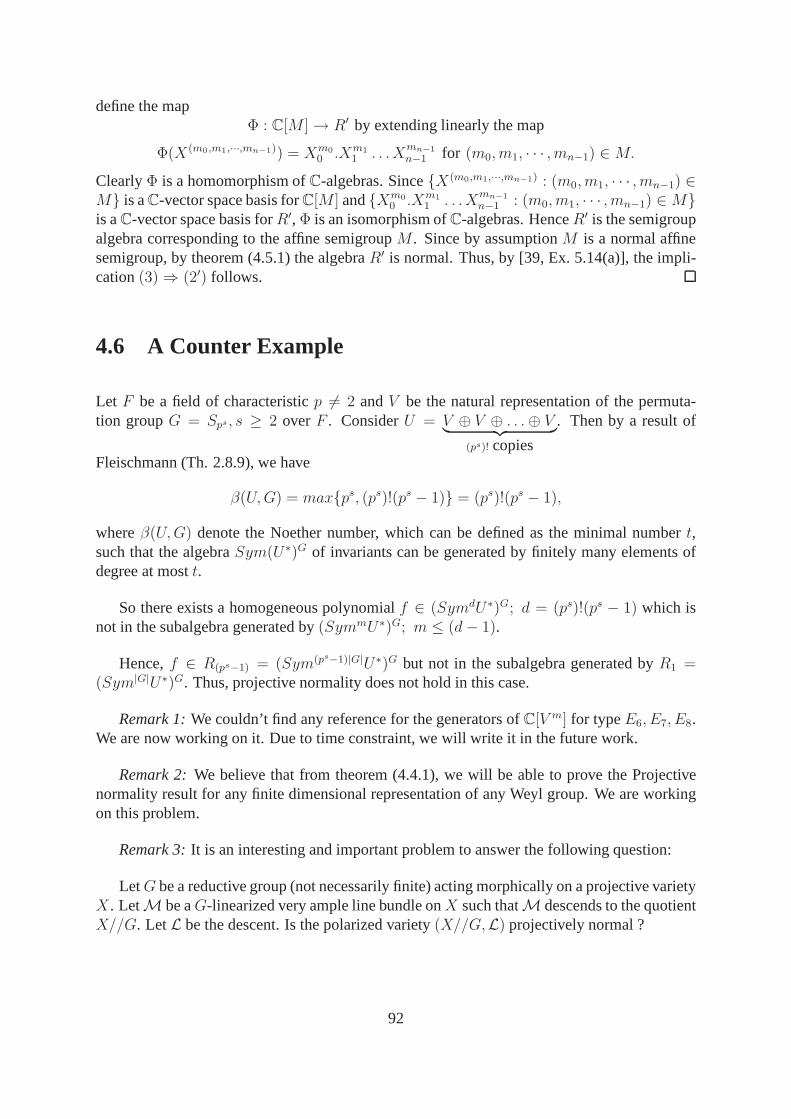
define the mapΦ : C[M ] → R′ by extending linearly the map

Φ(X(m0,m1,···,mn−1)) = Xm0

0 .Xm1

1 . . .Xmn−1

n−1 for (m0, m1, · · · , mn−1) ∈ M.

ClearlyΦ is a homomorphism ofC-algebras. Since{X(m0,m1,···,mn−1) : (m0, m1, · · · , mn−1) ∈M} is aC-vector space basis forC[M ] and{Xm0

0 .Xm1

1 . . .Xmn−1

n−1 : (m0, m1, · · · , mn−1) ∈ M}is aC-vector space basis forR′, Φ is an isomorphism ofC-algebras. HenceR′ is the semigroupalgebra corresponding to the affine semigroupM . Since by assumptionM is a normal affinesemigroup, by theorem (4.5.1) the algebraR′ is normal. Thus, by [39, Ex. 5.14(a)], the impli-cation(3) ⇒ (2′) follows.

4.6 A Counter Example

Let F be a field of characteristicp 6= 2 andV be the natural representation of the permuta-tion groupG = Sps, s ≥ 2 over F . ConsiderU = V ⊕ V ⊕ . . . ⊕ V

︸ ︷︷ ︸

(ps)! copies

. Then by a result of

Fleischmann (Th. 2.8.9), we have

β(U, G) = max{ps, (ps)!(ps − 1)} = (ps)!(ps − 1),

whereβ(U, G) denote the Noether number, which can be defined as the minimalnumbert,such that the algebraSym(U∗)G of invariants can be generated by finitely many elements ofdegree at mostt.

So there exists a homogeneous polynomialf ∈ (SymdU∗)G; d = (ps)!(ps − 1) which isnot in the subalgebra generated by(SymmU∗)G; m ≤ (d − 1).

Hence,f ∈ R(ps−1) = (Sym(ps−1)|G|U∗)G but not in the subalgebra generated byR1 =(Sym|G|U∗)G. Thus, projective normality does not hold in this case.

Remark 1:We couldn’t find any reference for the generators ofC[V m] for typeE6, E7, E8.We are now working on it. Due to time constraint, we will writeit in the future work.

Remark 2:We believe that from theorem (4.4.1), we will be able to provethe Projectivenormality result for any finite dimensional representationof any Weyl group. We are workingon this problem.

Remark 3:It is an interesting and important problem to answer the following question:

Let G be a reductive group (not necessarily finite) acting morphically on a projective varietyX. LetM be aG-linearized very ample line bundle onX such thatM descends to the quotientX//G. LetL be the descent. Is the polarized variety(X//G,L) projectively normal ?

92

Appendix-A

The C-Program:

1 # inc lude<s t d i o . h>2 # inc lude<s t d l i b . h>3 FILE ∗ f i n , ∗ f o u t ;4 i n t r e c S t a c k [ 2 0 0 ] [ 9 ] , n , f u n cS t ack [ 2 0 0 ] ;5 long cn t =0;6 i n t ad j [ 9 ] [ 9 ] ;7 i n t check [1 6 7 7 7 2 1 6 ] ;8 long long o c t [8 ]={1 ,8 ,64 ,512 ,4096 ,32768 ,262144L,2097152L} ;9 long long hash , hashmax =−1;

10 i n t min =1;11 i n t blkComm ( i n t i , i n t l e v e l )12 {13 i n t l =−1, j = l e v e l −1;14 whi le ( j >=1 && ( ad j [ i ] [ f u n cS t ack [ j ] ] ==0 ) )15 {16 i f ( l < f u n cS t ack [ j ] ) l = f u n cS t ack [ j ] ;17 j−−;18 }19 i f ( l > i ) re turn 1 ;20 e l s e i f ( j >=2 && ( i == fu n cS t ack [ j−1]) && ( i > f u n cS t ack [

j ] ) && ( ad j [ i ] [ f u n cS t ack [ j ] ] ==1 ) ) re turn 1 ;21 e l s e re turn 0 ;22 }23 void DFS( i n t l e v e l )24 {25 i n t f l a g t =0;26 f o r ( i n t z =1; z<=n ; z ++)27 i f ( r e c S t a c k [ l e v e l−1][ z ] >0) f l a g t =1;28 i f ( f l a g t ==0)29 {30 hash =0;31 f o r ( i n t j =1; j <=8; j ++)32 {

93

33 hash =hash +( o c t [ j−1]∗( r e c S t a c k [ l e v e l−1][ j ]+7 ) ) ;

34 }35 i f ( check [ hash ]==0)36 {37 cn t ++;38 check [ hash ]=1 ;39 f o r ( i n t j =1; j <=8; j ++) f p r i n t f ( f ou t , ”%d

” , r e c S t a c k [ l e v e l−1][ j ] ) ;40 f p r i n t f ( f ou t , ”\n” ) ;41 f o r ( i n t k =1; k< l e v e l ; k++) f p r i n t f ( f ou t ,

” s%d ” , f u n cS t ack [ k ] ) ;42 f p r i n t f ( f ou t , ”\n” ) ;43 }44 re turn ;45 }46 i n t f l a g =0;47 f o r ( i n t i =1; i <=n ; i ++)48 {49 i f ( r e c S t a c k [ l e v e l−1][ i ] >0 && ( i != f u n cS t ack [

l e v e l −1]) && ( blkComm ( i , l e v e l ) ==0) && ! (l e v e l >1 && ( i == fu n cS t ack [ l e v e l−2]) && ( i >f u n cS t ack [ l e v e l−1]) ) )

50 {51 i f ( ( i ==5 | | i ==6 | | i ==7) && ( r e c S t a c k

[ l e v e l −1][ i −1] + r e c S t a c k [ l e v e l−1][ i+1] < 2∗ r e c S t a c k [ l e v e l−1][ i ] ) )

52 {53 fu n cS t ack [ l e v e l ]= i ;54 f o r ( i n t j =1; j <=n ; j ++)55 {56 i f ( j != i ) r e c S t a c k [

l e v e l ] [ j ]= r e c S t a c k [l e v e l −1][ j ] ;

57 e l s e r e c S t a c k [ l e v e l ] [ j]= r e c S t a c k [ l e v e l−1][ j −1] + r e c S t a c k [l e v e l −1][ j +1]−r e c S t a c k [ l e v e l−1][ j] ;

58 }59 DFS( l e v e l +1) ;60 f l a g =1;61 }62 e l s e i f ( i ==1 && ( r e c S t a c k [ l e v e l

−1][3] <2∗ r e c S t a c k [ l e v e l−1 ] [ 1 ] ) )

94

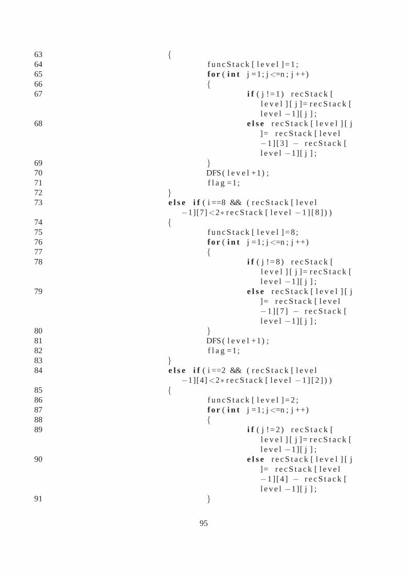
63 {64 fu n cS t ack [ l e v e l ] =1 ;65 f o r ( i n t j =1; j <=n ; j ++)66 {67 i f ( j !=1 ) r e c S t a c k [

l e v e l ] [ j ]= r e c S t a c k [l e v e l −1][ j ] ;

68 e l s e r e c S t a c k [ l e v e l ] [ j]= r e c S t a c k [ l e v e l−1] [3 ] − r e c S t a c k [l e v e l −1][ j ] ;

69 }70 DFS( l e v e l +1) ;71 f l a g =1;72 }73 e l s e i f ( i ==8 && ( r e c S t a c k [ l e v e l

−1][7] <2∗ r e c S t a c k [ l e v e l−1 ] [ 8 ] ) )74 {75 fu n cS t ack [ l e v e l ] =8 ;76 f o r ( i n t j =1; j <=n ; j ++)77 {78 i f ( j !=8 ) r e c S t a c k [

l e v e l ] [ j ]= r e c S t a c k [l e v e l −1][ j ] ;

79 e l s e r e c S t a c k [ l e v e l ] [ j]= r e c S t a c k [ l e v e l−1] [7 ] − r e c S t a c k [l e v e l −1][ j ] ;

80 }81 DFS( l e v e l +1) ;82 f l a g =1;83 }84 e l s e i f ( i ==2 && ( r e c S t a c k [ l e v e l

−1][4] <2∗ r e c S t a c k [ l e v e l−1 ] [ 2 ] ) )85 {86 fu n cS t ack [ l e v e l ] =2 ;87 f o r ( i n t j =1; j <=n ; j ++)88 {89 i f ( j !=2 ) r e c S t a c k [

l e v e l ] [ j ]= r e c S t a c k [l e v e l −1][ j ] ;

90 e l s e r e c S t a c k [ l e v e l ] [ j]= r e c S t a c k [ l e v e l−1] [4 ] − r e c S t a c k [l e v e l −1][ j ] ;

91 }

95

92 DFS( l e v e l +1) ;93 f l a g =1;94 }95 e l s e i f ( i ==4 && ( r e c S t a c k [ l e v e l−1] [3 ]

+ r e c S t a c k [ l e v e l−1] [5 ] + r e c S t a c k [l e v e l −1][2] <2∗ r e c S t a c k [ l e v e l−1 ] [ 4 ] ))

96 {97 fu n cS t ack [ l e v e l ] =4 ;98 f o r ( i n t j =1; j <=n ; j ++)99 {

100 i f ( j !=4 ) r e c S t a c k [l e v e l ] [ j ]= r e c S t a c k [l e v e l −1][ j ] ;

101 e l s e r e c S t a c k [ l e v e l ] [ j]= r e c S t a c k [ l e v e l−1] [3 ] + r e c S t a c k [l e v e l −1] [5 ] +r e c S t a c k [ l e v e l−1][2] − r e c S t a c k [l e v e l −1][ j ] ;

102 }103 DFS( l e v e l +1) ;104 f l a g =1;105 }106 e l s e i f ( i ==3 && ( r e c S t a c k [ l e v e l−1] [1 ]

+ r e c S t a c k [ l e v e l−1][4] <2∗ r e c S t a c k [l e v e l −1 ] [ 3 ] ) )

107 {108 fu n cS t ack [ l e v e l ] =3 ;109 f o r ( i n t j =1; j <=n ; j ++)110 {111 i f ( j !=3 ) r e c S t a c k [

l e v e l ] [ j ]= r e c S t a c k [l e v e l −1][ j ] ;

112 e l s e r e c S t a c k [ l e v e l ] [ j]= r e c S t a c k [ l e v e l−1] [1 ] + r e c S t a c k [l e v e l −1][4]−r e c S t a c k [ l e v e l−1][ j] ;

113 }114 DFS( l e v e l +1) ;115 f l a g =1;116 }117 }

96

118 }119 }120 i n t main ( )121 {122 f i n = fopen ( ” d a t a ” , ” r ” ) ;123 f o u t = fopen ( ” o u t p u t ” , ”w” ) ;124 ad j [ 1 ] [ 3 ] = ad j [ 3 ] [ 1 ] = 1 ;125 ad j [ 2 ] [ 4 ] = ad j [ 4 ] [ 2 ] = 1 ;126 ad j [ 3 ] [ 4 ] = ad j [ 4 ] [ 3 ] = 1 ;127 ad j [ 4 ] [ 5 ] = ad j [ 5 ] [ 4 ] = 1 ;128 ad j [ 6 ] [ 5 ] = ad j [ 5 ] [ 6 ] = 1 ;129 ad j [ 6 ] [ 7 ] = ad j [ 7 ] [ 6 ] = 1 ;130 ad j [ 8 ] [ 7 ] = ad j [ 7 ] [ 8 ] = 1 ;131 whi le ( f s c a n f ( f i n , ”%d” ,&n ) !=EOF){132 i n t i ;133 f o r ( i =1; i <=n ; i ++) f s c a n f ( f i n , ”%d” ,&

r e c S t a c k [ 0 ] [ i ] ) ;134 DFS ( 1 ) ;135 f p r i n t f ( f ou t , ”\n

∗∗∗∗∗∗∗∗∗∗∗∗∗∗∗∗∗∗∗∗∗∗∗∗∗∗∗∗∗∗∗∗∗∗∗∗∗∗∗∗∗\n” ) ;

136 }137 p r i n t f ( ”%d” , cn t ) ;138 f c l o s e ( f i n ) ;139 f c l o s e ( f o u t ) ;140 }

97

Appendix-B

Most of the information given in this appendix are collectedfrom [13] and [45]. For the Weylgroup invariants we refer to [73].

Type An:

Dynkin diagram:

1 2 3 n−1 n:An (n > 1)

Cartan matrix:

1 2 3 . . . n − 1 n

1 2 −12 −1 2 −13 −1 2 .. . . .. . . .. . . .n − 1 . 2 −1n −1 2

Dimension: dim(g) = n(n + 2).

Coxeter number: h = 2|Φ+|n

= n + 1.

Weyl group: W = Sn+1, |W | = (n + 1)!.

Longest element ofW : sn(sn−1sn) · · · (s2 · · · sn)(s1 · · · sn).

The root system:Φ = {ǫi − ǫj : i, j = 1, 2, · · · , n + 1, i 6= j}, where{ǫ1, ǫ2, · · · , ǫn+1} isan orthonormal basis.|Φ| = n(n + 1)

Simple roots: αi = ǫi − ǫi+1, 1 ≤ i ≤ n.

98

Highest long root: α1 + α2 + · · ·+ αn.

Fundamental weights:i = 1n+1

[(n− i + 1)α1 + 2(n− i + 1)α2 + · · ·+ (i− 1)(n− i +1)αi−1 + i(n − i + 1)αi + i(n − i)αi+1 + · · ·+ iαn] i = 1, 2, · · · , n.

Minuscule fundamental weightsEvery fundamental weight is minuscule.

Fundamental group: Zn+1.

Group of diagram automorphisms: Γ = Z2.

Basic polynomial invariants of W: fk =∑n

i=1 xki (1 ≤ k ≤ n).

Type Bn:

Dynkin diagram:

1 2 3 n−1 n( n > :3 )Bn

Cartan matrix:

1 2 3 . . . . n − 2 n − 1 n

1 2 −12 −1 2 −13 −1 2 .. . . .. . . .. . . .n − 2 . 2 −1n − 1 . −1 2 −1n −2 2

Dimension: dim(g) = n(2n + 1).

Coxeter number: h = 2n.

Weyl group: W = (Z2)n ⋊ Sn, |W | = 2nn!.

Longest element ofW : w0 = s1(s2s1)(s3s2s1) · · · (snsn−1 · · · s2s1)(snsn−1 · · · s2)(snsn−1 · · · s3)· · · (snsn−1)sn = −id.

The root system:Φ = Φ1 ∪ Φ2: Φ1 = {±ǫi ± ǫj : i, j = 1, 2, · · · , n, i 6= j}, Φ2 = {±ǫi :i = 1, 2, · · · , n} where{ǫ1, ǫ2, · · · , ǫn} is an orthonormal basis.|Φ| = 2n2.

99

Simple roots: αi = ǫi − ǫi+1, 1 ≤ i ≤ n − 1, αn = ǫn.

Highest long root: α1 + 2α2 + · · ·+ 2αn.

Highest short root: α1 + α2 + · · ·+ αn.

Fundamental weights: i = α1 + 2α2 + · · · + (i − 1)αi−1 + i(αi + αi+1 + · · · + αn)i = 1, 2, · · · , n − 1.

n = 12(α1 + 2α2 + · · · + nαn).

Minuscule fundamental weightsn.

Fundamental group: Z2.

Group of diagram automorphisms: Γ = 1.

Basic polynomial invariants of W: fk =∑n

i=1 x2ki (1 ≤ k ≤ n).

Type Cn:

Dynkin diagram:

1 2 3 n−1 n( n > :3 )Cn

Cartan matrix:

1 2 3 . . . . n − 2 n − 1 n

1 2 −12 −1 2 −13 −1 2 .. . . .. . . .. . . .n − 2 . 2 −1n − 1 . −1 2 −2n −1 2

Dimension: dim(g) = n(2n + 1).

Coxeter number: h = 2n.

Weyl group: W = (Z2)n ⋊ Sn, |W | = 2nn!.

100

Longest element ofW : w0 = s1(s2s1)(s3s2s1) · · · (snsn−1 · · · s2s1)(snsn−1 · · · s2)(snsn−1 · · · s3)· · · (snsn−1)sn = −id.

The root system:Φ = Φ1 ∪Φ2: Φ1 = {±ǫi ± ǫj : i, j = 1, 2, · · · , n, i 6= j}, Φ2 = {±2ǫi :i = 1, 2, · · · , n} where{ǫ1, ǫ2, · · · , ǫn} is an orthonormal basis.|Φ| = 2n2.

Simple roots: αi = ǫi − ǫi+1, 1 ≤ i ≤ n − 1, αn = 2ǫn.

Highest long root: 2α1 + 2α2 + · · ·+ αn.

Highest short root: α1 + 2α2 + · · · + 2αn−1 + αn.

Fundamental weights:i = α1+2α2+· · ·+(i−1)αi−1+i(αi+αi+1+· · ·+αn−1+ 12αn)

i = 1, 2, · · · , n.

Minuscule fundamental weights1.

Fundamental group: Z2.

Group of diagram automorphisms: Γ = 1.

Basic polynomial invariants of W: fk =∑n

i=1 x2ki (1 ≤ k ≤ n).

Type Dn:

Dynkin diagram:

1 2 3 n−3 n−2

n−1

n

Dn (n > 4 ) :

Cartan matrix:

1 2 3 . . . . n − 2 n − 1 n

1 2 −12 −1 2 −13 −1 2 .. . . .. . . .. . . .n − 2 . 2 −1 −1n − 1 . −1 2n −1 2

101

Dimension: dim(g) = n(2n − 1).

Coxeter number: h = 2n − 2.

Weyl group: W = (Z2)n−1 ⋊ Sn, |W | = 2n−1n!.

Longest element ofW : If n is odd:w0 = s1(s2s1)(s3s2s1) · · · (sn−1sn−2 · · · s2s1)(snsn−2 · · · s2s1)(sn−1sn−2 · · · s2)(snsn−2 · · · s3)(sn−1sn−2 · · · s4)(snsn−2 · · · s5) · · · (snsn−2)sn−1.

If n is even:w0 = s1(s2s1)(s3s2s1) · · · (sn−1sn−2 · · · s2s1)(snsn−2 · · · s2s1)(sn−1sn−2 · · · s2)(snsn−2 · · · s3)(sn−1sn−2 · · · s4)(snsn−2 · · · s5) · · · (sn−1sn−2)sn = −id.

The root system:Φ = {±ǫi ± ǫj : i, j = 1, 2, · · · , n, i 6= j}, where{ǫ1, ǫ2, · · · , ǫn} is anorthonormal basis.|Φ| = 2n(n − 1).

Simple roots: αi = ǫi − ǫi+1, 1 ≤ i ≤ n − 1, αn = ǫn−1 + ǫn.

Highest long root: α1 + 2α2 + · · ·+ 2αn−2 + αn−1 + αn.

Fundamental weights:i = α1 + 2α2 + · · ·+ (i− 1)αi−1 + i(αi + αi+1 + · · ·+ αn−2) +12i(αn−1 + αn) i = 1, 2, · · · , n − 2.

n−1 = 12(α1 + 2α2 + · · · + (n − 2)αn−2 + 1

2nαn−1 + 1

2(n − 2)αn).

n = 12(α1 + 2α2 + · · · + (n − 2)αn−2 + 1

2(n − 2)αn−1 + 1

2nαn).

Minuscule fundamental weights1, n−1, n.

Fundamental group: Z4 if l is odd andZ2 × Z2 if n is even.

Group of diagram automorphisms: Γ =

{S3 if n = 4;Z2 if n > 4.

Basic polynomial invariants of W: fk =∑n

i=1 x2ki (1 ≤ k ≤ n−1) andfn = x1x2 . . . xn.

Type E6:

Dynkin diagram:

1:

6543

2

6E

Cartan matrix:

102

1 2 3 4 5 6

1 2 −1 0 0 0 02 −1 2 −1 0 0 03 0 −1 2 −1 −1 04 0 0 −1 2 0 05 0 0 −1 0 2 −16 0 0 0 0 −1 2

Dimension: dim(g) = 78.

Coxeter number: h = 12.

Order of the Weyl group: |W | = 27345.

Longest element ofW : w0 = s1(s2s3s1)(s4s2s3s1)(s4s3)(s5s4s2s3s1)(s4s3)(s5s4s2)(s6s5s4s2s3s1)(s4s3)(s5s4s2)(s6s5s4s3s1).

The root system: Φ = {±ǫi ± ǫj : i, j = 1, 2, · · · , 5, i 6= j} ∪ {12

∑8i=1 ciǫi : ci =

±1,∏8

i=1 ci = 1, c6 = c7 = c8}, where{ǫ1, ǫ2, · · · , ǫ8} is an orthonormal basis ofR8. |Φ| =72.

Simple roots: αi = ǫi − ǫi+1, 1 ≤ i ≤ 4, α5 = ǫ4 + ǫ5, α6 = −12(ǫ1 + ǫ2 + · · ·+ ǫ8).

Highest long root: α1 + 2α2 + 2α3 + 3α4 + 2α5 + α6.

Fundamental weights:1 = 13(4α1 + 3α2 + 5α3 + 6α4 + 4α5 + 2α6).

2 = α1 + 2α2 + 2α3 + 3α4 + 2α5 + α6.

3 = 13(5α1 + 6α2 + 10α3 + 12α4 + 8α5 + 4α6).

4 = 2α1 + 3α2 + 4α3 + 6α4 + 4α5 + 2α6.

5 = 13(4α1 + 6α2 + 8α3 + 12α4 + 10α5 + 5α6).

6 = 13(2α1 + 3α2 + 4α3 + 6α4 + 5α5 + 4α6).

Minuscule fundamental weights:1, 6.

Fundamental group: Z3.

Group of diagram automorphisms: Z2.

Basic polynomial invariants of W: fm =∑6

i=1(yi+y)m+∑6

i=1(yi−y)m−∑

i<j(yi+yj)m,

m = 2, 5, 6, 8, 9, 12, wherey1 = 5x1+4x2+3x3+2x4+x5, y2 = −x1+4x2+3x3+2x4+x5, y3 = −x1−2x2+3x3+2x4+x5,

103

y4 = −x1 − 2x2 − 3x3 + 2x4 + x5, y5 = −x1 − 2x2 − 3x3 − 42x4 + x5, y6 = −∑5

i=1 yi andy = −3(x1 + 2x2 + 3x3 + 2x4 + x5 + 2x6).

Type E7:

Dynkin diagram:

1:

6543

2

E7

7

Cartan matrix:

1 2 3 4 5 6 7

1 2 −1 0 0 0 0 02 −1 2 −1 0 0 0 03 0 −1 2 −1 0 0 04 0 0 −1 2 −1 −1 05 0 0 0 −1 2 0 06 0 0 0 −1 0 2 −17 0 0 0 0 0 −1 2

Dimension: dim(g) = 133.

Coxeter number: h = 18.

Order of the Weyl group: |W | = 210.34.5.7.

Longest element ofW : w0 = s1(s2s3s1)(s4s2s3s1)(s4s3)(s5s4s2s3s1)(s4s3)(s5s4s2)(s6s5s4s2s3s1)(s4s3)(s5s4s2)(s6s5s4s3s1)(s7s6s5s4s2s3s1)(s4s3)(s5s4s2)(s6s5s4s3s1)(s7s6s5s4s2)(s3s4s5s6s7) = −id.

The root system:Φ = {±ǫi±ǫj : i, j = 1, 2, · · · , 6, i 6= j}∪{±(ǫ7+ǫ8)}∪{12

∑8i=1 ciǫi :

ci = ±1,∏8

i=1 ci = 1, c7 = c8}, where{ǫ1, ǫ2, · · · , ǫ8} is an orthonormal basis ofR8. |Φ| =126.

Simple roots: αi = ǫi − ǫi+1, 1 ≤ i ≤ 5, α6 = ǫ5 + ǫ6, α7 = −12(ǫ1 + ǫ2 + · · ·+ ǫ8).

Highest long root: 2α1 + 2α2 + 3α3 + 4α4 + 3α5 + 2α6 + α7.

Fundamental weights:1 = 2α1 + 2α2 + 3α3 + 4α4 + 3α5 + 2α6 + α7.

104

2 = 12(4α1 + 7α2 + 8α3 + 12α4 + 9α5 + 6α6 + 3α7).

3 = 3α1 + 4α2 + 6α3 + 8α4 + 6α5 + 4α6 + 2α7.

4 = 4α1 + 6α2 + 8α3 + 12α4 + 9α5 + 6α6 + 3α7.

5 = 12(6α1 + 9α2 + 12α3 + 18α4 + 15α5 + 10α6 + 5α7).

6 = 2α1 + 3α2 + 4α3 + 6α4 + 5α5 + 4α6 + 2α7.

7 = 12(2α1 + 3α2 + 4α3 + 6α4 + 5α5 + 4α6 + 3α7).

Minuscule fundamental weights:7.

Fundamental group: Z2.

Group of diagram automorphisms: 1.

Basic polynomial invariants of W: fm =∑

i<j(yi + yj)m, i, j ∈ {1, 2, · · · , 8}, m =

2, 6, 8, 10, 12, 14, 18, wherey1 = 3x1 + 2x2 + x3 − x7, y2 = −x1 + 2x2 + x3 − x7, y3 =−x1 − 2x2 + x3 − x7, y4 = −x1 − 2x2 − 3x3 − x7, y5 = −x1 − 2x2 − 3x3 − 4x4 − x7,y6 = −x1 − 2x2 − 3x3 − 4x4 − 4x5 − x7, y7 = −x1 − 2x2 − 3x3 − 4x4 − 4x5 − 4x6 − x7,y8 = −

∑7i=1 yi.

Type E8:

Dynkin diagram:

1 6543

2

E7 8

:8

Cartan matrix:

1 2 3 4 5 6 7 8

1 2 −1 0 0 0 0 0 02 −1 2 −1 0 0 0 0 03 0 −1 2 −1 0 0 0 04 0 0 −1 2 −1 0 0 05 0 0 0 −1 2 −1 −1 06 0 0 0 0 −1 2 0 07 0 0 0 0 −1 0 2 −18 0 0 0 0 0 0 −1 2

105

Dimension: dim(g) = 248.

Coxeter number: h = 30.

Order of the Weyl group: |W | = 214.35.52.7.

Longest element ofW : w0 = s1(s2s3s1)(s4s2s3s1)(s4s3)(s5s4s2s3s1)(s4s3)(s5s4s2)(s6s5s4s2s3s1)(s4s3)(s5s4s2)(s6s5s4s3s1)(s7s6s5s4s2s3s1)(s4s3)(s5s4s2)(s6s5s4s3s1)(s7s6s5s4)(s2s3s4s5s6s7)(s8s7s6s5s4s2s3s1)(s4s3)(s5s4s2)(s6s5s4s3s1)(s7s6s5s4s2)(s3s4s5s6s7)(s8s7s6s5s4s2s3s1)(s4s3)(s5s4s2)(s6s5s4s3s1)(s7s6s5s4s2)(s3s4s5s6s7s8) = −id.

The root system: Φ = {±ǫi ± ǫj : i, j = 1, 2, · · · , 8, i 6= j} ∪ {12

∑8i=1 ciǫi : ci =

±1,∏8

i=1 ci = 1}, where{ǫ1, ǫ2, · · · , ǫ8} is an orthonormal basis ofR8. |Φ| = 240.

Simple roots: αi = ǫi − ǫi+1, 1 ≤ i ≤ 6, α7 = ǫ6 + ǫ7, α7 = −12(ǫ1 + ǫ2 + · · ·+ ǫ8).

Highest long root: 2α1 + 3α2 + 4α3 + 6α4 + 5α5 + 4α6 + 3α7 + 2α8.

Fundamental weights:1 = 4α1 + 5α2 + 7α3 + 10α4 + 8α5 + 6α6 + 4α7 + 2α8.

2 = 5α1 + 8α2 + 10α3 + 15α4 + 12α5 + 9α6 + 6α7 + 3α8.

3 = 7α1 + 10α2 + 14α3 + 20α4 + 16α5 + 12α6 + 8α7 + 4α8.

4 = 10α1 + 15α2 + 20α3 + 30α4 + 24α5 + 18α6 + 12α7 + 6α8.

5 = 8α1 + 12α2 + 16α3 + 24α4 + 20α5 + 15α6 + 10α7 + 5α8.

6 = 6α1 + 9α2 + 12α3 + 18α4 + 15α5 + 12α6 + 8α7 + 4α8.

7 = 4α1 + 6α2 + 8α3 + 12α4 + 10α5 + 8α6 + 6α7 + 3α8.

8 = 2α1 + 3α2 + 4α3 + 6α4 + 5α5 + 4α6 + 3α7 + 2α8.

Minuscule fundamental weights:No miniscule fundamental weights.

Fundamental group: 1.

Group of diagram automorphisms: 1.

Basic polynomial invariants of W: fm = 2∑

i<j[(yi+yj)m+(yi−yj)

m]+∑

Q

ǫi=−1,ǫi=±1

(∑

ǫixi)m, i, j ∈ {1, 2, · · · , 8}, m = 2, 8, 12, 14, 18, 20, 24, 30, wherey1 = 2x1 + 2x2 + 2x3 +

2x4 + 2x5 + x6 + x8, y2 = 2x2 + 2x3 + 2x4 + 2x5 + x6 + x8, y3 = 2x3 + 2x4 + 2x5 + x6 + x8,y4 = 2x4 + 2x5 + x6 + x8, y5 = 2x5 + x6 + x8, y6 = x6 + x8, y7 = x6 + x8, y8 =2x1 + 4x2 + 6x3 + 8x4 + 10x5 + 7x6 + 4x7 + 5x8.

Type F4:

106

Dynkin diagram:

1 2 3 4:F4

Cartan matrix:

1 2 3 4

1 2 −1 0 02 −1 2 −1 03 0 −2 2 −14 0 0 −1 2

Dimension: dim(g) = 52.

Coxeter number: h = 12.

Weyl group: W = (Z32 ⋊ S4) ⋊ S3, |W | = 27.32.

Longest element ofW : w0 = s1s2s1s3s2s1s3s2s3s4s3s2s1s3s2s3s4s3s2s1s3s2s3s4 = −id.

The root system: Φ = {±ǫi ± ǫj : i, j = 1, 2, 3, 4, i 6= j} ∪ {±ǫi : i = 1, 2, 3, 4} ∪{1

2

∑4i=1 ciǫi : ci = ±1,

∏4i=1 ci = 1}, where{ǫ1, ǫ2, ǫ3, ǫ4} is an orthonormal basis.|Φ| = 48.

Simple roots: α1 = ǫ1 − ǫ2, α2 = ǫ2 − ǫ3 α3 = ǫ3, α4 = −frac12(−ǫ1 − ǫ2 − ǫ3 + ǫ4).

Highest long root: 2α1 + 3α2 + 4α3 + 2α4.

Highest short root: α1 + 2α2 + 3α3 + 2α4.

Fundamental weights:1 = 2α1 + 3α2 + 4α3 + 2α4.

2 = 3α1 + 6α2 + 8α3 + 4α4.

3 = 2α1 + 4α2 + 6α3 + 3α4.

4 = α1 + 2α2 + 3α3 + 2α4.

Minuscule fundamental weights:No miniscule fundamental weights.

Fundamental group: 1.

Group of diagram automorphisms: 1.

Basic polynomial invariants of W: f2k =∑

1≤i≤j≤4((xi + xj)2k + (xi − xj)

2k), k =1, 3, 4, 6.

Type G2:

107

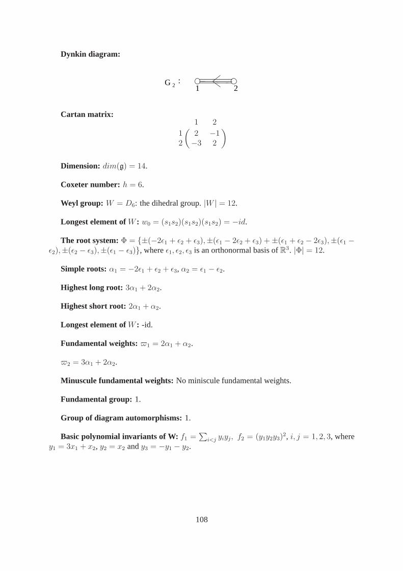
Dynkin diagram:

21G 2

:

Cartan matrix:

(1 2

1 2 −12 −3 2

)

Dimension: dim(g) = 14.

Coxeter number: h = 6.

Weyl group: W = D6: the dihedral group.|W | = 12.

Longest element ofW : w0 = (s1s2)(s1s2)(s1s2) = −id.

The root system:Φ = {±(−2ǫ1 + ǫ2 + ǫ3),±(ǫ1 − 2ǫ2 + ǫ3) + ±(ǫ1 + ǫ2 − 2ǫ3),±(ǫ1 −ǫ2),±(ǫ2 − ǫ3),±(ǫ1 − ǫ3)}, whereǫ1, ǫ2, ǫ3 is an orthonormal basis ofR3. |Φ| = 12.

Simple roots: α1 = −2ǫ1 + ǫ2 + ǫ3, α2 = ǫ1 − ǫ2.

Highest long root: 3α1 + 2α2.

Highest short root: 2α1 + α2.

Longest element ofW : -id.

Fundamental weights:1 = 2α1 + α2.

2 = 3α1 + 2α2.

Minuscule fundamental weights:No miniscule fundamental weights.

Fundamental group: 1.

Group of diagram automorphisms: 1.

Basic polynomial invariants of W: f1 =∑

i<j yiyj, f2 = (y1y2y3)2, i, j = 1, 2, 3, where

y1 = 3x1 + x2, y2 = x2 andy3 = −y1 − y2.

108

Bibliography

[1] O. M. Adamovich, E. O. Golovina,Simple Linear Lie Groups having a Free algebra ofInvarisnts, Questions of Group Theory and Homological Algebra Vyp 2, Yaroslav. Gros.Unir. Yaroslavl’ 3-41 (1980) English Translation in Sel. Math. Sov. 3, 183-220 (1983/84).

[2] A. Borel, Linear algebraic groups, Second edition, Graduate Texts in Mathematics, 126.Springer Verlag, New York, 1991.

[3] N. Bourbaki, Lie groups and Lie algebras, Chapters 4-6, Elements of Mathematics(Berlin), Springer-Verlag, 2002.

[4] A. Broer, Remarks on invariant theory of finite groups, preprint, Universite de Montreal,Montreal, 1997.

[5] A. Broer, On Chevalley-Shephard-Todd’s theorem in positive characteristic, Symmetryand spaces, 21-34, Progr. Math., 278, Birkhauser Boston, Inc., Boston, MA, 2010.

[6] W. Bruns, J. Gubeladze,Polytopes, Rings, and K-Theory, Springer Monographs in Math-ematics. Springer, Dordrecht, 2009.

[7] R. Bryant, G. Kemper,Global degree bounds and the transfer principle for invariants, J.Algebra 284 (2005), no. 1, 80-90.

[8] H. E. A. Campbell, A. V. Geramita, I. P. Hughes, J. R. Shank, D. L. Wehlau,Non-Cohen-Macaulay vector invariants and a Noether bound for a Gorenstein ring of invariants,Canad. Math. Bull. 42 (1999), no. 2, 155-161.

[9] H. E. A. Campbell, I. P. Hughes, G. Kemper, R. J. Shank and D. L. Wehlau,Depth ofmodular invariant rings, Transformation Groups5 (2000) no. 1, 21-34.

[10] H. E. A. Campbell, D. L. Wehlau,Modular Invariant Theory, Encyclopaedia of Math-ematical Sciences, 2011, Volume 139, Invariant Theory and Algebraic TransformationGroups, Springer-Verlag.

[11] E. Cartan,”Les tenseurs irreductibles et les groupes lineaires simples et semi-simples”Bull. Sci. Math., 49 (1925) pp. 130-152.

[12] R. W. Carter,Finite Groups of Lie type, John Wiley, New York, 1993.

[13] R. W. Carter,Lie Algebras of Finite and Affine Type, Cambridge studies in advancedmathematics 96 (2005).

109

[14] C. Chevalley,Theorie des groupes de Lie. II, Hermann, Paris, 1951.

[15] C. Chevalley,Invariants of Finite Groups Generated by Reflections, Amer. J. Math.77(1955), 778-782.

[16] C. Chevalley,Classification des groupes algebriques semi-simples, Springer-Verlag,Berlin, 2005. Collected works. Vol. 3, Edited and with a preface by P. Cartier, With thecollaboration of Cartier, A. Grothendieck and M. Lazard.

[17] H. Chu, S. J. Hu, M. C. Kang,A note on Projective normality, Proc. Amer. Math. Soc.139 (2011), no. 8, pp. 863-867.

[18] D. Daigle, G. Freudenburg,A counter example to Hilbert’s fourteenth problem in dimen-sion 5. J. Algebra, 221(2), 528-535, 1999.

[19] M. Demazure,Une demonstration algebrique d’un theoreme de Bott(French), Invent.Math. 5 (1968) 349-356.

[20] M. Demazure,A very simple proof of Bott’s theorem, Invent. Math. 33 (1976), no. 3,271-272.

[21] H. Derksen,Computation of invariants for reductive groups, Adv. Math. 141, no. 2, 366-384. 1998.

[22] H. Derksen, G. Kemper,Computational Invariant Theory, Encyclopaedia of Mathemati-cal Sciences 130, Springer-Verlag, Berlin, Heidelberg, New York 2002.

[23] L. E. Dickson,Binary Modular Groups and their Invariants, Amer. J. of Math. 33 (1911),175-192.

[24] I. V. Dolgachev and Y. Hu,Variation of geometric invariant theory quotients, Inst. HautesAtudes Sci. Publ. Math. (1998), no. 87, 5-56.

[25] I. V. Dolgachev,Lectures on invariant theory, London Mathematical Society Lecture NoteSeries, 296.Cambridge University Press, Cambridge, 2003.

[26] M. Domokos, P. Hegedus,Noether’s bound for polynomial invariants of finite groups,Arch. Math. (Basel) 74 (2000), no. 3, 161-167.

[27] M. Domokos,Vector invariants of a class of pseudo-reflection groups andmultisymmetricsyzygies, J. Lie Theory 19 (2009), no. 3, 507-525.

[28] A. Dress,On Finite Groups Generated by Pseudo-refiections, J. of Algebra 11 (1969),1-5.

[29] J. M. Drezet, M.S. Narasimhan,Groupe de Picard des varieties de modules de fibrerssemi-stables sur les courbes algebriques, Invent. Math. 97, 53-94 (1989)

[30] G. Ellingsrud and T. Skjelbred,Profondeur d’Anneaux d’Invariants en Caracteristique p,Compos. Math.. 41, (1980), pp 233-244.

110

[31] P. Erdos, A. Ginzburg, A. Ziv,A theorem in additive number theory, Bull. Res. Council,Israel, 10 F(1961) 41-43.

[32] P. Fleischmann,A new degree bound for the vector invariants of symmetric groups, Trans.Amer. Math. Soc. 350 (1998), 1703-1712.

[33] P. Fleischmann,The Noether bound in invariant theory of finite groups, Adv. Math. 152(2000), pp. 23-32.

[34] P. Fleischmann, G. Kemper and R.J. Shank,Depth and Cohomological Connectivityin Modular Invariant Theory, Transactions of the American Mathematical Society 357(2005) no. 9, 3605-3621.

[35] P. Fleischmann, M. Sezer, R. J. Shank, C. F. Woodcock,The Noether numbers for cyclicgroups of prime order, Adv. Math. 207 (2006), no. 1, 149-155.

[36] P. Fleischmann, C. F. Woodcock,Non-linear Group Actions with Polynomial InvariantRings and a Structure Theorem for Modular Galois Extensions, arXiv:1011.5149v1.

[37] J. Fogarty,On Noether’s bound for polynomial invariants of a finite group, Electron. Res.Announc. Amer. Math. Soc., 7, 5-7, 2001.

[38] R. Goodman, N. Wallach,Symmetry, Representations, and Invariants, Springer, 2009.

[39] R. Hartshorne,Algebraic Geometry, Graduate Texts in Math., 52, Springer-Verlag, NewYork-Heidelberg, 197.

[40] D. Hilbert,Uber die Theorie der algebraischen Formen, Mathematische Annalen 36, 473-534.

[41] M. Hochster and J. A. Eagon,Cohen-Macaulay Rings, Invariant Theory, and the GenericPerfection of Determinantal Loci, Amer. J. of Math. 93 (1971), 1020-1058.

[42] M. Hochster, J. Roberts,Rings of invariants of reductive groups acting on regular ringsare Cohen Macaulay, Adv.Math. 13 (1974) 115-175.

[43] M. Hochster and C. Huneke,Tight closure, invariant theory, and the Briancon-Skodatheorem. J. Amer. Math. Soc. 3 (1990), pp. 31-116.

[44] J. E. Humphreys,Modular representations of classical Lie algebras and semi-simplegroups, J. Algebra 19 (1971), 51-79.

[45] J. E. Humphreys,Introduction to Lie algebras and representation theory, Springer, BerlinHeidelberg, 1972.

[46] J. E. Humphreys,Linear Algebraic Groups, Springer-Verlag, 1975.

[47] J. E. Humphreys,Reflection Groups and Coxeter Groups, Cambridge studies in advancedmathematics, 29 (1990).

[48] M. Hunziker,Classical invariant theory for finite reflection groups, Transform. Groups 2(1997) (2), pp. 147-163.

111

[49] J. C. Jantzen,Representations of Algebraic Groups, Academic Press, New York (1987).

[50] V. G. Kac, V.L. Popov, E.B. Vinberg,Sur les groupes lineages algebriques dont l’agebredes invaxiantes est libre, C.R. Acad. Sci. Paris Ser. I Math. 283. 865-878 (1976).

[51] R. Kane,Reflection Groups and Invariant theory, CMS Books in Mathematics, Springer-Verlag, 2001.

[52] S. S. Kannan,Torus quotients of homogeneous spaces, Proc. Indian Acad. Sci.(Math. Sci),108(1998), no 1, 1-12.

[53] S. S. Kannan,Torus quotients of homogeneous spaces-II, Proc. Indian Acad. Sci.(Math.Sci), 109(1999), no 1, 23-39.

[54] S. S. Kannan,Cohomology of line bundles on Schubert varieties in the Kac-Moody setting,J. Algebra, 310(2007) 88-107.

[55] S. S. Kannan, S.K. Pattanayak, Pranab Sardar,Projective normality of finite groups quo-tients, Proc. Amer. Math. Soc. 137 (2009), no. 3, pp. 863-867.

[56] S. S. Kannan, Pranab Sardar,Torus quotients of homogeneous spaces of the general lineargroup and the standard representation of certain symmetricgroups, Proc. Indian Acad.Sci.(Math. Sci), 119(2009), no 1, 81-100.

[57] S. S. Kannan, S.K. Pattanayak,Torus quotients of homogeneous spaces - minimal dimen-sional Schubert varieties admitting semi-stable points, Proc. Indian Acad. Sci.(Math. Sci),119(2009), no 4, 469-485.

[58] S. S. Kannan, S.K.Pattanayak,Projective normality of Weyl group quotients, Proc. IndianAcad. Sci.(Math. Sci), 121 (2011), no.1, pp. 1-8.

[59] S. S. Kannan, S.K. Pattanayak,Normality, Projective normality and EGZ theorem, willappear in Integers.

[60] G. Kemper,Calculating invariant rings of finite groups over arbitraryfields, J. SymbolicComput. 21 (1996), 351-366.

[61] G. Kemper and G. Malle,The finite irreducible linear groups with polynomial ring ofinvariants, Transform. Groups 2 (1997), no. 1, 57-89.

[62] G. Kemper,Lower degree bounds for modular invariants and a question ofI. Hughes,Transform. Groups 3 (1998), no. 2, 135-144.

[63] G. Kemper,On the Cohen Macaulay property of modular invariant rings, J. Algebra 215(1999) 330-351.

[64] G. Kemper,Die Cohen-Macaulay-Eigenschaft in der modularen Invariantentheorie. Ha-bilitationsschrift, Universitat Heidelberg, 1999.

[65] G. Kemper,A characterization of linearly reductive groups by their invariants, Transform.Groups 5 (1) (2000) 85-92.

112

[66] G. Kemper,The depth of invariant rings and cohomology, with an appendix by K. Maga-ard. J. Algebra. 245 no. 2, 463-531 (2001).

[67] F. Knop,Der kanonische Modul eines Invariantenrings, J. Algebra 127 (1989), pp. 40-54.

[68] M. Kohls, On the depth of invariant rings of infinite groups, J. Algebra 322 (2009), 210-218.

[69] H. Kraft, P. Slodowy, T. A. Springer,Algebraic Transformation Groups and InvariantTheory, Birkhauser, 1989.

[70] H. P. Kraft and C. Procesi,Classical invariant theory: A primerlecture notes (1996),http://www.math.unibas.ch/ kraft/Papers/KP-Primer.pdf.

[71] D. Krause,Die Noethersche Gradgrenze in der Invariantentheorie, Diplomarbeit, Univer-sity of G ttingen, 1999.

[72] V. Lakshmibai and K. N. Raghavan,Standard Monomial Theory, Encyclopaedia of Math-ematical Sciences, vol. 137, Springer, 2008.

[73] C. Y. Lee,Invariant polynomials of Weyl groups and applications to the centers of univer-sal enveloping algebras, Can. J. Math., XXVI (1974), 583-592.

[74] P. Littelmann,Koregulare und aqnidimensionale Darstellungen. J. Algebra 123, No. 1193-222 (1989).

[75] Y. Matsushima,Espaces homogenes de Stein des groupes de Lie complexes, Nagoya Math.J. 16 (1960), 205-218.

[76] M. L. Mehta,Basic set of invariant polynomials for finite reflection groups, Com. in Alg.,16. (5), (1988), 1083-1098.

[77] T. Molien, Uber die Invarianten der linearen Substitutionsgruppen, Sitzungsber. Konig.Preuss. Akad. Wiss. (1897), 1152-1156.

[78] D. Mumford, J. Fogarty and F. Kirwan,Geometric Invariant theory, Springer-Verlag,1994.

[79] M. Nagata,On the 14th problem of Hilbert, Amer. J. Math., 8l (1959), 766-772.

[80] M. Nagata,Complete reducibility of rational representations of a matric group, J. Math.Kyoto Univ. 1 (1961) 87-99.

[81] M. Nagata,”Invariants of a group in an affine ring”, J. Math. Kyoto Univ., 3 (1964) pp.369-377.

[82] H. Nakajima, Invariants of Finite Groups Generated by Pseudoreflectionsin PositiveCharacteristic, Tsukuba J. of Math. 3 (1979), 109-122.

[83] H. Nakajima,Relative invariants of finite groups, J. Algebra, 79 (1982) 218-234.

113

[84] H. Nakajima,Modular Representations of Abelian Groups with Regular Rings of Invari-ants, Nagoya Math. J. 86 (1982), 229-248.

[85] H. Nakajima,Regular rings of invariants of unipotent groups, J. Algebra 85 (1983), pp.253-286.

[86] M. D. Neusel and L. Smith,Invariant Theory of Finite Groups, Math. Surveys and. Mono-graphs Vol. 94, AMS, Providence RI 2002.

[87] P. E. Newstead,Introduction to Moduli Problems and Orbit Spaces, TIFR Lecture Notes,1978.

[88] E. Noether,Der Endlichkeitssatz der Invarianten endlicher Gruppen, Math. Ann. 77,(1916), 89-92.

[89] E. Noether,Der Endlichkeitssatz der Invarianten endlich linearer Gruppen der Charak-teristik p, Nachr. Akad. Wiss. Gottingen (1926), 28-35.

[90] V. L. Popov,On Hilbert’s theorem on invariants(in Russian), Dokl. Akad. Nauk SSSR249 (1979), 551–555.; English translation in Soviet Math. Dokl. 20 (1979), 1318-1322.

[91] V. Popov,Constructive invariant theory, Asterisque, 87-88 (1981), 303-334.

[92] V. L. Popov,The Constructive Theory of Invariants, Math. USSR Izvest. 10 (1982), 359-376.

[93] D. R. Richman,Invariants of finite groups over fields of characteristic p. Adv. Math. 124(1996), no. 1, 25-48.

[94] P. Roberts,An infinitely generated symbolic blow-up and a new counterexample toHilbert’s fourteenth problem, J. of Algebra 132, pp. 461-473 (1990).

[95] D. J. S. Robinson,A Course in the Theory of Groups, 2nd ed., Springer-Verlag, 1996.

[96] B. J. Schmid,Finite groups and invariant theory, Topics in invariant theory (Paris, 1989-1990), pp. 35-66, Lecture Notes in Math. 1478, Springer, 1991.

[97] G. W. Schwarz,Representations of Simple Lie Groups with Regular Rings on Invariants,Inv. Math. 49 167-191 (1978).

[98] J. P. Serre,Groupes finis d’automorphisms d’anneaux locaux reguliers, Colloq. d’Alg.Ecole Norm. de Jeunes Filles, Paris (1967), 1-11.

[99] J. P. Serre,Linear representations of finite groups, Graduate Texts in Mathematics, vol.42, Springer-Verlag, New York, Heidelberg, Berlin, 1977.

[100] C. S. Seshadri,Mumford’s conjecture for GL (2) and applications, International Collo-quim on Algebraic Geometry, Bombay, 16-23 January (1968).

[101] C. S. Seshadri,Quotient spaces modulo reductive algebraic groups, Ann. Math.95(1972) 511-556.

114

[102] C. S.Seshadri, Introduction to the theory of standard monomials, Brandeis LectureNotes 4, June 1985.

[103] M. Sezer,Sharpening the generalized Noether bound in the invariant theory of finitegroups, J. Algebra 254 (2002) 252-263.

[104] R. J. Shank,S.A.G.B.I. bases for rings of formal modular seminvariants, CommentariiMathematici Helvetici 73 (1998) no. 4, 548-565.

[105] R. J. Shank and D.L. Wehlau,Computing modular invariants of p-groups, Journal ofSymbolic Computation 34 (2002) no. 5, 307-327.

[106] G. C. Shephard, J.A.Todd,Finite Unitary Reflection Groups, Canadian J. Math. 6,(1954), 274-304.

[107] A. N. Skorobogatov,Automorphisms and forms of torus quotients of homogeneousspaces, (Russian) Mat. Sb. 200 (2009), no. 10, 107-122.

[108] L. Smith and R. E. Stong,Invariants of Finite Groups, unpublished correspondence,1979-1993.

[109] L. Smith,Polynomial invariants of finite groups, A. K. Peters, Wellesley, Mass. 1995.

[110] L. Smith,E. Noether’s bound in the invariant theory of finite groups, Arch. Math.(Basel)66 (1996), no. 2, 89-92.

[111] L. Smith,Putting the squeeze on the Noether gap-the case of the alternating groupsAn,Math. Ann. 315 (1999), no. 3, 503-510.

[112] L. Smith,Noether’s bound in the invariant theory of finite groups and vector invariantsof iterated wreath products of symmetric groups, Quartely. J. Math. 51 (2000), no. 1,93-105.

[113] D. M. Snow,The nef value and defect of homogeneous line bundles, Trans. Amer. Math.Soc. 340 1 (1993), pp. 227-241.

[114] T. A. Springer,Invariant theory, Lecture Notes in Math., vol. 585, Springer-Verlag,Berlin and New York, 1977.

[115] T. A. Springer,Linear algebraic groups, Progress in Mathematics, vol. 9, Birkhauser,Boston; Basel, Stuttgart, 1981, 304 pp.

[116] E. Strickland,Quotients of flag varieties by a maximal torus. Math. Z. 234(2000, no.1,1-7; translation in Sb. Math. 200 (2009), no. 9-10, 1521-1536.

[117] P. Symonds,On the Castelnuovo-Mumford regularity of rings of polynomial invariants,preprint, available at http://www.maths.manchester.ac.uk/ pas/preprints/ (2009).

[118] P. Tauvel, R. W. T. Yu,Lie algebras and algebraic groups, Springer Monographs inMathematics, Springer Verlag, Berlin, 2005.

115

[119] N. R. Wallach,Invariant differential operators on a reductive Lie algebra and Weyl grouprepresentations, J. Amer. Math. Soc. 6 (1993) (4), pp. 779-816.

[120] D. Wehlau,Constructive invariant theory for tori, Ann. Inst. Fourier, Grenoble 43(1993), pp. 1055-1066.

[121] D. Wehlau,When is a ring of torus invariants a polynomial ring, Manuscripta Math. 82,161-170 (1994).

[122] R. Weitzenbock,Uber die Invarianten von Linearen Gruppen, Acta Math., 58 (1932), p.231-293.

[123] H. Weyl,The Classical Groups. Their Invariants and Representations, Princeton Univ.Press (1946).

[124] Y. Wu, Invariants of Modular Two-Row Groups, Ph.D thesis, Queen’s University, 2009.

[125] O. Zariski,Interpretations algebrico-geometrique de quatorzieme probleme de Hilbert,Bull. Sci. Math. 78 (1954), 155-168.

[126] V. S. Zhgun,Variation of the Mumford quotient for torus actions on complete flag mani-folds. I, (Russian) Izv. Ross. Akad. Nauk Ser. Mat. 71 (2007), no. 6, 29-46; translation inIzv. Math. 71 (2007), no. 6, 1105-1122.

[127] V. S. Zhgun,Variation of the Mumford quotient for torus actions on complete flag mani-folds. II, (Russian) Mat. Sb. 199 (2008), no. 3, 25-44; translation inSb. Math. 199 (2008),no. 3-4, 341-359.

Chennai Mathematical InstitutePlot No-H1, SIPCOT IT ParkPadur Post, SiruseriTamilnadu, India603103E.mail: santosh@cmi.ac.in

santoshcu2@gmail.com

116