JULY/AUGUST 2002 31

D A T A M I N I N G

Several important scientific and engineer-ing applications require analysis of spa-tially distributed data from expensive ex-periments or complex simulations, which

can demand days, weeks, or even years on petaflops-class computing systems. Consider the concep-tual design of a high-speed civil transport, whichinvolves the disciplines of aerodynamics, struc-tures, mission-related controls, and propulsion(see Figure 1).1 Frequently, the engineer willchange some aspect of a nominal design pointand run a simulation to see how the change af-fects the objective function (for example, take-off gross weight, or TOGW). Or the designprocess is made configurable, so the engineercan concentrate on accurately modeling oneaspect while replacing the remainder of the de-sign with fixed boundary conditions surround-ing the focal area. However, both these ap-proaches are inadequate for exploring largehigh-dimensional design spaces, even at low fi-delity. Ideally, the design engineer would like

a high-level mining system to identify thepockets that contain good designs and meritfurther consideration. The engineer can thenapply traditional tools from optimization andapproximation theory to fine-tune preliminaryanalyses.

Data mining is a key solution approach for suchapplications, supporting analysis, visualization,and design tasks.2 It serves a primary role in manydomains and a complementary role in others byaugmenting traditional techniques from numeri-cal analysis, statistics, and machine learning.

Three important characteristics distinguishthe applications studied in this article. First, theyare characterized not by an abundance of data,but rather a scarcity of it (owing to the cost andtime involved in conducting simulations). Sec-ond, the computational scientist has completecontrol over data acquisition (for example, re-gions of the design space where he or she cancollect data), especially via computer simula-tions. Finally, significant domain knowledge ex-ists in the form of physical properties such ascontinuity, correspondence, and locality. Usingsuch information to focus data collection fordata mining is thus natural.

This combination of data scarcity plus con-trol over data collection plus the ability to ex-ploit domain knowledge characterizes many im-portant computational science applications. In

SAMPLING STRATEGIES FOR MININGIN DATA-SCARCE DOMAINS

A novel framework leverages physical properties for mining in data-scarce domains. Itinterleaves bottom-up data mining with top-down data collection, leading to effective andexplainable sampling strategies.

NAREN RAMAKRISHNAN

Virginia TechCHRIS BAILEY-KELLOGG

Purdue University

1521-9615/02/$17.00 © 2002 IEEE

32 COMPUTING IN SCIENCE & ENGINEERING

this article, we are interested in the question,“Given a simulation code, knowledge of physicalproperties, and a data mining goal, at whatpoints should we collect data?” By suitably for-mulating an objective function and constraintsaround this question, we can pose it as a prob-lem of minimizing the number of samplesneeded for data mining.

This article describes focused sampling strate-gies for mining scientific data. Our approach isbased on the Spatial Aggregation Language,3

which supports construction of data interpreta-tion and control design applications for spatiallydistributed physical systems in a bottom-upmanner. Used as a basis for describing data min-ing algorithms, SAL programs also help exploitknowledge of physical properties such as conti-nuity and locality in data fields. In conjunctionwith this process, we introduce a top-down sam-pling strategy that focuses data collection inonly those regions that are deemed most im-portant to support a data mining objective. To-gether, these processes define a methodologyfor mining in data-scarce domains. We describethis methodology at a high level and devote themajor part of the article to two applicationsthat use it.

Mining in data-scarce domains

Much research focuses on the problem ofsampling for targeted data mining activities, suchas clustering, finding association rules, and de-cision tree construction.4,5 Here, however, weare interested in a general framework or lan-guage that expresses data mining operations ondata sets and that can help us study the design ofdata collection and sampling strategies. SAL issuch a framework.3,6

SALAs a data mining framework, SAL is based on

successive manipulations of data fields by a uni-form vocabulary of aggregation, classification,and abstraction operators. Programming in SALfollows a philosophy of building a multilayer hi-erarchy of aggregations of data. These increas-ingly abstract data descriptions are built usingexplicit representations of physical knowledge,expressed as metrics, adjacency relations, andequivalence predicates. This lets a SAL programuncover and exploit structures in physical data.

SAL programs use an imagistic reasoningstyle.7 They employ vision-like routines to ma-nipulate multilayer geometric and topologicalstructures in spatially distributed data. SALadopts a field ontology in which the input is afield mapping from one continuum to another.Multilayer structures arise from continuities infields at multiple scales. Owing to continuity,fields exhibit regions of uniformity, which canbe abstracted as higher-level structures, whichin turn exhibit their own continuities. Task-spe-cific domain knowledge describes how to un-cover such regions of uniformity, defining met-rics for closeness of both field objects and theirfeatures. For example, isothermal contours areconnected curves of nearby points with equal (orsimilar enough) temperature.

The identification of structures in a field is aform of data reduction: a relatively information-rich field representation is abstracted into a moreconcise structural representation (for example,pressure data points into isobar curves or pres-sure cells, isobar curve segments into troughs).Navigating the mapping from field to abstractdescription through multiple layers rather thanin one giant step allows the construction of moremodular programs with more manageable piecesthat can use similar processing techniques at dif-ferent levels of abstraction. The multilevel map-ping also lets higher-level layers use the globalproperties of lower-level objects as local prop-erties. For example, the average temperature in a

Optimum 1

TOGW658000657000656000

655000654000

653000652000651000650000649000648000

647000646000645000

644000

No constraint violations

Constraints active

Constraints violated

Range constraint

Landing C Lmax and tip scrape

Tip spike constraint

Optimum 2

Figure 1. A pocket in an aircraft design space viewed as a slicethrough three design points. This problem domain involves 29 design variables with 68 constraints. Figure courtesy of Layne T.Watson.

JULY/AUGUST 2002 33

region is a global property with respect to thetemperature data points but a local property withrespect to a more abstract region description. Asthis article demonstrates, analysis of higher-levelstructures in such a hierarchy can guide inter-pretation of lower-level data.

SAL supports structure discovery through asmall set of generic operators (parameterizedwith domain-specific knowledge) on uniformdata types. These operators and data types me-diate increasingly abstract descriptions of the in-put data (see Figure 2) to form higher-level ab-stractions and mine patterns. The primitives inSAL are contiguous regions of space called spa-tial objects, the compounds are collections of spa-tial objects, and the abstraction mechanisms con-nect collections at one level of abstraction withsingle objects at a higher level.

SAL is available as a C++ library, providing ac-cess to a large set of data type implementationsand operations (download the SAL implemen-tation from www.parc.com/zhao/sal-code.html).In addition, an interpreted interaction environ-ment layered over the library supports rapid pro-totyping of data mining applications. It lets usersinspect data and structures, test the effects of dif-ferent predicates, and graphically interact withrepresentations of the structures.

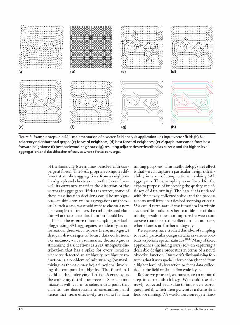
To illustrate SAL programming style, considerthe task of bundling vectors in a given vectorfield (for example, wind velocity or temperaturegradient) into a set of streamlines (paths throughthe field following the vector directions). Figure3 depicts this process; Figure 4 shows the corre-sponding SAL data mining program. This pro-gram has the following steps:

• (a) Establish a field that maps points (loca-tions) to points (vector directions, assumedhere to be normalized).

• (b) Localize computation with a neighborhoodgraph, so that only spatially proximate pointsare compared.

• (c-f) Use a series of local computations on thisrepresentation to find equivalence classes ofneighboring vectors with respect to vector di-rection.

• (g) Redescribe equivalence classes of vectorsinto more abstract streamline curves.

• (h) Aggregate and classify these curves intogroups with similar flow behavior, using theexact same operators but with different met-rics (code not shown).

As this example illustrates, SAL provides a vo-

cabulary for expressing the knowledge required(distance and similarity metrics) for uncoveringmultilevel structures in spatial data sets. Re-searchers have applied it to applications rangingfrom decentralized control design8 to analysis ofdiffusion-reaction morphogenesis.9

Data collection and samplingThe exploitation of physical properties is a

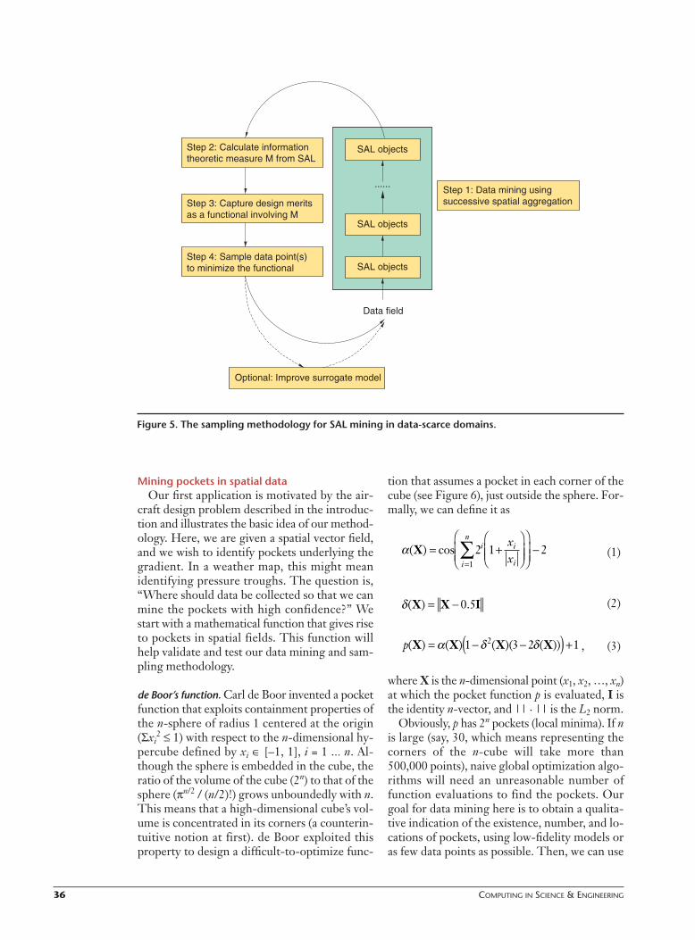
central tenet of SAL because it drives the com-putation of multilevel spatial aggregates. We canexpress many important physical properties asSAL computations by suitably defining adja-cency relations and aggregation metrics. To ex-tend SAL to data-scarce settings, we present thesampling methodology that Figure 5 outlines.

Once again, understanding the methodology inthe context of the vector field bundling applica-tion is easy (see Figure 3). Assume that we applyFigure 4’s SAL data mining program with a smalldata set and have navigated up to the highest level

Searchconsistent?

Disaggregate

Disaggregate

Lower-level objects

Classifygeometric opsMap, filter,

Higher-level objects

Input field

Aggregate

Structural description

Behavioral description

Abstract description

Redescribe

Redescribe

Updateobjects

N-graph

classesEquivalence

Spatial

Figure 2. The Spatial Aggregation Language’s multilayer spatial aggregates, uncovered by a uniform vocabulary of operators usingdomain knowledge. We can express several scientific data miningtasks—such as vector field bundling, contour aggregation,correspondence abstraction, clustering, and uncovering regions ofuniformity—as multilevel computations with SAL aggregates.

34 COMPUTING IN SCIENCE & ENGINEERING

of the hierarchy (streamlines bundled with con-vergent flows). The SAL program computes dif-ferent streamline aggregations from a neighbor-hood graph and chooses one on the basis of howwell its curvature matches the direction of thevectors it aggregates. If data is scarce, some ofthese classification decisions could be ambigu-ous—multiple streamline aggregations might ex-ist. In such a case, we would want to choose a newdata sample that reduces the ambiguity and clar-ifies what the correct classification should be.

This is the essence of our sampling method-ology: using SAL aggregates, we identify an in-formation-theoretic measure (here, ambiguity)that can drive stages of future data collection.For instance, we can summarize the ambiguousstreamline classifications as a 2D ambiguity dis-tribution that has a spike for every locationwhere we detected an ambiguity. Ambiguity re-duction is a problem of minimizing (or maxi-mizing, as the case may be) a functional involv-ing the computed ambiguity. The functionalcould be the underlying data field’s entropy, asthe ambiguity distribution reveals. Such a mini-mization will lead us to select a data point thatclarifies the distribution of streamlines, andhence that more effectively uses data for data

mining purposes. This methodology’s net effectis that we can capture a particular design’s desir-ability in terms of computations involving SALaggregates. Thus, sampling is conducted for theexpress purpose of improving the quality and ef-ficacy of data mining. The data set is updatedwith the newly collected value, and the processrepeats until it meets a desired stopping criteria.We could terminate if the functional is withinaccepted bounds or when confidence of datamining results does not improve between suc-cessive rounds of data collection—in our case,when there is no further ambiguity.

Researchers have studied this idea of samplingto satisfy particular design criteria in various con-texts, especially spatial statistics.10–12 Many of theseapproaches (including ours) rely on capturing adesirable design’s properties in terms of a novelobjective function. Our work’s distinguishing fea-ture is that it uses spatial information gleaned froma higher level of abstraction to focus data collec-tion at the field or simulation code layer.

Before we proceed, we must note an optionalstep in our methodology. We could use thenewly collected data value to improve a surro-gate model, which then generates a dense datafield for mining. We would use a surrogate func-

(e) (f) (g) (h)

(a) (b) (c) (d)

Figure 3. Example steps in a SAL implementation of a vector field analysis application. (a) Input vector field; (b) 8-adjacency neighborhood graph; (c) forward neighbors; (d) best forward neighbors; (e) N-graph transposed from bestforward neighbors; (f) best backward neighbors; (g) resulting adjacencies redescribed as curves; and (h) higher-level aggregation and classification of curves whose flows converge.

JULY/AUGUST 2002 35

tion in lieu of the real data source to generatesufficient data for mining purposes, which is of-ten more advantageous than working directlywith sparse data. Surrogate models are widelyused in engineering design, optimization, andresponse-surface approximations.13,14

Example applications

Together, SAL and our focused samplingmethodology address the main issues raised in the

beginning of this article: SAL’s uniform use of fieldsand abstraction operators lets us exploit priorknowledge in a bottom-up manner. The samplingmethodology uses discrepancies as suggested byour knowledge of physical properties in a top-down manner. Continuing these two stages alter-natively leads to a closed-loop data mining solu-tion for data-scarce domains (see Figure 5). Let’slook at two examples—mining pockets in spatialdata and qualitative determination of Jordan formsof matrices—that demonstrate this approach.

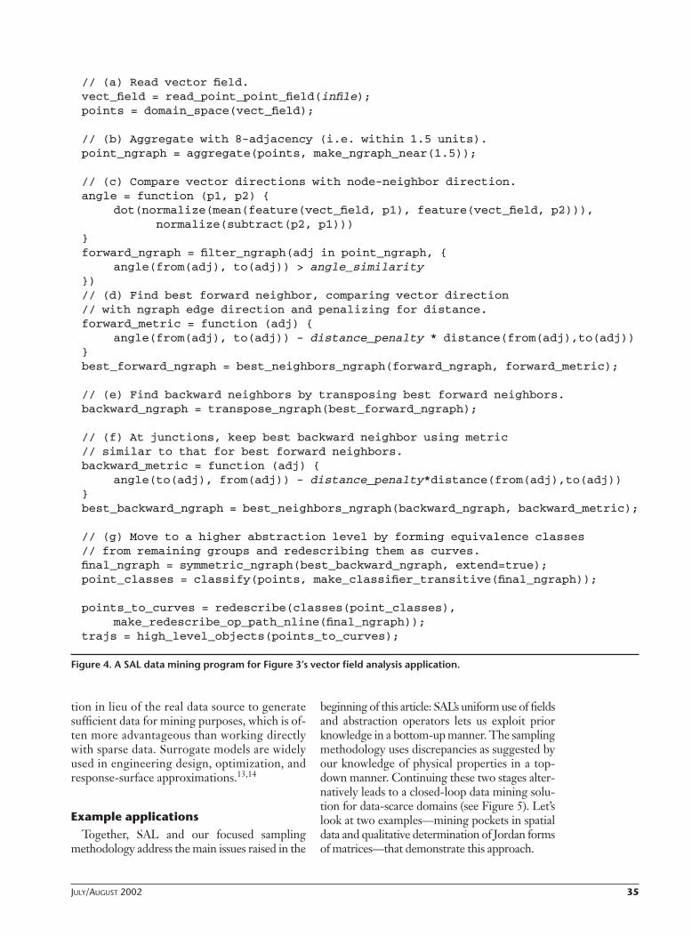
// (a) Read vector field.vect_field = read_point_point_field(infile);points = domain_space(vect_field);

// (b) Aggregate with 8-adjacency (i.e. within 1.5 units).point_ngraph = aggregate(points, make_ngraph_near(1.5));

// (c) Compare vector directions with node-neighbor direction.angle = function (p1, p2) {

dot(normalize(mean(feature(vect_field, p1), feature(vect_field, p2))),normalize(subtract(p2, p1)))

}forward_ngraph = filter_ngraph(adj in point_ngraph, {

angle(from(adj), to(adj)) > angle_similarity})// (d) Find best forward neighbor, comparing vector direction// with ngraph edge direction and penalizing for distance.forward_metric = function (adj) {

angle(from(adj), to(adj)) - distance_penalty * distance(from(adj),to(adj))}best_forward_ngraph = best_neighbors_ngraph(forward_ngraph, forward_metric);

// (e) Find backward neighbors by transposing best forward neighbors.backward_ngraph = transpose_ngraph(best_forward_ngraph);

// (f) At junctions, keep best backward neighbor using metric// similar to that for best forward neighbors.backward_metric = function (adj) {

angle(to(adj), from(adj)) - distance_penalty*distance(from(adj),to(adj))}best_backward_ngraph = best_neighbors_ngraph(backward_ngraph, backward_metric);

// (g) Move to a higher abstraction level by forming equivalence classes// from remaining groups and redescribing them as curves.final_ngraph = symmetric_ngraph(best_backward_ngraph, extend=true);point_classes = classify(points, make_classifier_transitive(final_ngraph));

points_to_curves = redescribe(classes(point_classes),make_redescribe_op_path_nline(final_ngraph));

trajs = high_level_objects(points_to_curves);

Figure 4. A SAL data mining program for Figure 3’s vector field analysis application.

36 COMPUTING IN SCIENCE & ENGINEERING

Mining pockets in spatial dataOur first application is motivated by the air-

craft design problem described in the introduc-tion and illustrates the basic idea of our method-ology. Here, we are given a spatial vector field,and we wish to identify pockets underlying thegradient. In a weather map, this might meanidentifying pressure troughs. The question is,“Where should data be collected so that we canmine the pockets with high confidence?” Westart with a mathematical function that gives riseto pockets in spatial fields. This function willhelp validate and test our data mining and sam-pling methodology.

de Boor’s function. Carl de Boor invented a pocketfunction that exploits containment properties ofthe n-sphere of radius 1 centered at the origin(Σxi

2 ≤ 1) with respect to the n-dimensional hy-percube defined by xi ∈ [–1, 1], i = 1 ... n. Al-though the sphere is embedded in the cube, theratio of the volume of the cube (2n) to that of thesphere (πn/2 / (n/2)!) grows unboundedly with n.This means that a high-dimensional cube’s vol-ume is concentrated in its corners (a counterin-tuitive notion at first). de Boor exploited thisproperty to design a difficult-to-optimize func-

tion that assumes a pocket in each corner of thecube (see Figure 6), just outside the sphere. For-mally, we can define it as

(1)

(2)

, (3)

where X is the n-dimensional point (x1, x2, …, xn)at which the pocket function p is evaluated, I isthe identity n-vector, and || · || is the L2 norm.

Obviously, p has 2n pockets (local minima). If nis large (say, 30, which means representing thecorners of the n-cube will take more than500,000 points), naive global optimization algo-rithms will need an unreasonable number offunction evaluations to find the pockets. Ourgoal for data mining here is to obtain a qualita-tive indication of the existence, number, and lo-cations of pockets, using low-fidelity models oras few data points as possible. Then, we can use

p( ) ( ) ( )( ( ))X X X X= − −( ) +α δ δ1 3 2 12

δ( ) .X X I= − 0 5

α( ) cosX = +

−

=∑2 1 2

1

i i

ii

n xx

Step 1: Data mining usingsuccessive spatial aggregationStep 3: Capture design merits

as a functional involving M

Optional: Improve surrogate model

......

SAL objects

SAL objects

SAL objects

Data field

to minimize the functional

Step 2: Calculate informationtheoretic measure M from SAL

Step 4: Sample data point(s)

Figure 5. The sampling methodology for SAL mining in data-scarce domains.

JULY/AUGUST 2002 37

the results to seed higher-fidelity calculations.This fundamentally differs from DACE (Designand Analysis of Computer Experiments),12 poly-nomial response surface approximations,13 andother approaches in geostatistics where the goalis accuracy of functional prediction at untesteddata points. Here, we trade accuracy of estima-tion for the ability to mine pockets.

Surrogate function. In this study, we use the SALvector field bundling code presented earlier alongwith a surrogate model as the basis for generatinga dense data field. Surrogate theory is an estab-lished area in engineering optimization, and wecan build a surrogate in several ways. However,the local nature of SAL computations means thatwe can be selective about our choice of surrogaterepresentation. For example, global, least-squarestype approximations are inappropriate becausemeasurements at all locations are equally consid-ered to uncover trends and patterns in a particu-lar region. We advocate the use of kriging-type in-terpolators,12 which are local modeling methodswith roots in Bayesian statistics. Kriging can han-dle situations with multiple local extrema and caneasily exploit anisotropies and trends. Given kobservations, the interpolated model gives exactresponses at these k sites and estimates values atother sites by minimizing the mean-squared er-ror (MSE), assuming a random data process withzero mean and a known covariance function.

Formally (for two dimensions), we assume thetrue function p to be the realization of a randomprocess such as

p(x, y) = β + Z(x, y), (4)

where β is typically a uniform random variate,estimated based on the known k values of p, andZ is a correlation function. Kriging then esti-mates a model p′ of the same form, on the basisof the k observations,

p′(xi, yi) = E( p(xi, yi) | p(x1, y1), ..., p(xk, yk)), (5)

and minimizing MSE between p′ and p,

MSE = E( p′(x, y) – p(x, y))2. (6)

A typical choice for Z in p′ is σ2 R, where scalarσ2 is the estimated variance, and correlation ma-trix R encodes domain-specific constraints andreflects the data’s current fidelity. We use an ex-ponential function for entries in R, with two pa-rameters C1 and C2:

. (7)

Intuitively, values at closer points should bemore highly correlated.

We get the MSE-minimizing estimator bymultidimensional optimization (the derivationfrom Equations 6 and 7 is beyond this article’sscope):

. (8)

This expression satisfies the conditions thatthere is no error between the model and the truevalues at the chosen k sites and that all variabilityin the model arises from the design of Z. Gradi-ent descent or pattern search methods often per-form the multidimensional optimization.12

Data mining and sampling methodology. The bot-tom-up computation of SAL aggregates fromthe surrogate model’s outputs will possibly leadto some ambiguous streamline classifications, aswe discussed earlier. Ambiguity can reflect thedesirability of acquiring data at or near a speci-fied point—to clarify the correct classificationand to serve as a mathematical criterion of in-formation content. We can use informationabout ambiguity to drive data collection in sev-eral ways. In this study, we express the ambigui-ties as a distribution describing the number ofpossible good neighbors. This ambiguity distri-

max ln ln

C

kR

−+( )2

2σ

R eijC x x C y yi j i j= − − − −1

22

2

–1–0.5

00.5

1

–1

–0.5

0

0.5

1–2

–1.5

–1

–0.5

0

0.5

1

Figure 6. A 2D pocket function.

38 COMPUTING IN SCIENCE & ENGINEERING

bution provides a novel mechanism to includequalitative information; streamlines that agreewill generally contribute less to data mining, forinformation purposes. We thus define the infor-mation-theoretic measure M (see Figure 5) to bethe ambiguity distribution ℘.

We define the functional as the posterior en-tropy E(–log d), where d is the conditional densityof ℘ over the design space not covered by thecurrent data values. By a reduction argument,minimizing this posterior entropy can be shownto maximize the prior entropy over the sampleddesign space.12 In turn, this maximizes theamount of information obtained from an experi-ment (additional data collection). Moreover, wealso incorporate ℘ as an indicator covarianceterm in our surrogate model, which is a conven-tional method for including qualitative informa-tion in an interpolatory model.11

Experimental results. Our initial experimentalconfiguration used a face-centered design (fourpoints, in the 2D case). A surrogate model bykriging interpolation then generated data on a41n-point grid. We used de Boor’s function asthe source for data values; we also employedpseudorandom perturbations of it that shift thepockets from the corners somewhat unpre-dictably.15 In total, we experimented with 200perturbed variations of the 2D and 3D pocketfunctions. For each of these cases, we organizeddata collection in rounds of one extra sampleeach (to minimize the functional). We recordedthe number of samples SAL needed to mine allthe pockets and compared our results with thoseobtained from a pure DACE–kriging approach.In other words, we used the DACE methodol-ogy to suggest new locations for data collectionand determined how those choices fared with re-spect to mining the pockets.

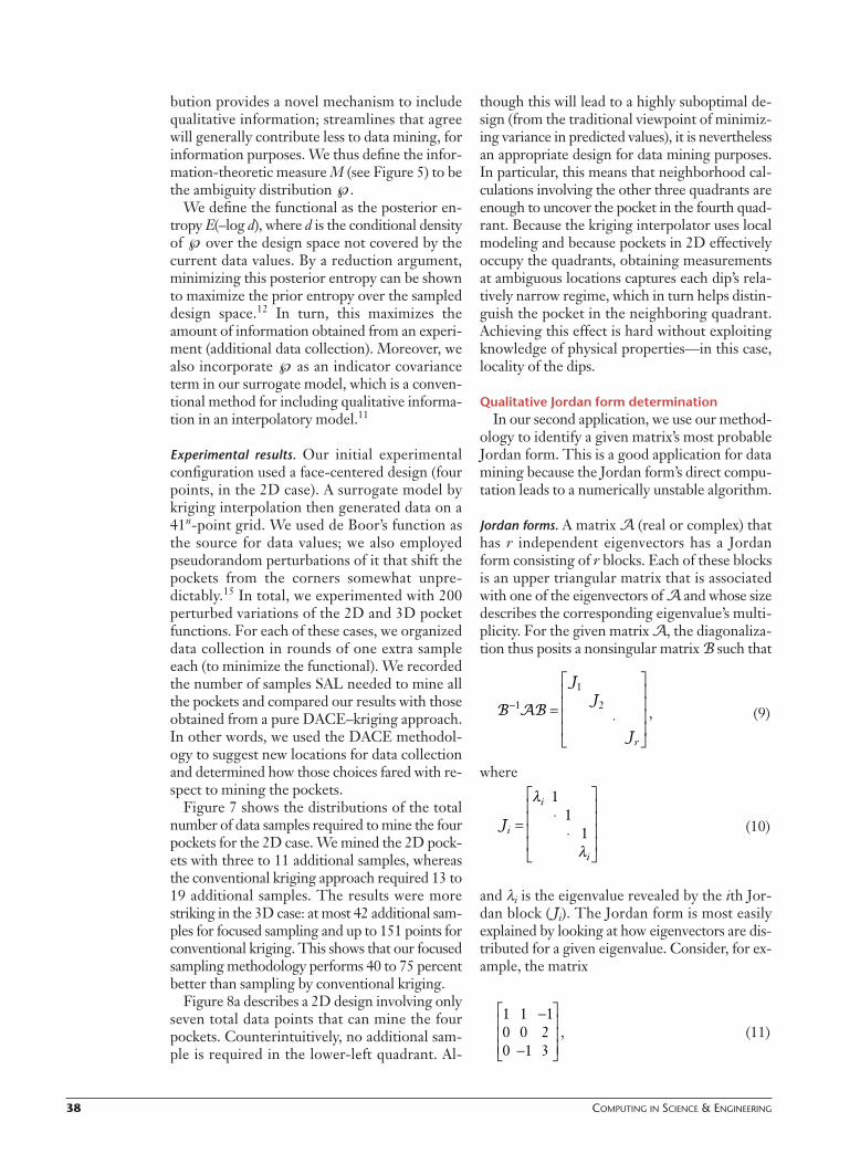
Figure 7 shows the distributions of the totalnumber of data samples required to mine the fourpockets for the 2D case. We mined the 2D pock-ets with three to 11 additional samples, whereasthe conventional kriging approach required 13 to19 additional samples. The results were morestriking in the 3D case: at most 42 additional sam-ples for focused sampling and up to 151 points forconventional kriging. This shows that our focusedsampling methodology performs 40 to 75 percentbetter than sampling by conventional kriging.

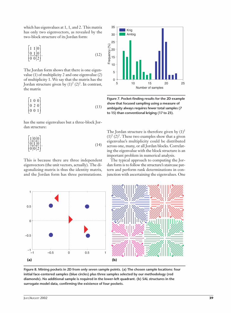
Figure 8a describes a 2D design involving onlyseven total data points that can mine the fourpockets. Counterintuitively, no additional sam-ple is required in the lower-left quadrant. Al-

though this will lead to a highly suboptimal de-sign (from the traditional viewpoint of minimiz-ing variance in predicted values), it is neverthelessan appropriate design for data mining purposes.In particular, this means that neighborhood cal-culations involving the other three quadrants areenough to uncover the pocket in the fourth quad-rant. Because the kriging interpolator uses localmodeling and because pockets in 2D effectivelyoccupy the quadrants, obtaining measurementsat ambiguous locations captures each dip’s rela-tively narrow regime, which in turn helps distin-guish the pocket in the neighboring quadrant.Achieving this effect is hard without exploitingknowledge of physical properties—in this case,locality of the dips.

Qualitative Jordan form determinationIn our second application, we use our method-

ology to identify a given matrix’s most probableJordan form. This is a good application for datamining because the Jordan form’s direct compu-tation leads to a numerically unstable algorithm.

Jordan forms. A matrix A (real or complex) thathas r independent eigenvectors has a Jordanform consisting of r blocks. Each of these blocksis an upper triangular matrix that is associatedwith one of the eigenvectors of A and whose sizedescribes the corresponding eigenvalue’s multi-plicity. For the given matrix A, the diagonaliza-tion thus posits a nonsingular matrix B such that

, (9)

where

(10)

and λi is the eigenvalue revealed by the ith Jor-dan block (Ji). The Jordan form is most easilyexplained by looking at how eigenvectors are dis-tributed for a given eigenvalue. Consider, for ex-ample, the matrix

, (11)

1 1 10 0 20 1 3

−

−

Ji

i

i

=⋅

⋅

λ

λ

11

1

B ABJ

J

J

− = ⋅

1

1

2

r

JULY/AUGUST 2002 39

which has eigenvalues at 1, 1, and 2. This matrixhas only two eigenvectors, as revealed by thetwo-block structure of its Jordan form:

. (12)

The Jordan form shows that there is one eigen-value (1) of multiplicity 2 and one eigenvalue (2)of multiplicity 1. We say that the matrix has theJordan structure given by (1)2 (2)1. In contrast,the matrix

(13)

has the same eigenvalues but a three-block Jor-dan structure:

. (14)

This is because there are three independenteigenvectors (the unit vectors, actually). The di-agonalizing matrix is thus the identity matrix,and the Jordan form has three permutations.

The Jordan structure is therefore given by (1)1

(1)1 (2)1. These two examples show that a giveneigenvalue’s multiplicity could be distributedacross one, many, or all Jordan blocks. Correlat-ing the eigenvalue with the block structure is animportant problem in numerical analysis.

The typical approach to computing the Jor-dan form is to follow the structure’s staircase pat-tern and perform rank determinations in con-junction with ascertaining the eigenvalues. One

1 0 00 1 00 0 2

1 0 00 2 00 0 1

1 1 00 1 00 0 2

10 15Number of samples

20 250

5

10

15

20

25

5

30

35

Fre

quen

cy (

%)

Krig Ambig

Figure 7. Pocket-finding results for the 2D exampleshow that focused sampling using a measure ofambiguity always requires fewer total samples (7to 15) than conventional kriging (17 to 23).

–1 –0.5 0 0.5 1–1

–0.5

0

0.5

1

(a) (b)

Figure 8. Mining pockets in 2D from only seven sample points. (a) The chosen sample locations: fourinitial face-centered samples (blue circles) plus three samples selected by our methodology (reddiamonds). No additional sample is required in the lower-left quadrant. (b) SAL structures in the surrogate model data, confirming the existence of four pockets.

40 COMPUTING IN SCIENCE & ENGINEERING

of the more serious caveats with such an ap-proach involves mistaking an eigenvalue of mul-tiplicity greater than 1 for multiple eigenval-ues.16 In Equation 11, this might lead toinferring that the Jordan form has three blocks.The extra care needed to safeguard staircase al-gorithms usually involves more complexity thanthe original computation to be performed. Theill-conditioned nature of this computation hasthus traditionally prompted numerical analyststo favor other, more stable, decompositions.

Qualitative assessment of Jordan forms. A recentdevelopment has been the acceptance of a quali-tative approach to Jordan structure determina-tion, proposed by Françoise Chaitin-Chatelinand Valerie Frayssé.17 This approach does not usethe staircase idea. Instead, it exploits a semanticsof eigenvalue perturbations to infer multiplicity,which leads to a geometrically intuitive algorithmthat we can implement using SAL.

Consider a matrix that has eigenvalues λ1, λ2,…, λn with multiplicities ρ1, ρ2, …, ρn. Any at-tempt at finding the eigenvalues (for example,determining the roots of the characteristic poly-nomial) is intrinsically subject to the numericalanalysis dogma: the problem being solved willactually be a perturbed version of the originalproblem. This allows the expression of the com-puted eigenvalues in terms of perturbations onthe actual eigenvalues. The computed eigen-value corresponding to any λk will be distributedon the complex plane as

, (15)

where the phase φ of the perturbation ∆ rangesover {2π, 4π, …, 2ρk π} if ∆ is positive and over{3π, 5π, …, 2(ρk + 1)π} if ∆ is negative. Chaitin-Chatelin and Frayssé superimposed numeroussuch perturbed calculations graphically so thatthe aggregate picture reveals the ρk of the eigen-value λk.17 The phase variations imply that thecomputed eigenvalues will lie on a regular poly-gon’s vertices—centered on the actual eigen-value—where the number of sides is two timesthe multiplicity of the considered eigenvalue.This takes into account both positive and nega-tive ∆. Because ∆ influences the polygon’s diam-eter, iterating this process over many ∆ will leadto a “sticks” depiction of the Jordan form.

To illustrate, we choose a matrix whose com-putations will be more prone to finite precision

errors. Perturbations on the 8 × 8 Brunet matrixwith Jordan structure (–1)1 (–2)1 (7)3 (7)3 inducethe superimposed structures in Figure 9.17 Fig-ure 9a depicts normwise relative perturbationsin the scale of [2–50, 2–40]. The six sticks aroundthe eigenvalue at 7 clearly reveal that its Jordanblock is of size 3. The other Jordan block, alsocentered at 7, is revealed if we conduct our ex-ploration at a finer perturbation level. Figure 9breveals the second Jordan block using perturba-tions in the range [2–53, 2–50]. The noise in bothpictures is a consequence of having two Jordanblocks with the same size and a “ring” phenom-enon studied elsewhere.18 We do not attempt tocapture these effects in this article.

Data mining and sampling methodology. For thisstudy, we collect data by random normwise per-turbations in a given region, and a SAL programdetermines multiplicity by detecting symmetrycorrespondence in the samples. The first aggre-gation level collects a given perturbation’s sam-ples into triangles. The second aggregation levelfinds congruent triangles via geometric hash-ing19 and uses congruence to establish a corre-spondence relation among triangle vertices. Thisrelation is then abstracted into a rotation about apoint (the eigenvalue) and evaluated for whethereach point rotates onto another and whethermatches define regular polygons. A third levelthen compares rotations across different pertur-bations, revisiting perturbations or choosing newones to disambiguate (see Figure 10).

The end result of this analysis is a confidencemeasure on models of possible Jordan forms.Each model is defined by its estimate of λ and ρ(we work in one region at a time). The measureM is the joint probability distribution over thespace of λ and ρ.

Experimental results. Because our Jordan formcomputation treats multiple perturbations irre-spective of level as independent estimates ofeigenstructure, the idea of sampling here is notwhere to collect, but how much to collect. Thegoal of data mining is hence to improve our con-fidence in model evaluation.

We organized data collection into rounds ofsix to eight samples each, varied a tolerance pa-rameter for triangle congruence from 0.1 to 0.5(effectively increasing the number of modelsposited), and determined the number of roundsneeded to determine the Jordan form. As testcases, we used the set of matrices Chaitin-Chatelin and Frayssé studied.17 On average, our

λ ρ

φρ

k

i

k ke+ ∆1

JULY/AUGUST 2002 41

focused sampling approach required one roundof data collection at a tolerance of 0.1 and up to2.7 rounds at 0.5. Even with a large number ofmodels posited, additional data quickly weededout bad models. Figure 10 demonstrates thismechanism on the Brunet matrix discussed ear-lier for two sets of sample points. To the best ofour knowledge, this is the only known focusedsampling methodology for this domain; we areunable to present any comparisons. However, byharnessing domain knowledge about correspon-dences, we have arrived at an intelligent sam-pling methodology that resembles what a humanwould get from visual inspection.

Our methodology for mining in data-scarce domains has several intrinsicbenefits. First, it is based on a uni-form vocabulary of operators that a

rich diversity of applications can exploit. Second,it demonstrates a novel factorization to the prob-lem of mining when data is scarce—namely, for-mulating an experiment design methodology toclarify, disambiguate, and improve confidencesin higher-level aggregates of data. This lets usbridge qualitative and quantitative information

in a unified framework. Third, our methodologycan coexist with more traditional approaches toproblem solving (numerical analysis and opti-mization); it is not meant to be a replacement ora contrasting approach.

The methodology makes several intrinsic as-sumptions that we only briefly mention here.Both our applications have been such that thecause, formation, and effect of the relevant phys-ical properties are well understood. This is pre-cisely what lets us act decisively on the basis ofhigher-level information from SAL aggregates,through the measure M. It also assumes that theproblems the mining algorithm will encounterare the same as the problems for which it was de-signed. This is an inheritance from Bayesian in-ductive inference and leads to fundamental lim-itations on what we can do in such a setting. Forinstance, if new data does not help clarify an am-biguity, does the fault lie with the model or thedata? We can summarize this problem by sayingthat the approach requires strong a priori infor-mation about what is possible and what is not.

Nevertheless, by advocating targeted use ofdomain-specific knowledge and aiding qualita-tive model selection, our methodology is moreefficient at determining high-level models fromempirical data. Together, SAL and our informa-

6.998 6.9985 6.999 6.9995 7 7.0005 7.001 7.0015 7.002-1.5

-1

-0.5

0

0.5

1

1.5x 10

–3

6.9998 6.9999 6.9999 7 7 7.0001 7.0001 7.0002 7.0002

-1

-0.5

0

0.5

1

1.5x 10

–4

(a) (b)

Figure 9. Superimposed spectra for assessing the Jordan form of the Brunet matrix. We see two Jordan blocks ofmultiplicity 3 for eigenvalue 7, at (a) coarse and (b) fine perturbation levels.

42 COMPUTING IN SCIENCE & ENGINEERING

tion-theoretic measure M encapsulate knowl-edge about physical properties, which is whatmakes our methodology viable for data mining.In the future, we aim to characterize more for-mally the particular forms of domain knowledgethat help overcome sparsity and noise in scien-tific data sets.

We could also extend our framework to takeinto account the expense of data samples. If thecost of data collection is nonuniform across thedomain, then including this in the design of ourfunctional will let us trade the cost of gatheringinformation with the expected improvement inproblem-solving performance. This area of datamining is called active learning.

Data mining can sometimes be a controversialterm in a discipline that is used to mathematicalrigor; this is because it is often used synony-mously with “lack of a hypothesis or theory.”This need not be the case. Data mining can in-deed be sensitive to knowledge about the do-main, especially physical properties of the kindwe have harnessed here. As data mining applica-tions become more prevalent in science, theneed to incorporate a priori domain knowledgewill become even more important.

AcknowledgmentsThis work is supported in part by US National ScienceFoundation grants EIA-9984317 and EIA-0103660. Wethank John R. Rice, Feng Zhao, and Layne T. Watson fortheir helpful comments.

References1. A. Goel et al., “VizCraft: A Problem-Solving Environment for Air-

craft Configuration Design,” Computing in Science & Eng., vol. 3,no. 1, Jan./Feb. 2001, pp. 56–66.

2. N. Ramakrishnan and A.Y. Grama, “Mining Scientific Data,” Ad-vances in Computers, vol. 55, Sept. 2001, pp. 119–169.

3. C. Bailey-Kellogg, F. Zhao, and K. Yip, “Spatial Aggregation: Lan-guage and Applications,” Proc. 13th Nat’l Conf. Artificial Intelli-gence (AAAI 96), AAAI Press, Menlo Park, Calif., 1996, pp.517–522.

4. V. Ganti, J. Gehrke, and R. Ramakrishnan, “Mining Very LargeDatabases,” Computer, vol. 32, no. 8, Aug. 1999, pp. 38–45.

5. J. Kivinen and H. Mannila, “The Use of Sampling in KnowledgeDiscovery,” Proc. 13th ACM Symp. Principles of Database Systems,ACM Press, New York, 1994, pp. 77–85.

6. K.M. Yip and F. Zhao, “Spatial Aggregation: Theory and Appli-cations,” J. Artificial Intelligence Research, vol. 5, 1996, pp. 1–26.

7. K.M. Yip, F. Zhao, and E. Sacks, “Imagistic Reasoning,” ACMComputing Surveys, vol. 27, no. 3, Sept. 1995, pp. 363–365.

8. C. Bailey-Kellogg and F. Zhao, “Influence-Based Model Decom-position for Reasoning about Spatially Distributed Physical Sys-tems,” Artificial Intelligence, vol. 130, no. 2, Aug. 2001, pp.125–166.

0.1

6.9 7.0 7.1–0.1

0

–0.1

0

0.1

6.9 7.0 7.1(a) (b)

(c)

0.1

6.9 7.0 7.1–0.1 –0.1

0.1

6.9 7.0 7.1(d)

00

Figure 10. Mining Jordan forms from a small ((a) and (c)) sample set and a larger ((b) and (d)) sampleset. Sections (a) and (b) depict selected approximately congruent triangles; (c) and (d) evaluate thecorrespondence of the original sample points with their images under a rotation aligning the triangles.

9. I. Ordóñez and F. Zhao, “Spatio-Temporal Aggregation with Ap-plications to Analysis of Diffusion-Reaction Phenomena,” Proc.17th Nat’l Conf. Artificial Intelligence (AAAI 00), AAAI Press, MenloPark, Calif., 2000, pp. 517–523.

10. R.G. Easterling, “Comment on ‘Design and Analysis of ComputerExperiments,’” Statistical Science, vol. 4, no. 4, Nov. 1989, pp.425–427.

11. A. Journel, “Constrainted Interpolation and Qualitative Informa-tion: The Soft Kriging Approach,” Mathematical Geology, vol. 18,no. 2, Nov. 1986, pp. 269–286.

12. J. Sacks et al., “Design and Analysis of Computer Experiments,”Statistical Science, vol. 4, no. 4, Nov. 1989, pp. 409–423.

13. D.L. Knill et al., “Response Surface Models Combining Linear andEuler Aerodynamics for Supersonic Transport Design,” J. Aircraft,vol. 36, no. 1, Jan. 1999, pp. 75–86.

14. R.H. Myers and D.C. Montgomery, Response Surface Methodol-ogy: Process and Product Optimization Using Designed Experiments,John Wiley & Sons, New York, 2002.

15. C. Bailey-Kellogg and N. Ramakrishnan, “Ambiguity-DirectedSampling for Qualitative Analysis of Sparse Data from SpatiallyDistributed Physical Systems,” Proc. 17th Int’l Joint Conf. ArtificialIntelligence (IJCAI 01), Morgan Kaufmann, San Francisco, 2001,pp. 43–50.

16. A. Edelman and Y. Ma, “Staircase Failures Explained by Orthog-onal Versal Forms,” SIAM J. Matrix Analysis and Applications, vol.21, no. 3, 2000, pp. 1004–1025.

17. F. Chaitin-Chatelin and V. Frayssé, Lectures on Finite PrecisionComputations, Soc. For Industrial and Applied Mathematics,Monographs, Philadelphia, 1996.

18. A. Edelman and Y. Ma, “Non-Generic Eigenvalue Perturbations ofJordan Blocks,” Linear Algebra & Applications, vol. 273, nos. 1–3,Apr. 1998, pp. 45–63.

19. Y. Lamdan and H. Wolfson, “Geometric Hashing: A General andEfficient Model-Based Recognition Scheme,” Proc. 2nd Int’l Conf.Computer Vision (ICCV), IEEE CS Press, Los Alamitos, Calif., 1988,pp. 238–249.

Naren Ramakrishnan is an assistant professor of com-puter science at Virginia Tech. His research interests in-clude problem-solving environments, mining scientificdata, and personalization. He received his PhD in com-puter sciences from Purdue University. Contact him atthe Dept. of Computer Science, 660 McBryde Hall, Vir-ginia Tech, Blacksburg, VA 24061; naren@cs.vt.edu.

Chris Bailey-Kellogg is an assistant professor of com-puter sciences at Purdue. His research combines geo-metric, symbolic, and numeric approaches for dataanalysis and experiment planning in scientific and en-gineering domains. He received his BS and MS in elec-trical engineering and computer science from MIT andhis PhD in computer and information science fromOhio State University. Contact him at the Dept. ofComputer Sciences, 1398 Computer Science Bldg.,Purdue Univ., West Lafayette, IN 47907; cbk@cs.purdue.edu.

For more information on this or any other computingtopic, please visit our Digital Library at http://computer.org/publications/dlib.

JULY/AUGUST 2002

Member SocietiesAmerican Physical SocietyOptical Society of AmericaAcoustical Society of AmericaThe Society of RheologyAmerican Association of Physics TeachersAmerican Crystallographic AssociationAmerican Astronomical SocietyAmerican Association of Physicists in MedicineAVSAmerican Geophysical UnionOther Member OrganizationsSigma Pi Sigma, Physics Honor SocietySociety of Physics StudentsCorporate Associates

The American Institute of Physics is a not-for-profit mem-bership corporation chartered in New York State in 1931for the purpose of promoting the advancement and diffusionof the knowledge of physics and its application to humanwelfare. Leading societies in the fields of physics,astronomy, and related sciences are its members.

The Institute publishes its own scientific journals as well asthose of its Member Societies; provides abstracting and in-dexing services; provides online database services; dissem-inates reliable information on physics to the public; collectsand analyzes statistics on the profession and on physics edu-cation; encourages and assists in the documentation andstudy of the history and philosophy of physics; cooperateswith other organizations on educational projects at all levels;and collects and analyzes information on Federal programsand budgets.

The scientists represented by the Institute through itsMember Societies number approximately 120,000. In ad-dition, approximately 5,400 students in over 600 collegesand universities are members of the Institute’s Society ofPhysics Students, which includes the honor society SigmaPi Sigma. Industry is represented through 47 CorporateAssociates members.

Governing Board*John A. Armstrong, (Chair), Marc H. Brodsky (Executive Di-rector), Benjamin B. Snavely (Secretary), Martin Blume (APS),William F. I. Brinkman (APS), Judy R. Franz (APS),DonaldR. Hamann (APS), Myriam P. Sarachik (APS), Thomas J.McIlrath (APS), George H. Trilling (APS), Michael D. Duncan(OSA), Ivan P. Kaminow (OSA), Anthony M. Johnson (OSA),Elizabeth A. Rogan (OSA), Anthony A. Atchley (ASA),Lawrence A. Crum (ASA), Charles E. Schmid (ASA), ArthurB. Metzner (SOR), Christopher J. Chiaverina (AAPT),Charles H. Holbrow (AAPT), John Hubisz (AAPT), BernardV. Khoury (AAPT), Charlotte Lowe-Ma (ACA), S. NarasingaRao (ACA), Leonard V. Kuhi (AAS), Arlo U. Landolt (AAS),Robert W. Milkey (AAS), James B. Smathers (AAPM),Christopher H. Marshall (AAPM), Rudolf Ludeke (AVS), N.Rey Whetten (AVS), Dawn A. Bonnell (AVS), James L. Burch(AGU), Robert E. Dickinson (AGU), Jeffrey J. Park (AGU),Judy C. Holoviak (AGU), Louis J. Lanzerotti (AGU), FredSpilhaus (AGU), Brian Clark (2002) MAL, Frank L. Huband(MAL)*Executive Committee members are printed in italics.

Management CommitteeMarc H. Brodsky, Executive Director and CEO; RichardBaccante, Treasurer and CFO; Theresa C. Braun, VicePresident, Human Resources; James H. Stith, VicePresident, Physics Resources; Darlene A. Walters, SeniorVice President, Publishing; Benjamin B. Snavely, Secretary

Subscriber ServicesAIP subscriptions, renewals, address changes, andsingle-copy orders should be addressed to Circulation andFulfillment Division, American Institute of Physics, 1NO1,2 Huntington Quadrangle, Melville, NY 11747-4502. Tel.(800) 344-6902; e-mail subs@aip.org. Allow at least sixweeks’ advance notice. For address changes please send bothold and new addresses, and, if possible, include an addresslabel from the mailing wrapper of a recent issue.