1

Sampling in 2D

2

Sampling in 1D

t

f(t)

( )[ ] ( ) ( )s sk

f k f kT f t t kTδ= = −∑

k

f(t)

Continuous time signal

Discrete time signal

comb

3

Nyquist theorem (1D)

At least 2 sample/period are needed to represent a periodic signal

max

max

1 222 2

s

ss

T

T

πωπω ω

≤

= ≥

4

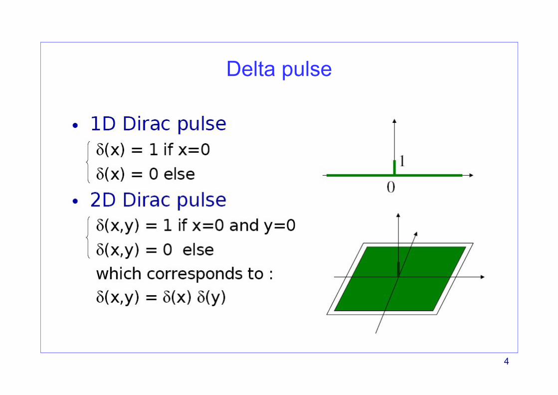
Delta pulse

5

Dirac brush

6

Comb

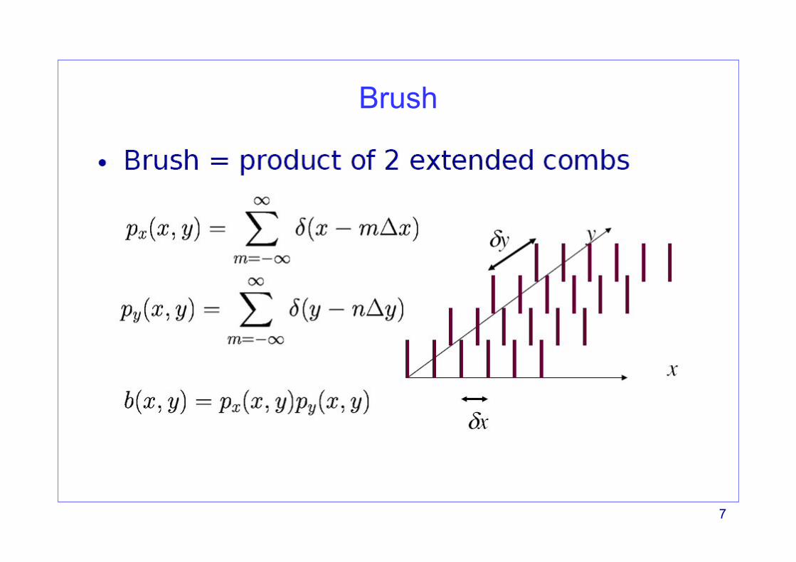
7

Brush

8

Nyquist theorem

• Sampling in p-dimensions

• Nyquist theorem

)()()(

)()(

xsxfxf

kTxxs

TT

ZkT

p

=

−= ∑∈

δTs

y

2D spatial domain

2D Fourier domain

ω x

ωy

ωxmax

ωymax

max max

max

max

122 2

12 22

sxs

x x xs

sy yy

y

T

T

πω ω ωω ω π

ω

⎧ ≤⎪⎧ ≥⎪ ⎪⇒⎨ ⎨≥⎪⎩ ⎪ ≤⎪⎩

Tsx

9

Spatial aliasing

10

Resampling

• Change of the sampling rate– Increase of sampling rate: Interpolation or upsampling

• Blurring, low visual resolution– Decrease of sampling rate: Rate reduction or downsampling

• Aliasing and/or loss of spatial details

11

Downsampling

12

Upsampling

nearest neighbor (NN)

13

Upsampling

bilinear

14

Upsampling

bicubic

15

Quantization

16

Scalar quantization

• A scalar quantizer Q approximates X by X˜=Q(X), which takes its values over a finite set.

• The quantization operation can be characterized by the MSE between theoriginal and the quantized signals

• Suppose that X takes its values in [a, b], which may correspond to thewhole real axis. We decompose [a, b] in K intervals {( yk-1, yk]}1≤k ≤ K ofvariable length, with y0=a and yK=b.

• A scalar quantizer approximates all x ∈( yk-1, yk] by xk:

( ] ( )1, ,k k kx y y Q x x−∀ ∈ =

17

Scalar quantization

• The intervals (yk-1, yk] are called quantization bins.

• Rounding off integers is an example where the quantization bins

(yk-1, yk]=(k-1/2, k+1/2]

have size 1and xk=k for any k∈Z.

• qui

• High resolution quantization– Let p(x) be the probability density of the random source X. The mean-square

quantization error is

18

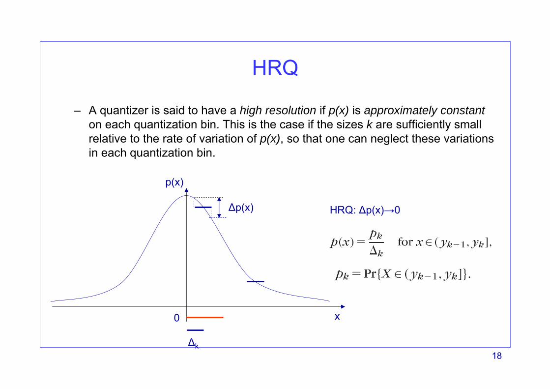
HRQ

– A quantizer is said to have a high resolution if p(x) is approximately constanton each quantization bin. This is the case if the sizes k are sufficiently small relative to the rate of variation of p(x), so that one can neglect these variations in each quantization bin.

x

p(x)

0

Δp(x)

Δk

HRQ: Δp(x)→0

19

Scalar quantization

• Teorem 10.4 (Mallat): For a high-resolution quantizer, the mean-square error d is minimized when xk=(yk+yk+1)/2, which yields

2

1

112

K

k kk

d p=

= Δ∑

20

Uniform quantizer

21

Quantization

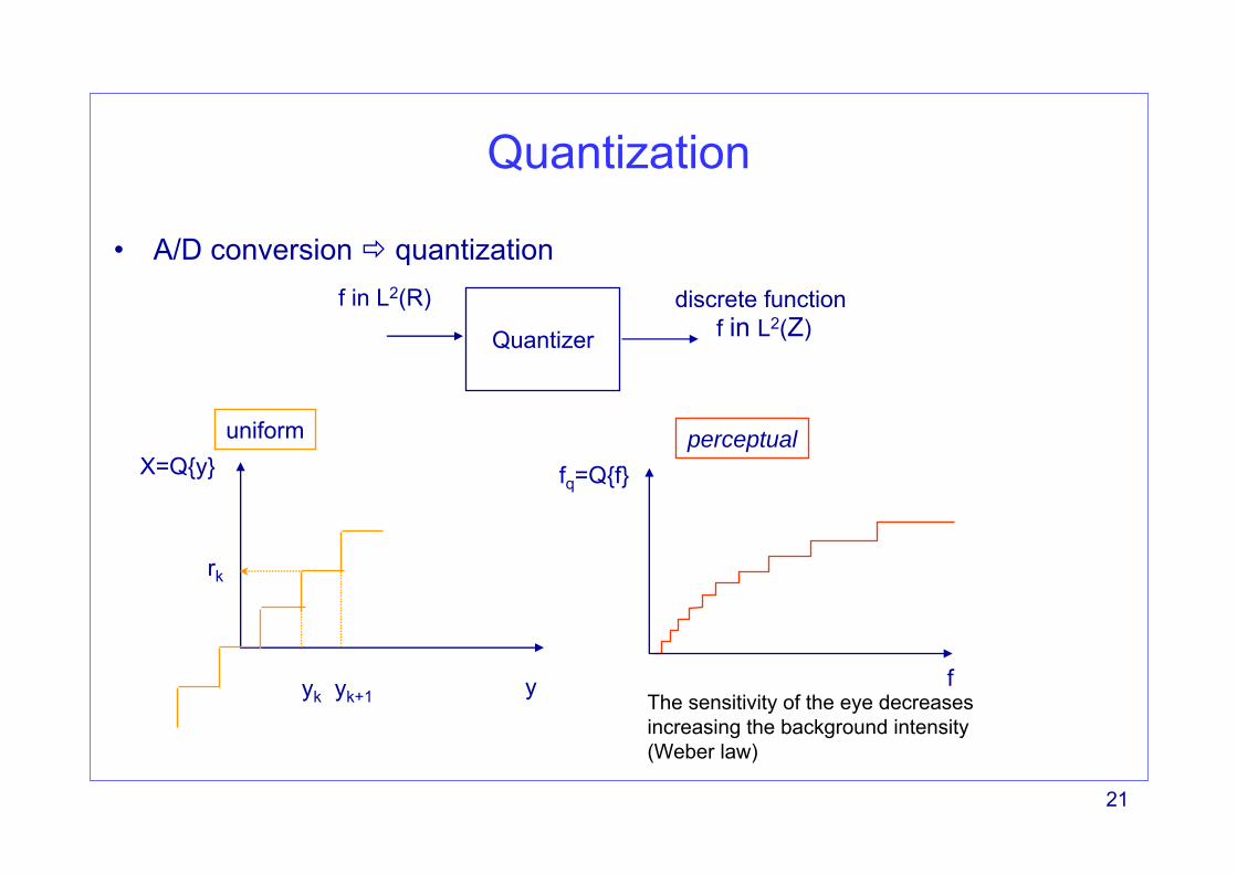
• A/D conversion quantization

Quantizer

f in L2(R) discrete functionf in L2(Z)

X=Q{y}

yyk yk+1

uniform perceptual

rk

fq=Q{f}

fThe sensitivity of the eye decreases increasing the background intensity (Weber law)

22

Quantization

Signal before (blue) and after quantization (red) Q

Equivalent noise: n=fq- f

additive noise model: fq=f+n

23

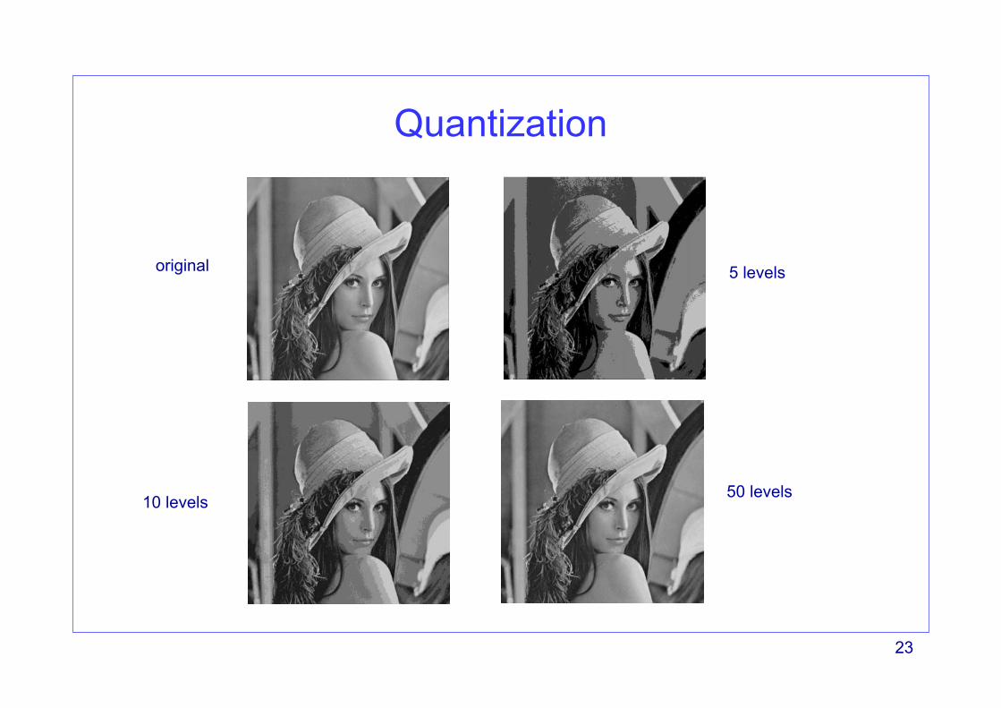
Quantization

original 5 levels

10 levels 50 levels

24

Distortion measure• Distortion measure

– The distortion is measured as the expectation of the mean square error (MSE) difference between the original and quantized signals.

• Lack of correlation with perceived image quality– Even though this is a very natural way for the quantification of the quantization artifacts,

it is not representative of the visual annoyance due to the majority of common artifacts.

• Visual models are used to define perception-based image quality assessment metrics

( )[ ] ( )∑ ∫=

+

−=−Ε=K

k

t

tQQ

k

k

dffpffffD0

221

)(

[ ] [ ]( )10 10

21 2

1 1

255 25520log 20log1 , ,

N M

i j

PSNRMSE

I i j I i jN M = =

= =

−× ∑∑

25

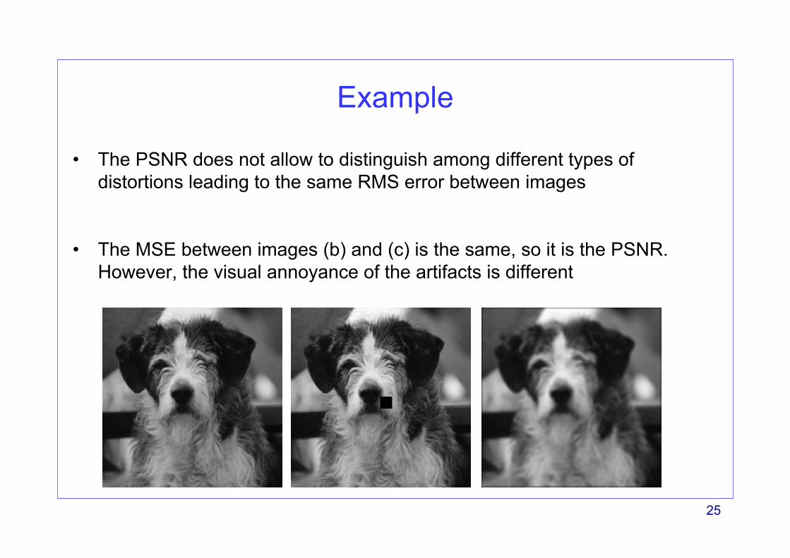
Example

• The PSNR does not allow to distinguish among different types of distortions leading to the same RMS error between images

• The MSE between images (b) and (c) is the same, so it is the PSNR. However, the visual annoyance of the artifacts is different

26

Convolution

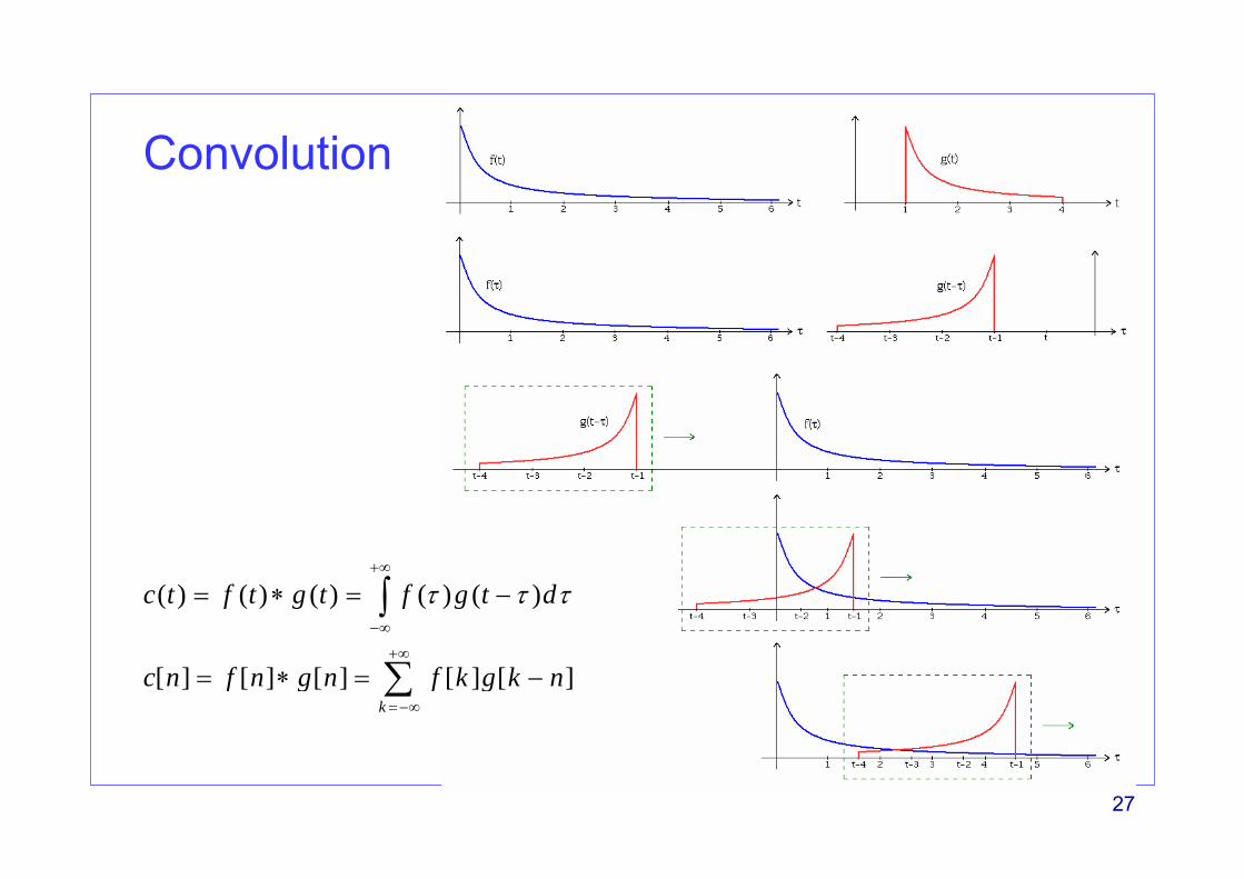
27

Convolution

( ) ( ) ( ) ( ) ( )

[ ] [ ] [ ] [ ] [ ]k

c t f t g t f g t d

c n f n g n f k g k n

τ τ τ+∞

−∞

+∞

=−∞

= ∗ = −

= ∗ = −

∫

∑

28

( , ) ( , ) ( , ) ( , ) ( , )

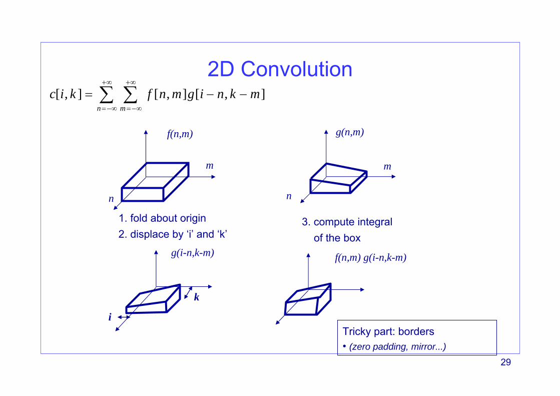
[ , ] [ , ] [ , ]n m

c x y f x y g x y f g x y d d

c i k f n m g i n k m

τ ν τ ν τ ν+∞ +∞

−∞ −∞

+∞ +∞

=−∞ =−∞

= ⊗ = − −

= − −

∫ ∫

∑ ∑

[n,m]

filter impulse response rotated by 180 deg

2D Convolution

• Associativity

• Commutativity

• Distributivity

29

g(n,m)

f(n,m) g(i-n,k-m)

1. fold about origin2. displace by ‘i’ and ‘k’

f(n,m)

m

n

g(i-n,k-m)

i

k

Tricky part: borders• (zero padding, mirror...)

3. compute integralof the box

2D Convolution[ , ] [ , ] [ , ]

n m

c i k f n m g i n k m+∞ +∞

=−∞ =−∞

= − −∑ ∑

m

n

30

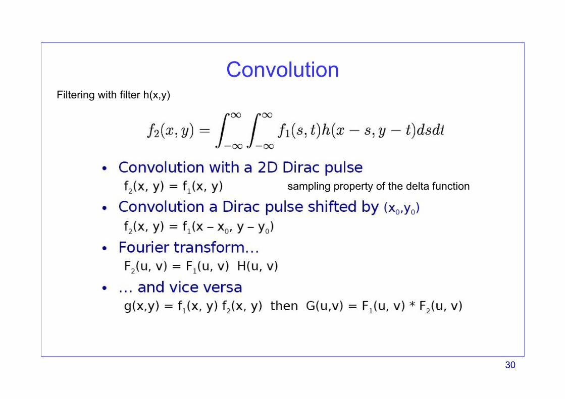
ConvolutionFiltering with filter h(x,y)

sampling property of the delta function

31

Convolution

• Convolution is a neighborhood operation in which each output pixel is the weighted sum of neighboring input pixels. The matrix of weights is called the convolution kernel, also known as the filter. – A convolution kernel is a correlation kernel that has been rotated 180 degrees.

• Recipe1. Rotate the convolution kernel 180 degrees about its center element. 2. Slide the center element of the convolution kernel so that it lies on top of the

(I,k) element of f. 3. Multiply each weight in the rotated convolution kernel by the pixel of f

underneath. Sum the individual products from step 3

– zero-padding is generally used at borders but other border conditions are possible

32

Examplef = [17 24 1 8 15

23 5 7 14 164 6 13 20 22

10 12 19 21 311 18 25 2 9]

h = [8 1 63 5 74 9 2]

h’= [2 9 47 5 36 1 8]

kernel

33

Correlation

• The operation called correlation is closely related to convolution. In correlation, the value of an output pixel is also computed as a weighted sum of neighboring pixels.

• The difference is that the matrix of weights, in this case called the correlation kernel, is not rotated during the computation.

• Recipe 1. Slide the center element of the correlation kernel so that lies on top of the

(2,4) element of f. 2. Multiply each weight in the correlation kernel by the pixel of A underneath. 3. Sum the individual products from step 2.

34

Examplef = [17 24 1 8 15

23 5 7 14 164 6 13 20 22

10 12 19 21 311 18 25 2 9]

h = [8 1 63 5 74 9 2]

kernel