Sampling, Beats, and the Software Oscilloscope∗

J. S. Freudenberg

EECS 461Embedded Control Systems

1 Introduction

As part of Lab 3, students use the ADC on the NXP S32K to periodically sample sine waves of variousfrequencies that are produced by a signal generator. The results are then displayed on a software oscilloscope.Depending on the frequency of the sine wave relative to the sampling frequency, the sampled signal can be avery good representation of the analog signal, or a very poor one. Even when the frequency of the sampledsignal lies below the Nyquist frequency, it may happen that the signal displayed on the oscilloscope appearsto be considerably distorted compared to the original analog signal. In particular, the sampled signal mayexhibit a phenomenon termed beats, a type of low frequency behavior that may appear to be present in asignal even though the signal does not, in fact, contain this frequency.

In this set of notes we use MATLAB to simulate the plots will see on the software oscilloscope, andexplain why they have the appearance that they do. It is important that students examine the plots, sothat they will know what to expect in the lab. Those so interested are encouraged to study the mathematicsbehind the phenomena.

Suppose we sample a sine of frequency f0 Hz,

f(t) = sin(2πf0t), (1)

with a sample period T seconds:f(kT ) = sin(2πf0kT ). (2)

Define the sampling frequency fs = 1/T Hz, the Nyquist frequency fN = 1/2T Hz, and the baseband orNyquist range ΩN = (−fN , fN ). It follows from the Shannon sampling theorem that if f0 ∈ ΩN , then inprinciple it is possible to perfectly reconstruct the signal (1) from its samples. Otherwise, the sine wave willappear, after sampling, to have a lower frequency than did the original analog signal. This is the phenomenonknown as aliasing.

Perfect reconstruction is not feasible in practice because it replaces requires all past and future valuesof the sampled signal. Instead, an approximate reconstruction scheme must be implemented. The softwareoscilloscope used in Lab 3 simply interpolates straight lines between successive sample points. Intuitionsuggests that if the sampling frequency is sufficiently larger than that of the sampled signal, then thereconstructed signal should closely resemble the original sine wave. If sampling is not sufficiently fast,then the reconstructed signal may be considerably distorted with respect to the original signal, even if theconditions of the Shannon sampling theorem are satisfied. As we shall see, the reason for the distortion lieswith the reconstruction scheme used.

The remainder of these notes are outlined as follows. In Section 2, we shall see several examples illustratingwhat you will see in Lab 3, including the beating phenomenon alluded to above. In Section 3, we shall reviewthe concept of continuous-time beats familiar from acoustics. We will then examine the frequency spectrumof the sampled signal to see how beats arise when imperfect reconstruction is applied to a signal that satisfiesthe Shannon sampling theorem.

∗Revised August 28, 2019.

1

2 Examples

The phenomena we study will depend on the relative values of the signal frequency and the samplingfrequency, and the examples in this section will be stated that way. The samples collected in Lab 3 will usea 50kHz sampling frequency.

2.1 Signal Frequency Much Less Than the Nyquist Frequency

If the Nyquist frequency is large, say 10 times the signal frequency, then the samples displayed on theoscilloscope should look much like the original signal. If the Nyquist frequency is closer, say 5 times thesignal frequency, some distortion will occur but the signal will have the same basic shape.

Example 1 Let the signal (1) have frequency f0 = 0.2fs Hz (period 5T seconds). The original signal,together with the samples, is displayed in the top plot of Figure 1, and the middle plot of Figure 1 containsthe samples interpolated with straight lines1. These plots show that the samples represent the signal withsome distortion; for example, the samples miss the peaks in the signal. However, even with the distortion, thesignal clearly has period 5T seconds and frequency 0.2fs Hz. The discrete time Fourier transform (DTFT)of the sampled signal, displayed in the bottom plot of Figure 1, shows peaks at ±0.2fs Hz, as expected.

0 5 10 15 20 25 30 35 40 45 50−1

0

1

normalized time, t/T

f0 = 0.2 f

s

0 5 10 15 20 25 30 35 40 45 50−1

0

1

normalized time, t/T

−0.5 −0.4 −0.3 −0.2 −0.1 0 0.1 0.2 0.3 0.4 0.50

200

400

600

normalized frequency, f/fs

DT

FT

Figure 1: (Top) Plots of sin(2πf0t) and sin(2πf0kT ) for f0 = 0.2fs Hz; (Middle) Plots of sin(2πf0kT ) withstraight lines interpolated between samples; (Bottom) Discrete time Fourier transform of sin(2πf0kT ).

1Figures 1-5 are generated with Matlab file plots Lab3 notes.m.

2

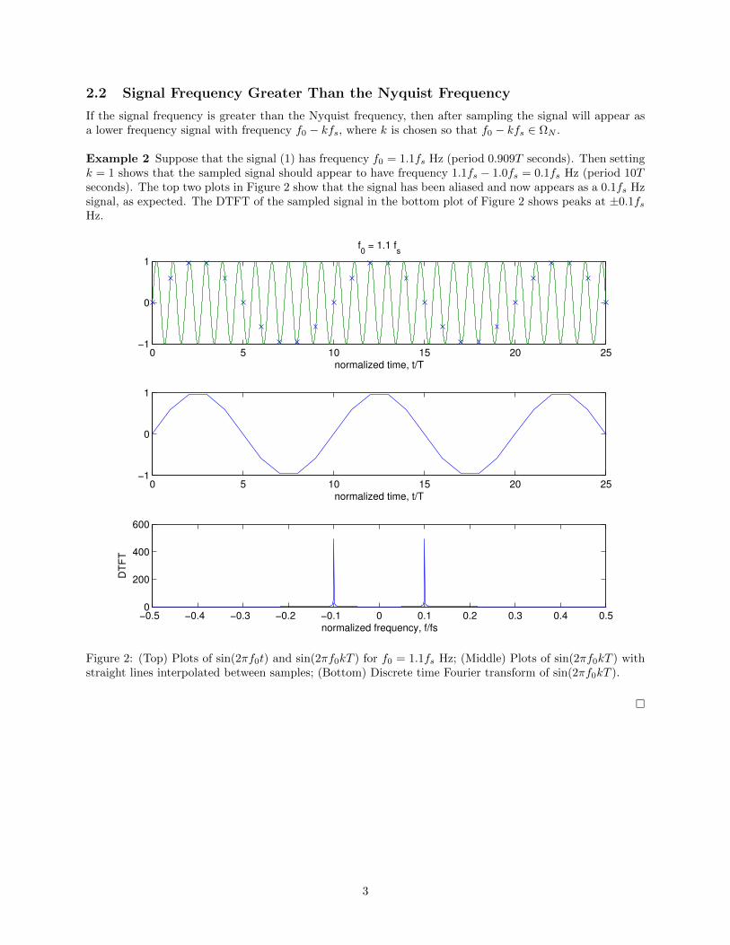
2.2 Signal Frequency Greater Than the Nyquist Frequency

If the signal frequency is greater than the Nyquist frequency, then after sampling the signal will appear asa lower frequency signal with frequency f0 − kfs, where k is chosen so that f0 − kfs ∈ ΩN .

Example 2 Suppose that the signal (1) has frequency f0 = 1.1fs Hz (period 0.909T seconds). Then settingk = 1 shows that the sampled signal should appear to have frequency 1.1fs − 1.0fs = 0.1fs Hz (period 10Tseconds). The top two plots in Figure 2 show that the signal has been aliased and now appears as a 0.1fs Hzsignal, as expected. The DTFT of the sampled signal in the bottom plot of Figure 2 shows peaks at ±0.1fsHz.

0 5 10 15 20 25−1

0

1

normalized time, t/T

f0 = 1.1 f

s

0 5 10 15 20 25−1

0

1

normalized time, t/T

−0.5 −0.4 −0.3 −0.2 −0.1 0 0.1 0.2 0.3 0.4 0.50

200

400

600

normalized frequency, f/fs

DT

FT

Figure 2: (Top) Plots of sin(2πf0t) and sin(2πf0kT ) for f0 = 1.1fs Hz; (Middle) Plots of sin(2πf0kT ) withstraight lines interpolated between samples; (Bottom) Discrete time Fourier transform of sin(2πf0kT ).

3

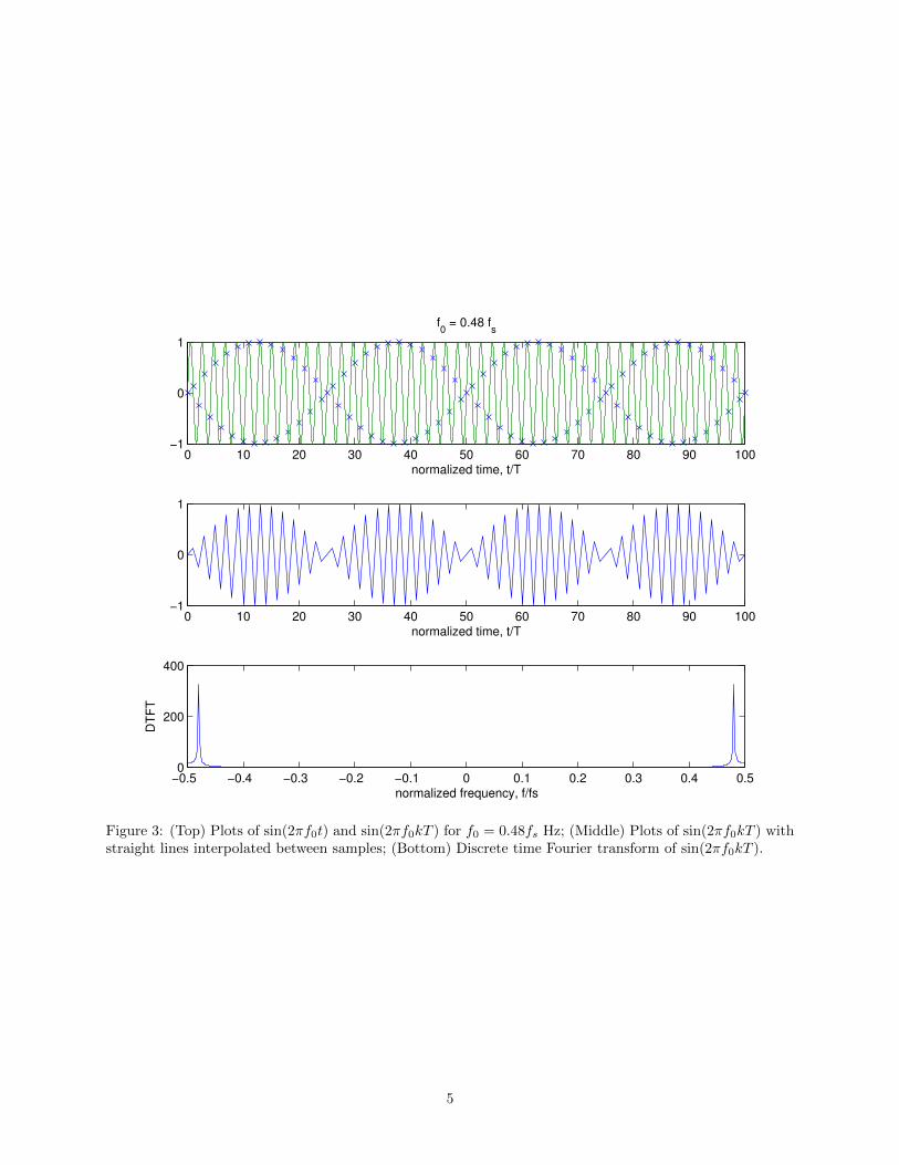
2.3 Signal Frequency Close to the Nyquist Frequency

Suppose that the signal frequency satisfies f0 ∈ ΩN , but is close to the Nyquist frequency. Then one mayexpect considerable distortion when comparing the sampled and analog signals. In fact, as we shall see inExample 3, the signal may appear to have a low frequency component. Before we present the example, let’ssee the reasons for this.

To study signals whose frequency lies close to the Nyquist frequency, it is convenient to denote thefrequency difference by ∆ = fN −f0. Then applying the trigonometric identity2 sin(α−β) = sin(α) cos(β)−cos(α) sin(β) yields

sin(2πf0kT ) = sin(2π(fN −∆)kT )

= sin(2πfNkT ) cos(2π∆kT )− cos(2πfNkT ) sin(2π∆kT ). (3)

Since fN = 1/2T , it follows that sin(2πfNkT ) = sin(πk) = 0, and thus

sin(2πf0kT ) = − cos(2πfNkT ) sin(2π∆kT ). (4)

We see that, after sampling, the signal looks like samples of a sine with frequency ∆ that are multiplied bysamples of a cosine with frequency fN . When ∆ is small, this produces a phenomenon similar to that ofbeats, familiar in the field of acoustics.

Finally, since cos(2πfNkT ) = cos(πk) = (−1)k, we have that

sin(2πf0kT ) = (−1)k+1 sin(2π∆kT ), (5)

and we see that the samples oscillate between positive and negative values.

Example 3 Suppose that f0 = 0.48fs Hz, only slightly below the Nyquist frequency fN = 0.5fs Hz. Then∆ = 0.02fs Hz, corresponding to a sine with period 1/∆ = 50T seconds. Figure 3 shows that the sampledsignal appears to have a 0.5fs Hz component (due to the oscillations between positive and negative values)that lies within an envelope of period 25T seconds (frequency 0.04fs Hz). The DTFT of the sampled signalshows that the sampled signal has only a 0.48fs Hz frequency component.

Each of the four segments of the middle plot in Figure 3 is referred to as a beat. Note that the beats areperiodic with period 25T seconds. Hence the beat frequency is given by fbeat = 2∆.

2http://en.wikipedia.org/wiki/List_of_trigonometric_identities#Angle_sum_and_difference_identities

4

0 10 20 30 40 50 60 70 80 90 100−1

0

1

normalized time, t/T

f0 = 0.48 f

s

0 10 20 30 40 50 60 70 80 90 100−1

0

1

normalized time, t/T

−0.5 −0.4 −0.3 −0.2 −0.1 0 0.1 0.2 0.3 0.4 0.50

200

400

normalized frequency, f/fs

DT

FT

Figure 3: (Top) Plots of sin(2πf0t) and sin(2πf0kT ) for f0 = 0.48fs Hz; (Middle) Plots of sin(2πf0kT ) withstraight lines interpolated between samples; (Bottom) Discrete time Fourier transform of sin(2πf0kT ).

5

2.4 Signal Frequency Close to the Half the Nyquist Frequency

You may also see a beat-like phenomenon when sampling a signal whose frequency is nearly half the Nyquistfrequency. Denote the difference between the frequency of the signal and half the Nyquist frequency by∆2 = fN/2− f0 Hz. Then

sin(2πf0kT ) = sin(2π(fN/2−∆2)kT )

= sin(2π(fN/2)kT ) cos(2π∆2kT )− cos(2π(fN/2)kT ) sin(2π∆2kT ), (6)

and we see that the sampled signal is the sum of two signals with frequency ∆2 Hz, each of whose amplitudeis multiplied by a signal with frequency fN/2 Hz. Since fN/2 = 1/2T , the coefficients sin(2π(fN/2)kT )and cos(2π(fN/2)kT ) alternate between 0 and ±1: for k = 0, 1, 2, 3, . . ., we have that sin(2π(fN/2)kT ) =0, 1, 0,−1, . . . and cos(2π(fN/2)kT ) = 1, 0,−1, 0, . . ..

Example 4 Suppose that f0 = 0.248fs Hz. Since fN/2 = 0.25fs Hz, it follows that ∆2 = 0.002fs Hz, orperiod 500T seconds. The top two plots in Figure 4 show that the sampled signal looks like overlappingversions of two signals that exhibit beats but are 90 out of phase. The DTFT shows that the signal hasfrequency 0.248fs Hz.

0 50 100 150 200 250 300 350 400 450 500−1

0

1

normalized time, t/T

f0 = 0.248 f

s

0 50 100 150 200 250 300 350 400 450 500−1

0

1

normalized time, t/T

−0.5 −0.4 −0.3 −0.2 −0.1 0 0.1 0.2 0.3 0.4 0.50

200

400

600

normalized frequency, f/fs

DT

FT

Figure 4: (Top) Plots of sin(2πf0t) and sin(2πf0kT ) for f0 = 0.252fs Hz; (Middle) Plots of sin(2πf0kT )with straight lines interpolated between samples; (Bottom) Discrete time Fourier transform of sin(2πf0kT ).

6

3 Why Do We See Beats?

We now explain why we sometimes see beats when we observe a signal on the virtual oscilloscope. To doso, we must first review the phenomenon of beats that is studied in the field of acoustics3, where it occurswith continuous time signals, and no sampling is involved. We then review the frequency spectrum of acontinuous time signal, and how that spectrum influences our ability to reconstruct the signal from only asubset of its samples, according to the Shannon sampling theorem. Finally, we show how use of an imperfectreconstruction scheme can result in the appearance of beats in the reconstructed signal.

3.1 Acoustic Beats

Beats occur when two analog time sine waves whose frequencies differ by only a small amount are addedor subtracted. To illustrate, consider two sine waves with different frequencies: sin(2πf1t) and sin(2πf2t).Using the trigonometric identity4 sinα± sinβ = 2 cos(0.5(α∓β)) sin(0.5(α±β)), the difference between thesine waves may be written as

1

2(sin(2πf1t)− sin(2πf2t)) = cos

(2π

(f1 + f2

2

)t

)sin

(2π

(f1 − f2

2

)t

)= − cos

(2π

(f1 + f2

2

)t

)sin

(2π

(f2 − f1

2

)t

). (7)

When f1 and f2 are approximately equal, the second term on the right of (7) is a low frequency sine wave,with frequency (f1 − f2)/2, that is multiplied by a cosine wave whose frequency is equal to the average ofthe two original sine wave frequencies, (f1 + f2)/2, and is thus much higher than the frequency of the sinewave. The frequency of the low frequency sine wave is equal to half the beat frequency, fbeat = f2 − f1.

Example 5 A plot of (7) for the values f1 = 0.48 Hz and f2 = 0.52 Hz is found in the top plot of Figure 5.With these values of f1 and f2, the beat frequency is fbeat = 0.04 Hz (period 25 seconds); the beat envelopesin (2π ((f2 − f1)/2) t) is found in the middle plot of Figure 5. The bottom plot of Figure 5 shows plotsof the individual sine waves sin(2πf1t) and − sin(2πf2t), together with their sum. Note how the size ofthe latter waxes and wanes corresponding to whether the individual sine waves are interfering more or lessconstructively or destructively.

The preceding analysis shows that adding two sine waves together may produce an interference patternthat appears to be a low frequency sine wave, even though a Fourier analysis of the resulting signal willreveal that only the frequencies of the two original sine waves are present.

To produce the phenomenon of beats, it is not necessary to work with the difference between the twosine waves on the left hand side of (7). Indeed, it is easy to verify that

1

2(sin(2πf1t) + sin(2πf2t)) = cos

(2π

(f1 − f2

2

)t

)sin

(2π

(f1 + f2

2

)t

). (8)

We see from (8) that the sum of two sine waves results in a low frequency cosine wave multiplied by a highfrequency cosine wave. We can also, of course obtain beats using cosine waves. For later reference, we notethat

1

2(cos(2πf1t) + cos(2πf2t)) = cos

(2π

(f1 + f2

2

)t

)cos

(2π

(f1 − f2

2

)t

), (9)

1

2(cos(2πf1t)− cos(2πf2t)) = − sin

(2π

(f1 + f2

2

)t

)sin

(2π

(f1 − f2

2

)t

). (10)

3http://en.wikipedia.org/wiki/Beat_(acoustics)4http://en.wikipedia.org/wiki/List_of_trigonometric_identities#Product-to-sum_and_sum-to-product_identities

7

0 10 20 30 40 50 60 70 80 90 100−1

0

1

f1 = 0.48 Hz, f

2 = 0.52 Hz, f

beat = 0.04 Hz

time, seconds

0 10 20 30 40 50 60 70 80 90 100−1

0

1

time, seconds

0 5 10 15 20 25−1

0

1

time, seconds

0.5sin(2πf1t)

−0.5sin(2πf2t)

0.5(sin(2πf1t)−sin(2πf

2t))

Figure 5: (Top) Plot of 0.5(sin(2πf1t)− sin(2πf2t)) for f1 = 0.48 Hz and f2 = 0.52 Hz, yielding beat period25 seconds; (Middle) The beat envelope sin(2π(fbeat/2)t); (Bottom) Plots of the sine waves 0.5 sin(2πf1t)and −0.5 sin(2πf2t), together with their sum.

8

3.2 Background Theory

Suppose that f(t) is an analog signal (not necessarily a sine function) with Fourier transform F (ω) = Ff(t)defined by

F (ω) =

∫ ∞−∞

f(t)e−jωtdt. (11)

For later reference, the time function f(t) can be recovered from its transform using the inverse Fouriertransform f(t) = F−1F (ω) defined by

f(t) =1

2π

∫ ∞−∞

F (ω)ejωtdω. (12)

Let us sample the analog signal f(t) with sample period T seconds, corresponding to sampling frequencyωs = 2π/T radians/second (fs = 1/T Hz) and Nyquist frequency ωN = π/T radians/second (fN = 1/2THz). Doing so results in a sequence of samples f(kT ), k = . . . ,−1, 0, 1, . . ..

The Shannon Sampling Theorem

The Shannon sampling theorem states conditions under which the time function f(t) may be completelyrecovered from its samples, implying that the sampling operation entails no loss of information. To bespecific, suppose that the spectrum of f(t) is bandlimited to frequencies below the Nyquist frequency; i.e.,suppose that

F (ω) = 0, |ω| ≥ ωN . (13)

Then in principle f(t) may be perfectly reconstructed from its samples using the formula

f(t) =

∞∑k=−∞

f(kT ) sinc

(t− kTT

), (14)

where sinc(x) , sin(πx)/πx. A plot of sinc(t/T ) vs t/T is shown in Figure 6.5

−5 −4 −3 −2 −1 0 1 2 3 4 5−0.4

−0.2

0

0.2

0.4

0.6

0.8

1

normalized time, t/T

Figure 6: A plot of sinc(t/T ) = sin(πt/T )/(πt/T ) vs t/T .

5Figure 6 is plotted with Matlab file sinc plot.m.

9

Approximate Reconstruction

We see from (14) that perfect reconstruction at time t requires all samples of the signal, both past andfuture, and hence cannot be implemented in real time. Instead, practical D/A converters approximate theanalog signal using finitely many samples. For example, one may use a staircase, or zero order hold (ZOH)approximation6, defined by

fZOH(t) , f(kT ), kT ≤ t < (k + 1)T. (15)

The virtual oscilloscope used in Lab 3 uses a trapezoidal, or first order hold (FOH) approximation7,

fFOH(t) , f(kT )

((k + 1)T − t

T

)+ f((k + 1)T )

(t− kTT

), kT ≤ t < (k + 1)T, (16)

that simply interpolates a straight line between successive sample points. Note that, unlike (15), the ap-proximation (16) cannot be computed in real time, because the approximation at time t ∈ (kT, (k + 1)T )depends upon the future sample to be taken sample at time (k + 1)T .

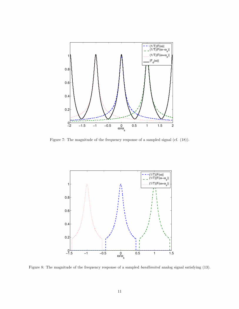
The Frequency Spectrum of a Sampled Signal

To understand what happens when the conditions of the sampling theorem are satisfied, but perfect recon-struction is not available, it is necessary to consider the frequency spectrum of a sampled signal. The discretetime Fourier transform (DTFT) of such a signal is defined as

Fd(ω) =

∞∑k=−∞

f(kT )e−jωkT . (17)

It is easy to see from (17) that the DTFT is periodic with period ωs: if ` is an integer, then Fd(ω + `ωs) =Fd(ω). Furthermore, the Poisson summation formula8 states that the frequency spectrum of a sampledsignal is equal to (1/T ) times the sum of infinitely many copies of the frequency spectrum (11) of theoriginal analog signal, with each copy shifted by an integer multiple of the sampling frequency:

Fd(ω) =1

T

∞∑k=−∞

F (ω − kωs). (18)

Example 6 The formula (18) is illustrated in Figure 7, for the time function f(t) = 0.5e−0.5t1(t), where1(t) denotes the unit step function.9 The resulting frequency response is F (ω) = 0.5/(jω + 0.5). Note thatthe spectrum of the sampled signal is periodic with period ωs, and that there is overlap between the variousshifted copies of the analog frequency spectrum.

Consider a hypothetical analog signal (11) whose frequency spectrum is bandlimited as in (13). Thenthe resulting discrete frequency spectrum may have the form illustrated in Figure 8. Note that there is nolonger any overlap between the shifted copies of the analog frequency response.

A Proof of the Shannon Sampling Theorem

The expression (18) for the frequency spectrum of a sampled signal may be used to obtain a proof of theShannon sampling theorem. The proof is instructive as it yields insight into the difference between ideal andapproximate reconstruction. Before providing the proof, we first provide a rigorous statement of the result.

6http://en.wikipedia.org/wiki/Zero-order_hold7http://en.wikipedia.org/wiki/First-order_hold8J. Braslavsky, G. Meinsma, R. Middleton, and J. Freudenberg, “On a key sampling formula relating the Laplace and z

transforms”, Systems & Control Letters, 29 (1997), pp. 181-190.9Figures 7-11 are plotted with Matlab file Poisson.m.

10

−2 −1.5 −1 −0.5 0 0.5 1 1.5 20

0.2

0.4

0.6

0.8

1

ω/ωs

(1/T)|F(ω)|(1/T)|F(ω−ω

s)|

(1/T)|F(ω+ωs)|

|Fd(ω)|

Figure 7: The magnitude of the frequency response of a sampled signal (cf. (18)).

−1.5 −1 −0.5 0 0.5 1 1.50

0.2

0.4

0.6

0.8

1

ω/ωs

(1/T)|F(ω)|(1/T)|F(ω−ω

s)|

(1/T)|F(ω+ωs)|

Figure 8: The magnitude of the frequency response of a sampled bandlimited analog signal satisfying (13).

11

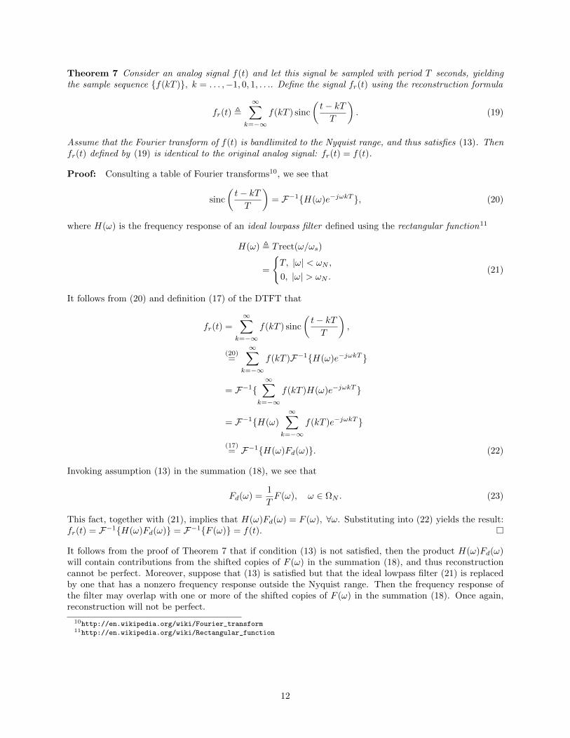
Theorem 7 Consider an analog signal f(t) and let this signal be sampled with period T seconds, yieldingthe sample sequence f(kT ), k = . . . ,−1, 0, 1, . . .. Define the signal fr(t) using the reconstruction formula

fr(t) ,∞∑

k=−∞

f(kT ) sinc

(t− kTT

). (19)

Assume that the Fourier transform of f(t) is bandlimited to the Nyquist range, and thus satisfies (13). Thenfr(t) defined by (19) is identical to the original analog signal: fr(t) = f(t).

Proof: Consulting a table of Fourier transforms10, we see that

sinc

(t− kTT

)= F−1H(ω)e−jωkT , (20)

where H(ω) is the frequency response of an ideal lowpass filter defined using the rectangular function11

H(ω) , T rect(ω/ωs)

=

T, |ω| < ωN ,

0, |ω| > ωN .(21)

It follows from (20) and definition (17) of the DTFT that

fr(t) =

∞∑k=−∞

f(kT ) sinc

(t− kTT

),

(20)=

∞∑k=−∞

f(kT )F−1H(ω)e−jωkT

= F−1∞∑

k=−∞

f(kT )H(ω)e−jωkT

= F−1H(ω)

∞∑k=−∞

f(kT )e−jωkT

(17)= F−1H(ω)Fd(ω). (22)

Invoking assumption (13) in the summation (18), we see that

Fd(ω) =1

TF (ω), ω ∈ ΩN . (23)

This fact, together with (21), implies that H(ω)Fd(ω) = F (ω), ∀ω. Substituting into (22) yields the result:fr(t) = F−1H(ω)Fd(ω) = F−1F (ω) = f(t).

It follows from the proof of Theorem 7 that if condition (13) is not satisfied, then the product H(ω)Fd(ω)will contain contributions from the shifted copies of F (ω) in the summation (18), and thus reconstructioncannot be perfect. Moreover, suppose that (13) is satisfied but that the ideal lowpass filter (21) is replacedby one that has a nonzero frequency response outside the Nyquist range. Then the frequency response ofthe filter may overlap with one or more of the shifted copies of F (ω) in the summation (18). Once again,reconstruction will not be perfect.

10http://en.wikipedia.org/wiki/Fourier_transform11http://en.wikipedia.org/wiki/Rectangular_function

12

Approximate Reconstruction: The Frequency Domain

We have seen that perfect reconstruction of a bandlimited signal according to the Shannon formula (14)requires the use of an ideal lowpass filter (21). It is instructive to compare the frequency response of such afilter to those of the approximate reconstruction schemes (15) and (16). These are given by

HZOH(ω) =1− e−jωT

jω, (24)

HFOH(ω) =ejωT

T

(1− e−jωT

jω

)2

. (25)

The magnitudes of the frequency responses (21), (24), and (25) are plotted in Figure 9. Note that both theZOH filter (24) and the FOH filter (25) have a nonzero frequency response outside the Nyquist range. Thisfact is significant because, as we have seen, the frequency spectrum of a sampled signal is periodic, and thusnonzero outside the Nyquist range even if the original analog signal satisfies (13).

−1.5 −1 −0.5 0 0.5 1 1.50

0.2

0.4

0.6

0.8

1

ω/ωs

(1/T)|H(ω)|(1/T)|H

ZOH(ω)|

(1/T)|HFOH

(ω)|

Figure 9: The frequency response of the ideal lowpass filter (21), the zero order hold (24), and the first orderhold (25), each normalized by (1/T ) to have unity height.

Application to a Sine Wave

Let us now see how the preceding ideas may be applied to the problem of approximately reconstructing asine wave. The Fourier transform of the f0 Hz sine wave, f(t) = sin(2πf0t) = sin(ω0t), is given by

F (ω) = jπ (δ(ω + ω0)− δ(ω − ω0)) , (26)

where ω0 = 2πf0 radians/second and δ(ω) is the delta function.12 For the remainder of this section, we workwith frequency in radians/second to simplify the formulas.

The Poisson summation formula (18) implies that the DTFT of the sampled sine wave f(kT ) = sin(ω0kT )satisfies

Fd(ω) =1

T

∞∑k=−∞

Fsin((ω0 − kωs)t). (27)

12To see why the Fourier transform of a sine wave with frequency ω0 has components at both ±ω0, recall that ejθ =(1/2)(cos θ+ j sin θ), from which it follows that sin θ = (1/2j)(ejθ− e−jθ). This identity, together with the fact that Fejωt =δ(ω − ω0), yields (26).

13

It is convenient to rewrite (27) as a sum of sinusoids whose frequencies will be nonnegative provided that0 ≤ ω0 < ωs. To do so, we note that

1

T

0∑k=−∞

Fsin((ω0 − kωs)t) =1

T

∞∑`=0

Fsin((ω0 + `ωs)t), (28)

1

T

∞∑k=1

Fsin((ω0 − kωs)t) =−1

T

∞∑k=1

Fsin((−ω0 + kωs)t). (29)

Substituting the identities (28)-(29) into (27) yields

Fd(ω) =1

T

∞∑`=0

Fsin((ω0 + `ωs)t) −1

T

∞∑k=1

Fsin((−ω0 + kωs)t), (30)

and we see that the frequency spectrum of the sampled sine wave is the weighted sum of the frequencyspectra of sine waves with frequencies ω0, ω0 + `ωs, ` = 1, . . .∞, and kωs − ω0, k = 1, . . .∞. A partial plotof the frequency spectrum given by (30) is shown in Figure 10 for a sine wave with ω0/ωs = 0.1; note weonly plot the terms in (30) corresponding to ` = 0, 1 and k = 1, 2.

-2 -1.5 -1 -0.5 0 0.5 1 1.5 2

ω/ωs

0

0.5

1

1.5

2

2.5

3

3.5

ω0/ω

s

1-ω0/ω

s

1+ω0/ω

s

2-ω0/ω

s

Figure 10: The normalized frequency spectrum of a sampled sine wave with frequency ω0/ωs = 0.1 showingthe terms due to ω0/ωs = 0.1, (ωs − ω0)/ωs = 0.9, (ωs + ω0)/ωs = 1.1, and (2ωs − ω0)/ωs = 1.9.

In the example illustrated in Figure 10, the signal frequency lies well below the Nyquist frequency. Ournext example illustrates what happens when this condition is not satisfied. Before proceeding, let us recalla fundamental property of linear time-invariant systems: the response of such a system to a sinusoid withspecified frequency is a sinusoid of the same frequency whose magnitude and phase are modified by the gainand phase of the system transfer function evaluated at the frequency of the input sinusoid. Furthermore,the superposition property of linear systems implies that the response to a sum of sinusoids is the sum ofthe responses to the individual sinusoids.

In our case, we are interested in the response of the reconstruction filters (21), (24), and (25) to thesignal sin(ωkT ), which has frequency spectrum Fd(ω) given by (30). The inverse Fourier transform of (30)is given by the time function fd(t) , F−1Fd(ω), where

fd(t) =1

T

∞∑`=0

sin((ω0 + `ωs)t)−1

T

∞∑k=1

sin((−ω0 + kωs)t). (31)

14

Note that all the sinusoids in (31) have positive frequencies, and that only one of them (` = 0) has a frequencylying below the Nyquist frequency.

Example 8 Let us return to Example 3, in which we saw the phenomenon of beats. In that example,f0 = 0.48 Hz and fN = 0.5 Hz, so that the signal frequency lies just below the Nyquist frequency. Accordingto (30), the DTFT of the sampled signal will have a term for ` = 0 that corresponds to sin(2π(0.48)t anda term for k = 1 that corresponds to sin(2π(0.52)t). The former results in Fd(ω) having delta functions at±0.48 and the latter to delta functions at ±0.52, as shown in Figure 11.

−2 −1.5 −1 −0.5 0 0.5 1 1.5 20

0.5

1

1.5

2

2.5

3

3.5

ω/ωs

|(1/T)H(ω)||(1/T)H

ZOH(ω)|

|(1/T)HFOH

(ω)|

|TFd(ω)|

Figure 11: The DTFT of sin(2π(0.48)t) together with the frequency responses of the ideal lowpass filter (21),the ZOH (24), and the FOH (25).

Let us now consider the result of reconstructing the original signal f(t) = sin(2πf0t) using three differentlowpass filters: H(ω) given by (21), HZOH(ω) given by (24), and HFOH(ω) given by (25). Denote the threereconstructed signals by fr(t), fZOH

r (t), and fFOHr (t), respectively.

First, since the summation (31) has only one term lying within below the Nyquist frequency, and sincethe frequency response of the ideal lowpass filter (21) is zero above the Nyquist frequency, reconstructionwith this filter will be perfect: fr(t) = f(t). (This also follows directly from Theorem 7.)

The other two reconstruction filters each have a frequency response that is nonzero above the Nyquistfrequency. As a result, the response of one of these filters to the signal (31) will have infinitely manycomponents. To illustrate, output of the first order hold in response to (31) is given by

fFOHr (t) =

1

T

∞∑`=0

|HFOH(ω0 + `ωs)| sin ((ω0 + `ωs)t− ∠(HFOH(ω0 + `ωs))

− 1

T

∞∑k=1

|HFOH(−ω0 + kωs)| sin((−ω0 + kωs)t− ∠(HFOH(−ω0 + kωs)). (32)

The term corresponding to ` = 0 in (32) is a sinusoid of frequency ω0,

fFOH`=0 (t) =

1

T|HFOH(ω0)| sin (ω0t− ∠(HFOH(ω0))) , (33)

and the term corresponding to k = 1 is a sinusoid of frequency (ωs − ω0)

fFOHk=1 (t) =

−1

T|HFOH((ωs − ω0))| sin ((ωs − ω0)t− ∠(HFOH(ωs − ω0))) . (34)

15

For our example, (33) and (34) have frequencies ω0 = 2π × 0.48 and ωs − ω0 = 2π × 0.52 radians/second,respectively. Hence, the sum of these two signals should yield a beat frequency of 2π×2(ωN −ω0) = 2π×0.4radians/second, as shown in Figure 12. By comparing Figure 12 with the middle plot in Figure 3, we seethat the reconstructed signal is reasonably well approximated by the sum of the first two sinusoids in (32);adding more terms in (32) would make the two plots identical.

0 10 20 30 40 50 60 70 80 90 100−1

−0.8

−0.6

−0.4

−0.2

0

0.2

0.4

0.6

0.8

1

time, seconds

f F OHℓ=0 (t ) + f F OH

k=1 (t )

Figure 12: The sum of sinusoids (33) and (34) approximates samples of sin(2π(0.48)t reconstructed using afirst order hold.

4 Summary

In this set of notes, we have considered distortion that may occur when reconstruction a signal from itssamples, even if the signal satisfies the hypotheses of the Shannon sampling theorem. The reason for thedistortion, which manifests itself as beats, is that the signal is not reconstructed using an ideal lowpassfilter. Use of a non-ideal filter, such as a zero order or first order hold, does not cause much distortion if thefrequency of the sampled signal is well below the Nyquist frequency. One the other hand, if the frequencyof the signal is just below the Nyquist frequency, then the observed distortion may be significant.

As usual in engineering, the perceptive question to ask is not “what happens when the hypotheses ofa theorem are satisfied”, but rather “what happens if the hypotheses are almost violated”. In the presentcase, we see that our sampling frequency should be significantly greater than the frequency content of oursampled signal, which is consistent with the recommendation in digital control textbooks that the samplingfrequency should be 10-20 times the bandwidth of the signal.

16