Sampling-Based Inference

1

Inference by stochastic simulation

Basic idea:1) Draw N samples from a sampling distribution S

Coin

0.52) Compute an approximate posterior probability P̂3) Show this converges to the true probability P

Outline:– Sampling from an empty network– Rejection sampling: reject samples disagreeing with evidence– Likelihood weighting: use evidence to weight samples– Markov chain Monte Carlo (MCMC): sample from a stochastic process

whose stationary distribution is the true posterior

2

Sampling from an empty network

function Prior-Sample(bn) returns an event sampled from bn

inputs: bn, a belief network specifying joint distribution P(X1, . . . , Xn)

x← an event with n elements

for i = 1 to n do

xi← a random sample from P(Xi | parents(Xi))

given the values of Parents(Xi) in x

return x

3

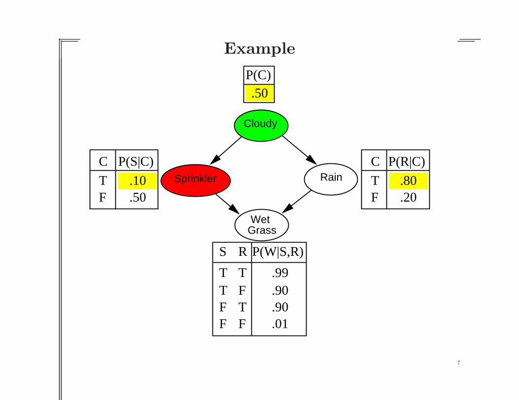
Example

Cloudy

RainSprinkler

WetGrass

C

TF

.80

.20

P(R|C)C

TF

.10

.50

P(S|C)

S R

T TT FF TF F

.90

.90

.99

P(W|S,R)

P(C).50

.01

4

Example

Cloudy

RainSprinkler

WetGrass

C

TF

.80

.20

P(R|C)C

TF

.10

.50

P(S|C)

S R

T TT FF TF F

.90

.90

.99

P(W|S,R)

P(C).50

.01

5

Example

Cloudy

RainSprinkler

WetGrass

C

TF

.80

.20

P(R|C)C

TF

.10

.50

P(S|C)

S R

T TT FF TF F

.90

.90

.99

P(W|S,R)

P(C).50

.01

6

Example

Cloudy

RainSprinkler

WetGrass

C

TF

.80

.20

P(R|C)C

TF

.10

.50

P(S|C)

S R

T TT FF TF F

.90

.90

.99

P(W|S,R)

P(C).50

.01

7

Example

Cloudy

RainSprinkler

WetGrass

C

TF

.80

.20

P(R|C)C

TF

.10

.50

P(S|C)

S R

T TT FF TF F

.90

.90

.99

P(W|S,R)

P(C).50

.01

8

Example

Cloudy

RainSprinkler

WetGrass

C

TF

.80

.20

P(R|C)C

TF

.10

.50

P(S|C)

S R

T TT FF TF F

.90

.90

.99

P(W|S,R)

P(C).50

.01

9

Example

Cloudy

RainSprinkler

WetGrass

C

TF

.80

.20

P(R|C)C

TF

.10

.50

P(S|C)

S R

T TT FF TF F

.90

.90

.99

P(W|S,R)

P(C).50

.01

10

Sampling from an empty network contd.

Probability that PriorSample generates a particular eventSPS(x1 . . . xn) = Πn

i = 1P (xi|parents(Xi)) = P (x1 . . . xn)i.e., the true prior probability

E.g., SPS(t, f, t, t) = 0.5× 0.9× 0.8× 0.9 = 0.324 = P (t, f, t, t)

Let NPS(x1 . . . xn) be the number of samples generated for event x1, . . . , xn

Then we have

limN→∞

P̂ (x1, . . . , xn) = limN→∞

NPS(x1, . . . , xn)/N

= SPS(x1, . . . , xn)

= P (x1 . . . xn)

That is, estimates derived from PriorSample are consistent

Shorthand: P̂ (x1, . . . , xn) ≈ P (x1 . . . xn)

11

Rejection sampling

P̂(X|e) estimated from samples agreeing with e

function Rejection-Sampling(X,e, bn,N) returns an estimate of P (X |e)

local variables: N, a vector of counts over X, initially zero

for j = 1 to N do

x←Prior-Sample(bn)

if x is consistent with e then

N[x]←N[x]+1 where x is the value of X in x

return Normalize(N[X])

E.g., estimate P(Rain|Sprinkler = true) using 100 samples27 samples have Sprinkler = true

Of these, 8 have Rain = true and 19 have Rain = false.

P̂(Rain|Sprinkler = true) = Normalize(〈8, 19〉) = 〈0.296, 0.704〉

Similar to a basic real-world empirical estimation procedure

12

Analysis of rejection sampling

P̂(X|e) = αNPS(X, e) (algorithm defn.)= NPS(X, e)/NPS(e) (normalized by NPS(e))≈ P(X, e)/P (e) (property of PriorSample)= P(X|e) (defn. of conditional probability)

Hence rejection sampling returns consistent posterior estimates

Problem: hopelessly expensive if P (e) is small

P (e) drops off exponentially with number of evidence variables!

13

Likelihood weighting

Idea: fix evidence variables, sample only nonevidence variables,and weight each sample by the likelihood it accords the evidence

function Likelihood-Weighting(X,e, bn,N) returns an estimate of P (X |e)

local variables: W, a vector of weighted counts over X, initially zero

for j = 1 to N do

x,w←Weighted-Sample(bn)

W[x ]←W[x ] + w where x is the value of X in x

return Normalize(W[X ])

function Weighted-Sample(bn,e) returns an event and a weight

x← an event with n elements; w← 1

for i = 1 to n do

if Xi has a value xi in e

then w←w × P (Xi = xi | parents(Xi))

else xi← a random sample from P(Xi | parents(Xi))

return x, w

14

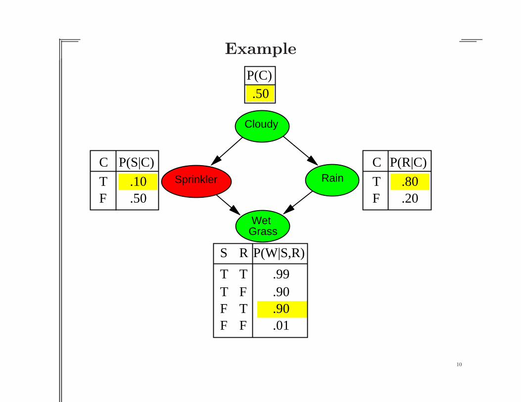
Likelihood weighting example

Cloudy

RainSprinkler

WetGrass

C

TF

.80

.20

P(R|C)C

TF

.10

.50

P(S|C)

S R

T TT FF TF F

.90

.90

.99

P(W|S,R)

P(C).50

.01

w = 1.0

15

Likelihood weighting example

Cloudy

RainSprinkler

WetGrass

C

TF

.80

.20

P(R|C)C

TF

.10

.50

P(S|C)

S R

T TT FF TF F

.90

.90

.99

P(W|S,R)

P(C).50

.01

w = 1.0

16

Likelihood weighting example

Cloudy

RainSprinkler

WetGrass

C

TF

.80

.20

P(R|C)C

TF

.10

.50

P(S|C)

S R

T TT FF TF F

.90

.90

.99

P(W|S,R)

P(C).50

.01

w = 1.0

17

Likelihood weighting example

Cloudy

RainSprinkler

WetGrass

C

TF

.80

.20

P(R|C)C

TF

.10

.50

P(S|C)

S R

T TT FF TF F

.90

.90

.99

P(W|S,R)

P(C).50

.01

w = 1.0× 0.1

18

Likelihood weighting example

Cloudy

RainSprinkler

WetGrass

C

TF

.80

.20

P(R|C)C

TF

.10

.50

P(S|C)

S R

T TT FF TF F

.90

.90

.99

P(W|S,R)

P(C).50

.01

w = 1.0× 0.1

19

Likelihood weighting example

Cloudy

RainSprinkler

WetGrass

C

TF

.80

.20

P(R|C)C

TF

.10

.50

P(S|C)

S R

T TT FF TF F

.90

.90

.99

P(W|S,R)

P(C).50

.01

w = 1.0× 0.1

20

Likelihood weighting example

Cloudy

RainSprinkler

WetGrass

C

TF

.80

.20

P(R|C)C

TF

.10

.50

P(S|C)

S R

T TT FF TF F

.90

.90

.99

P(W|S,R)

P(C).50

.01

w = 1.0× 0.1× 0.99 = 0.099

21

Likelihood weighting analysis

Sampling probability for WeightedSample is

SWS(z, e) = Πli = 1P (zi|parents(Zi))

Note: pays attention to evidence in ancestors onlyCloudy

RainSprinkler

WetGrass

⇒ somewhere “in between” prior andposterior distribution

Weight for a given sample z, e isw(z, e) = Πm

i = 1P (ei|parents(Ei))

Weighted sampling probability isSWS(z, e)w(z, e)

= Πli = 1P (zi|parents(Zi)) Πm

i = 1P (ei|parents(Ei))= P (z, e) (by standard global semantics of network)

Hence likelihood weighting returns consistent estimatesbut performance still degrades with many evidence variablesbecause a few samples have nearly all the total weight

22

Approximate inference using MCMC

“State” of network = current assignment to all variables.

Generate next state by sampling one variable given Markov blanketSample each variable in turn, keeping evidence fixed

function Gibbs-Sampling(X,e, bn,N) returns an estimate of P (X |e)

local variables: N[X ], a vector of counts over X, initially zero

Z, the nonevidence variables in bn

x, the current state of the network, initially copied from e

initialize x with random values for the variables in Y

for j = 1 to N do

for each Zi in Z do

sample the value of Zi in x from P(Zi |mb(Zi))

given the values of MB(Zi) in x

N[x ]←N[x ] + 1 where x is the value of X in x

return Normalize(N[X ])

Can also choose a variable to sample at random each time

23

The Markov chain

With Sprinkler = true, WetGrass = true, there are four states:

Cloudy

RainSprinkler

WetGrass

Cloudy

RainSprinkler

WetGrass

Cloudy

RainSprinkler

WetGrass

Cloudy

RainSprinkler

WetGrass

Wander about for a while, average what you see

24

MCMC example contd.

Estimate P(Rain|Sprinkler = true,WetGrass = true)

Sample Cloudy or Rain given its Markov blanket, repeat.Count number of times Rain is true and false in the samples.

E.g., visit 100 states31 have Rain = true, 69 have Rain = false

P̂(Rain|Sprinkler = true,WetGrass = true)= Normalize(〈31, 69〉) = 〈0.31, 0.69〉

Theorem: chain approaches stationary distribution:long-run fraction of time spent in each state is exactlyproportional to its posterior probability

25

Markov blanket sampling

Markov blanket of Cloudy isCloudy

RainSprinkler

WetGrass

Sprinkler and RainMarkov blanket of Rain is

Cloudy, Sprinkler, and WetGrass

Probability given the Markov blanket is calculated as follows:P (x′i|mb(Xi)) = P (x′i|parents(Xi))ΠZj∈Children(Xi)P (zj|parents(Zj))

Easily implemented in message-passing parallel systems, brains

Main computational problems:1) Difficult to tell if convergence has been achieved2) Can be wasteful if Markov blanket is large:

P (Xi|mb(Xi)) won’t change much (law of large numbers)

26

MCMC analysis: Outline

Transition probability q(x→ x′)

Occupancy probability πt(x) at time t

Equilibrium condition on πt defines stationary distribution π(x)Note: stationary distribution depends on choice of q(x→ x′)

Pairwise detailed balance on states guarantees equilibrium

Gibbs sampling transition probability:sample each variable given current values of all others

⇒ detailed balance with the true posterior

For Bayesian networks, Gibbs sampling reduces tosampling conditioned on each variable’s Markov blanket

27

Stationary distribution

πt(x) = probability in state x at time tπt+1(x

′) = probability in state x′ at time t + 1

πt+1 in terms of πt and q(x→ x′)

πt+1(x′) = Σxπt(x)q(x→ x′)

Stationary distribution: πt = πt+1 = π

π(x′) = Σxπ(x)q(x→ x′) for all x′

If π exists, it is unique (specific to q(x→ x′))

In equilibrium, expected “outflow” = expected “inflow”

28

Detailed balance

“Outflow” = “inflow” for each pair of states:

π(x)q(x→ x′) = π(x′)q(x′→ x) for all x, x′

Detailed balance ⇒ stationarity:

Σxπ(x)q(x→ x′) = Σxπ(x′)q(x′ → x)

= π(x′)Σxq(x′ → x)

= π(x′)

MCMC algorithms typically constructed by designing a transitionprobability q that is in detailed balance with desired π

29

Gibbs sampling

Sample each variable in turn, given all other variables

Sampling Xi, let X̄i be all other nonevidence variablesCurrent values are xi and x̄i; e is fixedTransition probability is given by

q(x→ x′) = q(xi, x̄i → x′i, x̄i) = P (x′i|x̄i, e)

This gives detailed balance with true posterior P (x|e):

π(x)q(x→ x′) = P (x|e)P (x′i|x̄i, e) = P (xi, x̄i|e)P (x′i|x̄i, e)

= P (xi|x̄i, e)P (x̄i|e)P (x′i|x̄i, e) (chain rule)

= P (xi|x̄i, e)P (x′i, x̄i|e) (chain rule backwards)

= q(x′ → x)π(x′) = π(x′)q(x′ → x)

30

Performance of approximation algorithms

Absolute approximation: |P (X|e)− P̂ (X|e)| ≤ ǫ

Relative approximation: |P (X|e)−P̂ (X|e)|P (X|e)

≤ ǫ

Relative ⇒ absolute since 0 ≤ P ≤ 1 (may be O(2−n))

Randomized algorithms may fail with probability at most δ

Polytime approximation: poly(n, ǫ−1, log δ−1)

Theorem (Dagum and Luby, 1993): both absolute and relativeapproximation for either deterministic or randomized algorithmsare NP-hard for any ǫ, δ < 0.5

(Absolute approximation polytime with no evidence—Chernoff bounds)

31