Sampling and Chapter Aliasing - UCCS College of ...mwickert/ece2610/lecture_notes/ece2610...Sampling...
24
ECE 2610 Signal and Systems 4–1 Sampling and Aliasing With this chapter we move the focus from signal modeling and analysis, to converting signals back and forth between the analog (continuous-time) and digital (discrete-time) domains. Back in Chapter 2 the systems blocks C-to-D and D-to-C were intro- duced for this purpose. The question is, how must we choose the sampling rate in the C-to-D and D-to-C boxes so that the analog signal can be reconstructed from its samples. The lowpass sampling theorem states that we must sample at a rate, , at least twice that of the highest frequency of interest in analog signal . Specifically, for having spectral con- tent extending up to B Hz, we choose in form- ing the sequence of samples . (4.1) Sampling • We have spent considerable time thus far, with the continu- ous-time sinusoidal signal , (4.2) where t is a continuous variable • To manipulate such signals in MATLAB or any other com- puter too, we must actually deal with samples of f s xt xt f s 1 T s 2 B = xn x nT s = – n xt A t + cos = xt Chapter 4
Transcript of Sampling and Chapter Aliasing - UCCS College of ...mwickert/ece2610/lecture_notes/ece2610...Sampling...

er
Sampling and AliasingWith this chapter we move the focus from signal modeling andanalysis, to converting signals back and forth between the analog(continuous-time) and digital (discrete-time) domains. Back inChapter 2 the systems blocks C-to-D and D-to-C were intro-duced for this purpose. The question is, how must we choose thesampling rate in the C-to-D and D-to-C boxes so that the analogsignal can be reconstructed from its samples.The lowpass sampling theorem states that we must sampleat a rate, , at least twice that of the highest frequency of interestin analog signal . Specifically, for having spectral con-tent extending up to B Hz, we choose in form-ing the sequence of samples
. (4.1)
Sampling
• We have spent considerable time thus far, with the continu-ous-time sinusoidal signal
, (4.2)
where t is a continuous variable
• To manipulate such signals in MATLAB or any other com-puter too, we must actually deal with samples of
fsx t x t
fs 1 Ts 2B=
x n x nTs = – n
x t A t + cos=
x t
Chapt
4
ECE 2610 Signal and Systems 4–1

Sampling
• Recall from the course introduction, that a discrete-time sig-nal can be obtained by uniformly sampling a continuous-timesignal at , i.e.,
– The values are samples of
– The time interval between samples is
– The sampling rate is
– Note, we could write
• A system which performs the sampling operation is called acontinuous-to-discrete (C-to-D) converter
tn nTs= x n x nTs =
x n x t
Tsfs 1 Ts=
x n x n fs =
IdealC-to-D
Converter
Ts
x t x n x nTs =
TsSimple SamplerSwitch Model
Analogto
DigitalConverter
ElectronicSubsystem:ADC or
SAR
x t x n x nTs =
x t x n x nTs =
Flash
Others
SAR = successive approximation register = delta-sigma modulator (oversampling)
A-to-D
B-bits, e.g., 16, 18
Momentarily close to take a sample
ECE 2610 Signals and Systems 4–2

Sampling
• A real C-to-D has imperfections, with careful design they canbe minimized, or at least have negligible impact on overallsystem performance
• For testing and simulation only environments we can easilygenerate discrete-time signals on the computer, with no needto actually capture and C-to-D process a live analog signal
• In this course we depict discrete-time signals as a sequence,and plot the corresponding waveform using MATLAB’s stemfunction, sometimes referred to as a lollypop plot>> n = 0:20;>> x = 0.8.^n;>> stem(n,x,'filled','b','LineWidth',2)>> grid>> xlabel('Time Index (n)')>> ylabel('x[n]')
0 2 4 6 8 10 12 14 16 18 200
0.1
0.2
0.3
0.4
0.5
0.6
0.7
0.8
0.9
1
Time Index (n)
x[n]
x n 0, n 0
0.8n, n 0
=
Waveform values only atinteger sample values
ECE 2610 Signals and Systems 4–3

Sampling
Sampling Sinusoidal Signals
• We will continue to find sinusoidal signals to be useful whenoperating in the discrete-time domain
• When we sample (4.2) we obtain a sinusoidal sequence
(4.3)
• Notice that we have defined a new frequency variable
rad, (4.4)
known as the discrete-time frequency or normalized continu-ous-time frequency
– Note that has units of radians, but could also be calledradians/sample, to emphasize the fact that sampling isinvolved
– Note also that many values of map to the same valueby virtue of the fact that is a system parameter that isnot unique either
– Since , we could also define as the dis-crete-time frequency in cycles/sample
Example: Sampling Rate Comparisons
• Consider at sampling rates of 240and 1000 samples per second
x n x nTs =
A nTs + cos=
A n + cos=
Ts fs----=
Ts
2f= f fTs
x t 2 60 t cos=
ECE 2610 Signals and Systems 4–4

Sampling
– The corresponding sample spacing values are
>> t = 0:1/2000:.02; >> x = cos(2*pi*60*t); % approx. to continuous-time>> t240 = 0:1/240:.02; >> n240 = 0:length(t240)-1;>> x240 = cos(2*pi*60/240*n240); % fs = 240 Hz>> axis([0 4.8 -1 1]) % axis scale since .02*240 = 4.8>> t1000 = 0:1/1000:.02;>> n1000 = 0:length(t1000)-1;>> x1000 = cos(2*pi*60/1000*n1000); % fs = 1000 Hz
Ts1
240--------- 4.1666 ms= = Ts
11000------------ 1ms= =
0 0.002 0.004 0.006 0.008 0.01 0.012 0.014 0.016 0.018 0.02−1
−0.5
0
0.5
1
Time (s)
x(t)
0 0.5 1 1.5 2 2.5 3 3.5 4 4.5−1
−0.5
0
0.5
1
x 240[n
]
0 2 4 6 8 10 12 14 16 18 20−1
−0.5
0
0.5
1
Sample Index (n)
x 1000
[n]
Continuous
fs = 240 Hz
fs = 1000 Hz
4 samples/period
16.67 samples/period
ECE 2610 Signals and Systems 4–5

Sampling
• The analog frequency is rad/s or 60 Hz
• When sampling with and 1000 Hz
respectively
• The sinusoidal sequences are
respectively
• It turns out that we can reconstruct the original fromeither sequence
• Are there other continuous-time sinusoids that when sam-pled, result in the same sequence values as and ?
• Are there other sinusoid sequences of different frequency that result in the same sequence values?
The Concept of Aliasing
• In this section we begin a discussion of the very importantsignal processing topic known as aliasing
• Alias as found in the Oxford American dictionary: noun
– A false or assumed identity: a spy operating under an alias.
– Computing: an alternative name or label that refers to a file, com-mand, address, or other item, and can be used to locate or access it.
2 60
fs 240=
240 2 60 240 2 0.25 rad= =
1000 2 60 1000 2 0.06 rad= =
x240 n 0.5n cos=
x1000 n 0.12n cos=
x t
x240 x1000
ECE 2610 Signals and Systems 4–6
Sampling
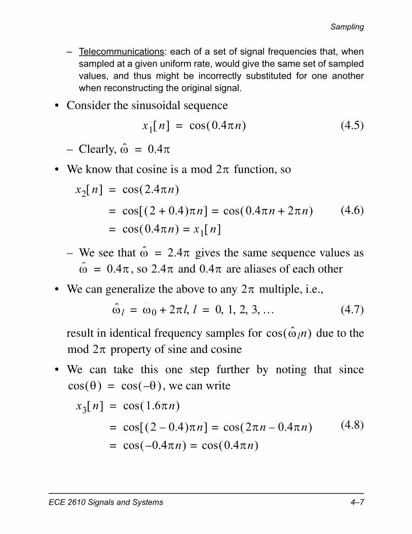
– Telecommunications: each of a set of signal frequencies that, whensampled at a given uniform rate, would give the same set of sampledvalues, and thus might be incorrectly substituted for one anotherwhen reconstructing the original signal.
• Consider the sinusoidal sequence
(4.5)
– Clearly,
• We know that cosine is a function, so
(4.6)
– We see that gives the same sequence values as, so and are aliases of each other
• We can generalize the above to any multiple, i.e.,
(4.7)
result in identical frequency samples for due to the property of sine and cosine
• We can take this one step further by noting that since, we can write
(4.8)
x1 n 0.4n cos=
0.4=
mod 2
x2 n 2.4n cos=
2 0.4+ n cos 0.4n 2n+ cos==
0.4n cos x1 n ==
2.4= 0.4= 2.4 0.4
2
l 0 2l+ l 0 1 2 3 = =
ln cosmod 2
cos – cos=
x3 n 1.6n cos=
2 0.4– n cos 2n 0.4n– cos==
0.4n– cos 0.4n cos==
ECE 2610 Signals and Systems 4–7

Sampling
– We see that gives the same sequence values as, so and are aliases of each other
• We can generalize this result to saying
(4.9)
result in identical frequency samples for due to the property and evenness property of cosine
– This result also holds for sine, expect the amplitude isinverted since
• In summary, for any integer l, and discrete-time frequency, the frequencies
(4.10)
all produce the same sequence values with cosine, and withsine may differ by the numeric sign
– A generalization to handle both cosine and sine is to con-sider the inclusion of an arbitrary phase ,
(4.11)
– Note in the second grouping the sign change in the phase
• The frequencies of (4.10) are aliases of each other, in termsof discrete-time frequencies
1.6= 0.4= 1.6 0.4
l 2l 0– l 0 1 2 3 = =
ln cosmod 2
– sin sin–=
0
0 0 2l+ 2l 0– l 1 2 3 =
A 2l+ n + cos A n 2l n + + cos=
A n + cos=
A 2l – n – cos A 2l n n– – cos=
A n– – cos=
A n + cos=
ECE 2610 Signals and Systems 4–8

Sampling
• The smallest value, , is called the principal alias
• These aliased frequencies extend to sampling a continuous-time sinusoid using the fact that or
, thus we may rewrite (4.10) in terms of the continu-ous-time frequency
(4.12)
– In terms of frequency in Hz we also have
(4.13)
• When viewed in the continuous-time domain, this means thatsampling with results in
(4.14)
being equivalent sequences for any n and any l
Example: Input a 60 Hz, 340 Hz, or 460 Hz Sinusoid with Hz
• The analog signal is
• We sample , i = 1, 2, 3 at rate Hz>> ta = 0:1/4000:2/60; % analog time axis>> xa1 = cos(2*pi*60*ta+pi/3);>> xa2 = cos(2*pi*340*ta-pi/3);
[0 )
Ts= Ts=fs=
0
0 0 2lfs+ 2lfs 0– l 1 2 3 =
f0 f0 lfs+ lfs f0– l 1 2 3 =
A 2f0t + cos t nTs
A 2f0 nTs + cos A 2 f0 lfs+ nTs + cos=
A 2 lfs f0– nTs – cos=
fs 400=
x1 t 260t 3+ cos=
x2 t 2340t 3– cos=
x3 t 2460t 3+ cos=
xi t fs 400=
ECE 2610 Signals and Systems 4–9

Sampling
>> xa3 = cos(2*pi*460*ta+pi/3);>> tn = 0:1/400:2/60; % discrete-time axis as n*Ts>> xn1 = cos(2*pi*60*tn+pi/3);>> xn2 = cos(2*pi*340*tn-pi/3);>> xn3 = cos(2*pi*460*tn+pi/3);
• We have used (4.14) to set this example up, so we expectedthe sample values for all three signals to be identical
• This shows that 60, 340, and 460, are aliased frequencies,when the sampling rate is 400 Hz
0 0.005 0.01 0.015 0.02 0.025 0.03 0.035−1
−0.5
0
0.5
1
x 1(t),
x1[n
]
0 0.005 0.01 0.015 0.02 0.025 0.03 0.035−1
−0.5
0
0.5
1
x 2(t),
x2[n
]
0 0.005 0.01 0.015 0.02 0.025 0.03 0.035−1
−0.5
0
0.5
1
Sample Index × Ts = nT
s (s)
x 3(t),
x3[n
]
f1 60 Hz = fs 400 Hz=
f2 340 Hz = fs 400 Hz=
f3 460 Hz = fs 400 Hz=
All the samplevalues match
AnalogDiscrete
ECE 2610 Signals and Systems 4–10

Sampling
– Note: 400 - 340 = 60 Hz and 460 - 400 = 60 Hz
• The discrete-time frequencies are
– Note: rad and rad
Example: versus
• To start with we need to see if either
for l a positive integer
• Solving the first equation, we see that , which is notan integer
• Solving the second equation, we see that , which is aninteger
• The phase does not agree with (4.11), so we will use MAT-LAB to see if tomake the samples agree in a time alignment sense
>> n = 0:10; % discrete time axis>> x1 = 5*cos(7.3*pi*n+pi/4);>> x2 = 5*cos(0.7*pi*n+pi/4);>> x3 = 5*cos(0.7*pi*n-pi/4);>> na = 0:1/200:10; % continuous time axis>> x1a = 5*cos(7.3*pi*na+pi/4);
i 0.3 1.7 2.3 =
2 1.7– 0.3= 2.3 2– 0.3=
5 7.3n 4+ cos 5 0.7n 4+ cos
7.3 0.7 2l+=
or 7.3 2l 0.7–=
l 3.3=
l 4=
0 2 3 4 5 6 7 8
0.7 7.3
What are some other valid alias frequencies?
5 0.7n 4+ cos 5 0.7n 4– cos
ECE 2610 Signals and Systems 4–11

Sampling
>> x2a = 5*cos(0.7*pi*na+pi/4);>> x3a = 5*cos(0.7*pi*na-pi/4);
The Spectrum of a Discrete-Time Signal
• As alluded to in the previous example, a spectrum plot can behelpful in understanding aliasing
• From the earlier discussion of line spectra, we know that foreach real cosine at , the result is spectral lines at
• When we consider the aliased frequency possibilities for asingle real cosine signal, we have spectral lines not only at
, but at all frequency offsets, that is
0 1 2 3 4 5 6 7 8 9 10−5
0
5
x 1[n]
0 1 2 3 4 5 6 7 8 9 10−5
0
5
x 2[n]
0 1 2 3 4 5 6 7 8 9 10−5
0
5
x 3[n]
Sample Index (n)
Agr
ee
Sam
ple
s m
atch
,bu
t wro
ng p
hase
5 7.3n 4+ cos
5 0.7n 4+ cos
5 0.7n 4– cos
0 0
0 2l
ECE 2610 Signals and Systems 4–12

Sampling
(4.15)
• The principal aliases occur when , as these are the onlyfrequencies on the interval
Example:
• The line spectra plot of this discrete-time sinusoid is shownbelow
• A particularly useful view of the alias frequencies is to con-sider a folded strip of paper, with folds at integer multiples of
, with the strip representing frequencies along the -axis
0 2l l 0 1 2 3 =
l 0=[ )–
x n 0.4n cos=
2 3–2–3– 0
. . .. . .
00–
PrincipalAliases1
2----2 Offset 2 Offset
0
2
3
4
–
Folded Strip is the Axis
0 2 0– 0 2+– 02– 0+ 4 0–
All of the alias frequencies are on a the same line when the paperis folded like an accordian, hence the term folded frequencies.
Principlealias range
ECE 2610 Signals and Systems 4–13
Sampling
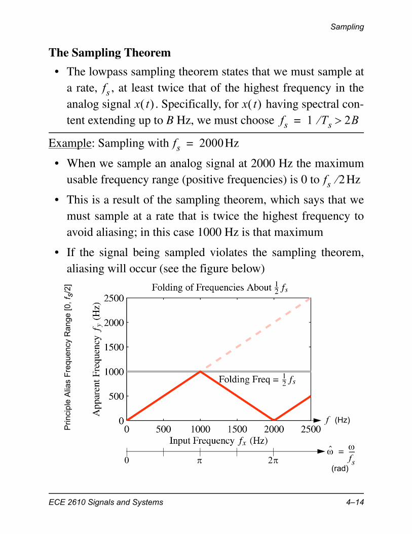
The Sampling Theorem
• The lowpass sampling theorem states that we must sample ata rate, , at least twice that of the highest frequency in theanalog signal . Specifically, for having spectral con-tent extending up to B Hz, we must choose
Example: Sampling with Hz
• When we sample an analog signal at 2000 Hz the maximumusable frequency range (positive frequencies) is 0 to Hz
• This is a result of the sampling theorem, which says that wemust sample at a rate that is twice the highest frequency toavoid aliasing; in this case 1000 Hz is that maximum
• If the signal being sampled violates the sampling theorem,aliasing will occur (see the figure below)
fsx t x t
fs 1 Ts 2B=
fs 2000=
fs 2
fs----=
0 2
f
(rad)
(Hz)
Prin
cipl
e A
lias
Fre
quen
cy R
ange
[0,
f s/2
]
ECE 2610 Signals and Systems 4–14
Sampling
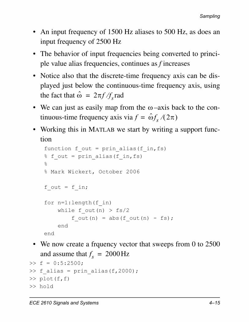
• An input frequency of 1500 Hz aliases to 500 Hz, as does aninput frequency of 2500 Hz
• The behavior of input frequencies being converted to princi-ple value alias frequencies, continues as f increases
• Notice also that the discrete-time frequency axis can be dis-played just below the continuous-time frequency axis, usingthe fact that rad
• We can just as easily map from the –axis back to the con-tinuous-time frequency axis via
• Working this in MATLAB we start by writing a support func-tion function f_out = prin_alias(f_in,fs)% f_out = prin_alias(f_in,fs)%% Mark Wickert, October 2006
f_out = f_in;
for n=1:length(f_in) while f_out(n) > fs/2 f_out(n) = abs(f_out(n) - fs); endend
• We now create a frquency vector that sweeps from 0 to 2500and assume that Hz
>> f = 0:5:2500;>> f_alias = prin_alias(f,2000);>> plot(f,f)>> hold
2f fs=
f fs 2 =
fs 2000=
ECE 2610 Signals and Systems 4–15

Sampling
Current plot held>> plot(f,f_alias,'r')>> grid>> xlabel('Frequency (Hz)')>> ylabel('Apparent Frequency (Hz)')>> print -tiff -depsc f_alias.eps
Example: Compact Disk Digital Audio
• Compact disk (CD) digital audio uses a sampling rate of kHz
• From the sampling theorem, this means that signals havingfrequency content up to 22.05 kHz can be represented
• High quality audio signal processing equipment generallyhas an upper frequency limit of 20 kHz
– Musical instruments can easily produce harmonics above20 kHz, but human’s cannot hear these signals
0 500 1000 1500 2000 25000
500
1000
1500
2000
2500
Frequency (Hz)
App
aren
t Fre
quen
cy (
Hz)
Before sampling
After samplingwith fs = 2000 Hz
fs 44.1=
ECE 2610 Signals and Systems 4–16

Sampling
• The fact that aliasing occurs when the sampling theorem isviolated leads us to the topic of reconstructing a signal fromits samples
• In the previous example with Hz, we see that tak-ing into account the principle alias frequency range, theusable frequency band is only [0, 1000] Hz
Ideal Reconstruction
• Reconstruction refers using just the samples to return to the original continuous-time signal
• Ideal reconstruction refers to exact reconstruction of from its samples so long as the sampling theorem is satisfied
• In the extreme case example, this means that a sinusoid hav-ing frequency just less than , can be reconstructed fromsamples taken at rate
• The block diagram of an ideal discrete-to-continuous (D-to-C) converter is shown below
• In very simple terms the D-to-C performs interpolation on thesample values as they are placed on the time axis atspacing s
fs 2000=
x n x nTs =x t
x t
fs 2fs
IdealD-to-C
Convertery n y t
fs1Ts-----=
y n Ts
ECE 2610 Signals and Systems 4–17
Sampling
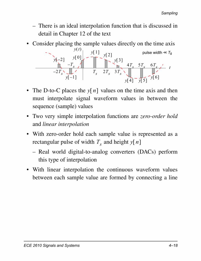
– There is an ideal interpolation function that is discussed indetail in Chapter 12 of the text
• Consider placing the sample values directly on the time axis
• The D-to-C places the values on the time axis and thenmust interpolate signal waveform values in between thesequence (sample) values
• Two very simple interpolation functions are zero-order holdand linear interpolation
• With zero-order hold each sample value is represented as arectangular pulse of width and height
– Real world digital-to-analog converters (DACs) performthis type of interpolation
• With linear interpolation the continuous waveform valuesbetween each sample value are formed by connecting a line
t
y t
y 0
y 1–
y 2–
y 1 y 2
y 3
y 4 y 5 y 6
Ts 2Ts 3Ts
4Ts 5Ts 6TsT– s2T– s
pulse width << Ts
y n
Ts y n
ECE 2610 Signals and Systems 4–18

Sampling
between the values
• Both cases introduce errors, so it is clear that something bet-ter must exist
• For D-to-C conversion using pulses, we can write
(4.16)
where is a rectangular pulse of duration
• A complete sampling and reconstruction system requiresboth a C-to-D and a D-to-C
y n
t
y t
y 0
y 1–
y 2– y 1 y 2 y 3
y 4 y 5 y 6
Ts 2Ts 3Ts
4Ts5Ts 6Ts
T– s
2T– s
t
y t
y 0
y 1–
y 2–
y 1 y 2
y 3
y 4 y 5 y 6
Ts 2Ts 3Ts
4Ts 5Ts 6TsT– s2T– s
Zero-OrderHold Interp.
LinearInterp.
Similar to actualDAC output
y t y n p t nTs– n –=
=
p t Ts
IdealD-to-C
Converter
IdealC-to-D
Converter
DirectConnection
DSP System
x t y t x n y n
y n x n =fs fs
ECE 2610 Signals and Systems 4–19
Sampling
• With this system we can sample analog signal to pro-duce , and at the very least we may pass directly to
, then reconstruct the samples into
– The DSP system that sits between the C-to-D and D-to-C,should do something useful, but as a starting point we con-sider how well a direct connection system does at returning
– As long as the sampling theorem is satisfied, we expectthat will be close to for frequency content in that is less than Hz
– What if some of the signals contained in do not satisfythe sampling theorem?
– Typically the C-to-D is designed to block signals above from entering the C-to-D (antialiasing filter)
– A practical D-to-C is designed to reconstruct the principlealias frequencies that span
(4.17)
x t x n x n
y n y n y t
y t x t
y t x t x t fs 2
x t
fs 2
– f fs 2 fs 2–
ECE 2610 Signals and Systems 4–20

Spectrum View of Sampling and Reconstruction
Spectrum View of Sampling and Reconstruc-tion
• We now view the spectra associated with a cosine signalpassing through a C-to-D/D-to-C system
• Assume that
• The sampling rate will be fixed at Hz
x t 2f0t cos=
fs 2000=
f
f
f
Spectrum of 500 Hz Cosine x(t)
2–2– 0
200010001000–2000– 0
200010001000–2000– 0
200010001000–2000– 0
Spectrum of Sampled 500 Hz Cosine x[n] = y[n]
Spectrum of Reconstructed 500 Hz Cosine y(t)
fs 2000 Hz=12---
12---
12--- Reconstruction
Band
500-500
0.5-0.5
500-500
AliasAliasAliasAlias
(Hz)
(Hz)
(Hz)
(rad)
ECE 2610 Signals and Systems 4–21

Spectrum View of Sampling and Reconstruction
• We see that the 1500 Hz sinusoid is aliased to 500 Hz, andwhen it is output as , we have no idea that it arrived at theinput as 1500 Hz
• What are some other inputs that will produce a 500 Hz out-put?
The Ideal Bandlimited Interpolation
• In Chapter 12 of the text it is shown that ideal D-to-C conver-sion utilizes an interpolating pulse shape of the form
(4.18)
f
f
f
Spectrum of 1500 Hz Cosine x(t)
2–2– 0
200010001000–2000– 0
200010001000–2000– 0
200010001000–2000– 0
Spectrum of Sampled 1500 Hz Cosine x[n] = y[n]
Spectrum of Reconstructed 1500 Hz Cosine y(t)
fs 2000 Hz=12---
12---
12---
500-500
1.5-1.5 0.5-0.5
500-500
AliasAliasAlias Alias
ReconstructionBand
(Hz)
(Hz)
(Hz)
(rad)
y t
p t t Ts sin
t Ts --------------------------- – t =
ECE 2610 Signals and Systems 4–22

Spectrum View of Sampling and Reconstruction
• The function is known as the sinc function
• Note that interpolation with this function means that all sam-ples are required to reconstruct , since the extent of is doubly infinite
– In practice this form of reconstruction is not possible
• A Mathematica animation showing that when the sinc()pulses are weighted by the sample values, delayed, and thensummed, high quality reconstruction (interpolation) is possi-ble
– The code used to create the animation
x sin x
y t p t
-7.5 -5 -2.5 2.5 5 7.5
-0.2
0.2
0.4
0.6
0.8
1p t
tTs-----
Zero crossingsat integer multiplesof Ts
Manipulate@Show@Plot@Cos@2 p f t + fD, 8t, 0, 10<, PlotStyle Ø [email protected], RGBColor@1, 0, 0D<D,Plot@Sum@Cos@2 p f n + fD Sinc@p Ht - nLD, 8n, 0, 10<D, 8t, 0, 10<,PlotStyle Ø 8Thick, RGBColor@0, 1, 0D<D, DiscretePlot@Cos@2 p f n + fD,8n, 0, 10<, Filling Ø Axis, PlotStyle Ø [email protected], RGBColor@1, 0, 0D<D,
Plot@Table@Cos@2 p f n + fD Sinc@p Ht - nLD, 8n, 0, 10<D, 8t, 0, 10<, PlotRange Ø AllD,PlotRange Ø AllD,
88f, 1 ê 10<, 81 ê 2, 1 ê 3, 1 ê 4, 1 ê 10, 1 ê 20<<, 88f, 0<, 80, p ê 4, p ê 2<<D
ECE 2610 Signals and Systems 4–23

Spectrum View of Sampling and Reconstruction
• The final display showing an interpolated output for a singlesinusoid
– The input signal is and we assumethat , so in sampling we let
– With (4 samples per period) and wehave the following display:
x t 2ft + cos=Ts 1= t n
f 1 4= 4=
f 12
13
14
110
120
f 0 p
4p
2
Green thick = intepolated outputRed dashed = inputBlue thin = sinc interpolated samplesRed points = sample value
ECE 2610 Signals and Systems 4–24